
Chris Parmer
November 15, 2026
Stacked Bar Charts - A Complete Guide
TL;DR
- A stacked bar chart splits each bar into segments, one per part, so the length of the bar shows the total and each segment shows one part of it. It works best when the total matters and only one or two of the parts do. The bar chart guide covers stacking briefly, and this guide goes deeper.
- Stacked bar charts are also known as composite bar charts and, when the bars are vertical, stacked column charts. Scaled to 100%, they are called 100% stacked or percent stacked bar charts. They are similar to grouped bar charts and stacked area charts.
- Only the first segment and the total sit on a common baseline, so only those are easy to compare between bars. Put the segment that matters most at the bottom, print the totals, and switch to a 100% stack when the mix matters more than the size or to grouped bars when the parts need comparing.
- When the parts have a positive and a negative side, such as exports and imports or agree and disagree, a diverging stack puts them on either side of zero (see the Likert chart guide for survey answers). Close relatives change the scale, the width or the mark, such as the 100% stack, the Marimekko chart (also called a mosaic chart), the dot plot, the waffle chart and the population pyramid, and a section below shows each on real data.
- You can make every version with Plotly in one line of code: px.bar in Python or barmode: "stack" in plotly.js. This guide has 11 examples on real data, from exoplanets and electricity to Federal Reserve assets and clinical trials.
What is a stacked bar chart?
Stacked bar charts look like this:
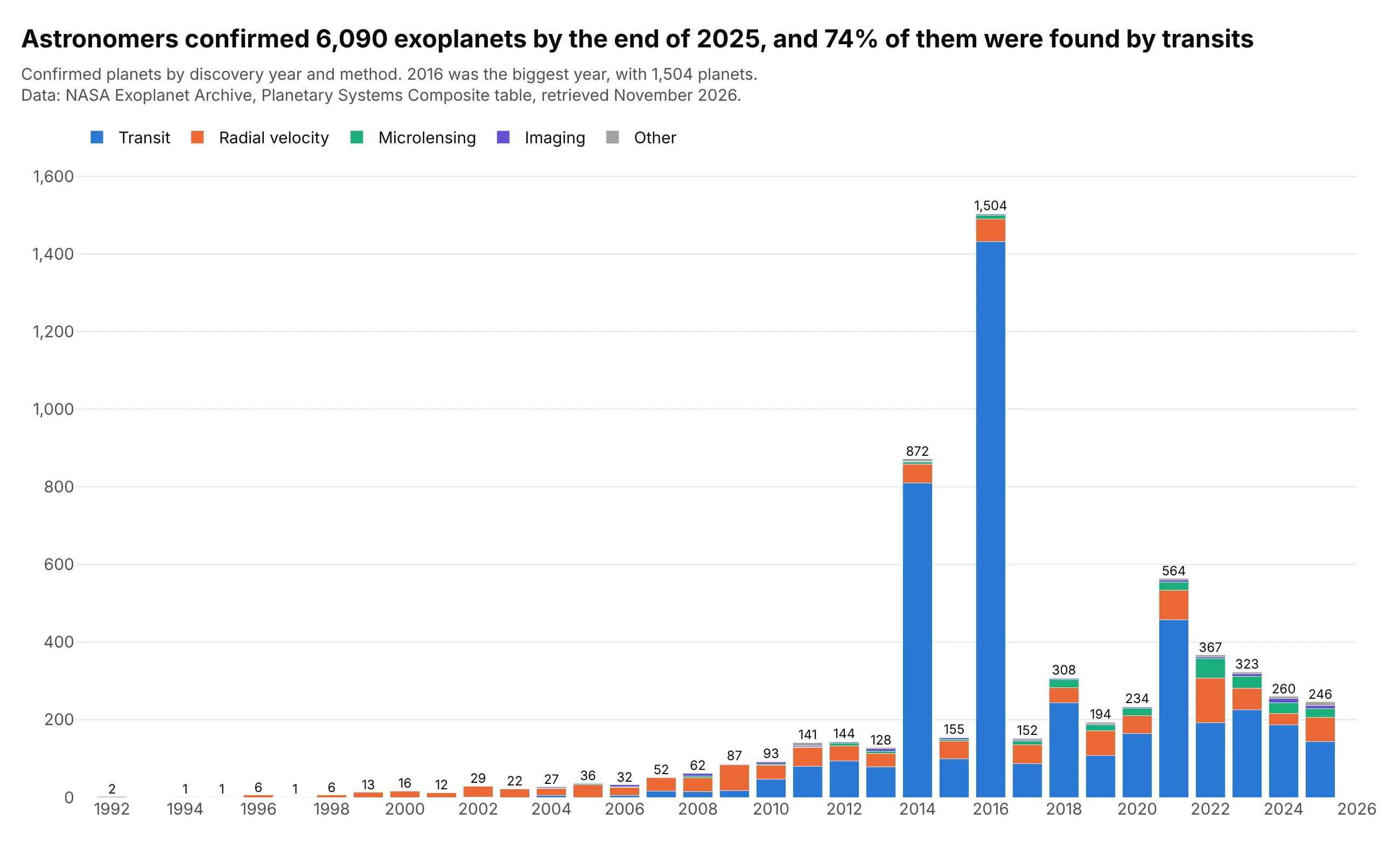
Data: NASA Exoplanet Archive, Planetary Systems Composite table, retrieved November 2026.
How do you read a stacked bar chart? In the example above, notice these things:
- Each column is one discovery year, and the whole column is every planet confirmed that year. Its total is printed on top, so you never have to add the segments up: 1,504 planets in 2016 against 564 in 2021.
- The blue segment at the bottom, planets found by watching a star dim as a planet crosses in front of it (the transit method), starts at zero in every column. Its heights can be compared directly, 1,432 in 2016 against 457 in 2021.
- Each segment above blue starts where the one below it ends, so the orange segment for the radial velocity method (a star's wobble as a planet pulls on it) starts at a different height every year. Comparing its size between years, 77 planets in 2021 and 115 in 2022, takes more effort than comparing the blue ones.
- Colors and order are fixed, with the biggest method at the bottom and the smallest at the top, so the same method is in the same place in every column. The small methods are grouped as "Other" because a segment of a handful of planets can't be read in a stack.
- The tall columns in 2014 and 2016 come from NASA announcements of 715 and 1,284 planets validated at once from the Kepler space telescope's data. 2026 is left out because the year isn't finished.
It's often used for charts like these:
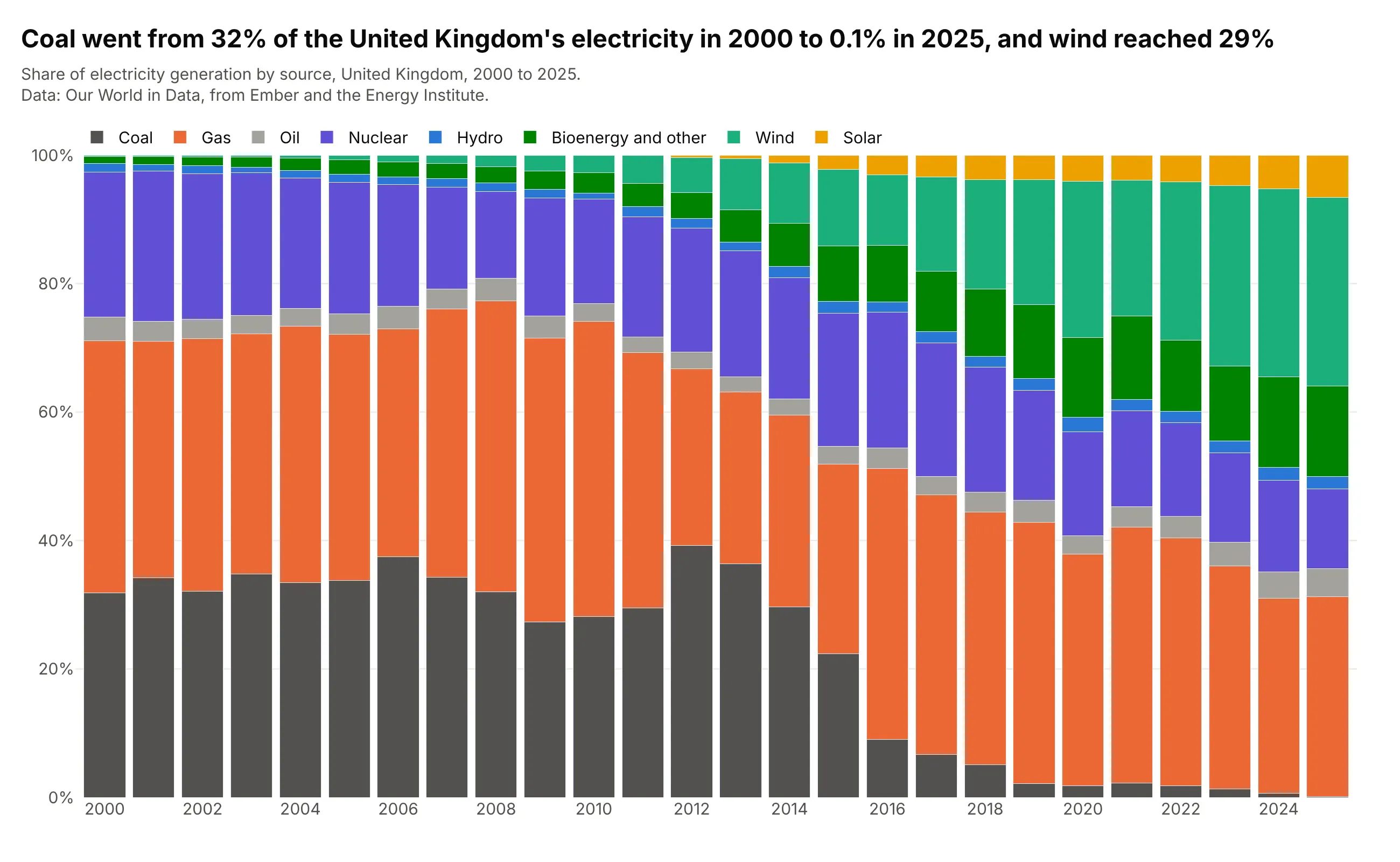
A mix that changes over time. Coal made 32% of the United Kingdom's electricity in 2000 and 0.1% in 2025, while wind went from 0.2% to 29%, and the 100% stack shows the whole mix moving at once. Data: Our World in Data, from Ember and the Energy Institute.
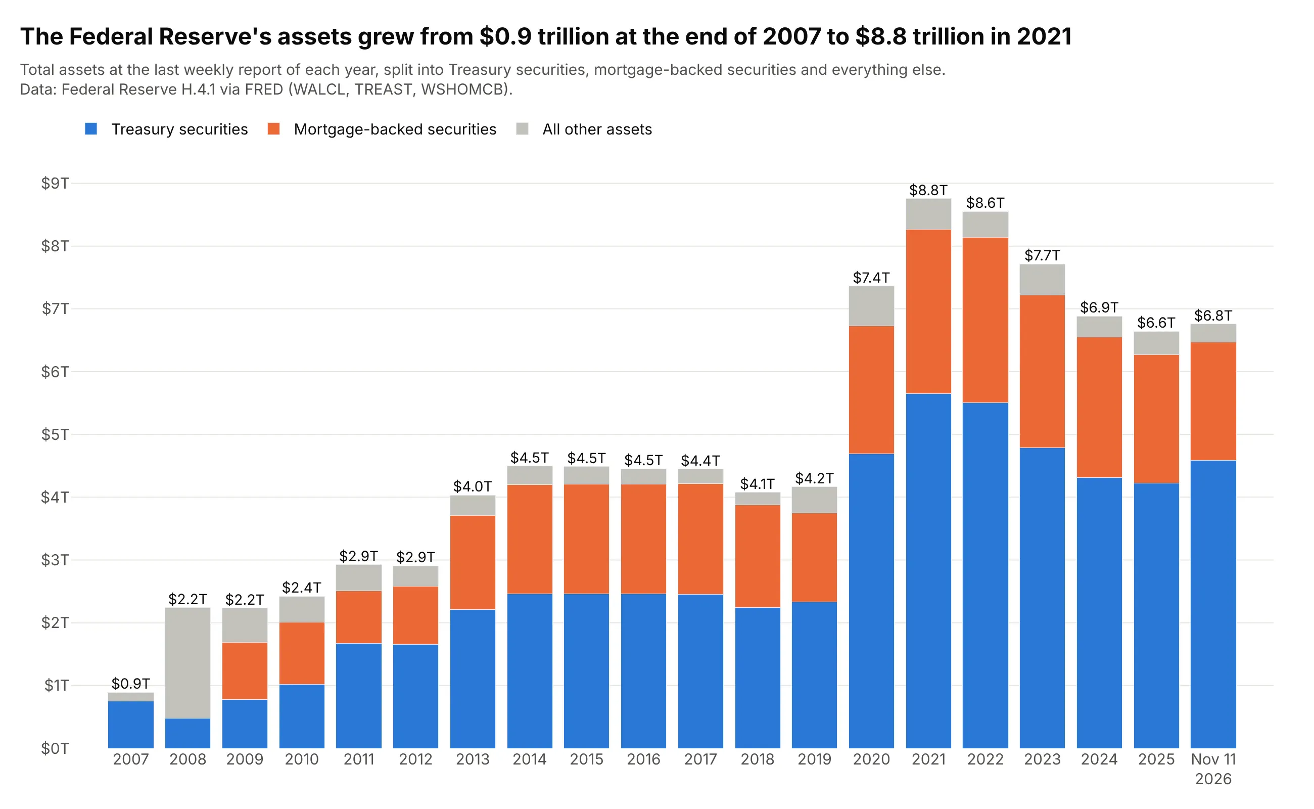
A total built from a few parts, in finance. The Federal Reserve's assets grew from $0.9 trillion at the end of 2007 to $8.8 trillion at the end of 2021, and the stack shows that the growth was mostly Treasury securities, then mortgage-backed securities. Data: Federal Reserve H.4.1 via FRED (Federal Reserve Economic Data).
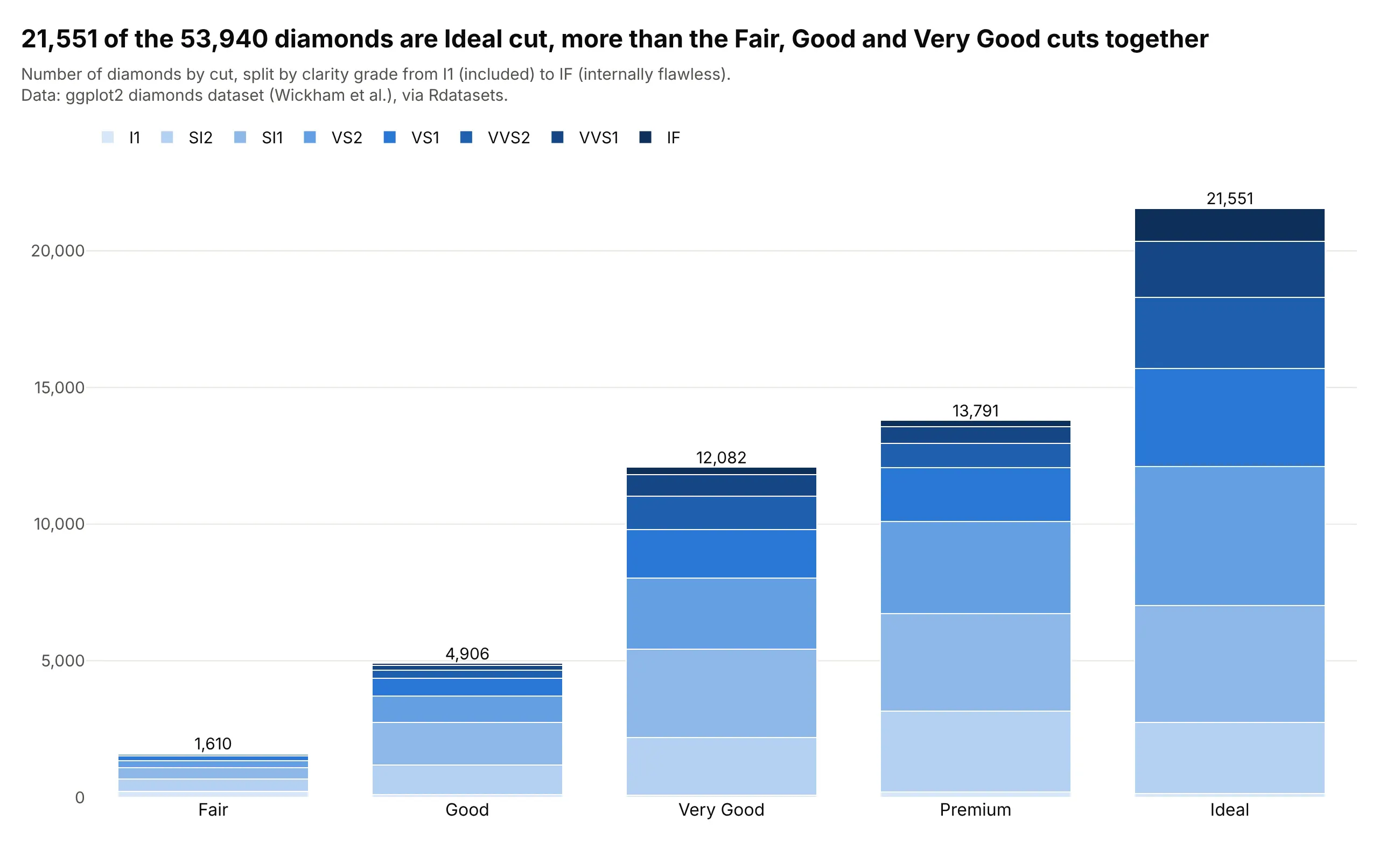
The textbook example. The diamonds dataset is the example R for Data Science uses to teach stacked bars in ggplot2 (geom_bar with fill = clarity): 21,551 of its 53,940 diamonds are Ideal cut, and each column splits into clarity grades. Data: ggplot2 diamonds dataset, via Rdatasets.
A short history
Many sources consider William Playfair the inventor of the bar chart. His Commercial and Political Atlas of 1786 has one bar chart, which draws a year of Scotland's trade as a pair of bars, imports and exports, for each of 17 trading partners (Wikipedia). Putting the two bars end to end gives the total trade with each place, which is the question a stacked bar answers:
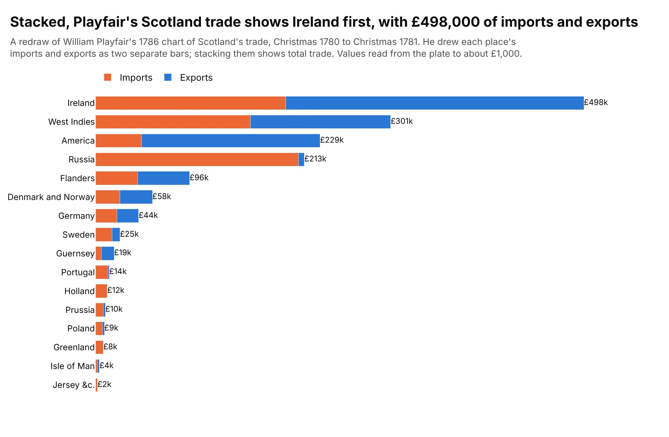
Data: values read from Playfair's plate in a public-domain scan on Wikimedia Commons, to about £1,000. Playfair drew the bars side by side, so this is his data stacked, not his chart.

Stacked bars are now built into spreadsheets and statistics software, where Excel calls them stacked columns and stacked bars. The weakness that the next section describes was measured in 1984 by Cleveland and McGill, who ranked position along a common scale as the most accurately judged way to read a value from a chart, ahead of position along scales that don't line up (1984). Naomi Robbins and Richard Heiberger later made the case for centering the stacks of rating scales on zero, in 2011 and then in full in the Journal of Statistical Software (2014), which is the diverging stack below.
When stacking works, and the baseline problem
A stacked bar answers two questions well, how big is the total and how big is the bottom segment, because both start at zero. Every other segment floats on top of the ones below it. Here are the same fuels drawn stacked and then alone:
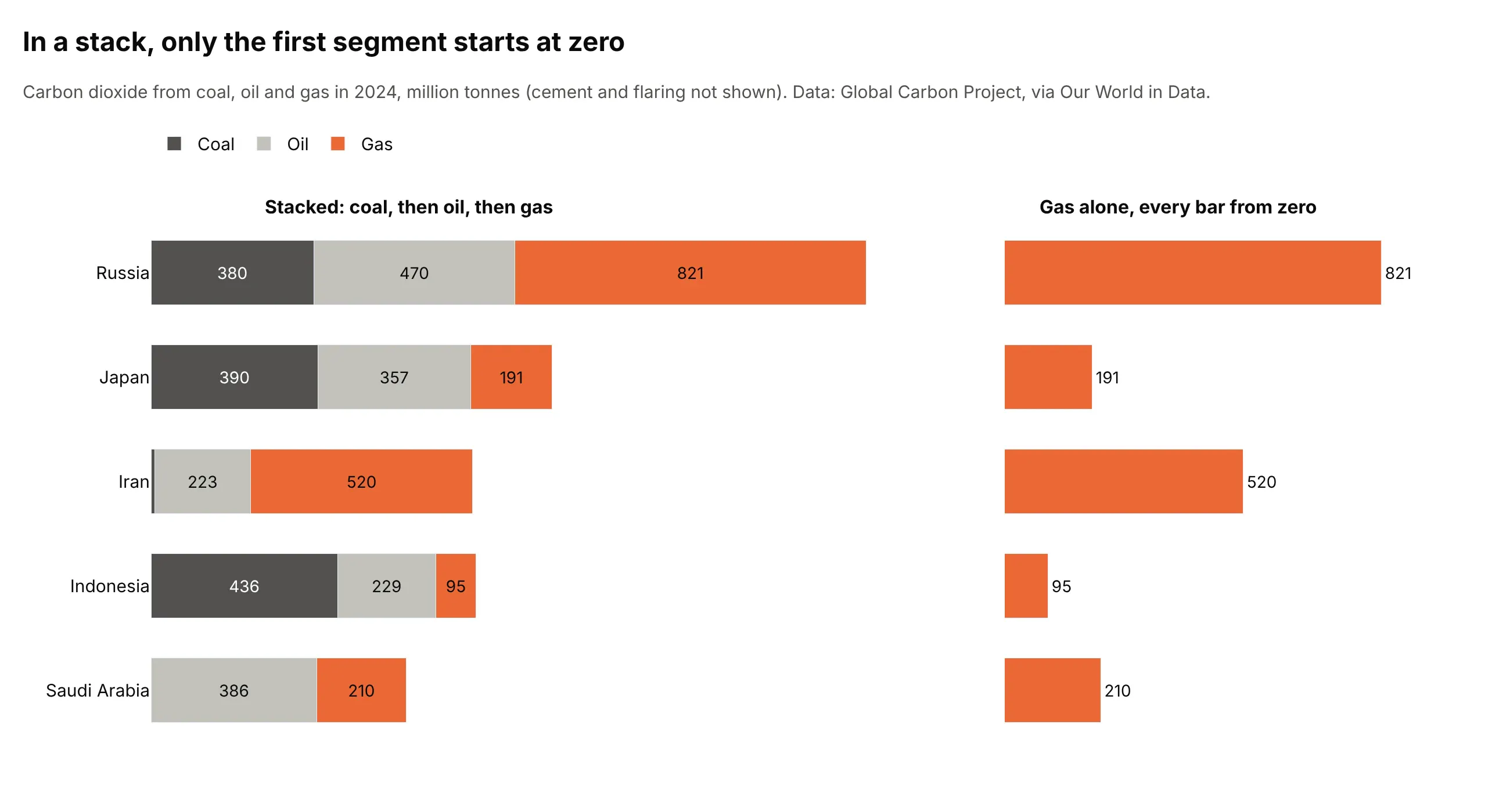
Data: Global Carbon Project, via Our World in Data. Cement and flaring are not shown.
In the stacked panel, gas is on top, so Russia's gas segment runs from 850 to 1,671 million tonnes and Iran's from 232 to 752. You can see that Russia's is longer only by comparing two lengths that start in different places, and you can't see how much longer without the printed values. In the right panel every gas bar starts at zero, and the 821 against 520 is obvious. That is the baseline problem, and it gives three rules for when to stack:
- Stack when the total matters, and one or two of the parts do. The total is a real quantity (planets found in a year, assets on a balance sheet), and the reader wants to know how it divides.
- Put the part that matters most at the bottom. It is the only one that can be compared accurately, so give that place to the segment the chart is about.
- Don't stack when the main question is comparing the parts to each other. Use grouped bars, small multiples or lines, which the alternatives section shows.
The more segments a stack has, the worse the problem gets. About five segments is a practical limit, and the Data Visualisation Catalogue warns that stacked bars become harder to read the more segments each bar has. Group the small ones into "Other", as the exoplanet chart does.
Absolute or 100%
An absolute stack shows how big each total is. A 100% stack scales every bar to the same length, so it shows only the mix. Microsoft's guidance for Excel is the same, with stacked columns to emphasize the total and 100% stacked columns to emphasize the contributions to the whole. Here are 2024 electricity generation for six countries both ways:
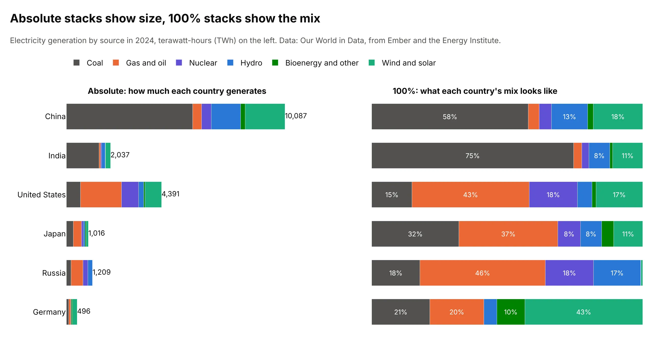
Data: Our World in Data, from Ember and the Energy Institute. A terawatt-hour (TWh) is a billion kilowatt-hours.
China's bar is 20 times as long as Germany's, so Germany's mix can't be read on the left, where its segments are slivers. On the right every country has the same length, and Germany's 43% from wind and solar and India's 75% from coal are plain. The cost is that the sizes are gone, so a 100% stack should always say somewhere what the totals are, in a label, a subtitle or a second chart. Use 100% when the totals are very different or don't matter (the vaccine, trial and jobs examples below), and absolute when they do.
Ordering the segments
The order of the segments decides what the reader can compare, because the first one is the only one on the baseline. It also decides whether the same source is in the same place in every bar. These are the same 100% bars in three orders:
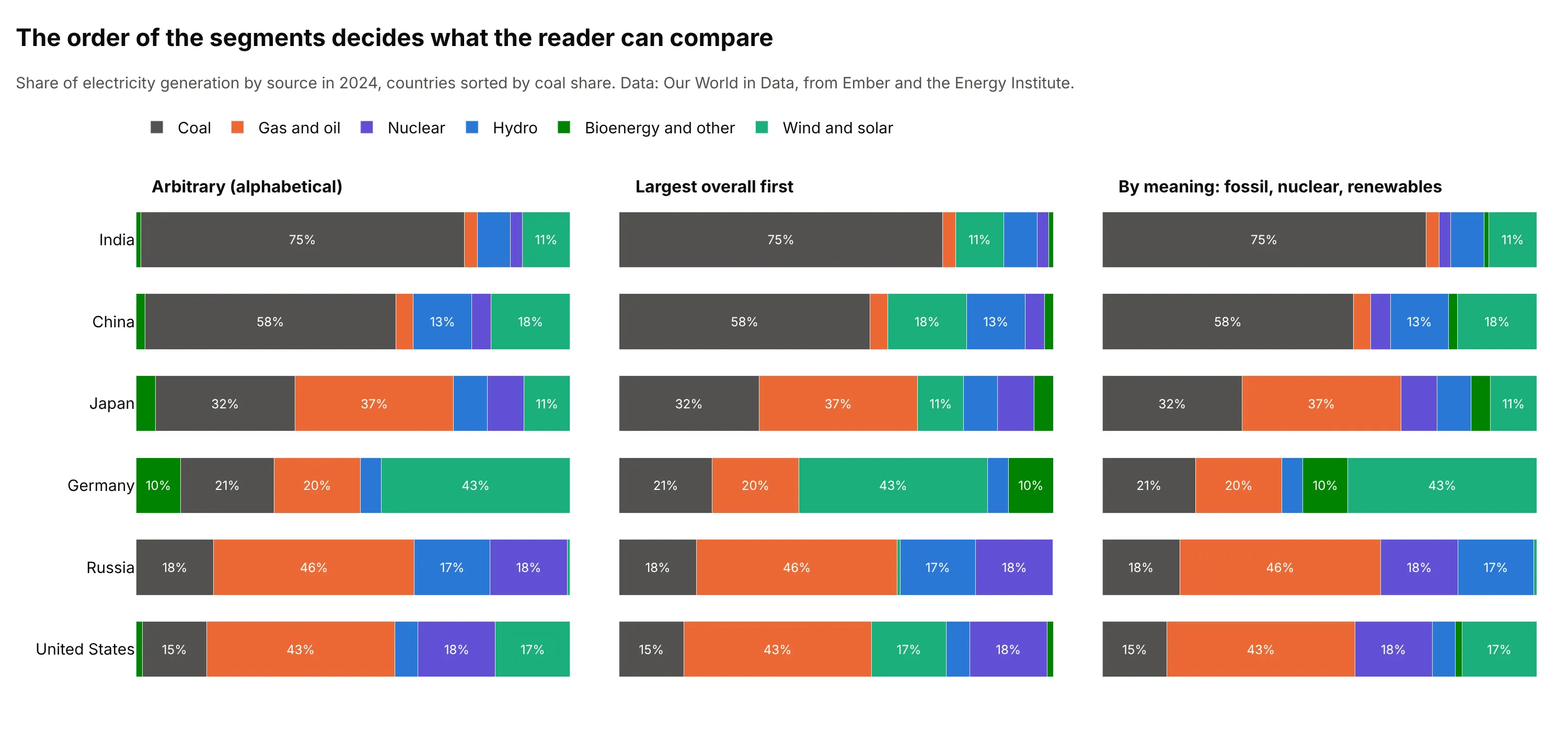
Data: Our World in Data, from Ember and the Energy Institute.
An arbitrary order such as alphabetical puts a small dark green bioenergy segment at the baseline in Germany and Japan, so the first segment isn't comparable across countries. The largest-first order helps a little, and the order by meaning (fossil fuels first, then nuclear and hydro, then newer renewables) tells a story, with coal and gas on the baseline and the renewables at the top. Some rules that work:
- Use the order the categories have. Phases of a trial, age groups, clarity grades and years run in one direction, and a stack should too, with one hue getting darker (the diamonds and trials examples).
- Otherwise put the biggest or the most important segment at the bottom, and keep that order, and the colors, the same in every bar and every chart.
- Match the legend to the stack. Plotly lists the traces of a stacked bar chart in reverse by default, so that a vertical legend reads top to bottom like the stack, so set legend.traceorder="normal" for a horizontal legend above the chart.
- Sort the bars, by total in an absolute stack or by the baseline segment in a 100% stack, unless they have a natural order like years.
Labeling totals
The total is often the point of a stacked bar, and Plotly doesn't print it, so add it. A bar trace's own text labels each segment, so the total needs an invisible text-only scatter trace at the top of each stack, as in the Python and JavaScript code below. The Federal Reserve example uses it for every column. Print the total in the same units as the axis, and for a horizontal stack put it at the end of the bar. In a 100% stack, print the totals in the row labels or the subtitle instead, and print the percentages inside the segments that are big enough, usually 6 to 7% or more, because a label that doesn't fit overlaps its neighbors.
Diverging stacks
An ordinary stack assumes that every part adds to the total. When some parts are negative, for example sources whose generation fell between two years, stacking them all upward makes no sense, and Wikipedia's bar chart article says stacked bar charts are not suited to data sets having both positive and negative values. A diverging stack, barmode="relative" in Plotly, stacks the positive values to the right of zero and the negative values to the left, and a marker for the net value shows what is left when the two sides cancel. Example 3 below uses it for the change in electricity generation since 2014, and the two charts here use it for trade and for a survey.
Trade in goods is a natural fit, because exports and imports are both positive numbers that point in opposite directions. This chart draws the exports of the European Union (EU) to its eight biggest trading partners to the right of zero and its imports from them to the left, with each side split by product group and a diamond for the net balance:
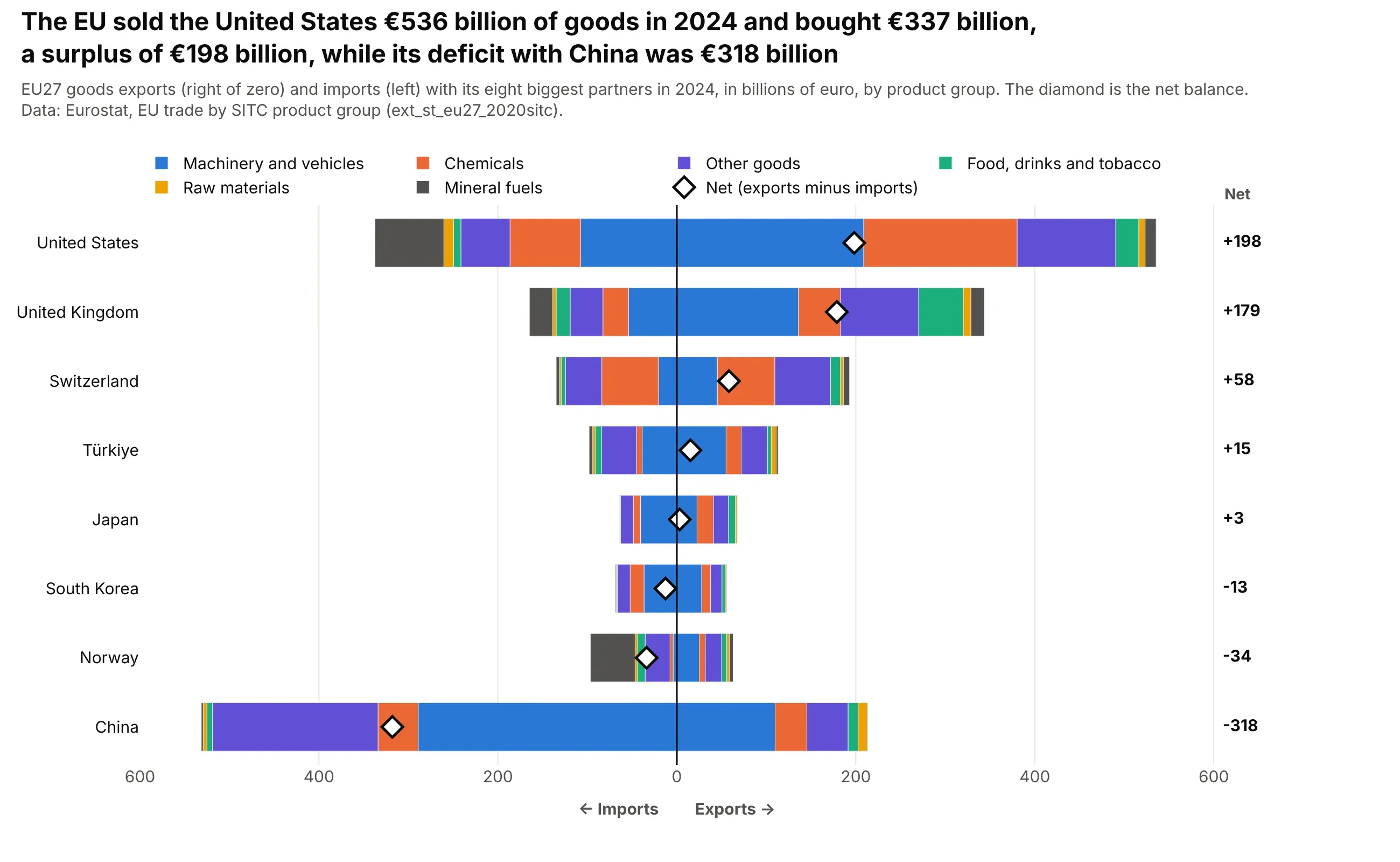
Data: Eurostat, EU trade in goods by product group (dataset ext_st_eu27_2020sitc), the 12 months of 2024 added up, in billions of euro.
The EU sold the United States €536 billion of goods in 2024 and bought €337 billion, so the diamond sits at +€198 billion, and the biggest segments on the import side are machinery and vehicles at €107 billion, chemicals at €79 billion and mineral fuels at €77 billion. China is the mirror image, with €213 billion of exports against €531 billion of imports, a net of -€318 billion, and most of the imports are machinery and vehicles (€289 billion) and other manufactured goods (€183 billion). The end of each side is a real total, all exports or all imports, and only the diamond shows the balance, which is why it needs to be on the chart. The code is short, because imports are drawn as negative values and barmode="relative" does the rest:
import pandas as pdimport plotly.graph_objects as gotrade = pd.read_csv("eu_trade.csv") # partner, product, exports, imports (billions of euro)colors = dict(zip(trade["product"].unique(), ["#2a78d6", "#eb6834", "#6250d6", "#1baf7a", "#eda100", "#52514e", "#a3a29b"]))fig = go.Figure()for product, part in trade.groupby("product"):# exports go right of zero, imports go left, and both sides use the same color for a productfig.add_bar(y=part.partner, x=part.exports, name=product, orientation="h", marker_color=colors[product], legendgroup=product)fig.add_bar(y=part.partner, x=-part.imports, orientation="h", marker_color=colors[product], legendgroup=product, showlegend=False)net = trade.groupby("partner")[["exports", "imports"]].sum().eval("exports - imports")fig.add_scatter(y=net.index, x=net, mode="markers", name="Net",marker=dict(symbol="diamond", size=14, color="white", line=dict(color="black", width=2)))fig.update_layout(barmode="relative")fig.show()
The same layout is how a Likert chart works for survey answers on an agree-to-disagree scale. This one shows how people in 11 EU countries and the EU average answered a question about the image they have of the EU, with the neutral answers split across zero so that the two sides show only the positive and the negative answers, and the neutral total in its own column:
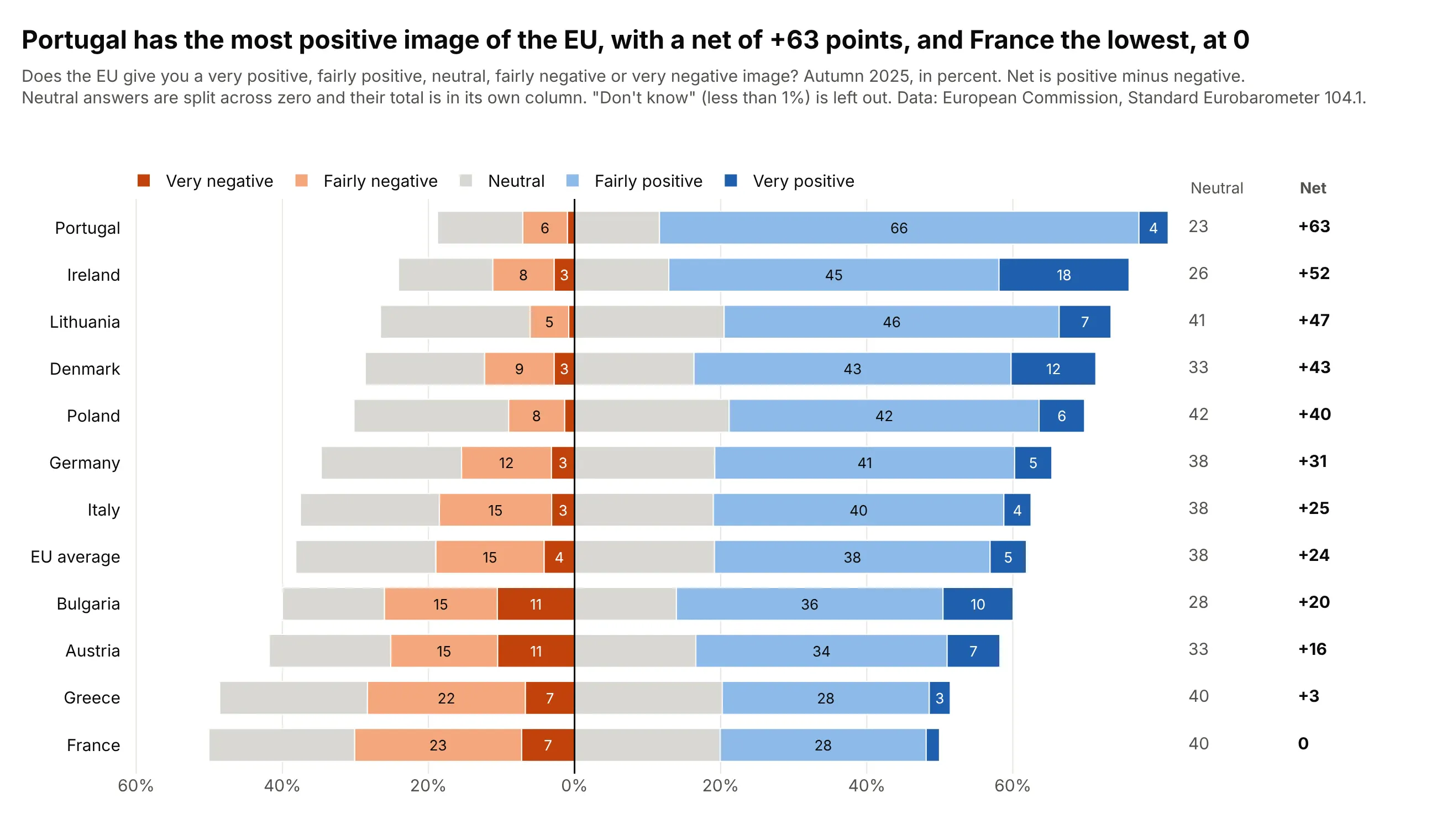
Data: European Commission, Standard Eurobarometer 104.1 (autumn 2025), the question on the image of the EU. "Don't know" answers (less than 1% in these countries) are left out and the rest is rescaled to 100%.
Portugal has the most positive image, with 66% fairly positive and 4% very positive against 7% negative, a net of +63 points, while France is at 0 because 30% are positive and 30% negative, and 40% are neutral. Splitting the neutral answers keeps the positive and negative sides on the same scale in every row, and the net column sorts the rows. See the Likert chart guide for the other ways to place the neutral answer, and the tornado chart guide for bars that diverge from a base case.
Grouped or stacked
A grouped bar chart puts the parts side by side, so every bar starts at zero and every part can be compared with every other. A stacked bar chart puts them on top of each other, so only the total and the bottom part can be compared well. The choice follows the question:
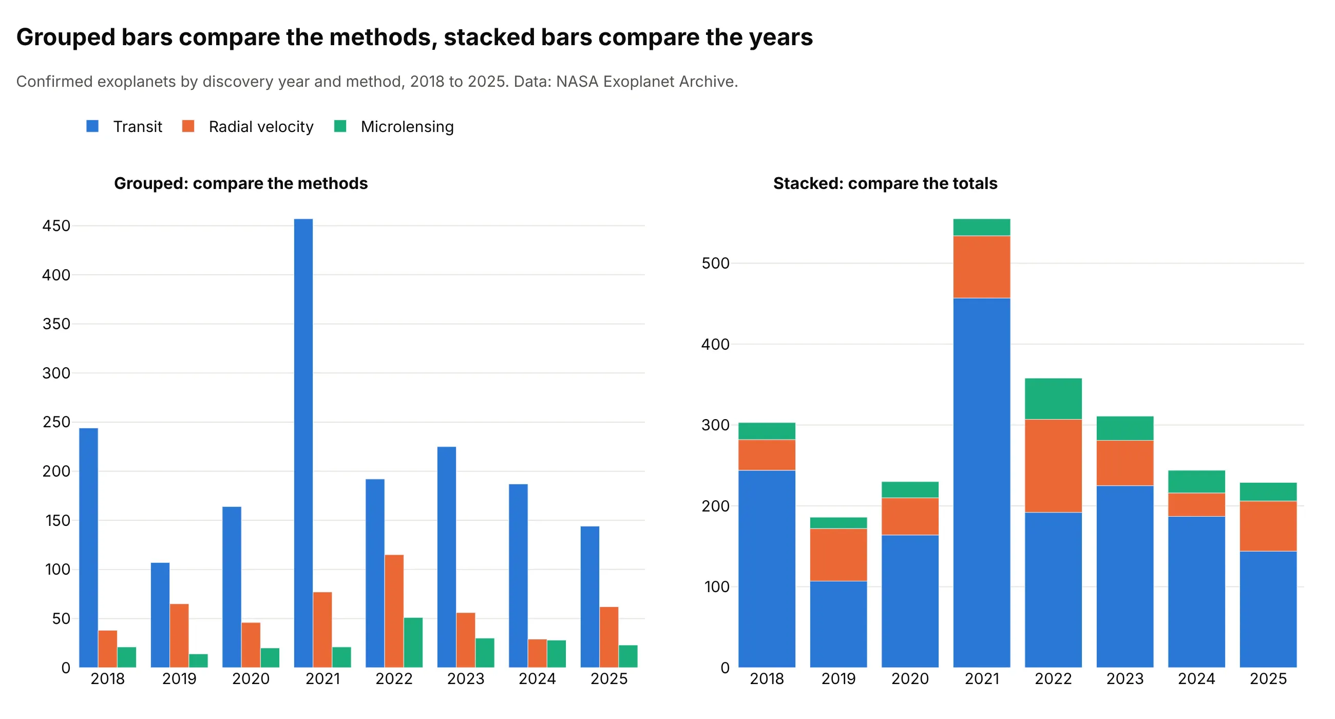
Data: NASA Exoplanet Archive, Planetary Systems Composite table.
Grouped bars answer "which method found the most?" without arithmetic, and the stacked bars answer "which year was the biggest?" at a glance, 555 planets in 2021 for these three methods. When both questions matter, a grouped and stacked bar chart puts two stacks side by side for each category, as the bar chart guide shows.
Variations of the stacked bar chart
The stacked bar chart belongs to a family of charts that show parts of a whole, and each relative changes one thing about it: the scale, the baseline, the width of the bars, the mark or the direction. This figure draws the same data, the share of electricity generation by source in 2024 for six countries, in three of those ways, and the sections after it show the others:
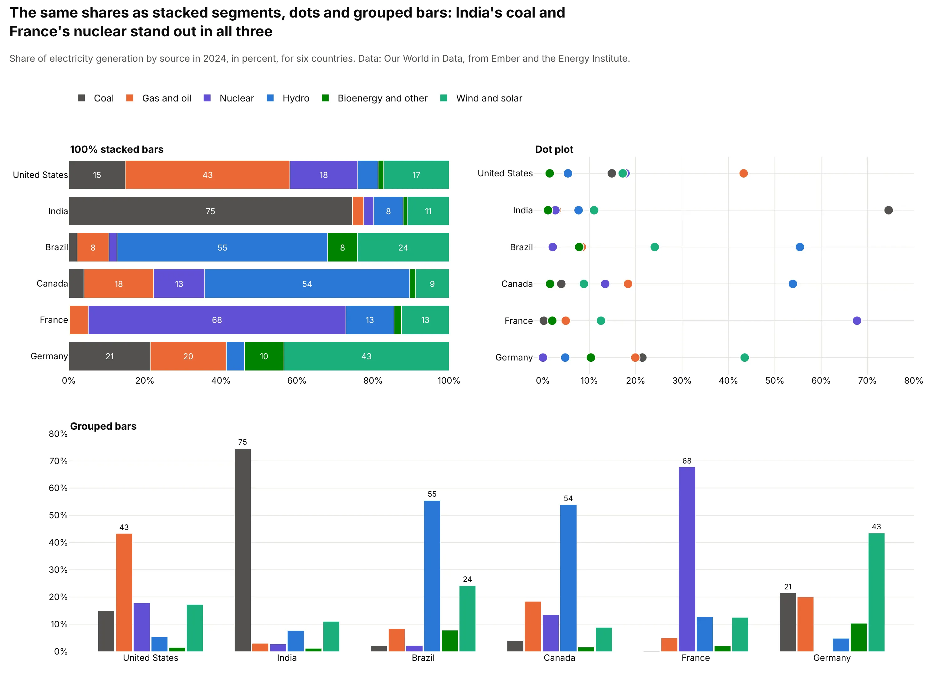
Data: Our World in Data, from Ember and the Energy Institute.
- 100% stacked bars (the mix, without the size). Every bar has the same length, so India's 75% coal and France's 68% nuclear are visible at once, while the totals disappear (see "Absolute or 100%" above). Pick it when the mix matters more than the size.
- Dot plot (each part on a common scale). The dot plot puts every share on one axis from zero, so Brazil's 55% hydro and Canada's 54% can be compared directly, which the upper segments of a stack don't allow. It gives up the feeling that the parts add up to a bar, so pick it when the reader needs to compare one part across rows or when there are more parts than a stack can show.
- Grouped bars (every part from zero). Each part gets its own bar, so the biggest source in each country is clear without arithmetic, as in "Grouped or stacked" above. The whole is lost, and 36 bars already crowd this panel, so pick it for few categories when the parts are the question.
- Diverging stacked bars and the Likert chart (parts with two directions). These put negative parts to the left of zero and positive parts to the right, as in the trade and survey charts in "Diverging stacks" above. Pick them when the parts have opposite signs or opposite meanings, such as exports and imports or agree and disagree.
Marimekko chart
A Marimekko chart, also called a mosaic chart, is a 100% stacked bar chart whose columns have widths in proportion to a second quantity, so the area of each block shows the amount. Here the width is each country's total generation, which shows that the United States column is nine times as wide as Germany's and that its 43% of gas and oil is the largest block on the chart:
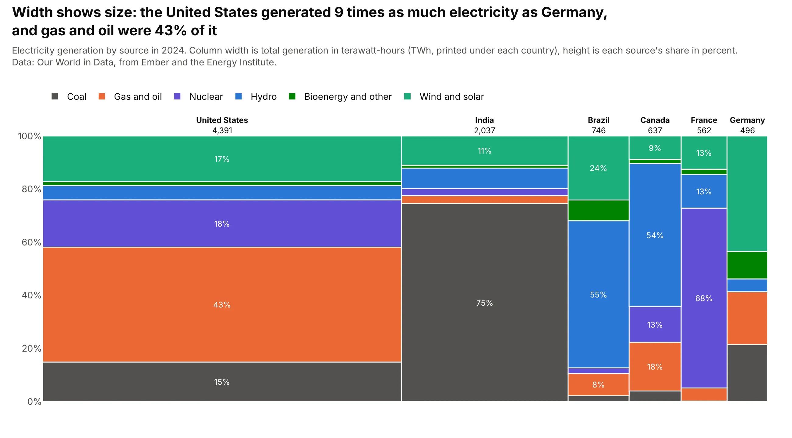
Data: Our World in Data, from Ember and the Energy Institute.
Pick a Marimekko chart for two categorical variables and one measure, such as market share by region and segment, when both the size of each group and its mix matter. The blocks in narrow columns are hard to label, so it works best with about six columns or fewer.
Waffle chart
A waffle chart turns a 100% stack into a grid of 100 squares, one for each percent, so the reader counts the parts instead of measuring them. The squares are rounded so that they add to 100, which gives Germany 44 squares of wind and solar from a share of 43.5%:
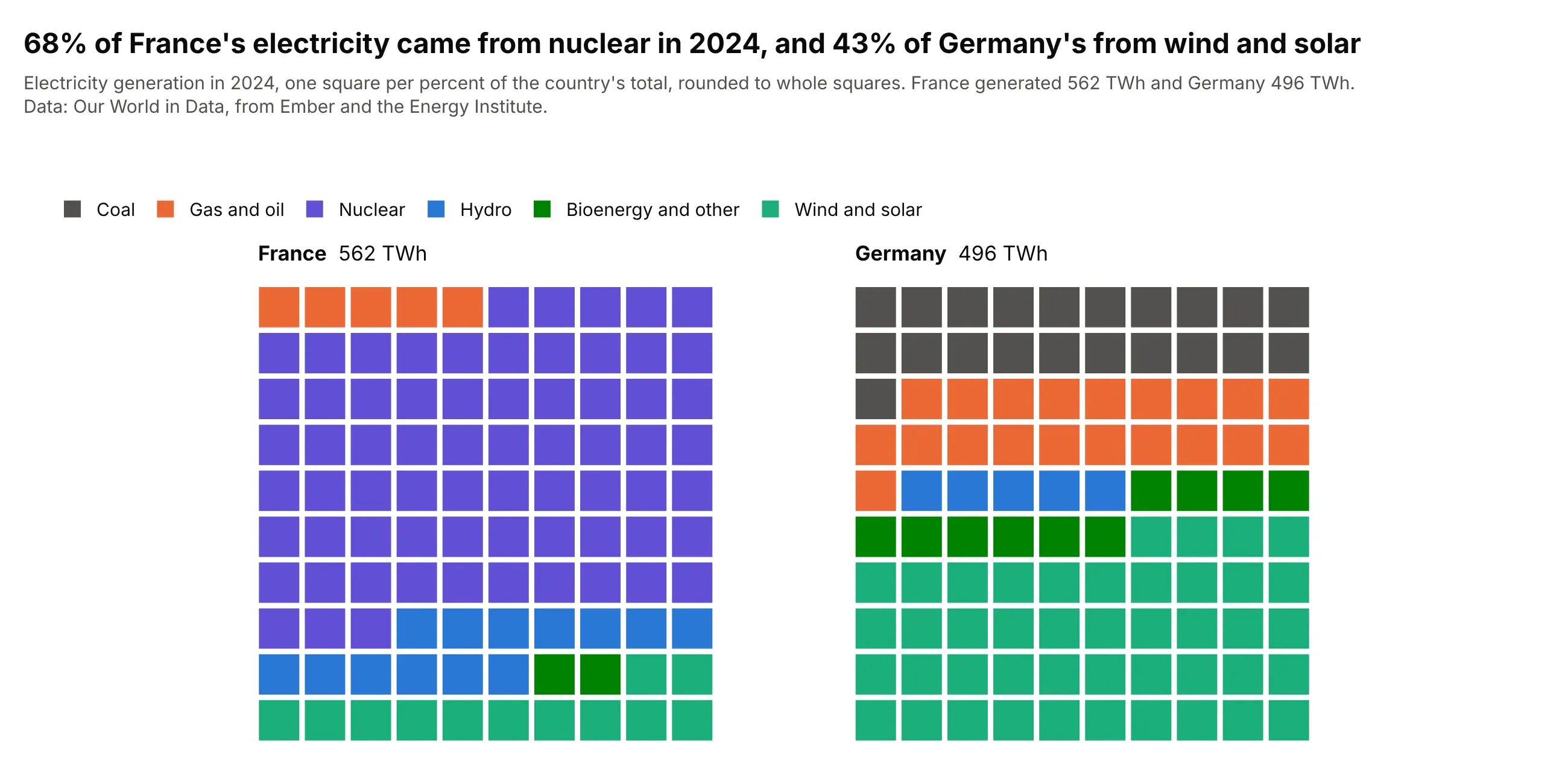
Data: Our World in Data, from Ember and the Energy Institute.
It is easy to read for one or two wholes with a handful of parts, such as France's 68 squares of nuclear. It doesn't suit many bars or shares under 1%, which are less than one square.
Stacked area chart
A stacked area chart is a stacked bar chart for continuous time, with each part drawn as a filled band, so the top edge is the total and the thickness of a band is its value. In the United States data the coal band at the bottom thins from 1,966 TWh in 2000 to 737 TWh in 2025 while the wind and solar band at the top grows from 6 to 853:
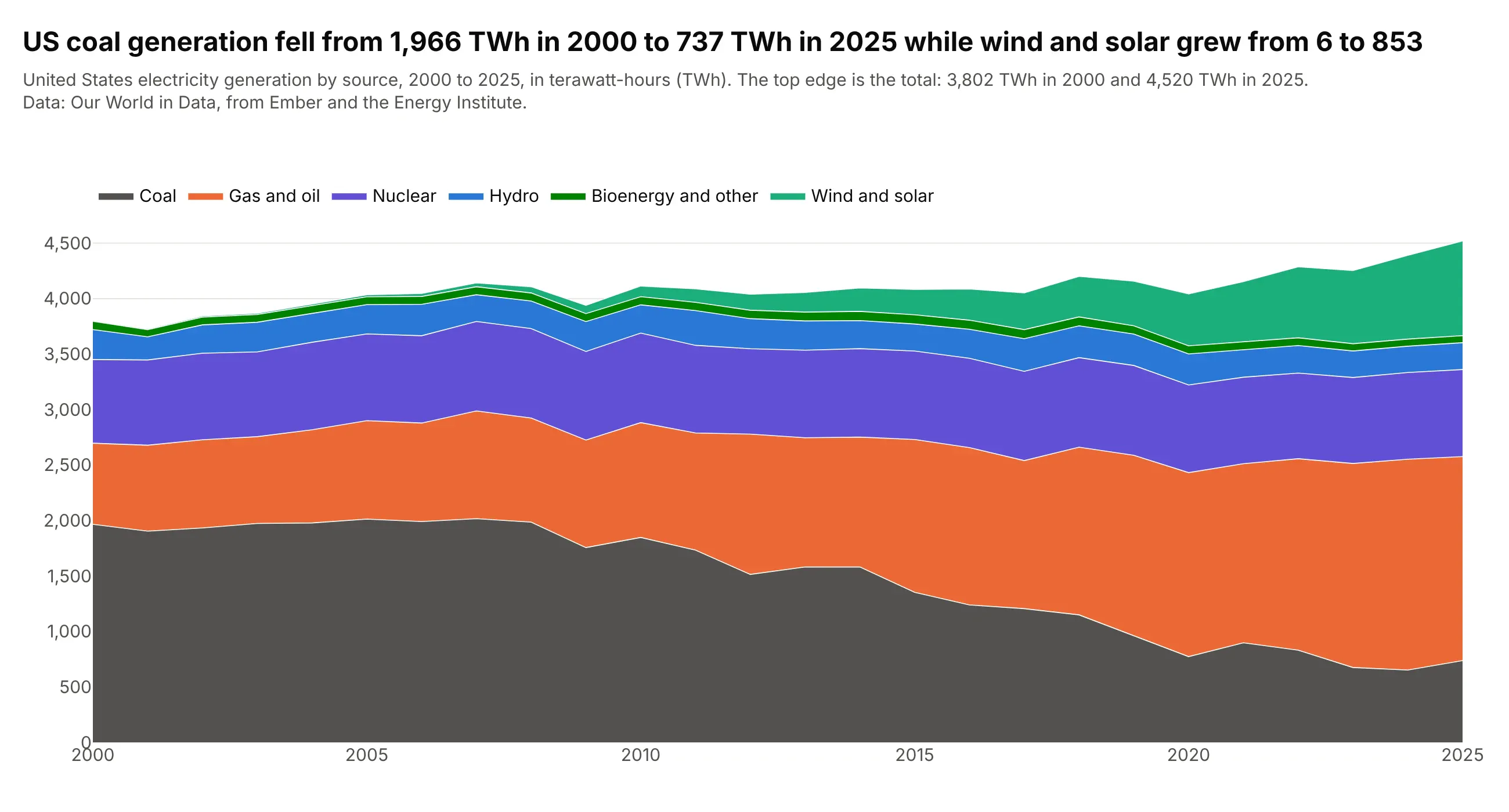
Data: Our World in Data, from Ember and the Energy Institute.
It has the same baseline problem as a stack, because only the bottom band starts at zero, and it is the better choice when there are many time points, where a column for every year becomes a comb. A streamgraph floats the baseline in the middle so that the bands are easier to follow.
Population pyramid
A population pyramid is a diverging stacked bar chart for two groups, with men to the left and women to the right of zero and one bar for each age group, so both sides are positive counts, as in the trade chart. The shape shows the age structure at once, and in Japan the largest bar is 8.2 million women aged 80 and over, against 4.9 million men:
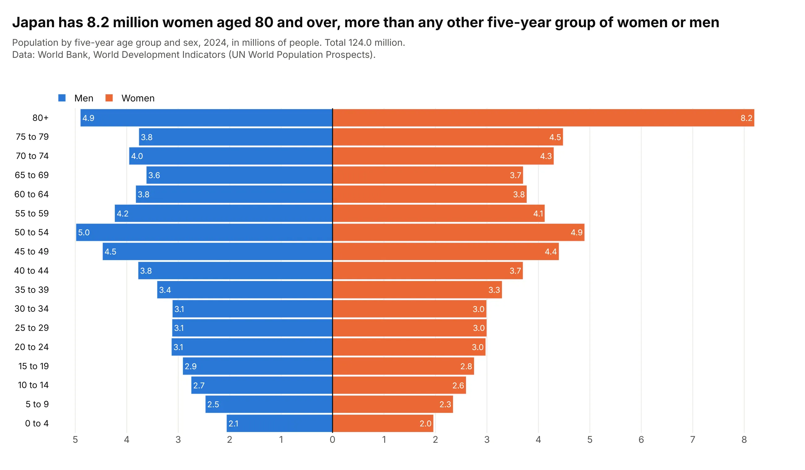
Data: World Bank, World Development Indicators (UN World Population Prospects), 2024.
Pick it when two groups are compared along an ordered scale such as age, and each side adds up to a total on its own.
Other relatives
A treemap packs the parts into nested rectangles, which fits when there are dozens of parts or a hierarchy, and a dumbbell chart shows the change in one part between two points in time as a line between two dots, which is clearer than two stacks when the question is how much each part changed.
Alternatives to a stacked bar chart
Here's the same United Kingdom electricity data drawn six ways. Some are better for the question, some worse, some just different:
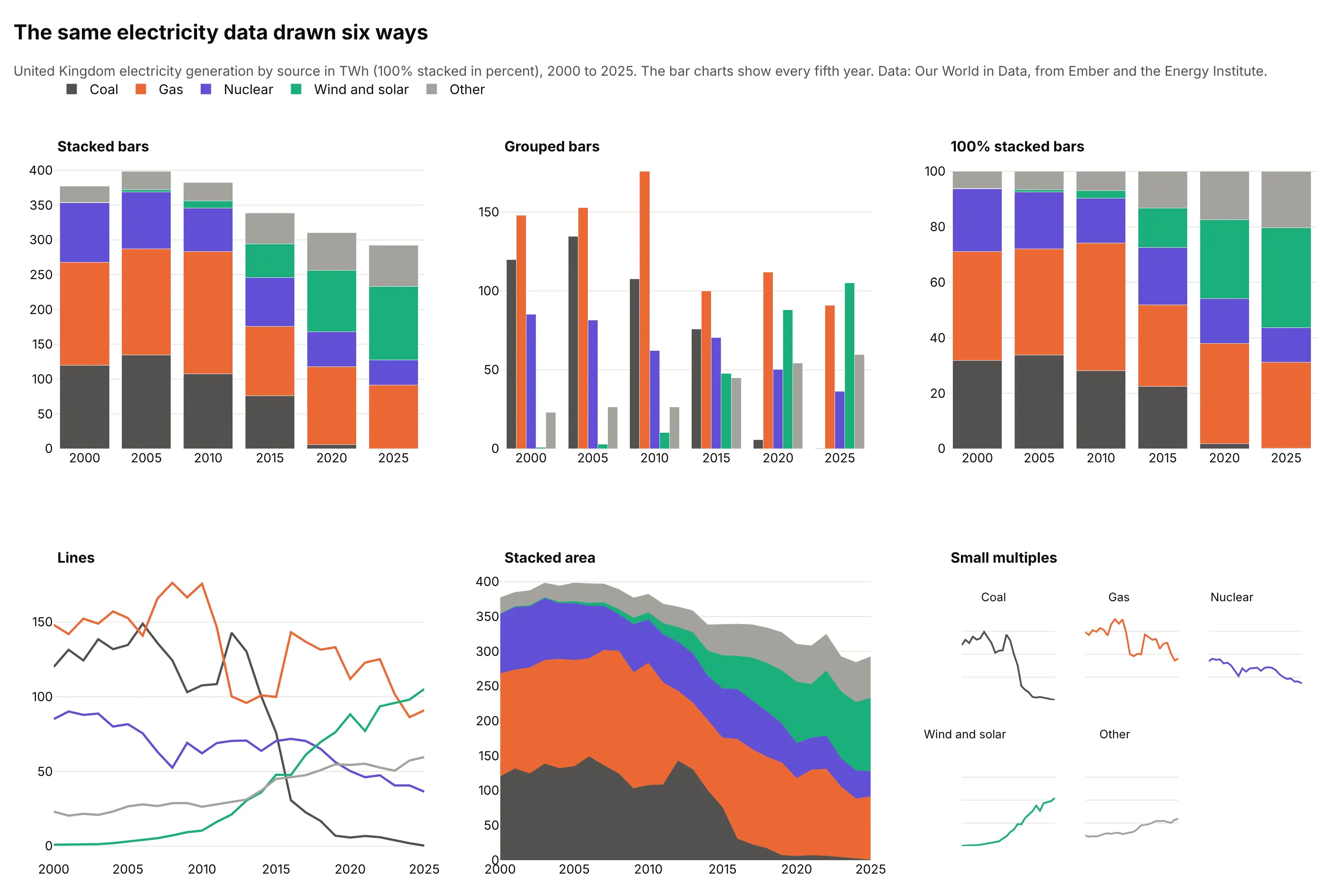
Data: Our World in Data, from Ember and the Energy Institute.
- Stacked bars (works for totals and the bottom part). The total fell from 377 TWh in 2000 to 292 TWh in 2025, and the bottom part, coal, fell from 120 to 0.3. The sources above it are harder to follow.
- Grouped bars (better for comparing the parts). Gas's 176 TWh peak in 2010 is easy to compare with nuclear's 62, but the total isn't visible and the sources are repeated six times.
- 100% stacked bars (better for the mix). Wind and solar went from 0.2% to 36%, a share that the absolute stacks hide because the total shrank.
- Line chart (better for trends of each part). Coal falling and wind and solar rising cross in 2016, when wind and solar first exceeded coal, and can be followed one by one, but the total is gone.
- Stacked area chart (works too for continuous time). It keeps the total and the stack, with the same baseline problem (see "Variations of the stacked bar chart" above).
- Small multiples (better for many parts). One small chart per source, on the same scale, with no baseline problem at all.
For a whole made of a few parts at one point in time, a pie chart works, and a ternary plot shows three parts at once. The Marimekko chart, waffle chart and dot plot are covered under "Variations of the stacked bar chart" above.
How to make a stacked bar chart
With AI
ChatGPT, Claude Code, GitHub Copilot, Cursor and other AI tools are excellent at writing Plotly code. Name Plotly in the prompt, and say whether the stack is absolute or 100%, which segment goes at the bottom, and whether to label the totals:
Make a plotly stacked bar chart from exoplanets.csv (columns: year, method, planets).- One column per year, 2018 to 2025, one bar trace per method, stacked with barmode="stack".- Stack order: Transit at the bottom, then Radial velocity, then Microlensing; the same colors in every column.- Print each year's total above its column with a text-only scatter trace.- Legend above the plot in stack order (legend traceorder "normal"), white background, thousands separators on the axis.- Check: print the total for each year.
With Plotly Studio
Plotly Studio is a product for creating data visualizations and Dash apps and for analyzing data with AI, available as a desktop app or embedded in Dash apps. Ask for a stacked bar chart the same way:
Show a stacked bar chart of planets confirmed per year by discovery method, with the total above each column, a toggle between absolute counts and percent, and a dropdown to pick the first year.
Make a stacked bar chart in Python or JavaScript
This is the code AI tools write under the hood. In Python, Plotly Express stacks by default (px.bar uses barmode="relative", which also stacks negative values below zero), so one line is enough for a first version:
import pandas as pdimport plotly.express as pxdf = pd.read_csv("exoplanets.csv") # year, method, planetsfig = px.bar(df, x="year", y="planets", color="method") # stackedfig.update_layout(barnorm="percent") # 100% stackedfig.show()
For a chart you can publish, this helper takes a table with one row per bar and one column per segment, puts the first column at the bottom and prints the totals. It returns a go.Figure:
import pandas as pdimport plotly.graph_objects as godef stacked_bar(wide, colors=None, percent=False, totals=True):"""A stacked bar chart in Plotly: one bar trace per column (the first column is the bottom segment) and,for an absolute chart, the total above each stack."""fig = go.Figure()for col in wide.columns:fig.add_bar(x=wide.index, y=wide[col], name=col, marker_color=(colors or {}).get(col))fig.update_layout(barmode="stack", barnorm="percent" if percent else None, template="simple_white",legend=dict(orientation="h", y=1.1, traceorder="normal"))if totals and not percent:total = wide.sum(axis=1)fig.add_scatter(x=wide.index, y=total, mode="text", text=[f"{t:,.0f}" for t in total],textposition="top center", showlegend=False, hoverinfo="skip")return figdf = pd.read_csv("exoplanets.csv") # year, method, planetstop = ["Transit", "Radial Velocity", "Microlensing"] # bottom segment firstwide = (df[df.year.between(2018, 2025) & df.method.isin(top)].pivot_table(index="year", columns="method", values="planets", aggfunc="sum", fill_value=0)[top])fig = stacked_bar(wide, {"Transit": "#2a78d6", "Radial Velocity": "#eb6834", "Microlensing": "#1baf7a"})fig.show()
For a diverging stack, pass positive and negative columns and use barmode="relative". In JavaScript, plotly.js draws the same chart with three bar traces and one text trace:
<div id="chart"></div><script src="https://cdn.plot.ly/plotly-4.1.1.min.js"></script><script>// Confirmed exoplanets by discovery year and method, 2018 to 2025 (NASA Exoplanet Archive)const years = [2018, 2019, 2020, 2021, 2022, 2023, 2024, 2025];const transit = [244, 107, 164, 457, 192, 225, 187, 144];const radial = [38, 65, 46, 77, 115, 56, 29, 62];const micro = [21, 14, 20, 21, 51, 30, 28, 23];const totals = years.map((_, i) => transit[i] + radial[i] + micro[i]);Plotly.newPlot("chart", [{type: "bar", x: years, y: transit, name: "Transit", marker: {color: "#2a78d6"}},{type: "bar", x: years, y: radial, name: "Radial velocity", marker: {color: "#eb6834"}},{type: "bar", x: years, y: micro, name: "Microlensing", marker: {color: "#1baf7a"}},{type: "scatter", mode: "text", x: years, y: totals, text: totals.map(String), textposition: "top center",showlegend: false, hoverinfo: "skip"}], {width: 900, height: 450, barmode: "stack", // "relative" for positive and negative values; add barnorm: "percent" for 100%legend: {orientation: "h", y: 1.12, traceorder: "normal"},xaxis: {dtick: 1}, yaxis: {title: {text: "Planets confirmed"}, range: [0, 620]}});</script>
Share it
Every Plotly chart has a Share chart button (the cloud icon in its toolbar) that uploads it to Plotly Cloud and gives you a link. Only you can see it until you change its visibility.
For a live app, put the chart in a Dash app and publish it with the Plotly Cloud CLI. Coding agents can run these commands for you:
pip install "dash[cloud]"plotly user loginplotly app publish
If your data has to stay in your own cloud or data center, publish to Dash Enterprise instead.
Dos and don'ts
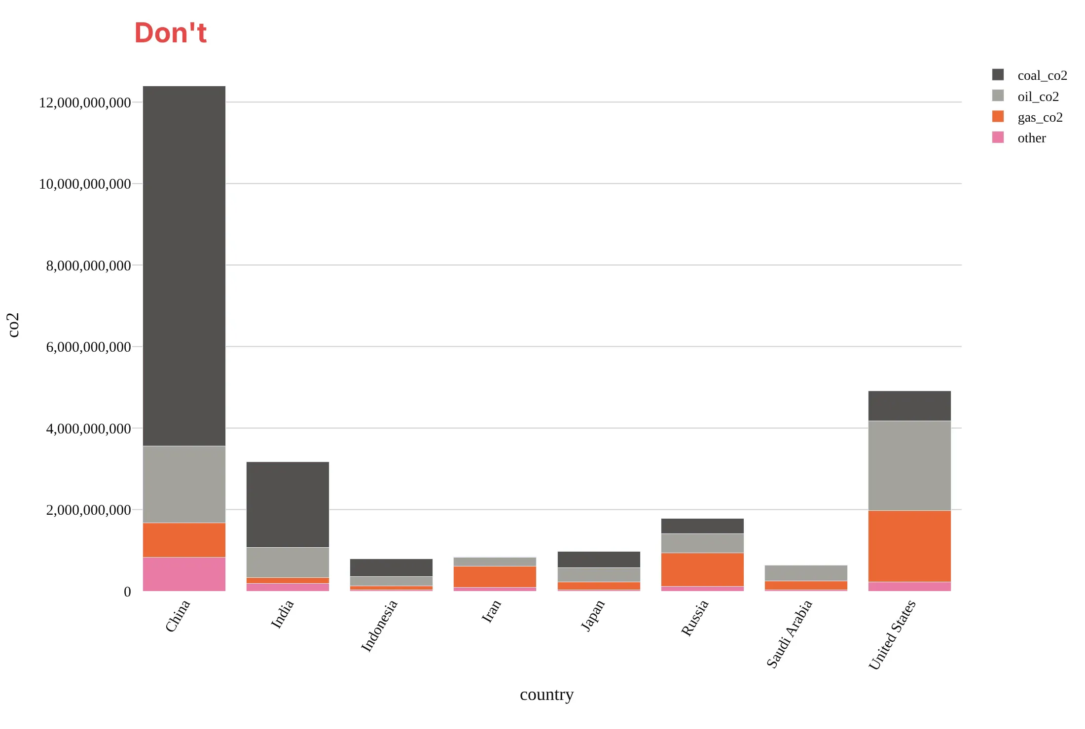
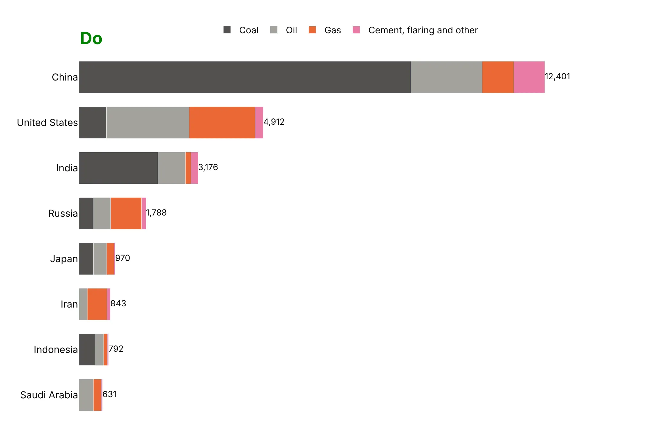
Most of the work in a good stacked bar chart is deciding the order and the totals, and then removing the clutter. Here are the 2024 carbon dioxide emissions of the eight largest emitters, drawn both ways in the same colors.
Don't leave the countries in alphabetical order, put the segments in an order with no logic (the smallest at the bottom, where the baseline is wasted on it), leave the totals unprinted, show raw column names in the legend and unformatted billions on the axis, use a serif font, or rotate the country names:
Do sort the bars by total, make them horizontal so that the names read, put the segment that matters at the baseline, keep the segments in a stable order that matches the legend, and print each total at the end of its bar:
Checklist
Do
- Stack only when the total is meaningful, and say what it is.
- Put the most important segment at the bottom, and keep the order and the colors the same in every bar.
- Use a natural order when the parts have one, with one hue from light to dark.
- Print the totals, and the values inside segments big enough to hold them.
- Group small segments into "Other", and keep the stack to about five segments.
- Start the value axis at zero, and use a 100% stack when the mix matters more than the size.
Don't
- Don't stack parts that don't add up to a meaningful total, such as rates or percentages of different bases.
- Don't compare upper segments by eye when the difference matters, and give them printed values or use grouped bars.
- Don't mix positive and negative values in one ordinary stack, and use a diverging stack.
- Don't use a different color for the same part in different charts or let the legend order contradict the stack.
- Don't use more colors than the reader can match to a legend, and don't use a rainbow for ordered parts.
More stacked bar chart examples
1. Vaccine doses by manufacturer in 100% stacked bars
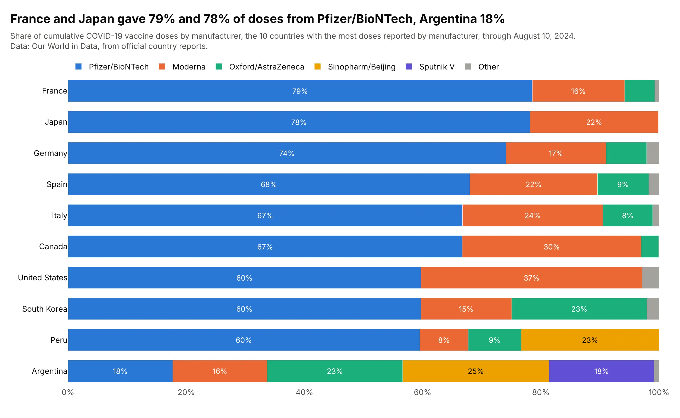
France gave 79% of its COVID-19 vaccine doses from Pfizer/BioNTech and Japan 78%, while Argentina's 18% was spread over five manufacturers. Country totals differ by a factor of almost 8 (672.6 million doses in the United States, 87.5 million in South Korea), so the 100% stack compares the mix and leaves out the size. Data: Our World in Data, from official country reports, through August 10, 2024.
Tip: sort the rows by the baseline segment, so the one comparison the stack allows, Pfizer/BioNTech's share, becomes a ranking.
Get the data from Our World in Data's COVID-19 vaccine doses by manufacturer(ourworldindata.org/grapher/covid-vaccine-doses-by-manufacturer.csv, cumulative doses by manufacturer percountry and day) and shape it into a table with the last reported day for the 10 countries with the most doses(columns: country, manufacturer, doses).Build a plotly horizontal 100% stacked bar chart (barmode="stack", barnorm="percent") sorted by the Pfizer/BioNTechshare, small manufacturers grouped as Other, and the percentage printed in segments of 7% or more.
2. World carbon dioxide emissions by source
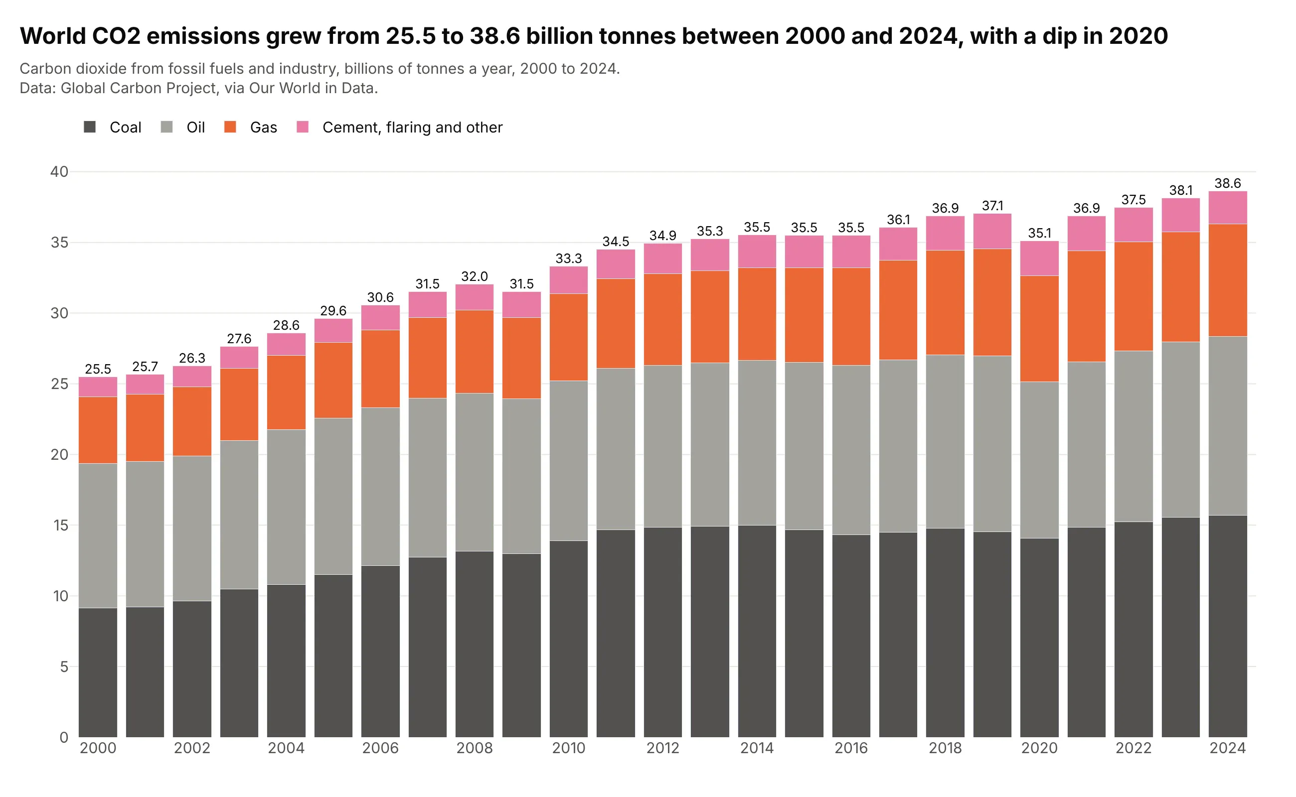
World carbon dioxide emissions grew 52% between 2000 and 2024, from 25.5 to 38.6 billion tonnes, and fell 5.3% in 2020, to 35.1 billion tonnes from 37.1 in 2019. Coal sits on the baseline at 15.7 billion tonnes in 2024, about 41% of the total, so its slow growth is the easy part to read. Data: Global Carbon Project, via Our World in Data.
Tip: when the baseline segment is the story, use a neutral dark color for it, and keep brighter colors for the parts above.
Get the data from Our World in Data's CO2 dataset (github.com/owid/co2-data, owid-co2-data.csv, the World rows2000-2024, columns coal_co2, oil_co2, gas_co2, cement_co2, flaring_co2, other_industry_co2 and co2 in milliontonnes) and shape it into a table (columns: year, source, gigatonnes).Build a plotly stacked bar chart, one column per year, coal at the bottom, then oil, gas and a combined cement,flaring and other segment, with each year's total printed above the column.
3. Change in electricity generation by source
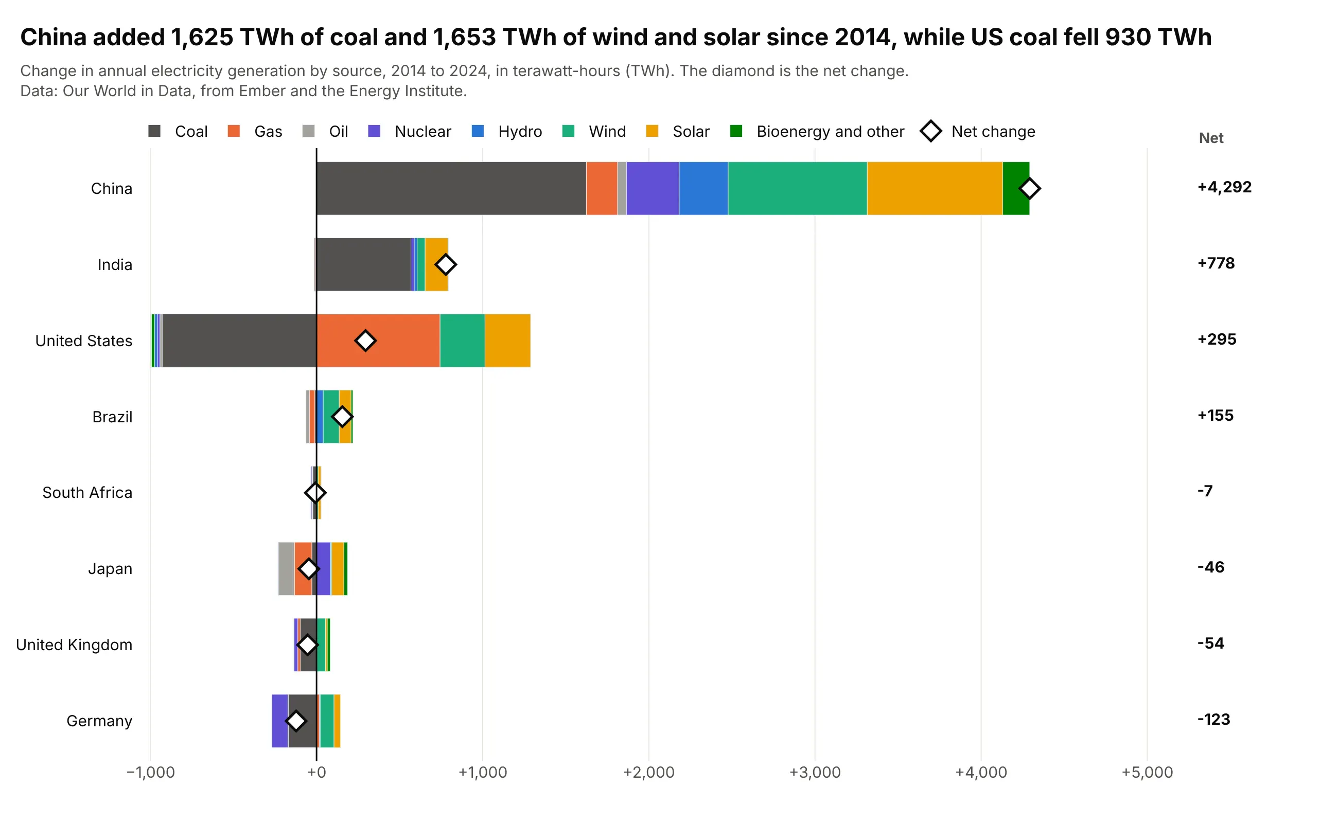
China added 1,625 TWh of coal-fired generation and 1,653 TWh of wind and solar between 2014 and 2024, a net change of +4,292 TWh, while US coal fell 930 TWh and gas rose 743. With barmode="relative" the rises stack to the right of zero and the falls to the left, and the diamond shows the net change. Data: Our World in Data, from Ember and the Energy Institute.
Tip: print the net value in a separate column at the right edge, because labels next to the diamonds collide with short bars.
Get the data from Our World in Data's energy dataset (github.com/owid/energy-data, owid-energy-data.csv,columns coal_electricity, gas_electricity, oil_electricity, nuclear_electricity, hydro_electricity,wind_electricity, solar_electricity, biofuel_electricity in TWh) and shape it into a table with the change from2014 to 2024 for China, India, the United States, Germany, the United Kingdom, Japan, Brazil and South Africa(columns: country, source, change_twh).Build a plotly horizontal diverging stacked bar chart with barmode="relative", countries sorted by net change,one color per source, a diamond marker for each country's net change and its value in a column at the right.
4. One household's electricity use by circuit
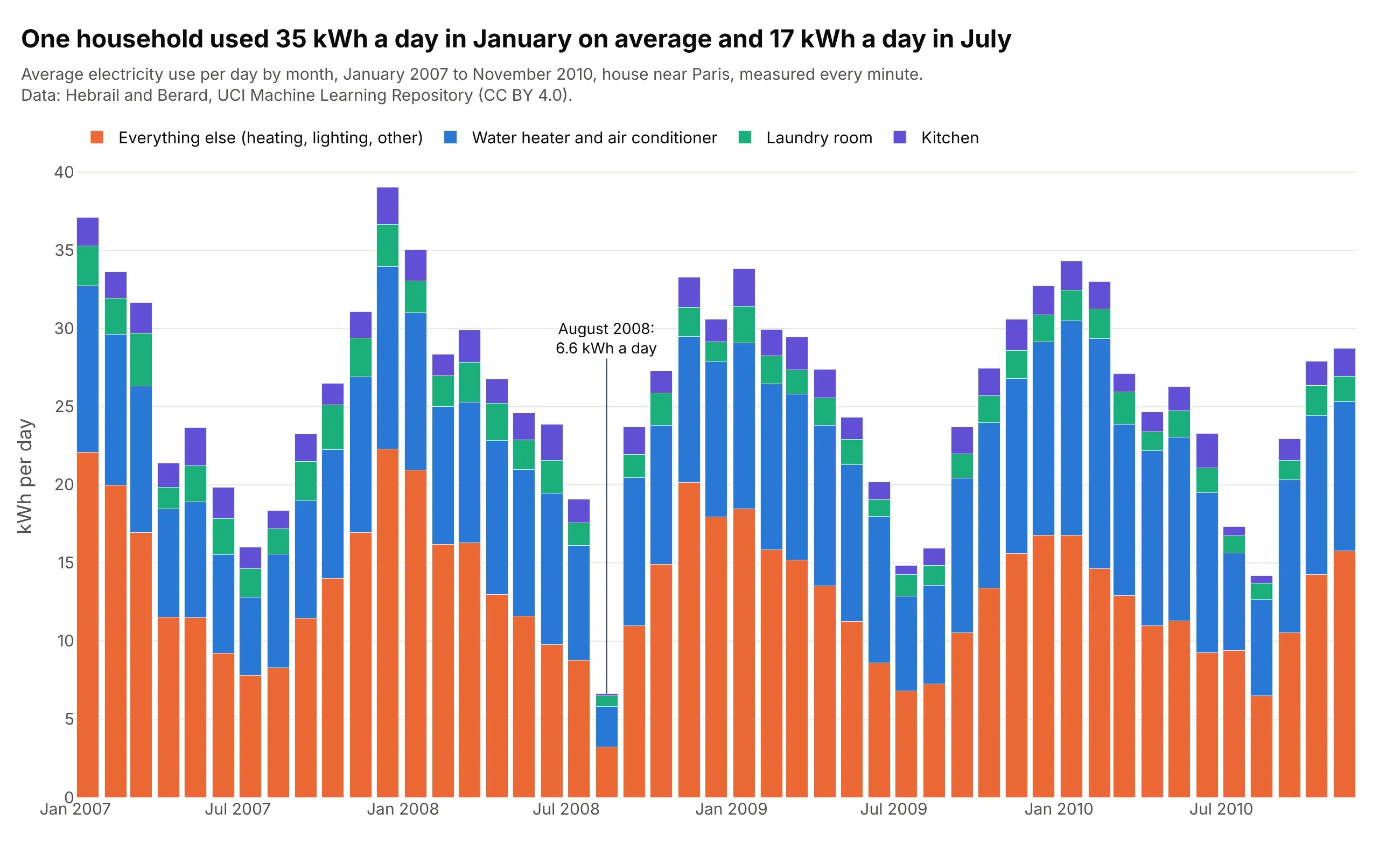
The household used 35 kWh (kilowatt-hours) a day in January and 17 in July on average, and the remainder after the three sub-meters (heating, lighting and everything else) went from 19.6 to 8.2, which is 11.4 of the 18.3 kWh a day swing. August 2008 is the low month, at 6.6 kWh a day. Data: Hebrail and Berard, UCI Machine Learning Repository, one reading per minute.
Tip: convert monthly sums to an average per day, so that months of different length, and months with missing readings, compare fairly.
Get the data from the UCI Machine Learning Repository's "Individual household electric power consumption"dataset (archive.ics.uci.edu/dataset/235, one reading per minute from December 2006 to November 2010, columnsGlobal_active_power, Sub_metering_1, Sub_metering_2 and Sub_metering_3) and shape it into a table with one rowper month (columns: month, kitchen, laundry, water_heater_ac, other, in kWh per day, where other is the totalactive energy minus the three sub-meters and minutes with missing values are dropped).Build a plotly stacked bar chart of the four columns by month, other at the bottom, and label the lowest month.
5. Objects launched into space by country
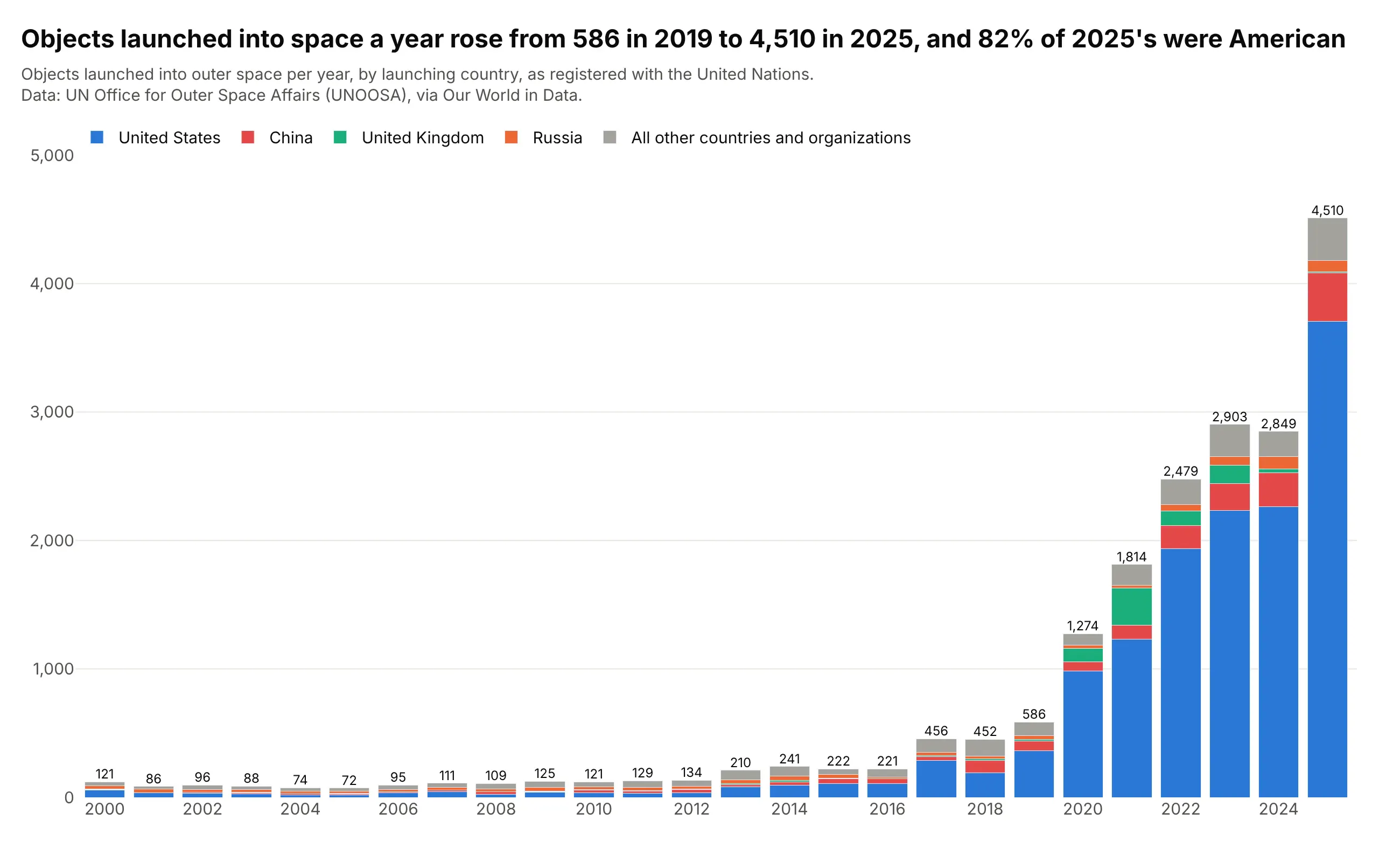
Objects launched into space a year rose from 586 in 2019 to 4,510 in 2025, and the United States was 82% of the 2025 total, up from 62% in 2019. With the United States on the baseline, its share of the growth is the thing the eye follows. Data: UN Office for Outer Space Affairs (UNOOSA), via Our World in Data.
Tip: when one segment dominates, give it the baseline and a strong color, and let the others share a quiet one.
Get the data from Our World in Data's "Yearly number of objects launched into outer space"(ourworldindata.org/grapher/yearly-number-of-objects-launched-into-outer-space.csv, from the UN Office for OuterSpace Affairs) and shape it into a table for 2000-2025 (columns: year, country, objects) with the World row asthe total.Build a plotly stacked bar chart with the United States at the bottom, then China, the United Kingdom, Russia andthe rest, and the World total printed above each column.
6. Clinical trial phases by condition
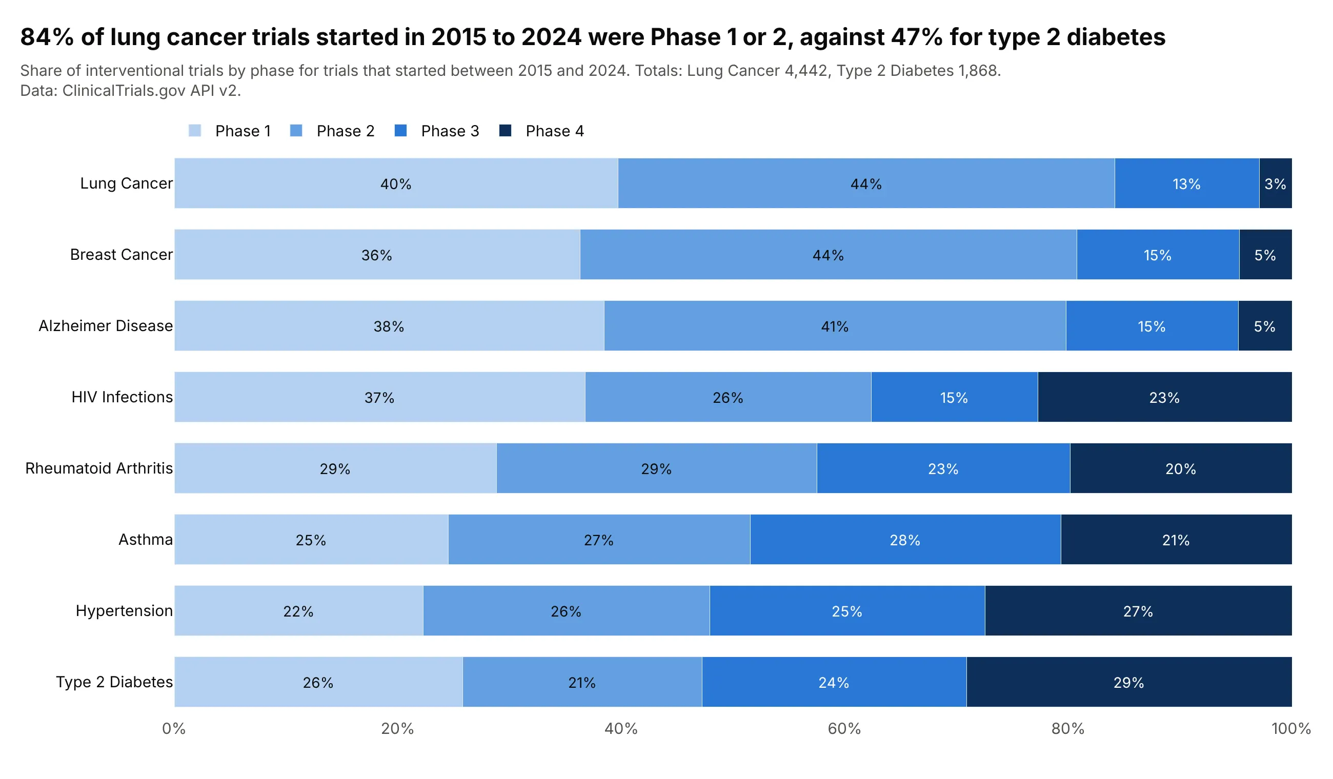
84% of the 4,442 lung cancer trials that started between 2015 and 2024 were Phase 1 or Phase 2, against 47% of the 1,868 type 2 diabetes trials. The phases have an order, so the stack runs from Phase 1 to Phase 4 in one hue, and the baseline segment says how early each field's pipeline is. Data: ClinicalTrials.gov API v2.
Tip: for ordered categories use one hue from light to dark instead of a rainbow, so that the order is visible without the legend.
Get the data from the ClinicalTrials.gov API v2 (clinicaltrials.gov/api/v2/studies with countTotal=true,interventional trials with a start date from 2015-01-01 to 2024-12-31, condition searches for breast cancer,lung cancer, type 2 diabetes, Alzheimer disease, asthma, HIV infections, rheumatoid arthritis and hypertension)and shape it into a table of counts (columns: condition, phase, trials) with Phase 1 including Phase 1/2, Phase 2including Phase 2/3 and early Phase 1 and trials without a phase left out.Build a plotly horizontal 100% stacked bar chart sorted by the Phase 1 plus Phase 2 share, in four shades ofblue from Phase 1 to Phase 4, with the percentage printed in each segment.
7. US jobs by sector
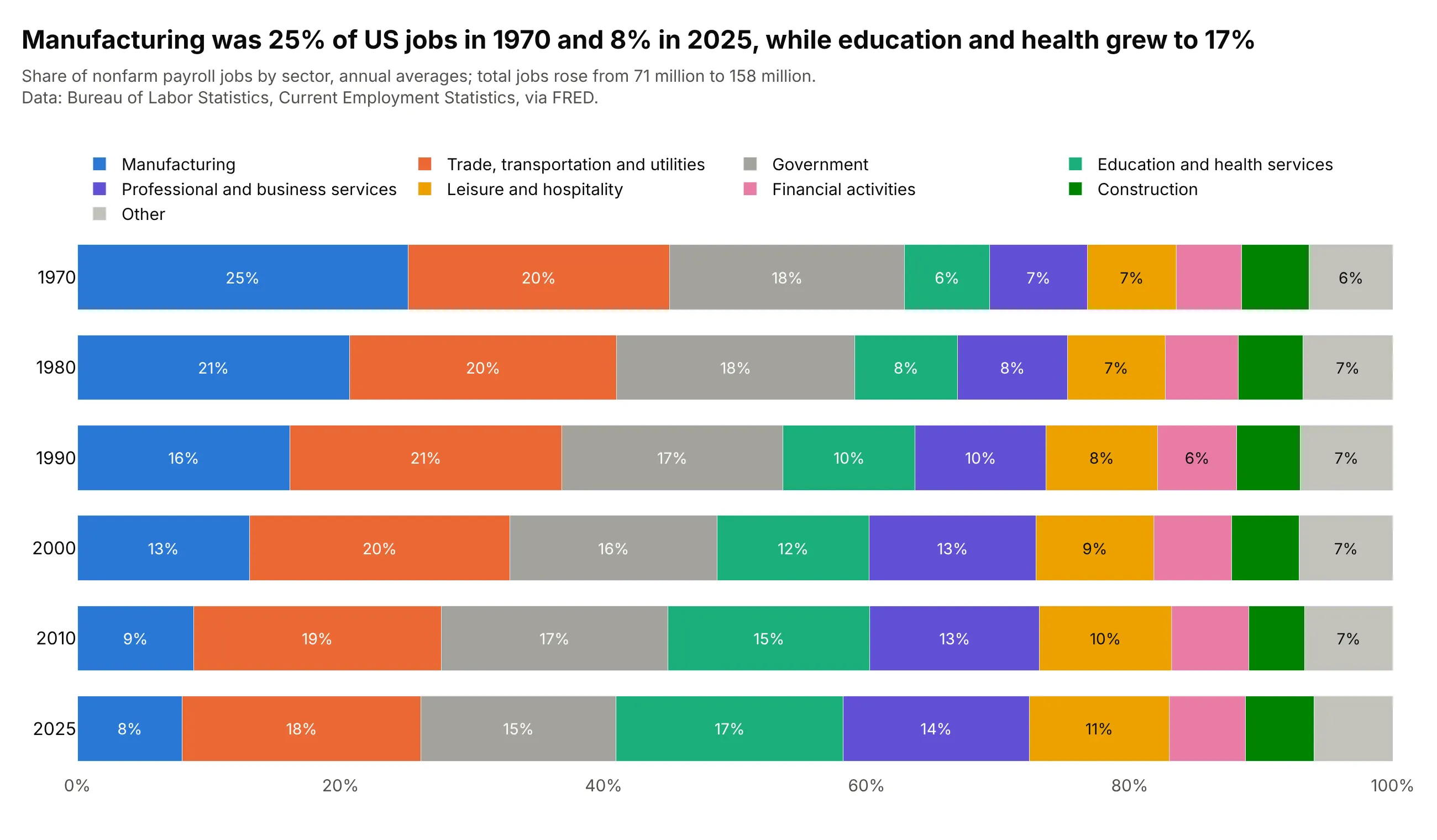
Manufacturing was 25% of US payroll jobs in 1970 and 8% in 2025, while education and health services went from 6% to 17%, in a job market that grew from 71 million jobs to 158 million. Manufacturing is on the baseline, so its fall is the easiest shift to read. Data: Bureau of Labor Statistics (BLS), Current Employment Statistics, via FRED.
Tip: with nine or ten sectors, group the smallest as "Other" and print the percentages only in segments of 6% or more, so that the labels fit.
Get the data from the Bureau of Labor Statistics' Current Employment Statistics, via FRED (fred.stlouisfed.orggraph CSV for MANEMP, USCONS, USTPU, USINFO, USFIRE, USPBS, USEHS, USLAH, USSERV, USGOVT and USMINE, thousandsof jobs, monthly) and shape it into a table of annual averages for 1970, 1980, 1990, 2000, 2010 and 2025(columns: year, sector, jobs_thousands).Build a plotly horizontal 100% stacked bar chart, one bar per year with 1970 at the top, manufacturing at thebaseline, the smallest sectors grouped as Other, and a percentage in each segment of 6% or more.
FAQ
Options to customize
A stacked bar chart in Plotly is a set of bar traces with a layout that stacks them. The full lists are in the bar trace reference and the bar chart documentation.
- layout.barmode: "stack" (on top of each other), "relative" (positives up and negatives down; the px.bar default), "group" (side by side) or "overlay".
- layout.barnorm: "percent" or "fraction" scales each stack to 100% or 1, so you pass the raw values.
- The order of the traces: the first trace is the bottom (or leftmost) segment, so add the most important segment first, or use category_orders in Plotly Express.
- orientation="h": horizontal stacks, which leave room for long names; swap x and y.
- A text-only go.Scatter: mode="text" at the top or end of each stack to print the totals, with textposition and cliponaxis=False.
- text, textposition="inside" and insidetextanchor: values or percentages inside the segments, with textfont.color to keep them readable.
- offsetgroup: traces with the same value stack together and different values sit side by side, which makes a grouped and stacked chart.
- legend.traceorder: "normal" for a horizontal legend that reads in stack order.
- marker.color, marker.line and marker.pattern: a fixed color per part, a thin white line between segments, and hatching for a second year or a forecast.
- bargap and hovertemplate: the space between stacks, and the value and the part on hover.