Chris Parmer

October 24, 2026

Dumbbell Charts - A Complete Guide

TL;DR

A dumbbell chart puts two dots on each row, joined by a line, so the reader sees both values and the gap between them at once.
Dumbbell charts are also known as dumbbell plots, connected dot plots, barbell charts and DNA charts, and are similar to slope charts and dot plots.
Use one when every row has two values on the same scale: before and after, two groups (women and men), or a low and a high. Sort the rows by the gap.
Use a slope chart instead for a handful of rows where the change is the story, and grouped bars only when the distance from zero matters.
You can make a dumbbell chart with Plotly from go.Scatter: one trace of connectors separated by None, plus one marker trace for each end.

What is a dumbbell chart?

Dumbbell charts look like this:

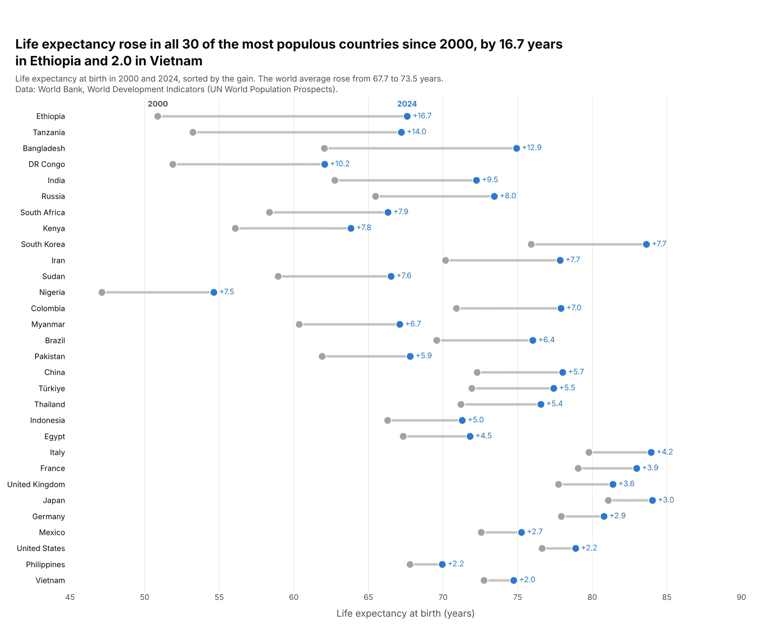
Dumbbell chart of life expectancy in 2000 and 2024 for the 30 most populous countries, sorted by the gain. Ethiopia rose 16.7 years, from 50.9 to 67.6, Tanzania 14.0 and Bangladesh 12.9; Vietnam gained the least, 2.0, and the United States 2.2

Data: World Bank, World Development Indicators (UN World Population Prospects).

How do you read a dumbbell chart? In the example above, notice these things:

Each row is one country, with a gray dot for its life expectancy in 2000, a blue dot for 2024 and a line between them. The gain is printed next to the blue dot, so you don't have to work it out from the axis.
The length of the line is the change, and the rows are sorted by it. That puts Ethiopia's long line, a gain of 16.7 years, at the top and Vietnam's short one at the bottom, so the ranking reads from top to bottom.
Both dots sit on one shared axis, so the chart shows the levels as well as the gaps. Nigeria's row sits far to the left because it had the lowest life expectancy in both years, and Japan's and Italy's rows sit furthest to the right because they had the highest.
Every blue dot is to the right of its gray dot, which means life expectancy rose in all 30 countries. If a value fell, its blue dot would land on the left, so check which end is which color before you read the direction.
The rows are sorted by the gain and not by the level, so a row near the bottom can still have a high life expectancy. The United States gained only 2.2 years, but it started higher than most of the countries above it.

It's often used for charts like these:

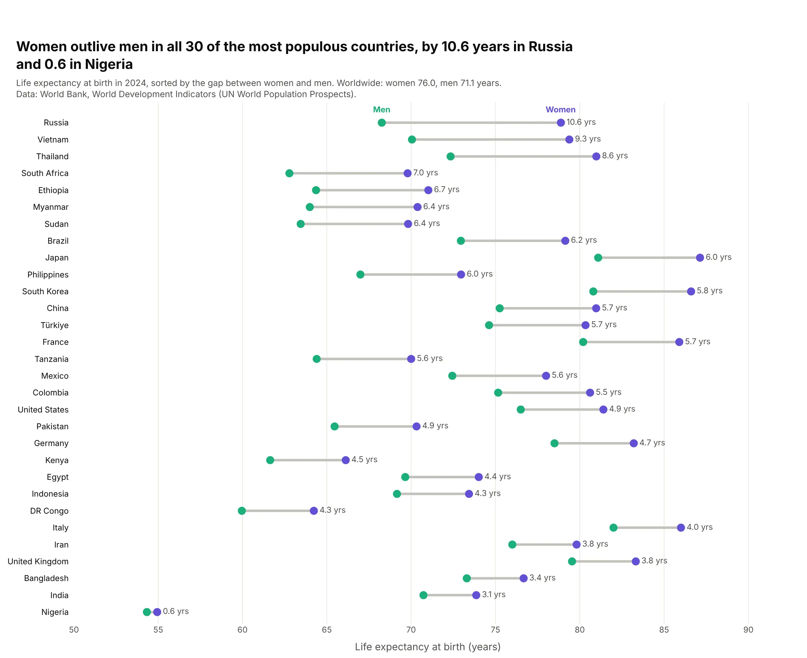
Dumbbell chart of female and male life expectancy in 2024 for the 30 most populous countries, sorted by the gap. Russia has the largest gap, 10.6 years (78.9 vs 68.3), followed by Vietnam (9.3) and Thailand (8.6); Nigeria the smallest at 0.6 years

Two groups instead of two dates. Women outlived men in all 30 of the most populous countries in 2024, by 10.6 years in Russia and 0.6 in Nigeria. Data: World Bank WDI, SP.DYN.LE00.FE.IN and SP.DYN.LE00.MA.IN.

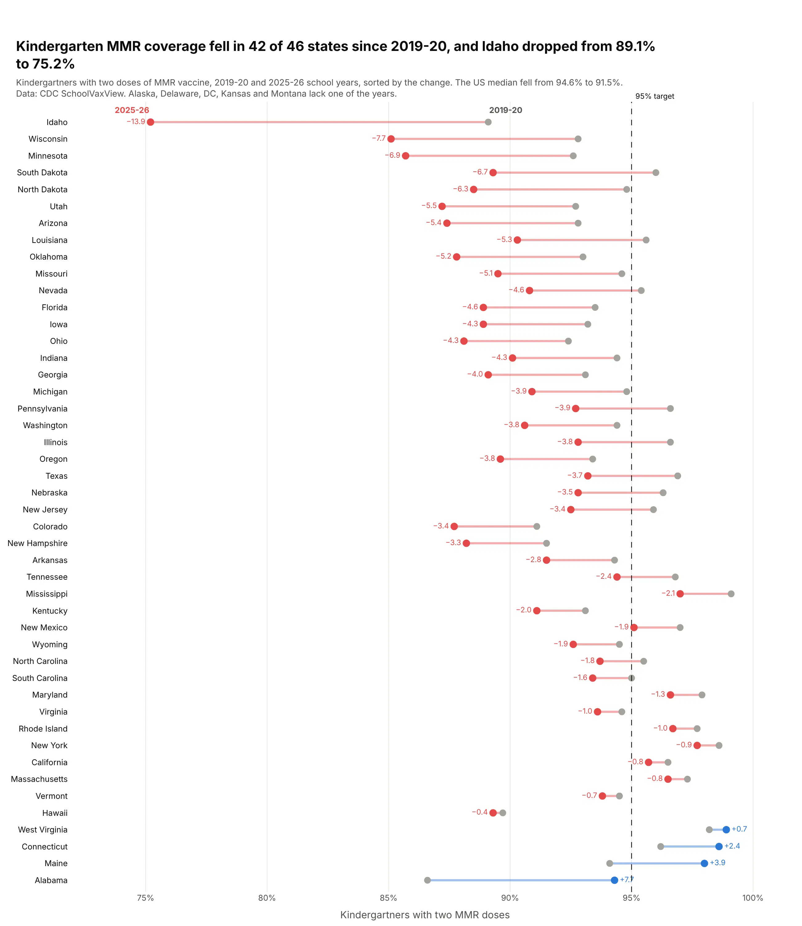
Dumbbell chart of the share of kindergartners with two MMR doses by state in 2019-20 and 2025-26, with a dashed line at the 95% target. Coverage fell in 42 of 46 states, most in Idaho from 89.1% to 75.2%; it rose in Alabama, Maine, Connecticut and West Virginia

A change measured against a target. Two-dose MMR coverage among kindergartners fell in 42 of 46 states between the 2019-20 and 2025-26 school years, and 36 states are now below the 95% target, up from 26. Data: CDC SchoolVaxView (data.cdc.gov, ijqb-a7ye).

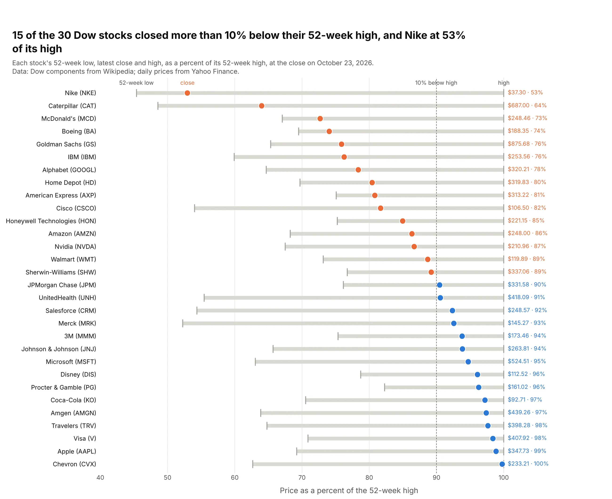
Range chart of the 30 Dow stocks, each drawn from its 52-week low to its high as a percent of the high, with a dot at the October 23, 2026 close. Fifteen closed more than 10% below their high, Nike lowest at 53% ($37.30); Chevron closed at 100% of its high

A range with a third point. On October 23, 2026, 15 of the 30 Dow stocks closed more than 10% below their 52-week high, and Nike closed at 53% of its high. Data: Dow components from Wikipedia; daily prices from Yahoo Finance.

A short history

The dumbbell chart grew out of the dot chart, which William Cleveland proposed in 1984 as a more accurate replacement for bar and pie charts (Cleveland, 1984, The American Statistician), after experiments showed that people judge positions on a common scale better than lengths or areas (Cleveland and McGill, 1984). His best-known dot plots, in the trellis displays he developed at Bell Labs (Becker, Cleveland and Shyu, 1996), put a symbol for each year on every row of the Minnesota barley trials of 1931 and 1932:

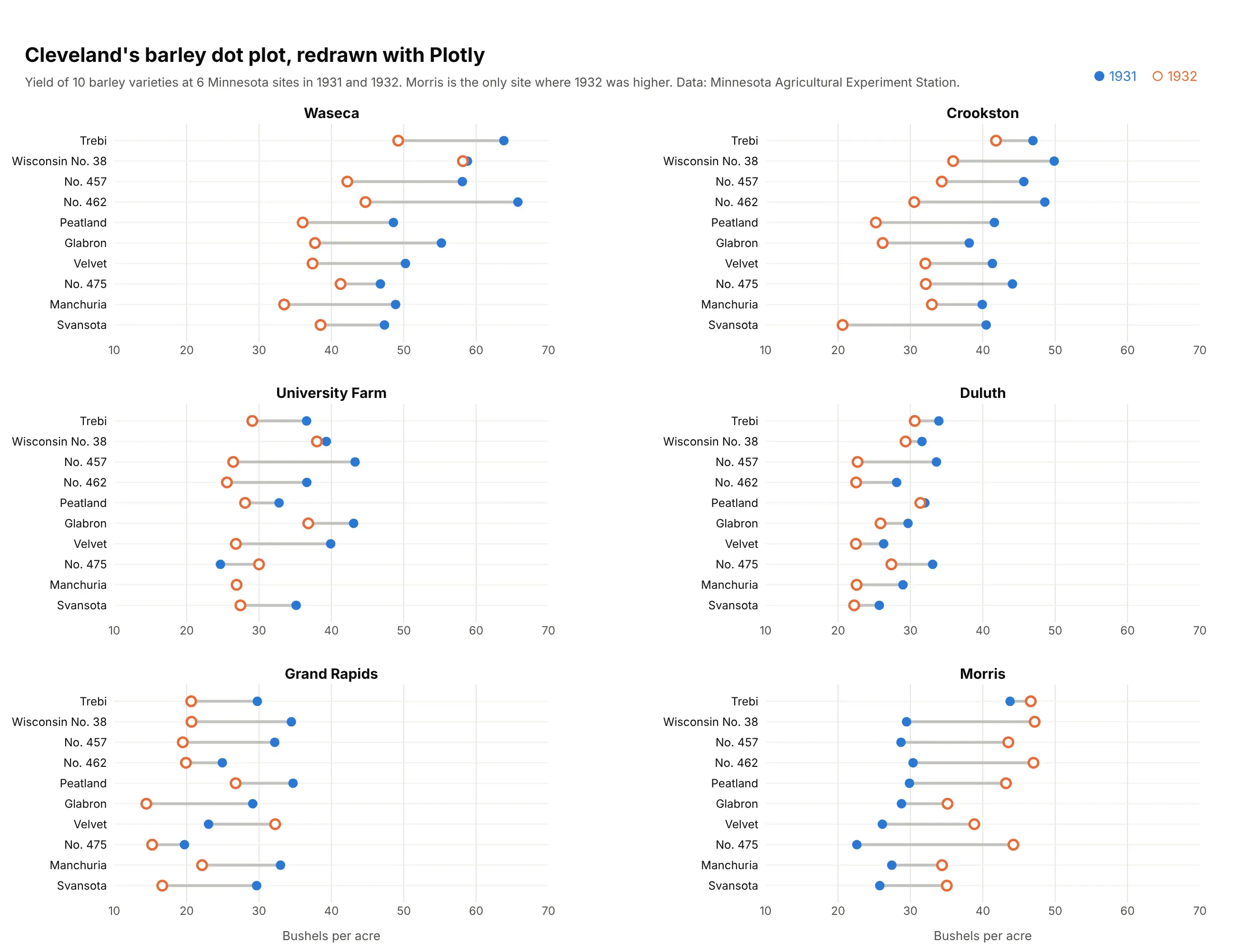
William Cleveland's barley dot plot redrawn with Plotly: yields of 10 barley varieties at 6 Minnesota sites in 1931 (blue dots) and 1932 (orange circles), with a light line joining each pair. At five sites nearly every variety yielded less in 1932, while at Morris all 10 yielded more

Joining the two symbols with a line turns that dot plot into a dumbbell chart, and the line makes the Morris site stand out, because it is the only one where all 10 varieties grew more in 1932. Newspapers and business reports later adopted the style under several names: dumbbell, barbell, connected dot plot and DNA chart.

Alternatives to a dumbbell chart

Here's the same renewable share of electricity in 2015 and 2024 drawn six ways. Some are better for the question, some worse, some just different:

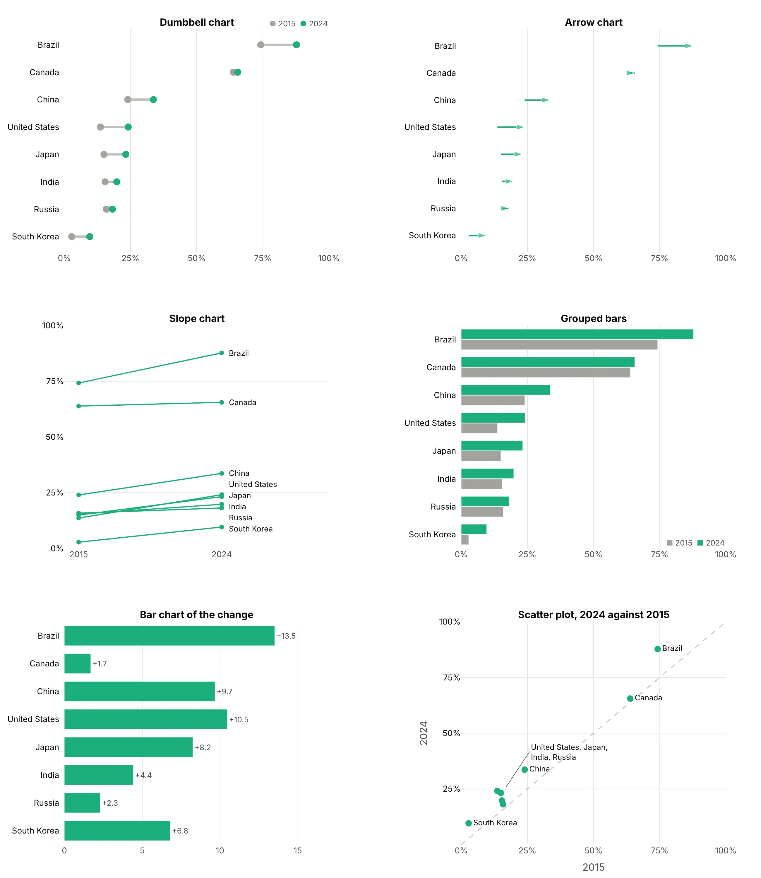
The renewable share of electricity in 2015 and 2024 for the 8 largest electricity generators drawn six ways: a dumbbell chart, an arrow chart, a slope chart, grouped bars, a bar chart of the change (Brazil +13.5 points, Canada +1.7) and a scatter plot of 2024 against 2015 with a dashed no-change line

Arrow chart (works too, when direction matters). The same rows with an arrowhead at the newer value, which shows direction without relying on color. Here every country rose, so the arrows add little, but in data where some rows fall and some rise they read faster than colored dots.
Slope chart (better for a few rows). The two values sit on two vertical axes, so the change becomes an angle. It's very readable up to about 15 lines, and here the four countries that started between 13% and 16% already cross. See our slope chart guide.
Grouped bars (worse for the gap). Each value is a length from zero, which is right when the size relative to zero matters, but the reader has to work out the change from two bars, and 30 rows become a wall of bars.
Bar chart of the change (better for ranking the change). Brazil's 13.5-point gain and Canada's 1.7 are easy to compare, but the levels are gone, so you can't see that Brazil and Canada were already above 60%.
Scatter plot of one value against the other (different). Every point above the diagonal rose. It's the better choice when the two values have different units, but labels crowd where values are close, as for the four countries near 20%.

How to make a dumbbell chart

With AI

ChatGPT, Claude Code, GitHub Copilot, Cursor and other AI tools are excellent at writing Plotly code. Name Plotly in the prompt, describe the two values and the sort, and list the checks you want:

Make a plotly dumbbell chart from prices.csv (columns: state, price_2019, price_2025).

- Draw the connectors as ONE go.Scatter in mode="lines"
  with None between rows, plus one marker trace per year. Don't use add_shape in a loop.
- One row per state, sorted by percent change, biggest at the top.
- Gray 2019 dot, 2025 dot orange if the change beats 25.9% inflation, else blue.
- Print the percent change after each row. Name the years above the top row, no legend.
- A title that states the takeaway with a number, and a muted subtitle with the source.
- Assert there is exactly one row per state and no missing values.
- Save it as dumbbell.html and as a PNG at 2x scale.

With Plotly Studio

Plotly Studio is a desktop app where you point an AI at a dataset and it builds charts and a Dash app around your questions. Ask for a dumbbell chart the same way:

Show a dumbbell chart of residential electricity prices by state in 2019 and 2025, sorted by the percent change. Color the 2025 dot orange where prices rose faster than inflation, print the change after each row, and add a dropdown to switch between residential, commercial and industrial prices.

Make a dumbbell chart in Python or JavaScript

This is the code AI tools write under the hood. In Python, this helper builds a dumbbell chart from three go.Scatter traces, sorts the rows by the change, prints it and names the two ends above the top row:

import pandas as pd
import plotly.graph_objects as go


def make_dumbbell(df, label, start, end, names=("Before", "After"),
                  colors=("#a3a29b", "#2a78d6"), down_color=None):
    d = df.assign(gap=df[end] - df[start]).sort_values("gap")
    xs, ys = [], []
    for a, b, c in zip(d[start], d[end], d[label]):
        xs += [a, b, None]  # None breaks the line between rows
        ys += [c, c, None]
    end_colors = [down_color if down_color and g < 0 else colors[1] for g in d.gap]
    fig = go.Figure([
        go.Scatter(x=xs, y=ys, mode="lines", line=dict(color="#c3c2bc", width=4)),
        go.Scatter(x=d[start], y=d[label], mode="markers", marker=dict(size=12, color=colors[0])),
        go.Scatter(x=d[end], y=d[label], mode="markers+text", marker=dict(size=12, color=end_colors),
                   text=[f"{g:+.1f}" for g in d.gap], textposition="middle right"),
    ])
    top = d.iloc[-1]  # name the two ends above the top row instead of a legend
    for x, text, color in [(top[start], names[0], colors[0]), (top[end], names[1], colors[1])]:
        fig.add_annotation(x=x, y=top[label], yshift=20, text=f"<b>{text}</b>",
                           showarrow=False, font=dict(color=color))
    fig.update_layout(template="simple_white", showlegend=False,
                      yaxis=dict(categoryorder="array", categoryarray=list(d[label])))
    return fig


df = pd.DataFrame({"country": ["Ethiopia", "India", "Japan", "United States"],
                   "le_2000": [50.9, 62.8, 81.1, 76.6], "le_2024": [67.6, 72.2, 84.0, 78.9]})
fig = make_dumbbell(df, "country", "le_2000", "le_2024", names=("2000", "2024"))
fig.show()

In JavaScript, plotly.js builds the same three traces, with null between rows in the connector trace:

<div id="chart"></div>
<script src="https://cdn.plot.ly/plotly-4.1.1.min.js"></script>
<script>
  const rows = [  // sorted by the gain, smallest first (plotly draws the first row at the bottom)
    {country: "United States", y2000: 76.6, y2024: 78.9},
    {country: "Japan", y2000: 81.1, y2024: 84.0},
    {country: "India", y2000: 62.8, y2024: 72.2},
    {country: "Ethiopia", y2000: 50.9, y2024: 67.6},
  ];
  const names = rows.map(r => r.country);
  Plotly.newPlot("chart", [
    {  // every connector in one trace; null breaks the line between rows
      x: rows.flatMap(r => [r.y2000, r.y2024, null]),
      y: rows.flatMap(r => [r.country, r.country, null]),
      mode: "lines", line: {color: "#c3c2bc", width: 4}, hoverinfo: "skip"
    },
    {x: rows.map(r => r.y2000), y: names, mode: "markers", name: "2000",
     marker: {size: 12, color: "#a3a29b"}},
    {x: rows.map(r => r.y2024), y: names, mode: "markers+text", name: "2024",
     marker: {size: 12, color: "#2a78d6"}, textposition: "middle right",
     text: rows.map(r => "+" + (r.y2024 - r.y2000).toFixed(1))}
  ], {showlegend: false, yaxis: {categoryorder: "array", categoryarray: names}});
</script>

Keep the connectors in one trace. Drawing them with fig.add_shape() in a loop works for 20 rows, but in our benchmark 1,000 rows took 186 seconds to build that way and 23 ms as one trace.

Share it

Every Plotly chart has a Share chart button (the cloud icon in its toolbar) that uploads it to Plotly Cloud and gives you a link. Only you can see it until you change its visibility.

For a live app, put the chart in a Dash app and publish it with the Plotly Cloud CLI. Coding agents can run these commands for you:

pip install "dash[cloud]"
plotly user login
plotly app publish

If your data has to stay in your own cloud or data center, publish to Dash Enterprise instead.

Dos and don'ts

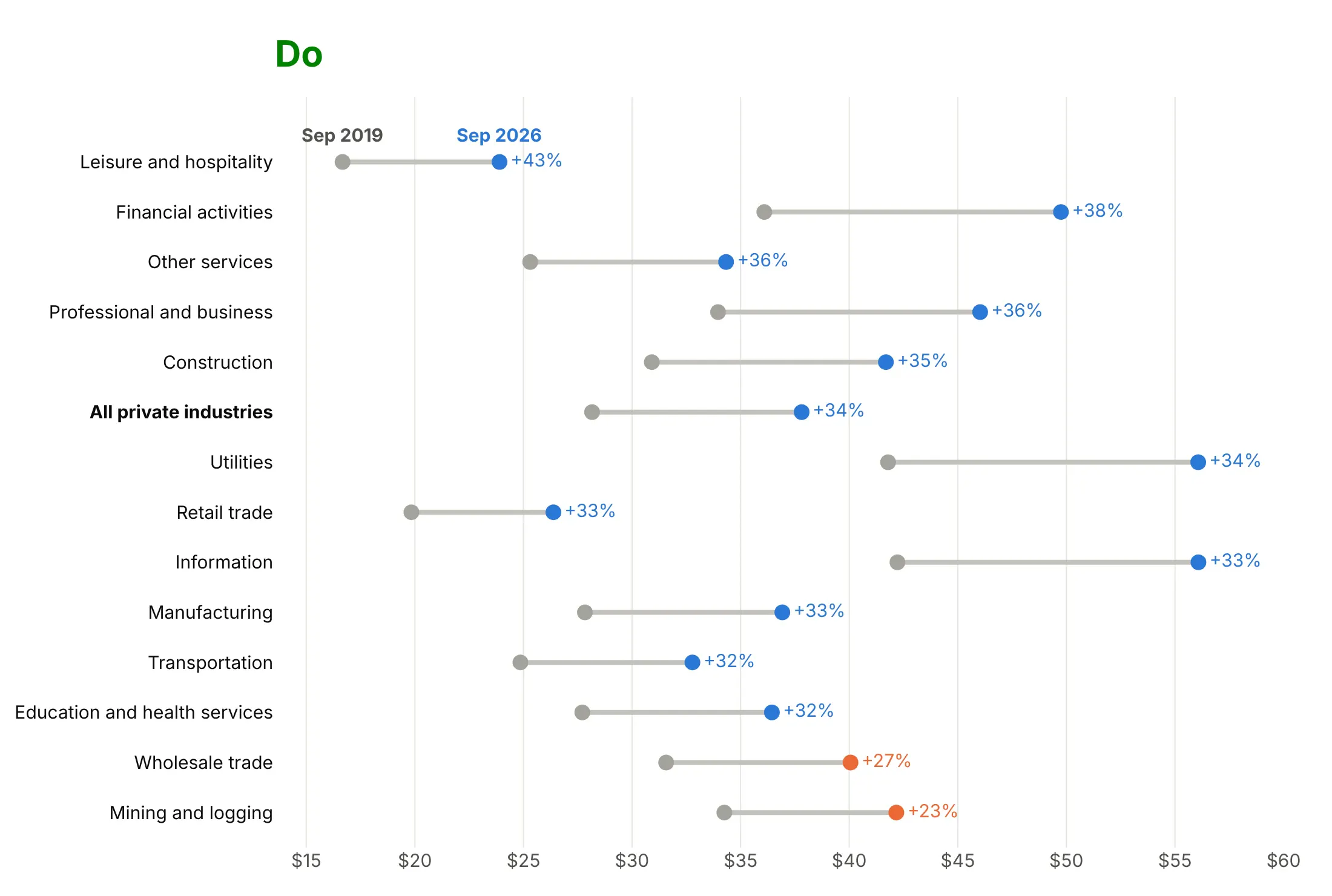
Plotly treats a dumbbell like any scatter plot, so the rows come in the order of your data and the legend shows your trace names. For a published chart, most of the work is sorting, labeling and printing the numbers. Here is the same wage data both ways, average hourly earnings by industry in September 2019 and September 2026.

Don't list the rows alphabetically, force the axis to start at zero, leave raw column names in the legend or the values off the rows. Both charts use the same colors, but here the pattern is hard to find and every change has to be estimated by eye:

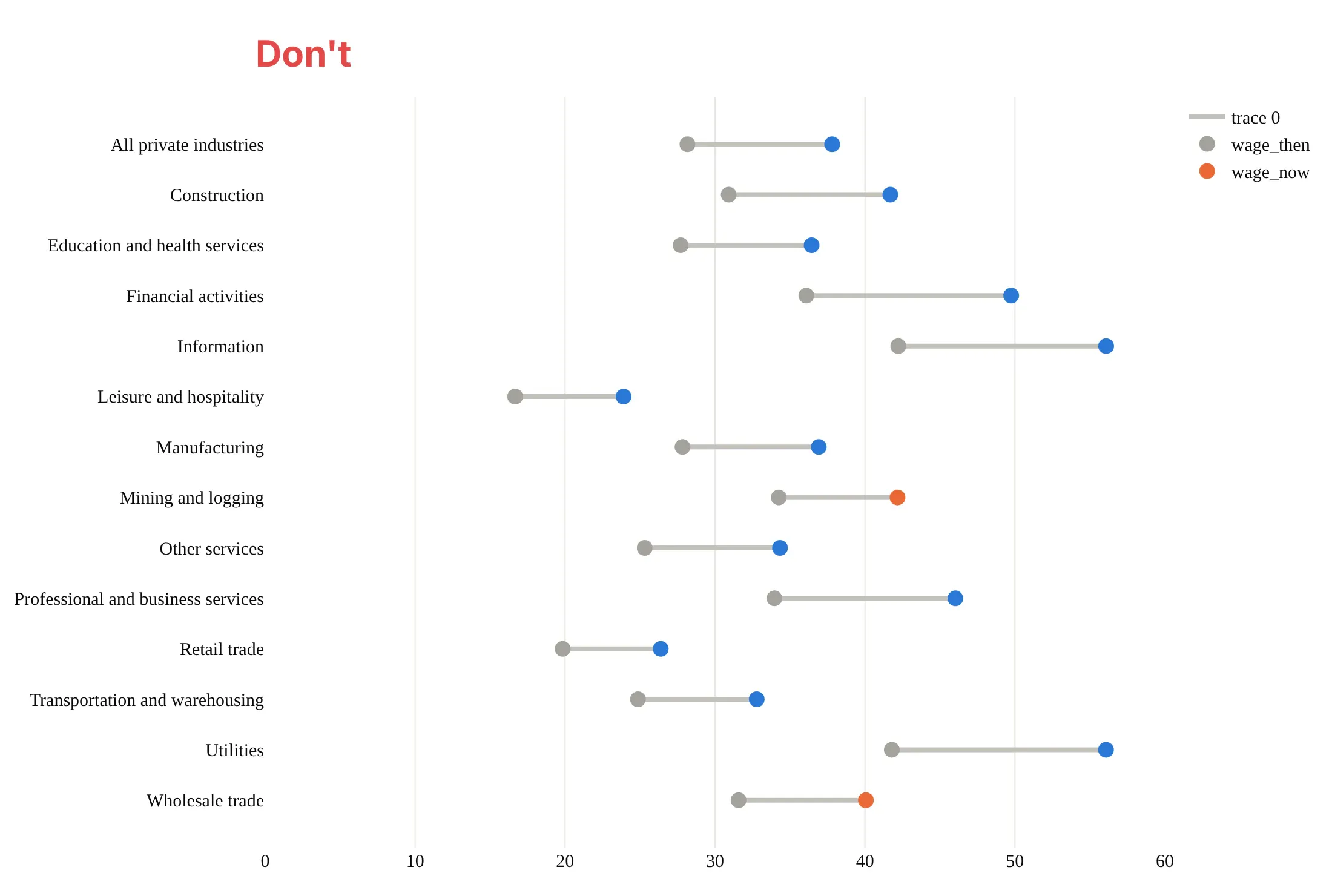
A dumbbell chart of average hourly earnings by industry with the same gray, blue and orange dots as the designed version, but with rows in alphabetical order, an x axis from 0 to 60 without dollar signs that squeezes the gaps, a legend reading trace 0, wage_then and wage_now, no values on the rows and a serif font

Do sort the rows by the change, keep the connector gray, color the newer dot by whether pay beat the 31.1% rise in consumer prices, print the change and name the two dates above the top row:

The same dumbbell chart designed on purpose: rows sorted by the change from leisure and hospitality (+43%) at the top to mining and logging (+23%) at the bottom, gray connectors, blue end dots for industries whose pay beat inflation and orange for wholesale trade and mining and logging, which did not, and Sep 2019 and Sep 2026 labeled above the top row

Use color for one thing

Color decides what a dumbbell chart says. Here are four options on the same data, fossil CO2 per person in 1990 and 2024 for the 10 countries that emit the most.

One color per end. Works when every row moves the same way, but here it hides that half the countries fell and half rose.

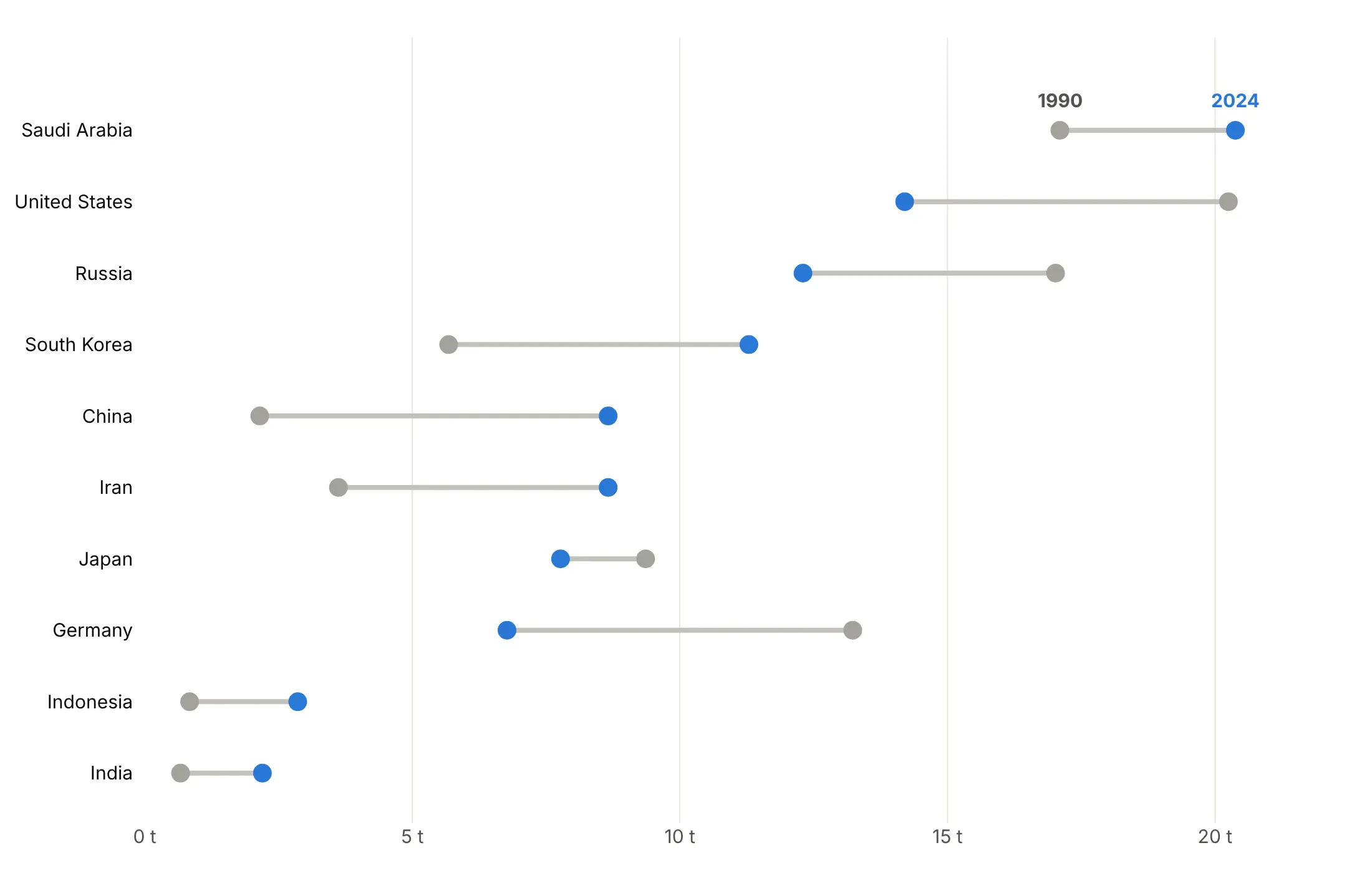
Dumbbell chart of CO2 per person in 1990 and 2024 for the 10 largest emitters, with every 1990 dot gray and every 2024 dot blue

Color by direction. Blue for a fall and orange for a rise shows the split at once: the US, Russia, Japan and Germany fell, and the other six rose.

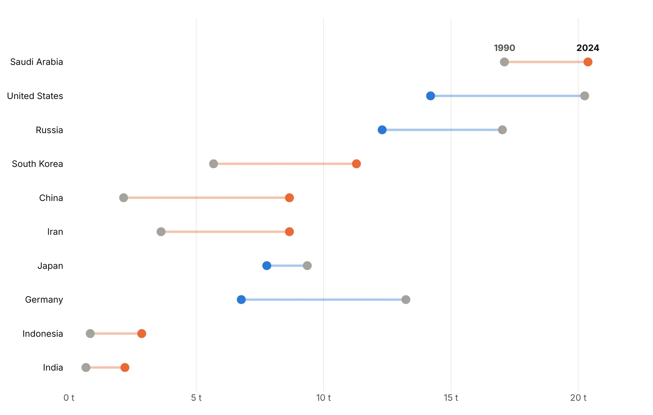
The same dumbbell chart with the United States, Russia, Japan and Germany in blue because their emissions per person fell, and Saudi Arabia, South Korea, China, Iran, Indonesia and India in orange because theirs rose

Arrows. The direction is in the shape, so it survives grayscale printing and color blindness.

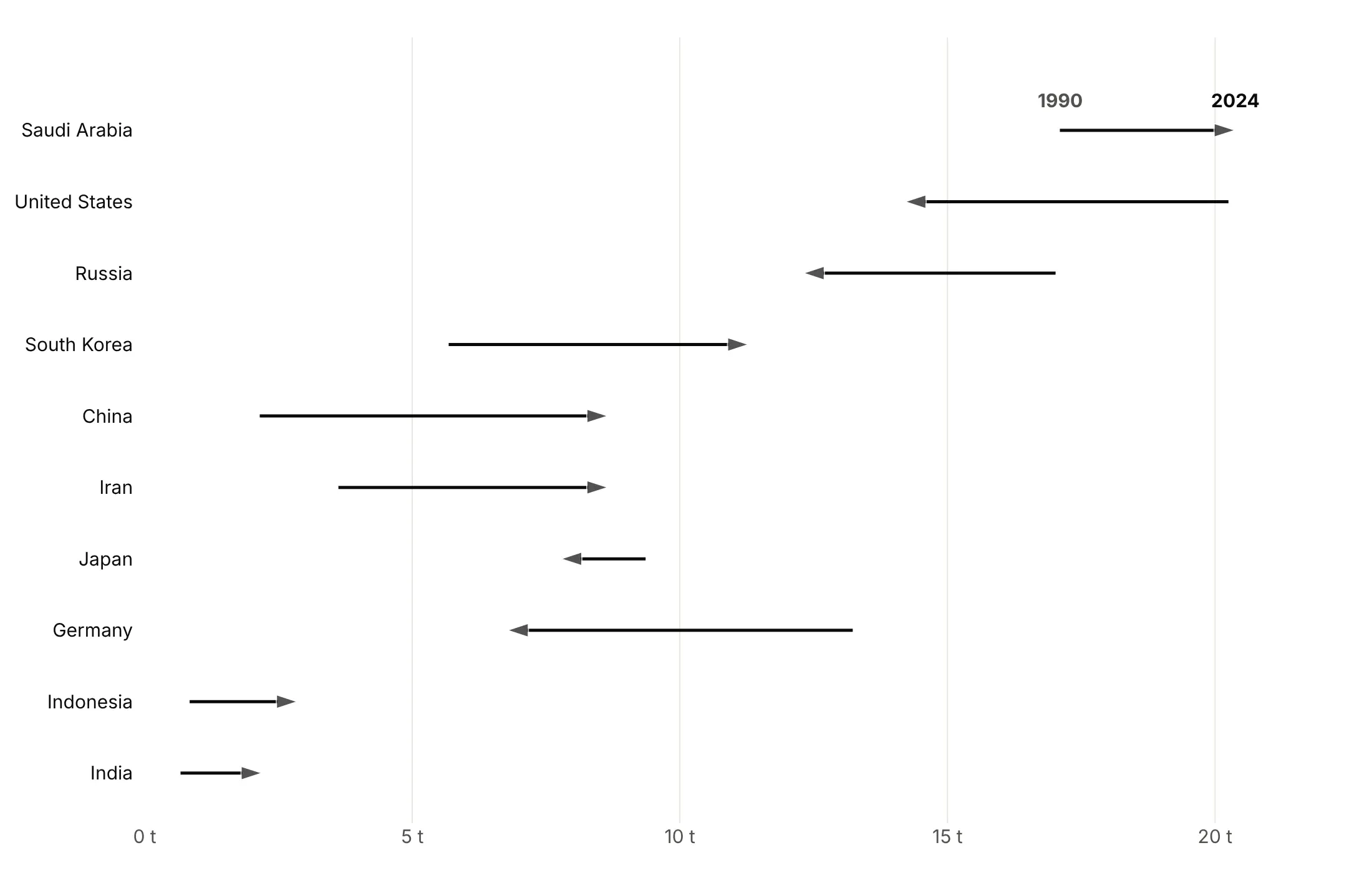
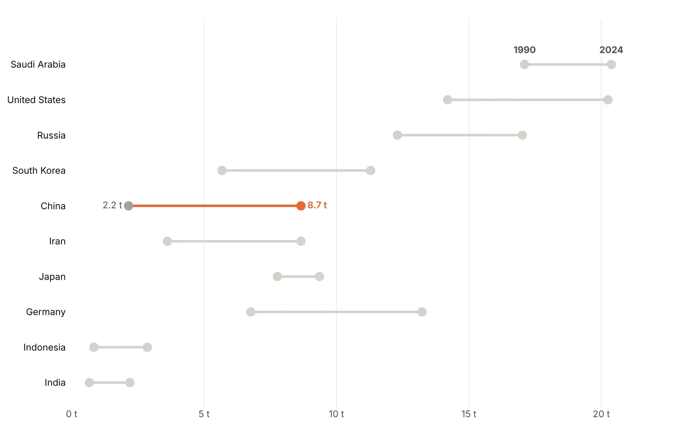
Highlight one row. When the text is about one country, make everything else gray. China went from 2.2 to 8.7 tonnes per person.

The same dumbbell chart in light gray except China, drawn in orange from 2.2 tonnes in 1990 to 8.7 tonnes in 2024

Checklist

Sort the rows by the gap, or by the end value when levels matter more.
Name the two ends above the top row instead of using a legend.
Print the change at the end of each row, so nobody has to subtract.
Color by meaning: direction, above or below a benchmark, or one highlighted row.
Add a reference line for a target, parity or the overall rate (95% vaccination, 50% women, .500).
Use a log axis when values span orders of magnitude, so equal percentage changes get equal lengths.

Don't

Start the axis at zero by default, because a dumbbell shows positions, not lengths.
Put two different units on one axis; use a scatter plot instead.
Leave raw column names such as wage_now in a legend; name the two ends on the chart instead.
Draw the connectors with fig.add_shape() in a loop.

Options to customize

A dumbbell chart is built from go.Scatter traces and a few layout settings. These are the ones that matter most; the full list is in the Plotly scatter reference.

go.Scatter(mode="lines") with None in x and y: one trace draws every connector, and None breaks the line between rows. Always use it; it's the fast way.
go.Scatter(mode="markers"): one trace per end (start, end, or a median for ranges).
mode="markers+text", text, textposition: prints values next to a dot; textposition can be a list, so falls print on the left.
marker.color as a list: one color per row, for direction or a benchmark.
marker.symbol="arrow" with marker.angleref="previous": arrowheads that point along the connector, for an arrow chart in one trace.
fig.add_annotation(ax=..., axref="x", showarrow=True): an arrow from one value to another with full control, for up to a few hundred rows.
yaxis.categoryorder="array" and categoryarray: fixes the row order, so you can sort by the gap.
xaxis.type="log": for values that span orders of magnitude.
fig.add_vline, fig.add_vrect: a reference line or band for a target, parity or a benchmark range.
fig.add_annotation(yshift=20, showarrow=False): a label above the top row that names the two ends.
make_subplots(rows=1, cols=2): two side-by-side columns for more than about 40 rows.
fig.update_layout(shapes=[...]): sets many shapes at once if you need shapes; never add_shape in a loop.
hovertemplate, customdata: put the other value or the change in the hover text.

More dumbbell chart examples

Ten more dumbbell charts built from real public data, each with its source, the technique that makes it work and a prompt to rebuild it.

1. What Medicare pays per prescription for its top drugs

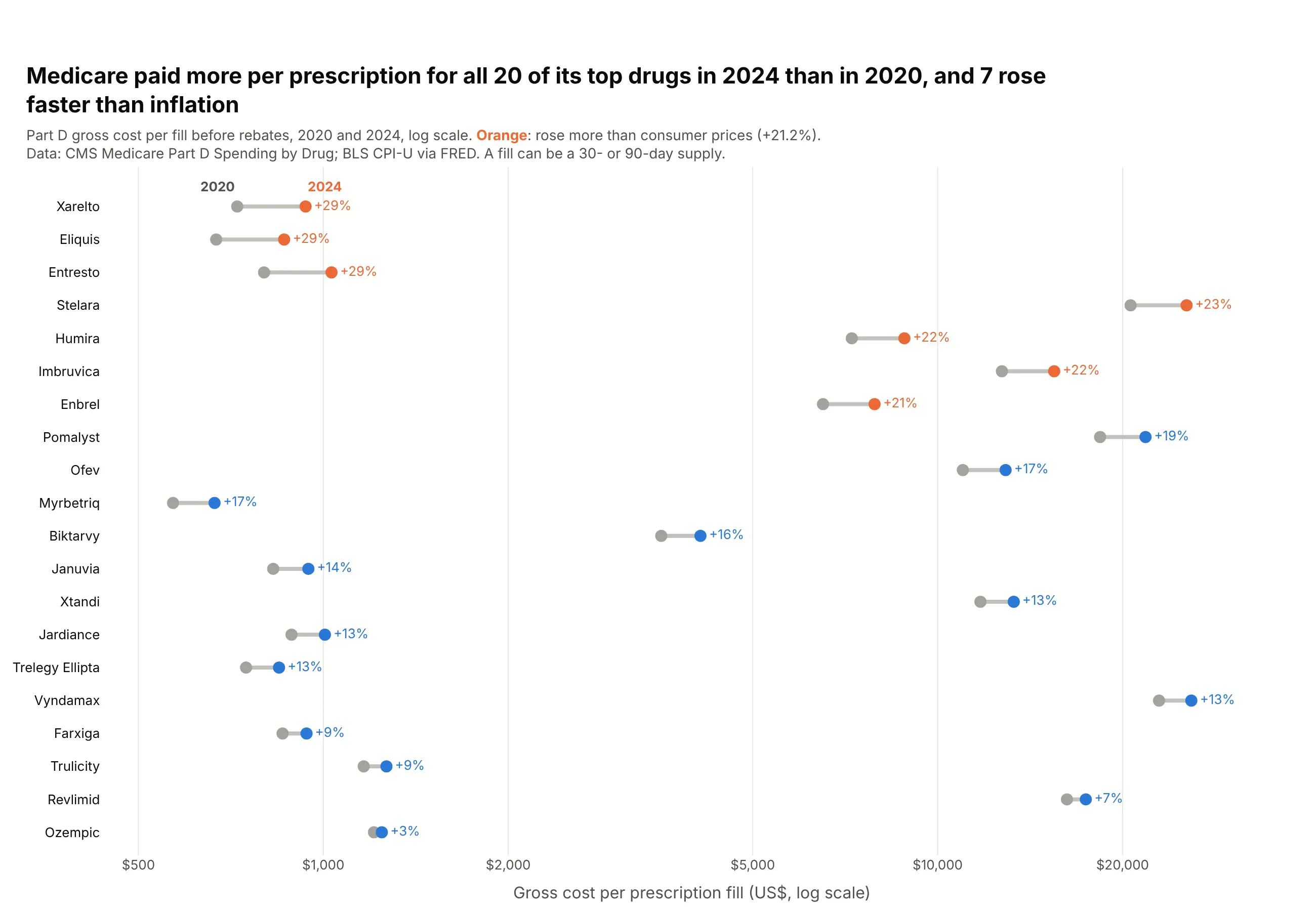
Dumbbell chart on a log scale of Medicare Part D gross cost per prescription fill in 2020 and 2024 for the 20 drugs with the most spending. All rose; Xarelto, Eliquis and Entresto rose 29% and are orange for beating 21.2% inflation, and Ozempic rose 3%

Medicare Part D paid more per prescription fill in 2024 than in 2020 for all 20 of its top-selling drugs. Seven rose faster than consumer prices (21.2%), led by Xarelto (+29%) and Eliquis, which went from $669 to $863 per fill. Data: CMS Medicare Part D Spending by Drug, gross cost before rebates.

Tip: a log x axis lets a $665 drug and a $25,882 drug share one chart, and equal percentage rises get equal lengths.

Get the data from CMS "Medicare Part D Spending by Drug" (data.cms.gov), the "Overall" row per
brand, columns Avg_Spnd_Per_Clm_2020 and Avg_Spnd_Per_Clm_2024, plus CPI-U (FRED CPIAUCSL)
annual averages for 2020 and 2024
and shape it into a table (columns: brand, generic, spend_2024_bn, per_fill_2020, per_fill_2024, change_pct).
Keep the 20 brands with the highest 2024 spending that have 2020 data.

Build a plotly dumbbell chart on a log x axis, sorted by change_pct.
- 2024 dot orange if the rise beats CPI, else blue; print "+29%" after each row.
- Subtitle: gross cost before rebates; a fill can be 30 or 90 days.

2. How long Phase 3 trials take, by therapeutic area

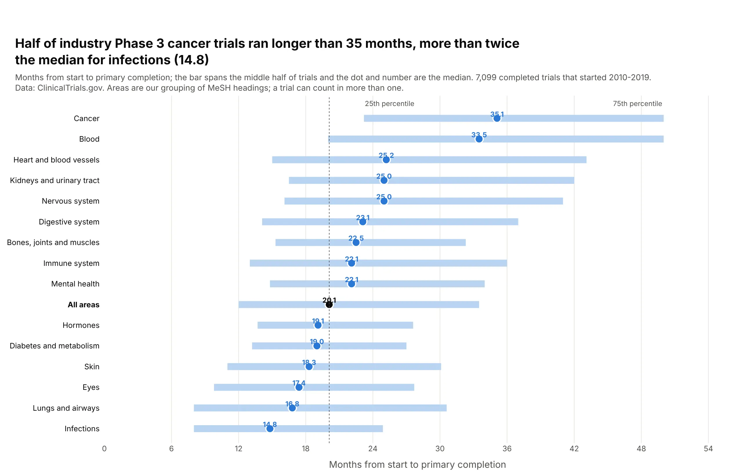
Range chart of months from start to primary completion for 7,099 completed industry Phase 3 trials started 2010-2019, with a bar for the middle half and a dot for the median. Cancer trials have the longest median at 35.1 months (23.2 to 50.0), infections the shortest at 14.8; the all-areas median is 20.1

Half of the industry-funded Phase 3 cancer trials that started in 2010-2019 took longer than 35.1 months to reach primary completion, 2.4 times the median for infections (14.8). Across 7,099 trials the median was 20.1 months. Data: ClinicalTrials.gov API v2 (areas are our grouping of MeSH headings).

Tip: a range is a dumbbell with a third point: draw the 25th to 75th percentile as a thick light line and the median as a dot on top.

Get the data from the ClinicalTrials.gov API v2: completed interventional Phase 3 studies with an
industry lead sponsor that started 2010-2019, with start date, primary completion date and condition
MeSH terms and ancestors
and shape it into a table (columns: area, trials, p25_months, median_months, p75_months).
Map trials to ~15 areas by top-level MeSH heading; a trial can count in several.

Build a plotly range chart: thick light-blue line from p25 to p75, blue median dot, sorted by median.
- Median value printed above each dot; "All areas" row in black with a dotted reference line.

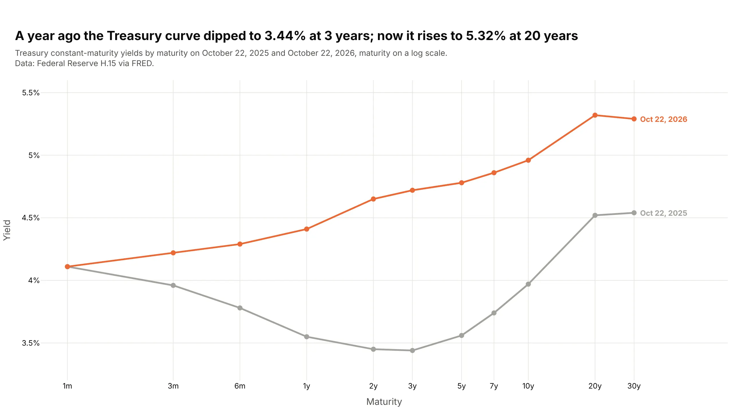
3. How the Treasury yield curve moved in a year

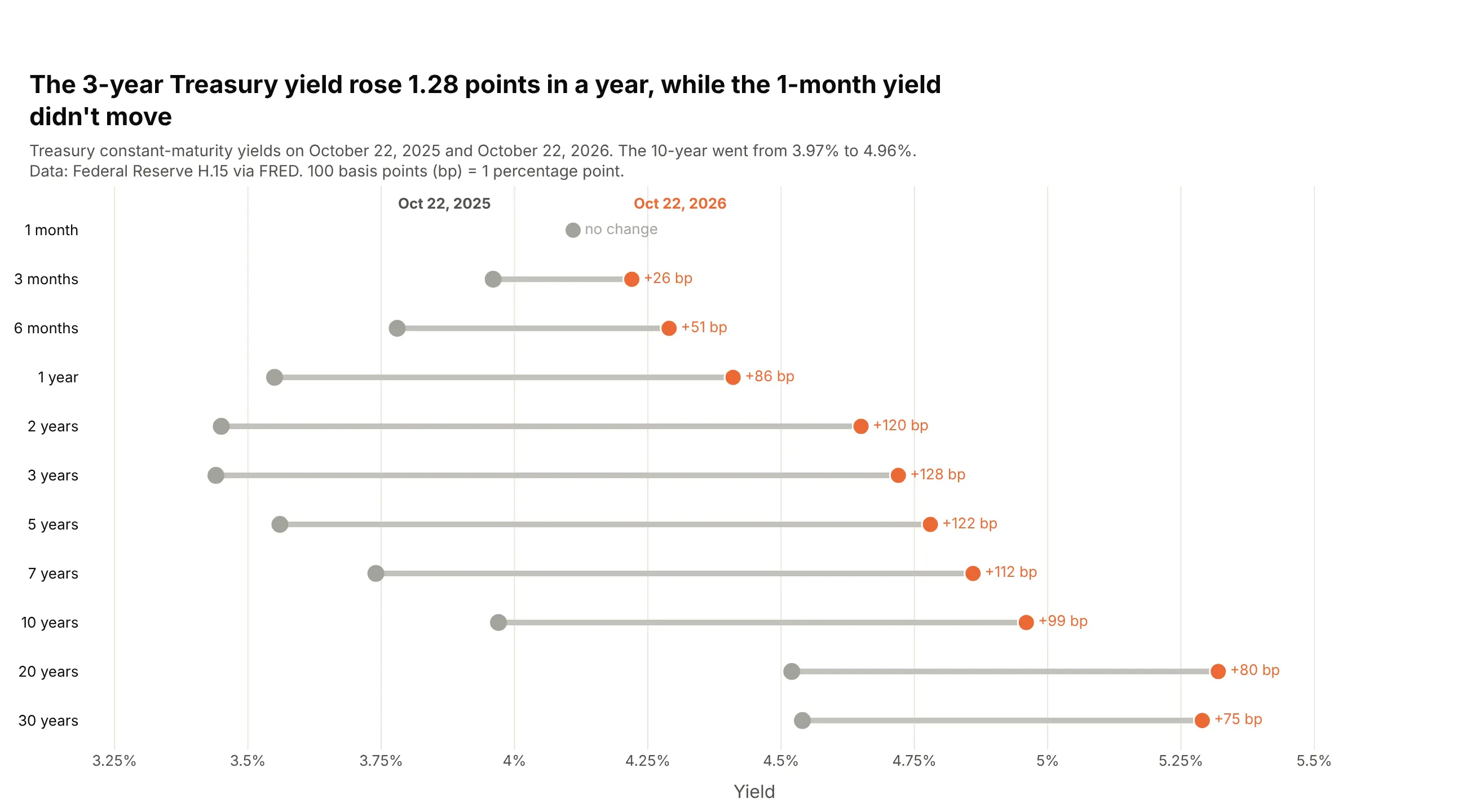
Dumbbell chart of Treasury yields at 11 maturities on October 22, 2025 and October 22, 2026. Every maturity except 1 month rose: the 3-year yield by 128 basis points (3.44% to 4.72%), the 2-year by 120 and the 10-year by 99 to 4.96%; the 1-month stayed at 4.11%

From October 2025 to October 2026 the 3-year Treasury yield rose 1.28 points, from 3.44% to 4.72%, while the 1-month yield stayed at 4.11%. The 10-year went from 3.97% to 4.96%. Data: Federal Reserve H.15 via FRED.

Tip: keep the maturities in their natural order instead of sorting by change, because the order carries meaning.

Get the data from FRED's daily Treasury constant-maturity yields (DGS1MO, DGS3MO, DGS6MO, DGS1, DGS2,
DGS3, DGS5, DGS7, DGS10, DGS20, DGS30) on the latest common date and one year earlier
and shape it into a table (columns: maturity, years, yield_then, yield_now, change_bp).

Build a plotly dumbbell chart with maturities top to bottom from 1 month to 30 years.
- Gray dot for a year ago, orange for now; "+128 bp" after each row, "no change" in gray.

Another way to see it: the usual yield curve line chart shows the curve's shape, a dip to 3.44% at 3 years a year ago, but the size of each move is harder to read than in the dumbbell.

Line chart of the Treasury yield curve on October 22, 2025, dipping from 4.11% at 1 month to 3.44% at 3 years, and on October 22, 2026, rising from 4.11% to 5.32% at 20 years

4. Residential electricity prices by state

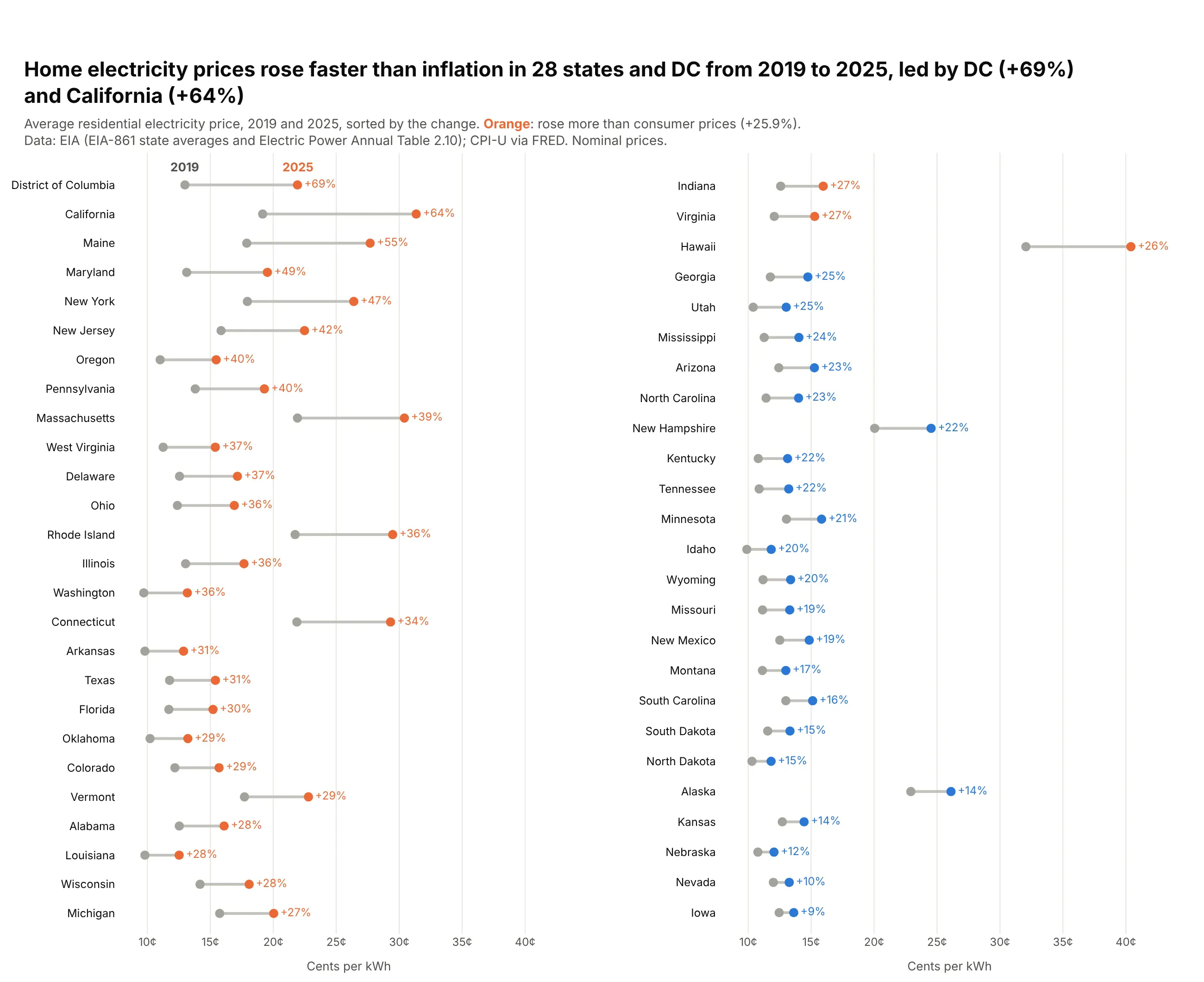
Two-column dumbbell chart of average residential electricity prices in 2019 and 2025 for 50 states and DC, sorted by the change. DC rose 69% and California 64% to 31.35 cents; 28 states and DC rose more than 25.9% inflation and are orange; Iowa rose least at 9%

Home electricity prices rose faster than inflation (25.9%) in 28 states and DC between 2019 and 2025, and no state's price fell. California's rose 64% to 31.35 cents per kWh. Data: EIA (EIA-861 state averages and Electric Power Annual, Table 2.10).

Tip: split 51 rows into two side-by-side columns with make_subplots(rows=1, cols=2), sorted top-left to bottom-right.

Get the data from EIA's "Average Price by State by Provider" (avgprice_annual.xlsx, 2019, Total Electric
Industry) and the Electric Power Annual Table 2.10 (2025), residential, plus CPI-U annual averages
and shape it into a table (columns: state, code, price_2019, price_2025, change_pct).

Build a plotly dumbbell chart in two columns (make_subplots), sorted by change_pct.
- 2025 dot orange if the change beats CPI, else blue; print "+64%" after each row.

5. CO2 per person since 1990, with arrows

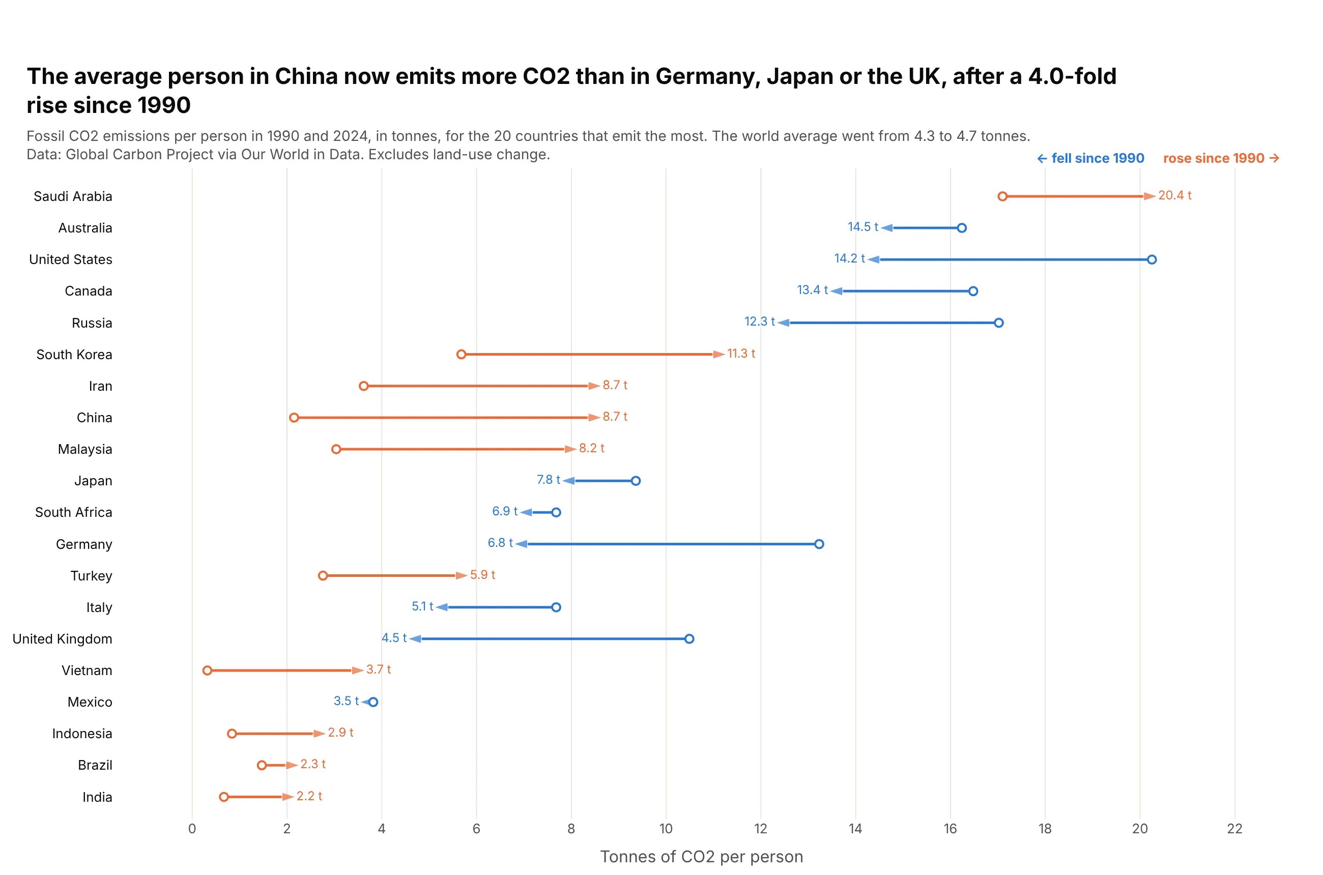
Arrow chart of fossil CO2 per person in 1990 and 2024 for the 20 largest emitters. China rose from 2.2 to 8.7 tonnes, now above Japan (7.8), Germany (6.8) and the UK (4.5); the UK fell 57% and the US from 20.3 to 14.2

The average person in China emitted 8.7 tonnes of fossil CO2 in 2024, 4.0 times as much as in 1990 and more than in Japan, Germany or the UK. Ten of the 20 largest emitters fell and ten rose. Data: Global Carbon Project via Our World in Data.

Tip: use marker.symbol="arrow" with marker.angleref="previous" on the connector trace so each row ends in an arrowhead.

Get the data from Our World in Data's CO2 dataset (owid-co2-data.csv), co2 and co2_per_capita, 1990 and 2024
and shape it into a table (columns: country, co2_mt_latest, per_capita_1990, per_capita_latest, change_pct).
Keep the 20 largest emitters in 2024.

Build a plotly arrow chart: one lines+markers trace per direction with None gaps,
marker symbols ["circle", "arrow", ...] and angleref="previous"; blue for a fall, orange for a rise.
- Sort by 2024 value; print "8.7 t" at the arrowhead.

6. US oil production by state

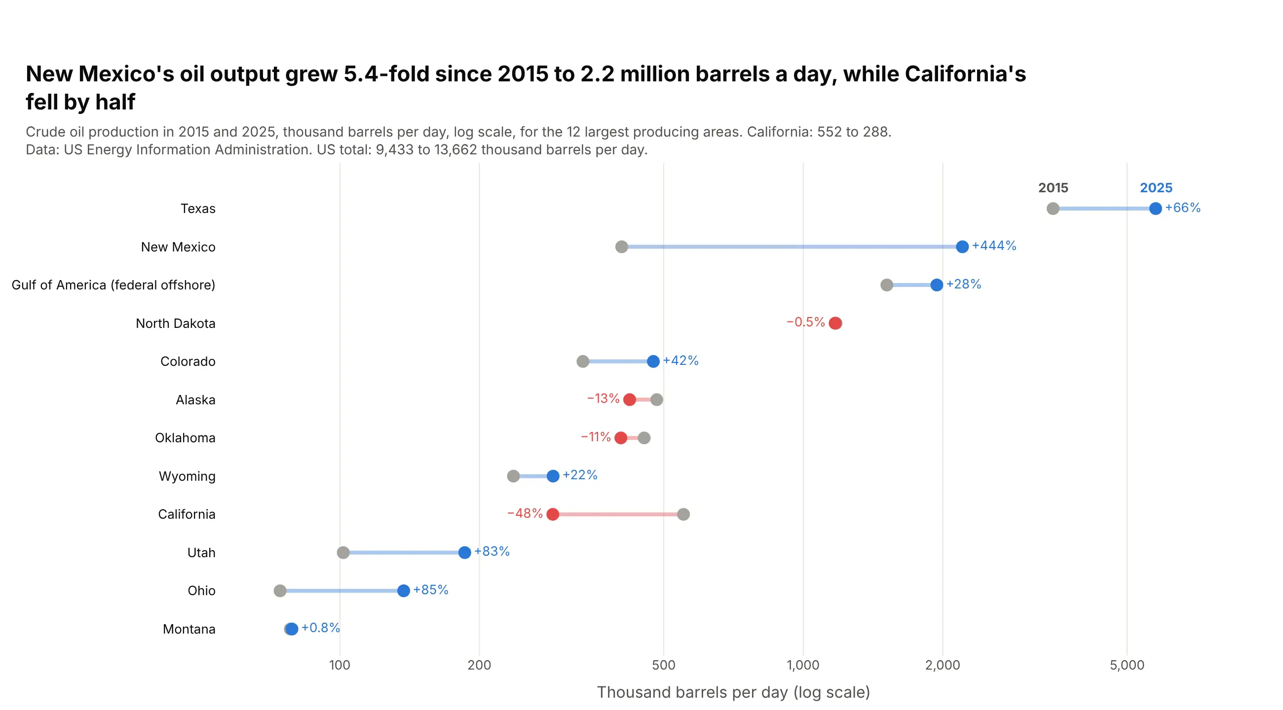
Dumbbell chart on a log scale of crude oil production in 2015 and 2025 for the 12 largest US producing areas. New Mexico grew 443% to 2,205 thousand barrels a day and Texas 66% to 5,761; California fell 48% to 288 and Alaska 13%

New Mexico produced 2.2 million barrels of oil a day in 2025, 5.4 times its 2015 output, while California's production fell by half. US output rose from 9.4 to 13.7 million barrels a day. Data: EIA, Crude Oil Production by state.

Tip: when one row (Texas, 5.8 million) is 70 times another (Montana), a log axis keeps every row's change visible.

Get the data from EIA's annual "Crude Oil Production" by state (PET_CRD_CRPDN_ADC_MBBL_A.xls), 2015 and 2025,
converted from thousand barrels to thousand barrels per day
and shape it into a table (columns: area, kbd_2015, kbd_2025, change_pct). Keep the 12 largest in 2025.

Build a plotly dumbbell chart on a log x axis, sorted by 2025 output.
- Blue for growth, red for decline; print the percent change on the outer side of the 2025 dot.

7. The gender pay gap in the 25 largest occupations

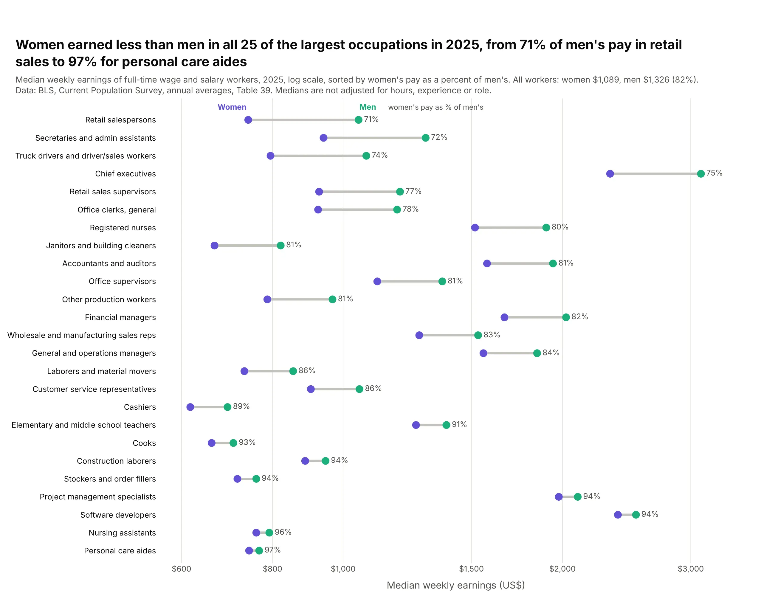
Dumbbell chart on a log scale of median weekly earnings of women and men in the 25 largest occupations in 2025, sorted by women's pay as a percent of men's. Retail salespersons are at 71% ($741 vs $1,050), chief executives 75%, registered nurses 80%, and personal care aides 97%

Women working full time earned less than men in all 25 of the largest occupations in 2025, from 71% of men's median pay among retail salespersons to 97% among personal care aides. Across all workers the figure was 82% ($1,089 vs $1,326). Data: BLS, Current Population Survey, Table 39.

Tip: sort by the ratio, not the dollar gap, and a log axis makes equal ratios equal lengths at any pay level.

Get the data from BLS Current Population Survey Table 39 (cpsaat39.xlsx), median weekly earnings of
full-time workers by detailed occupation and sex, 2025
and shape it into a table (columns: occupation, workers_k, men, women, women_pct_of_men).
Keep the 25 largest detailed occupations with both medians.

Build a plotly dumbbell chart on a log x axis, sorted by women_pct_of_men (lowest at top).
- Women purple, men green; print "71%" after each row.

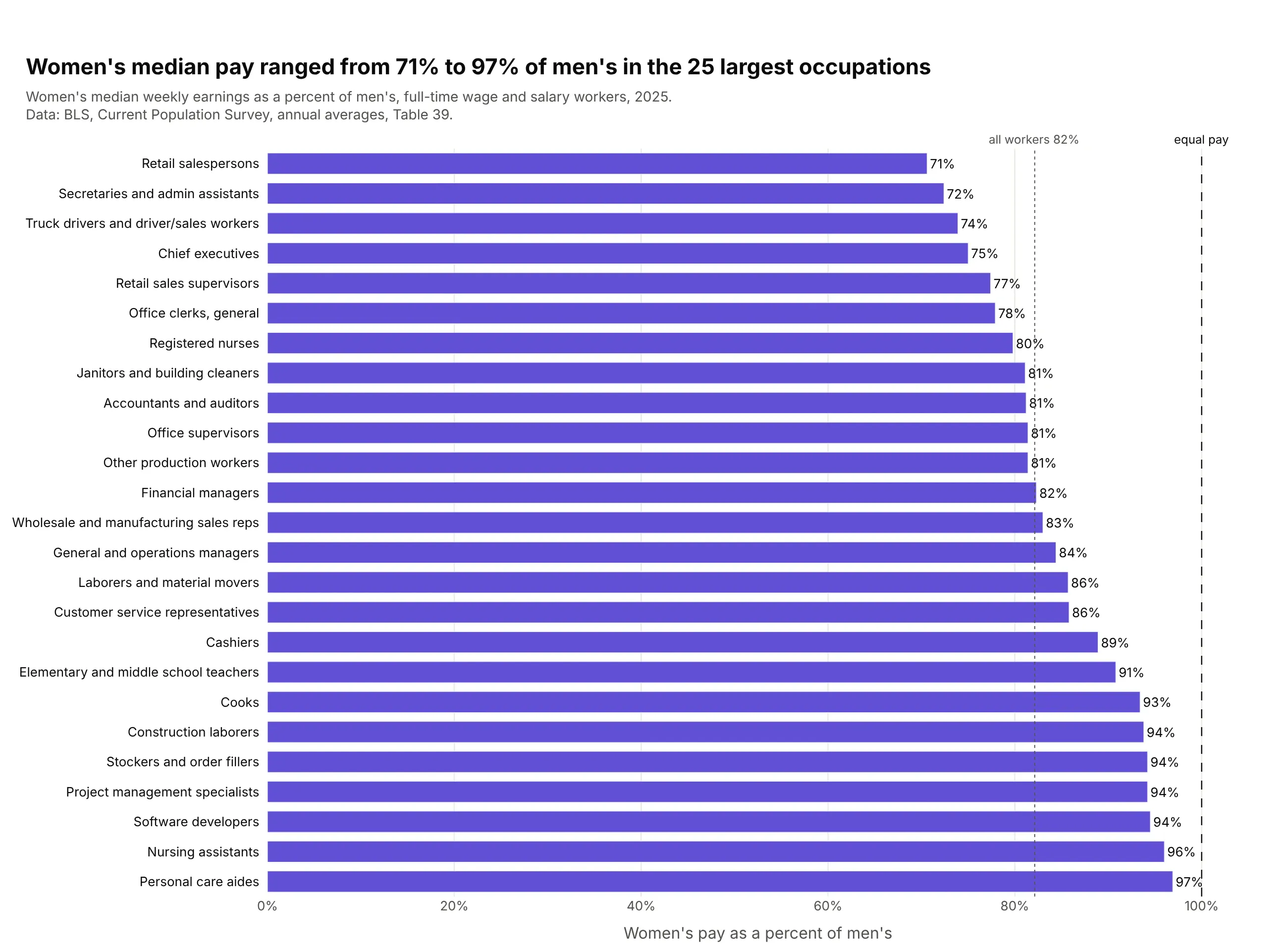
Another way to see it: a bar chart of women's pay as a percent of men's makes the ratio exact, but it drops the pay levels, so chief executives and cashiers look alike.

Bar chart of women's median weekly earnings as a percent of men's in the 25 largest occupations in 2025, from 71% for retail salespersons to 97% for personal care aides, with lines at 82% for all workers and 100% for equal pay

8. Every state swung Republican from 2020 to 2024

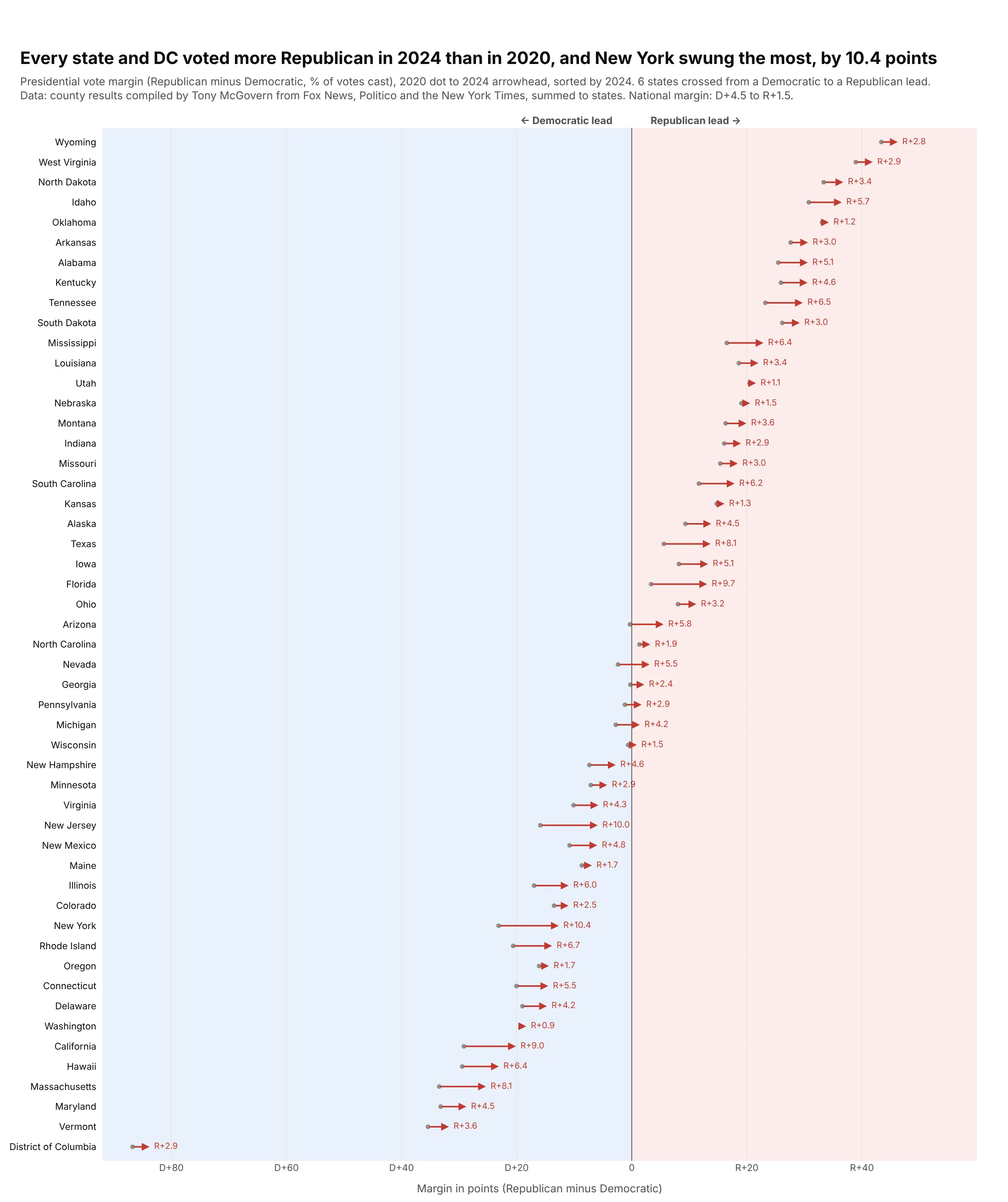
Arrow chart of the Republican-minus-Democratic presidential margin in 2020 and 2024 for 50 states and DC, sorted by the 2024 margin. Every arrow points right; New York swung most, by 10.4 points, and Washington least, 0.9; six states crossed from a Democratic to a Republican lead

Every state and DC voted more Republican in 2024 than in 2020. New York swung the most, 10.4 points, and six states crossed from a Democratic to a Republican lead. Nationally the margin went from D+4.5 to R+1.5. Data: county results compiled by Tony McGovern, summed to states.

Tip: draw each row as fig.add_annotation(x=end, ax=start, axref="x", showarrow=True) when the order in time matters.

Get the data from Tony McGovern's county-level presidential results on GitHub
(tonmcg/US_County_Level_Election_Results_08-24), 2020 and 2024, summed to states
and shape it into a table (columns: state, margin_2020, margin_2024, swing, votes_2024),
margin = (R - D) / total votes x 100.

Build a plotly arrow chart: one annotation arrow per state from the 2020 to the 2024 margin,
sorted by 2024 margin; shade x<0 light blue and x>0 light red; print "R+10.4" after each arrow.

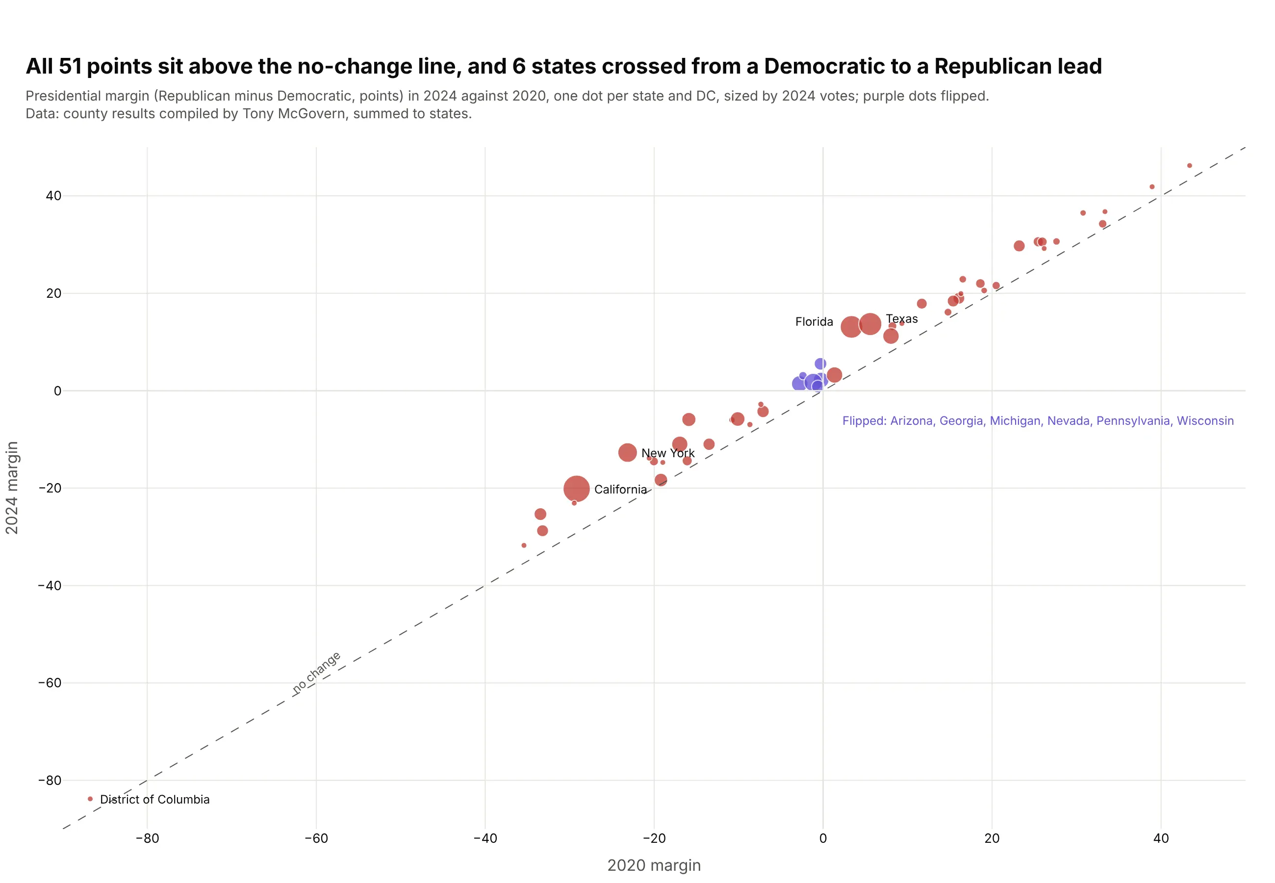
Another way to see it: a scatter of the 2024 margin against the 2020 margin shows every state above the no-change line, but the swing states overlap near zero.

Scatter of 2024 presidential margin against 2020 margin for 51 states and DC, sized by votes, with all points above the diagonal no-change line and six purple flipped states near zero: Arizona, Georgia, Michigan, Nevada, Pennsylvania and Wisconsin

9. Home-field advantage in Major League Baseball

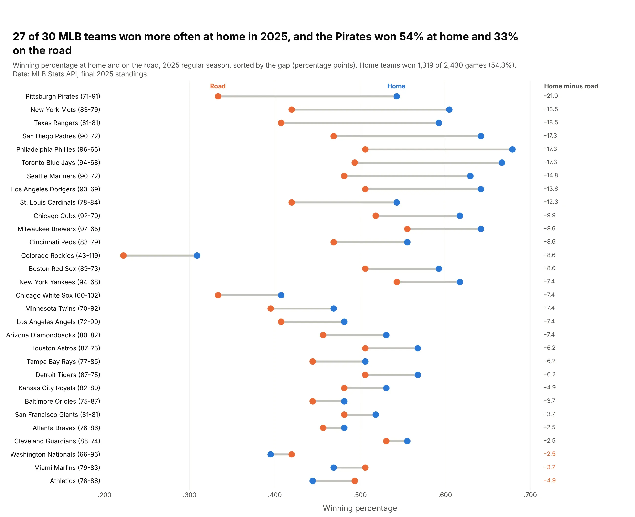
Dumbbell chart of 2025 winning percentage at home and on the road for the 30 MLB teams, sorted by the gap. The Pirates won .543 at home and .333 on the road (21 points); 27 teams did better at home and the Athletics, Marlins and Nationals did better on the road

In 2025, 27 of 30 MLB teams won more often at home, and home teams won 54.3% of all games. The Pirates won 54% at home and 33% on the road. Data: MLB Stats API, final 2025 standings.

Tip: put each team's record in its label and a dashed line at .500, so every row carries its context.

Get the data from the MLB Stats API standings endpoint (statsapi.mlb.com, 2025 regular season)
with home and away split records
and shape it into a table (columns: team, wins, losses, home_w, home_l, away_w, away_l, home_pct, away_pct, gap_pts).

Build a plotly dumbbell chart, road dot orange and home dot blue, sorted by gap_pts;
label rows "Pittsburgh Pirates (71-91)", dashed line at .500, gap printed in a column on the right.

10. Programming languages developers want to use

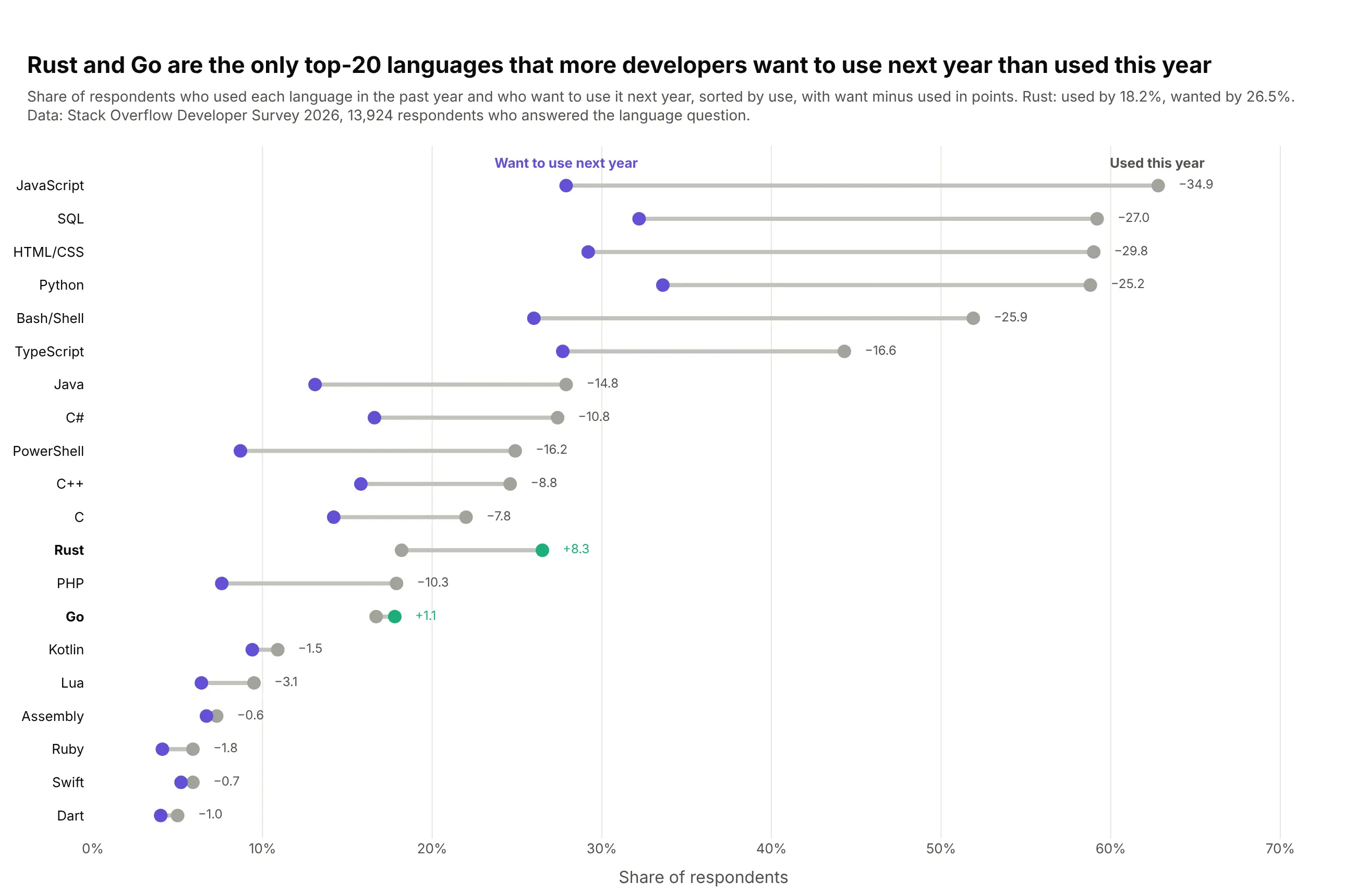
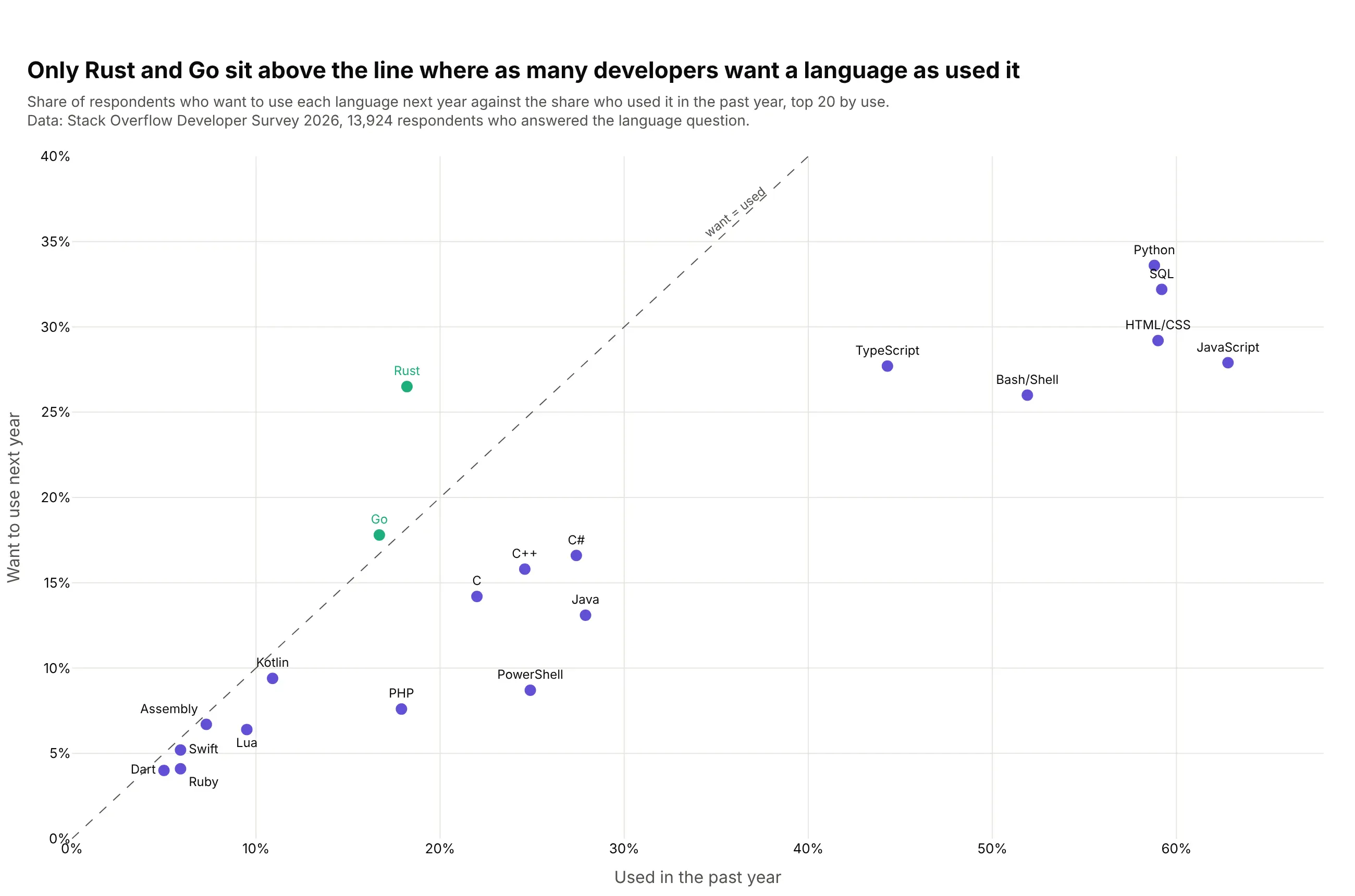
Dumbbell chart of the share of Stack Overflow survey respondents who used each of the top 20 languages in the past year and who want to use it next year. Rust (18.2% used, 26.5% wanted) and Go are the only ones where want exceeds use; JavaScript is used by 62.8% and wanted by 27.9%

Rust and Go are the only top-20 languages that more developers want to use next year than used this year: Rust went from 18.2% of respondents using it to 26.5% wanting it. JavaScript drops from 62.8% to 27.9%. Data: Stack Overflow Developer Survey 2026, 13,924 respondents.

Tip: highlight the exception (want above use) in its own color and bold its row label.

Get the data from the Stack Overflow Developer Survey 2026 public results (survey_results_public.csv),
columns LanguagesHaveWorkedWith and LanguagesWantToWorkWith (semicolon-separated)
and shape it into a table (columns: language, used_pct, want_pct, respondents).
Keep the 20 most used languages, dropping "Other".

Build a plotly dumbbell chart sorted by used_pct; gray "used" dot, purple "want" dot,
green and bold where want exceeds used; print want minus used after each row.

Another way to see it: a scatter of want against used with a diagonal puts Rust and Go above the line, but the ten smallest languages crowd the bottom-left corner.