Chris Parmer

November 3, 2026

Area Charts - A Complete Guide

TL;DR

An area chart is a line chart with the space under the line filled in. A stacked area chart piles several of them on top of each other, so the top edge is the total and each band is one part of it; a 100% stacked area chart rescales every point to 100% to show shares.
Area charts are also known as area graphs, and as layered, step-area or spline-area charts depending on how they're drawn, and are similar to line charts, streamgraphs and small multiples.
Use a stacked area chart when the parts of a total change over time and the total matters too: an energy or electricity mix, population by age group, market share, debt by type. Use overlapping (unstacked) areas to compare two or three series or for categories that overlap, and a line chart when exact values matter.
You can make a Plotly area chart in one line of code in Python with px.area, which stacks the series in one stackgroup; groupnorm="percent" turns it into a 100% stacked area chart. In JavaScript or React, the same chart is plotly.js scatter traces with a shared stackgroup.
See 12 ways to draw an area chart below, from a single filled area and 100% stacked shares to positive and negative fills, range bands, step areas and small multiples, all on 25 years of monthly US electricity data.

What is an area chart?

Stacked area charts look like this:

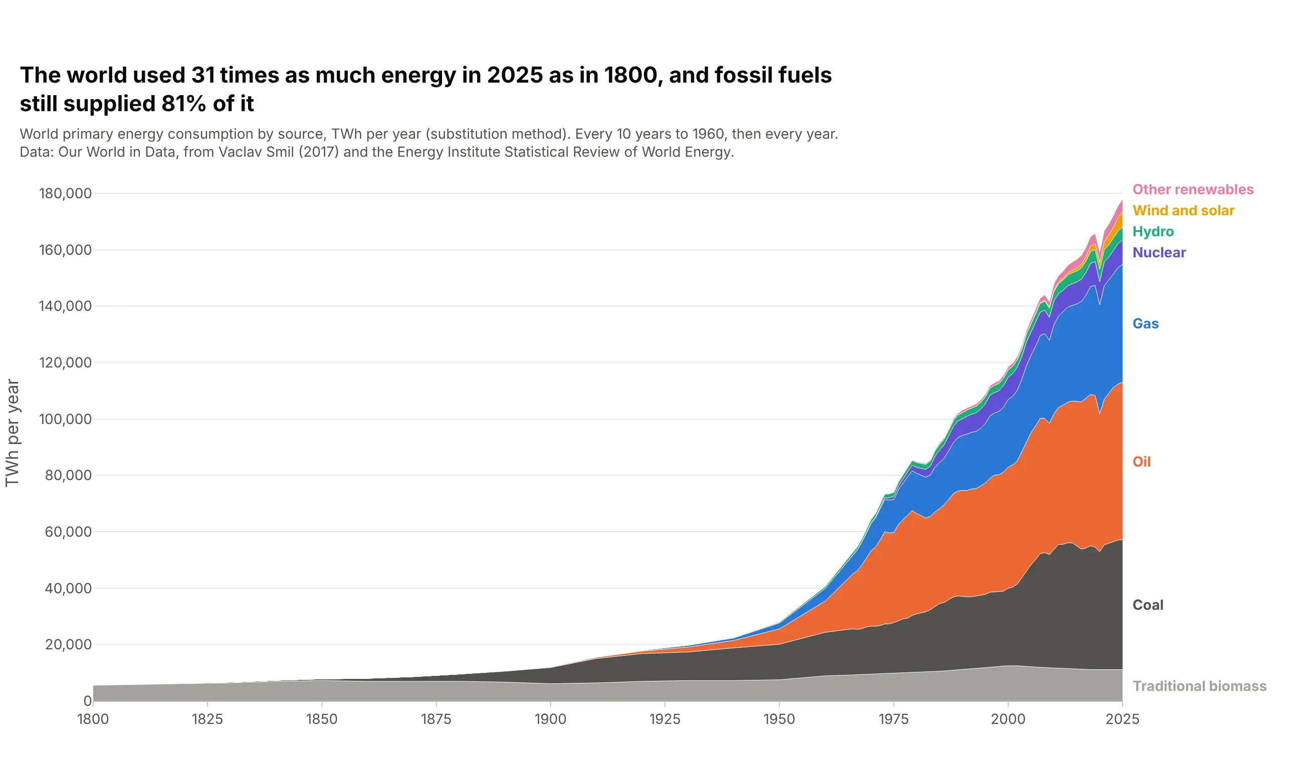
Stacked area chart of world primary energy consumption by source from 1800 to 2025. Traditional biomass is a thin gray band at the bottom, coal grows from 1850, oil from 1910 and gas from 1950, with thin nuclear, hydro, wind and solar and other renewable bands on top; the total rises from 5,653 TWh in 1800 to 177,865 TWh in 2025, 81% of it from fossil fuels

Data: Our World in Data, from Vaclav Smil (2017) and the Energy Institute Statistical Review of World Energy.

How do you read a stacked area chart? In the example above, notice these things:

Each colored band is one source of energy, and its thickness in a year is how much the world used of it. The orange oil band is the thickest in 2025, at 55,826 TWh or 31% of the total.
The top edge is the total, because the bands sit on top of each other. It rises from 5,653 TWh in 1800 to 177,865 TWh in 2025, 31 times as much.
The bands are stacked in the order the fuels arrived, so the chart reads as a history. Traditional biomass was 98% of the total in 1800, and coal passed it between 1900 and 1910.
Only the bottom band sits on a flat baseline. Every other band rides on the bands below it, so judge it by its thickness, not by the height of its top edge. Wind and solar together are the thin yellow band near the top, 3.1% of the total in 2025.

It's often used for charts like these:

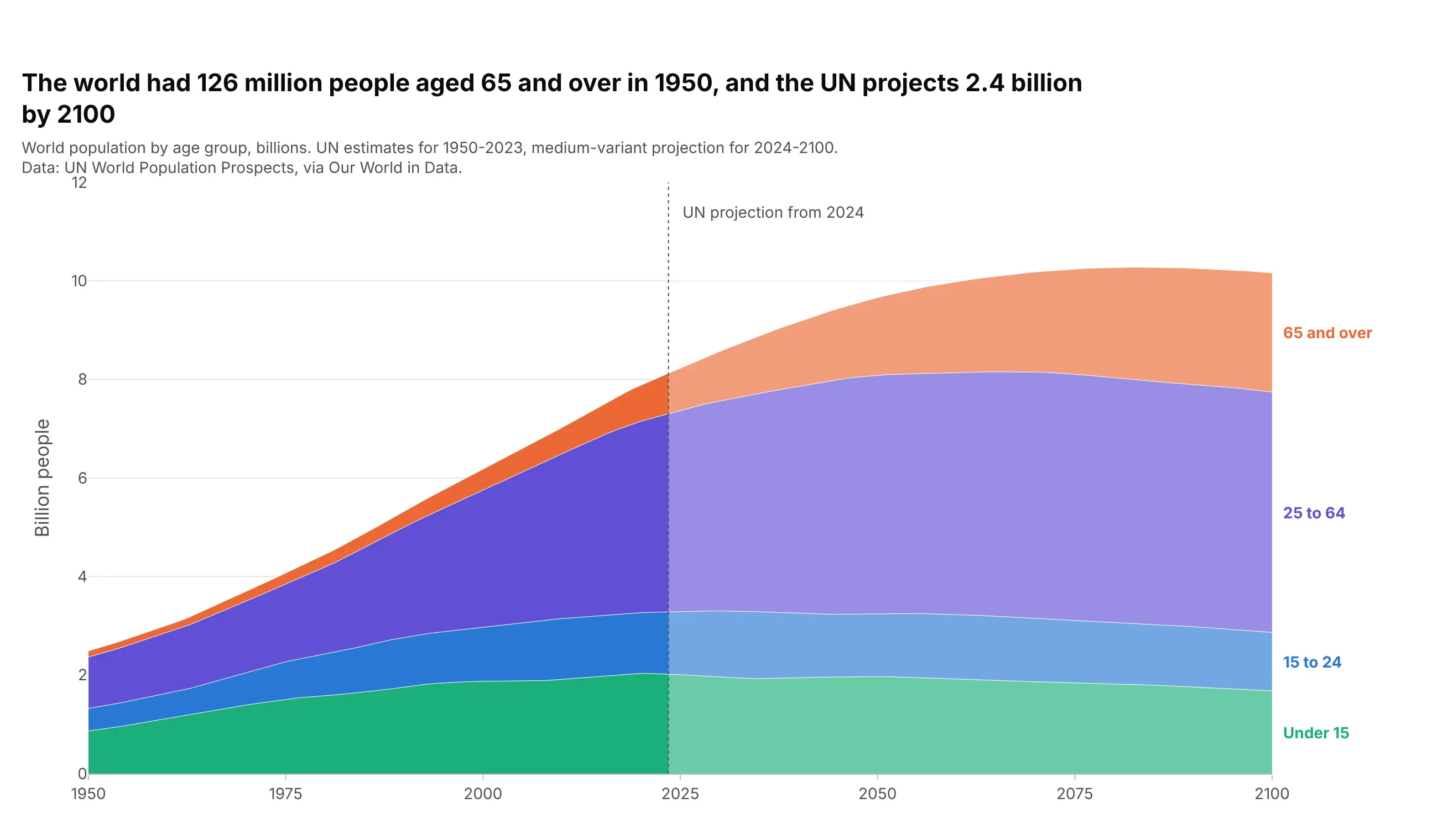
Stacked area chart of world population by age group from 1950 to 2100, with UN projections from 2024 shaded lighter. The 25 to 64 band grows the most, the under 15 band levels off around 2 billion, and the 65 and over band on top grows from 126 million in 1950 to 2.4 billion in 2100

Population by age group. The UN projects 2.4 billion people aged 65 and over in 2100, up from 126 million in 1950, and more of them than children under 15 from 2063. Data: UN World Population Prospects, via Our World in Data.

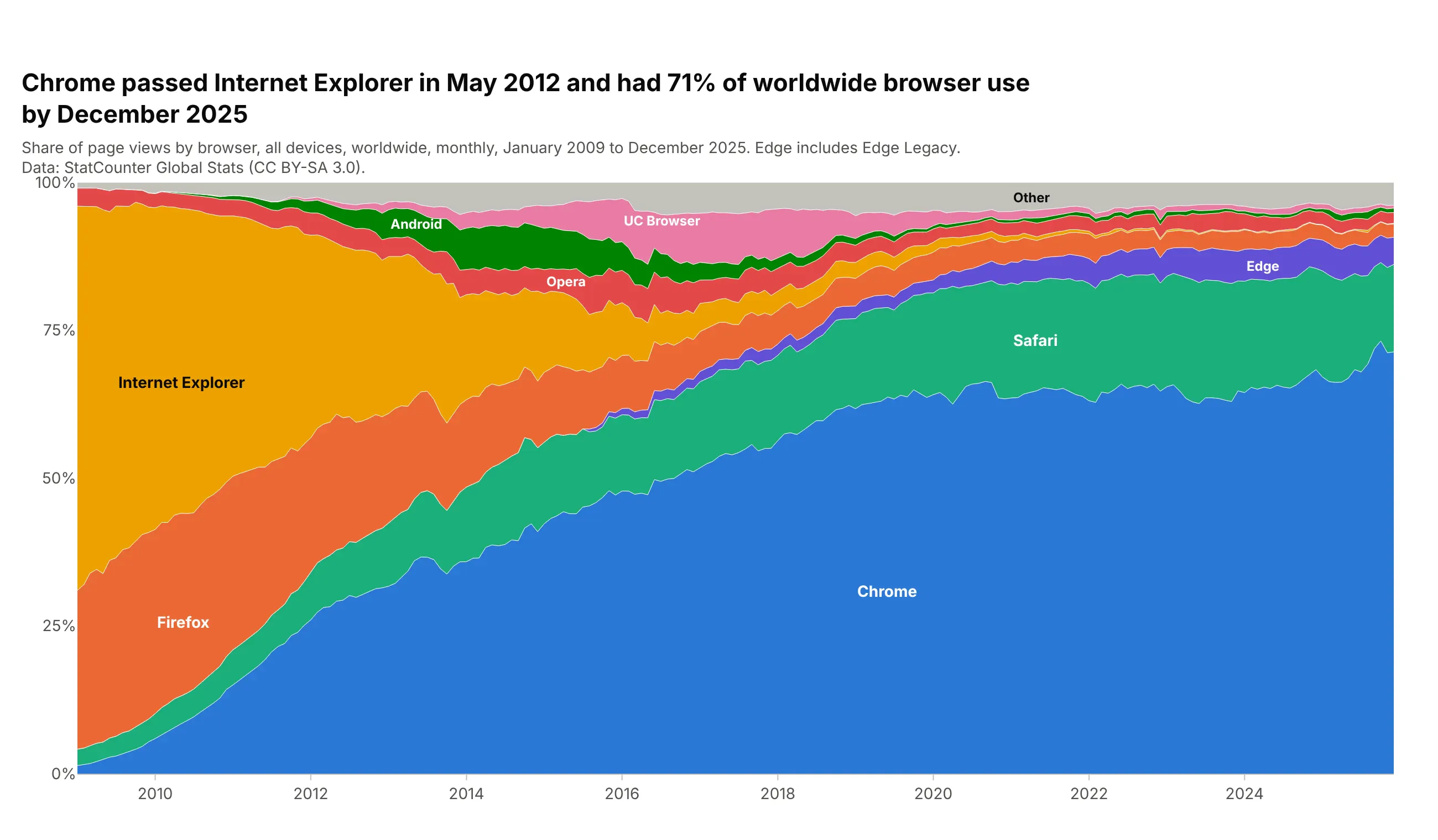
100% stacked area chart of worldwide browser market share by month from 2009 to 2025. Internet Explorer's yellow band shrinks from 65% to almost nothing, Firefox's orange band from 27% fades, and Chrome's blue band at the bottom grows to 71% by December 2025, with Safari above it

Market share over time. Chrome passed Internet Explorer in May 2012 and had 71% of worldwide browser use in December 2025, against 65% for Internet Explorer in January 2009. Data: StatCounter Global Stats (CC BY-SA 3.0).

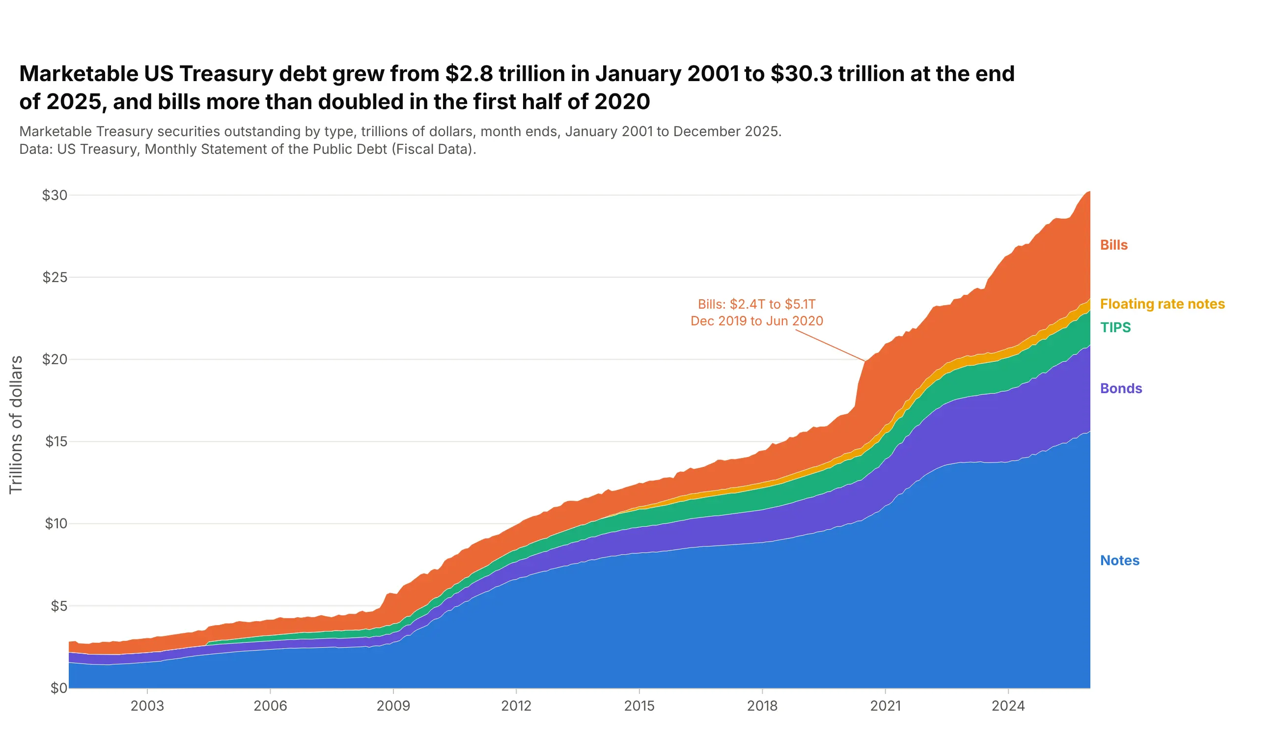
Stacked area chart of marketable US Treasury debt by type from 2001 to 2025: notes at the bottom, then bonds, TIPS, floating rate notes and bills on top. The total grows from $2.8 trillion to $30.3 trillion, and the bills band jumps from $2.4 trillion to $5.1 trillion in the first half of 2020

A total split by type. Marketable US Treasury debt grew from $2.8 trillion in January 2001 to $30.3 trillion at the end of 2025, and bills more than doubled, from $2.4 to $5.1 trillion, in the first half of 2020. Data: US Treasury, Monthly Statement of the Public Debt.

A short history

William Playfair is usually credited with the first area charts, in his 1786 Commercial and Political Atlas, which shaded the area between England's imports and exports to show the balance of trade (Wikipedia; Spence and Wainer, 2005). In 1821 he drew the price of wheat as bars over a shaded area of a mechanic's weekly wage. Here it is redrawn with Plotly from the values digitized from his chart:

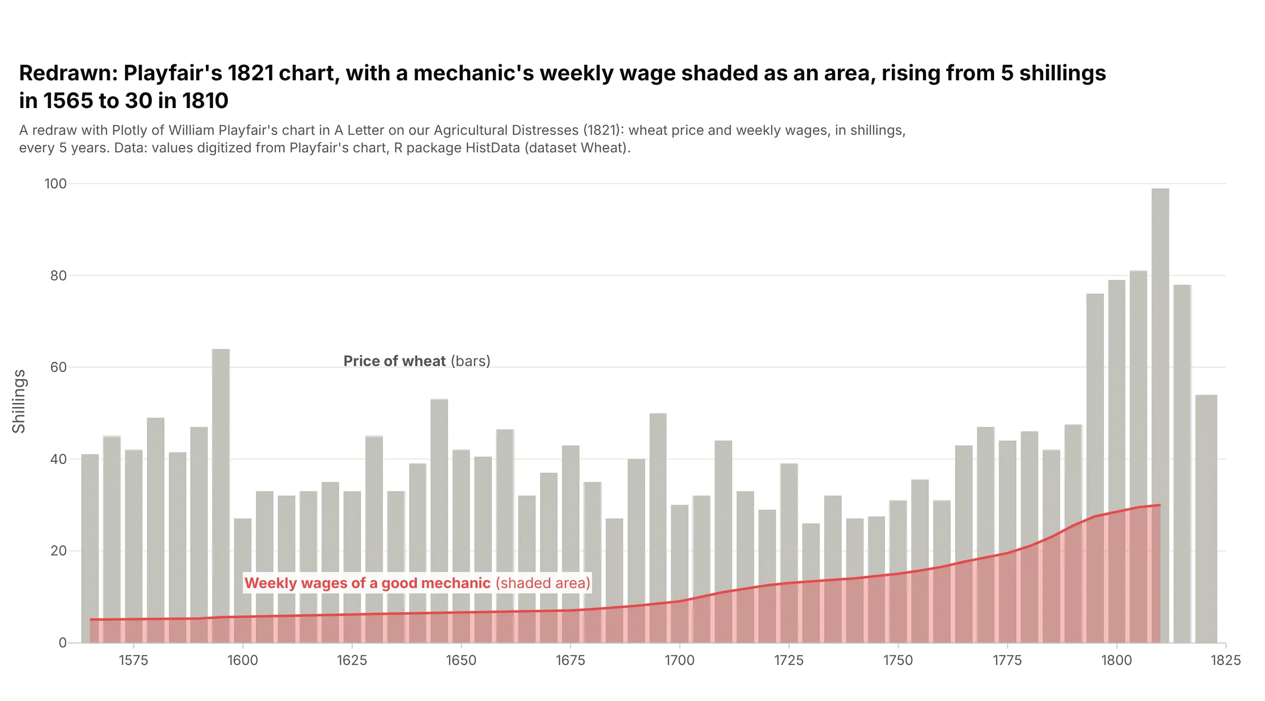
A redraw of Playfair's 1821 chart: gray bars for the price of wheat every five years from 1565 to 1821, peaking at 99 shillings in 1810, over a red shaded area of a mechanic's weekly wage rising from 5 shillings in 1565 to 30 in 1810

Data: R package HistData, dataset Wheat, digitized from Playfair (1821).

Alternatives to an area chart

Here's the same world energy data from 1965 to 2025 drawn six ways. Some are better for the question, some worse, some just different:

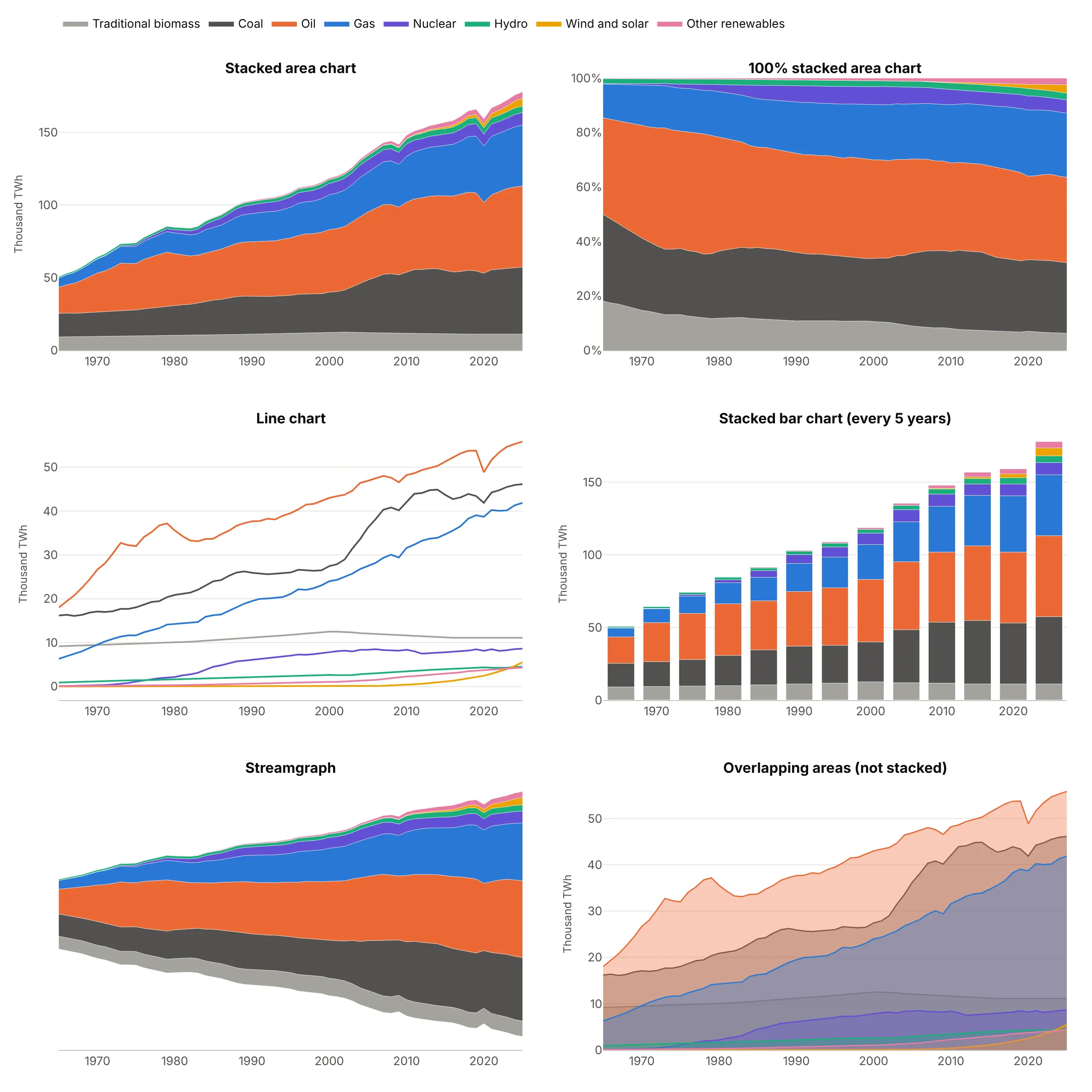
The same world primary energy by source from 1965 to 2025 drawn six ways: a stacked area chart, a 100% stacked area chart, a line chart, a stacked bar chart every five years, a streamgraph centered on a middle line, and overlapping unstacked areas where oil hides coal and gas

100% stacked area chart (better for shares). Every year adds up to 100%, so you can see oil's share shrink from 45% of the total in 1973 to 31% in 2025, but the growth of the total disappears.
Line chart (better for exact values). Each source starts from zero, so you can read that coal and gas both grew past 40,000 TWh. Eight lines are still readable; twenty would not be, and the total is gone.
Stacked bar chart (works too, for a few dates). The same stack every five years. It's easier to read one year exactly, and harder to follow a trend.
Streamgraph (worse here). The same layers around a center line instead of zero. It shows how the mix changes, but without a zero baseline you can't read the total, which is the point of this chart.
Overlapping areas (worse here). Each source filled to zero and drawn on top of the others, so oil hides coal and gas. Use it for two or three series you want to compare directly, as in way 5 below, not for parts of a whole.

How to make an area chart

With AI

ChatGPT, Claude Code, GitHub Copilot, Cursor and other AI tools are excellent at writing Plotly code. Name Plotly in the prompt, and say what order the layers go in and whether you want totals or shares:

Make a plotly stacked area chart from global_energy.csv (columns: year, traditional_biomass, coal, oil,
gas, nuclear, hydro, wind, solar, biofuels, other_renewables; TWh per year).

- Use px.area on the long table, one band per source, from traditional biomass at the bottom to the
  newest sources on top, wind and solar combined.
- Thin white lines between bands, one color per source, and labels at the right edge instead of a legend.
- A y axis from zero in TWh with thousands separators, and a title that states the takeaway.
- Then a second version with groupnorm="percent".
- Check: print the total and each source's share in the first and last year.

With Plotly Studio

Plotly Studio is a desktop app where you point an AI at a dataset and it builds charts and a Dash app around your questions. Ask for an area chart the same way:

Show a stacked area chart of world population by age group from 1950 to 2100, youngest at the bottom, with the UN projection years shaded, and a toggle between people and percent of the total.

Make an area chart in Python or JavaScript

This is the code AI tools write under the hood. In Python, px.area makes a stacked area chart in one line of code, and groupnorm="percent" makes the 100% version. The Plotly filled area chart documentation covers more options:

import pandas as pd
import plotly.express as px

df = pd.read_csv("global_energy.csv")  # year, traditional_biomass, coal, oil, gas, nuclear, hydro, wind, solar, ...
long = df.melt(id_vars="year", var_name="source", value_name="twh")

fig = px.area(long, x="year", y="twh", color="source",
              labels={"year": "", "twh": "TWh per year", "source": "Source"},
              title="World primary energy consumption by source")
fig.update_yaxes(tickformat=",")
fig.show()

# the same data as shares: every year adds up to 100%
fig = px.area(long, x="year", y="twh", color="source", groupnorm="percent")
fig.update_yaxes(ticksuffix="%", title="Share of world energy")
fig.show()

px.area returns one go.Scatter trace per color, all in the same stackgroup, which is what stacks them. To build it trace by trace, give every go.Scatter the same stackgroup="...". For a single area that isn't stacked, use go.Scatter(fill="tozeroy"), and for a band between two lines, fill="tonexty" on the second one.

In JavaScript, a plotly.js area chart is a set of scatter traces with the same stackgroup. Uncomment groupnorm for a 100% stacked area chart:

<div id="chart"></div>
<script src="https://cdn.plot.ly/plotly-4.1.1.min.js"></script>
<script>
  // World population by age group, billions (UN World Population Prospects; 2025 on are projections)
  const years = [1950, 1975, 2000, 2025, 2050, 2075, 2100];
  const groups = {
    "Under 15":    [0.87, 1.51, 1.88, 2.01, 1.97, 1.85, 1.68],
    "15 to 24":    [0.46, 0.76, 1.10, 1.28, 1.28, 1.26, 1.19],
    "25 to 64":    [1.04, 1.57, 2.78, 4.08, 4.84, 5.00, 4.88],
    "65 and over": [0.13, 0.23, 0.42, 0.86, 1.58, 2.13, 2.42]
  };

  const traces = Object.entries(groups).map(([name, y]) => ({
    x: years, y: y, name: name, type: "scatter", mode: "lines",
    stackgroup: "age",                       // same stackgroup = stacked areas
    // groupnorm: "percent",                 // a 100% stacked area chart
    line: {width: 0.5}
  }));

  Plotly.newPlot("chart", traces, {
    width: 800, height: 450, title: {text: "World population by age group"},
    yaxis: {title: {text: "Billion people"}}, hovermode: "x unified"
  });
</script>

In React, pass the same traces to the Plot component from react-plotly.js:

import Plot from "react-plotly.js";

export default function StackedArea({ years, groups }) {
  const data = Object.entries(groups).map(([name, y]) => ({
    x: years, y, name, type: "scatter", mode: "lines", stackgroup: "one"
  }));
  return <Plot data={data} layout={{ title: { text: "World population by age group" } }} />;
}

Share it

Every Plotly chart has a Share chart button (the cloud icon in its toolbar) that uploads it to Plotly Cloud and gives you a link. Only you can see it until you change its visibility.

For a live app, put the chart in a Dash app and publish it with the Plotly Cloud CLI. Coding agents can run these commands for you:

pip install "dash[cloud]"
plotly user login
plotly app publish

If your data has to stay in your own cloud or data center, publish to Dash Enterprise instead.

Dos and don'ts

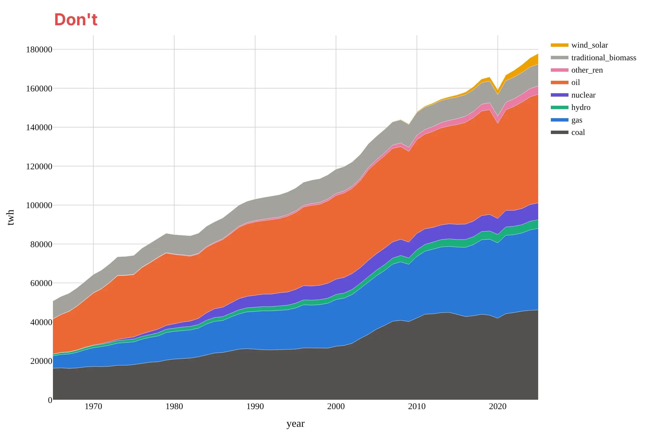
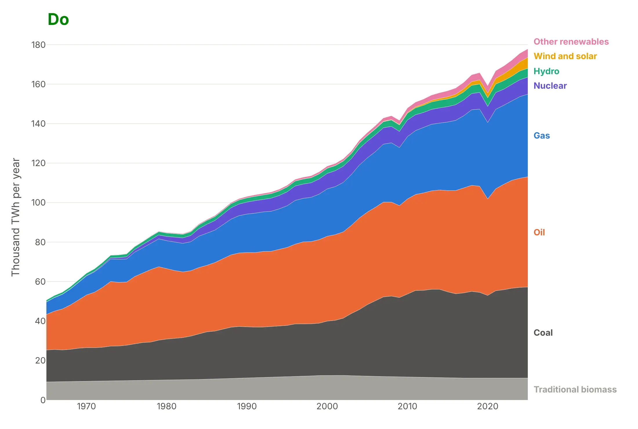
Most of the work in a published stacked area chart is choosing the order of the layers and labeling them. Here is world energy from 1965 to 2025 both ways, in the same colors.

Don't stack the layers in alphabetical order, so oil and gas sit on coal and every band above them inherits their swings, use raw column names in a legend that lists the layers in the opposite order to the stack, leave the tick numbers unformatted with a raw axis title, or use a default serif font:

World energy from 1965 to 2025 as a stacked area chart with layers in alphabetical order (coal, gas, hydro, nuclear, oil, other renewables, traditional biomass, wind and solar from the bottom), raw column names in a legend, unformatted tick labels up to 180000, the axis titles year and twh, and a serif font

Do put the big, steady layers at the bottom and the small or new ones on top, in an order that means something (here, when each fuel arrived), label each layer at the right edge in stack order, and give the axis a unit and formatted numbers:

The same data with traditional biomass at the bottom, then coal, oil, gas, nuclear, hydro, wind and solar and other renewables, each labeled at the right edge in its own color, and the y axis in thousand TWh per year

Checklist

Stack only parts that add up to a meaningful total, and start the y axis at zero.
Put the largest or steadiest layer at the bottom and the most volatile or newest on top.
Keep it to about eight layers, and combine the small ones into "Other".
Label layers directly at the right edge, or keep the legend in the same order as the stack.
Use groupnorm="percent" when the question is about shares, and say so in the title.
Shade or hatch projected years, as in the population example above.

Don't

Stack series that overlap, such as deaths by drug when one death can involve several drugs.
Stack negative values with positive ones in the same group; put them in their own stackgroup below zero.
Use spline smoothing on stacked data; it can bend layers below zero or past the total.
Read a middle layer's top edge as its value; read its thickness.

Options to customize

An area chart in Plotly is px.area or go.Scatter traces with a fill, so these are the options that matter most. The full lists are in the px.area reference and the scatter trace reference.

px.area(x=..., y=..., color=...): one stacked band per value of color, from a long table.
groupnorm="percent" (or "fraction"): rescales each x to a 100% stacked area chart; in go.Scatter set it on the first trace of the group.
stackgroup: traces with the same name stack; put negative values in a second group so they stack down from zero.
fill: "tozeroy" for a single area, "tonexty" for a band between two traces, "toself" for a closed shape.
fillcolor: the band color; use rgba with transparency for overlapping areas.
line.width, line.color: thin white lines between stacked bands, or no line at all.
line.shape: "hv" for a step area chart (rates, targets, prices that change on a date), "spline" for smooth single areas.
stackgaps: "infer zero" (the default) treats a missing value as zero, "interpolate" joins across it.
category_orders or trace order: the order of the layers, bottom first.
fillpattern: hatching, for projections or estimates.
hovermode="x unified": one tooltip with every layer's value at that x.
add_vrect, add_annotation: shaded periods (recessions, projections) and labels at the right edge.

12 ways to draw an area chart

The same data can make a dozen different area charts, and each one answers a different question. We took 25 years of monthly US electricity generation by source, 300 months from January 2001 to December 2025 with a summer peak every year and a fuel switch from coal to gas, and drew it 12 ways.

1. A single filled area

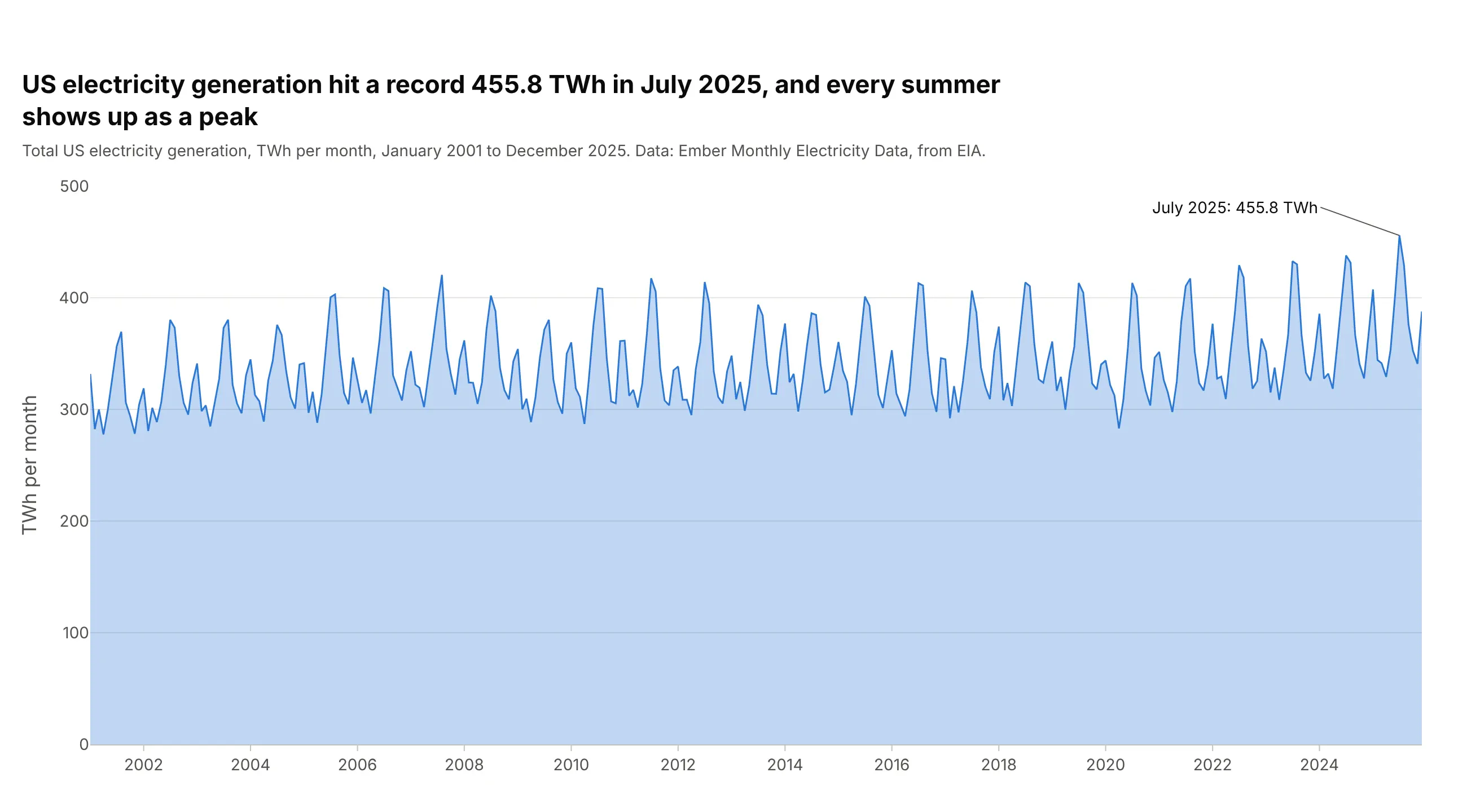
Area chart of total US electricity generation by month from 2001 to 2025, filled in light blue from zero, with a peak every summer and a record of 455.8 TWh in July 2025

The simplest area chart is one series filled down to zero, which makes the amount feel like a quantity rather than a trend line. Every summer shows up as a peak, and the record was 455.8 TWh in July 2025. It hides what the total is made of, and because the fill starts at zero, small changes look small. In Plotly it's go.Scatter(fill="tozeroy"), or px.area with one series.

Prompt: Get the data from Ember's Monthly Electricity Data (based on EIA's Electric Power Monthly), United States, total generation in TWh per month, 2001-2025. Make a plotly area chart with go.Scatter(fill="tozeroy"), a light blue fill and a darker line, a y axis from zero, the record month labeled with an arrow, and a title that states the record.

2. A stacked area chart

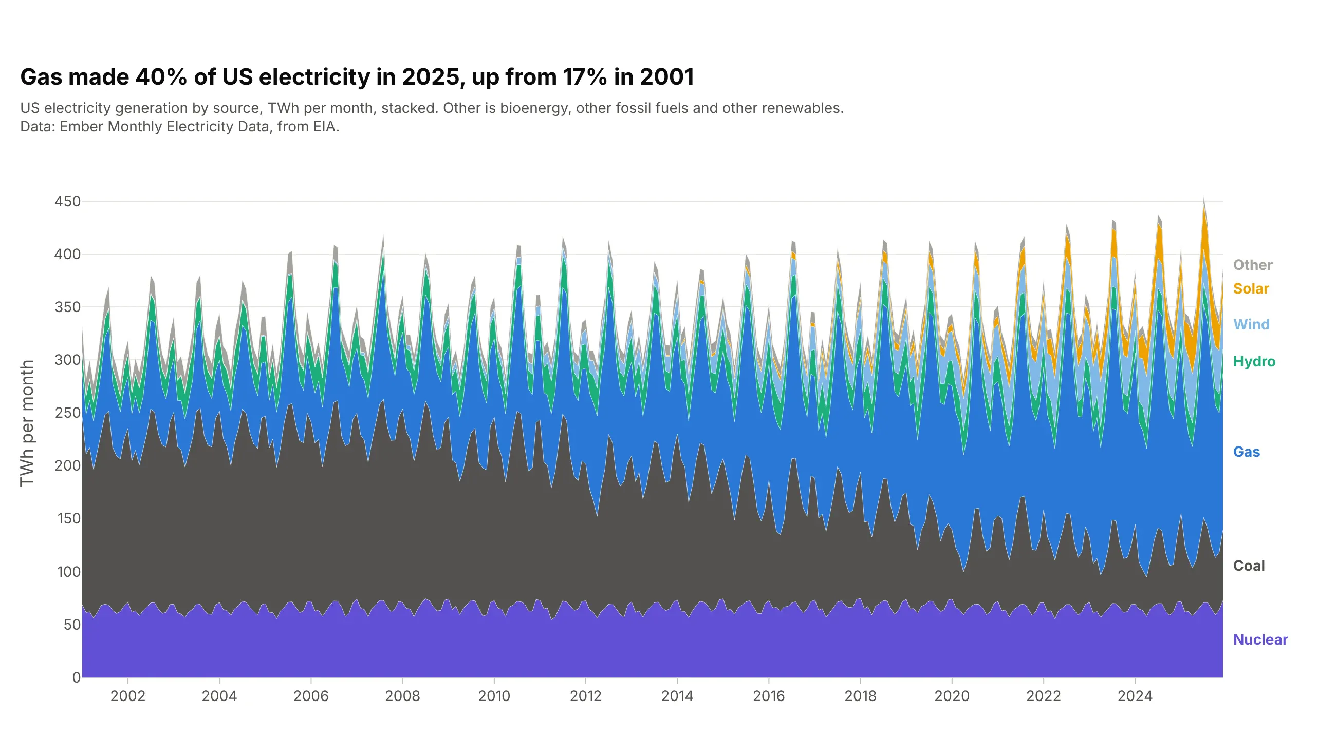
Stacked area chart of US electricity generation by source by month from 2001 to 2025: nuclear at the bottom, then coal, which shrinks, gas, which grows into the biggest band, and hydro, wind, solar and other on top

Stacking the sources keeps the total as the top edge and shows what it is made of. Gas made 40% of US electricity in 2025, up from 17% in 2001, and you can see its band take the room coal gave up. The steady nuclear band goes at the bottom so the others don't wobble on it. px.area(df, x="date", y="twh", color="source") puts every source in one stackgroup.

Prompt: Get the data from Ember's Monthly Electricity Data (from EIA), United States, generation by fuel in TWh per month, 2001-2025, with bioenergy, other fossil and other renewables combined as Other. Make a plotly stacked area chart with px.area and color="source", nuclear at the bottom, then coal, gas, hydro, wind, solar and Other, thin white lines between bands and labels at the right edge.

3. A 100% stacked area chart

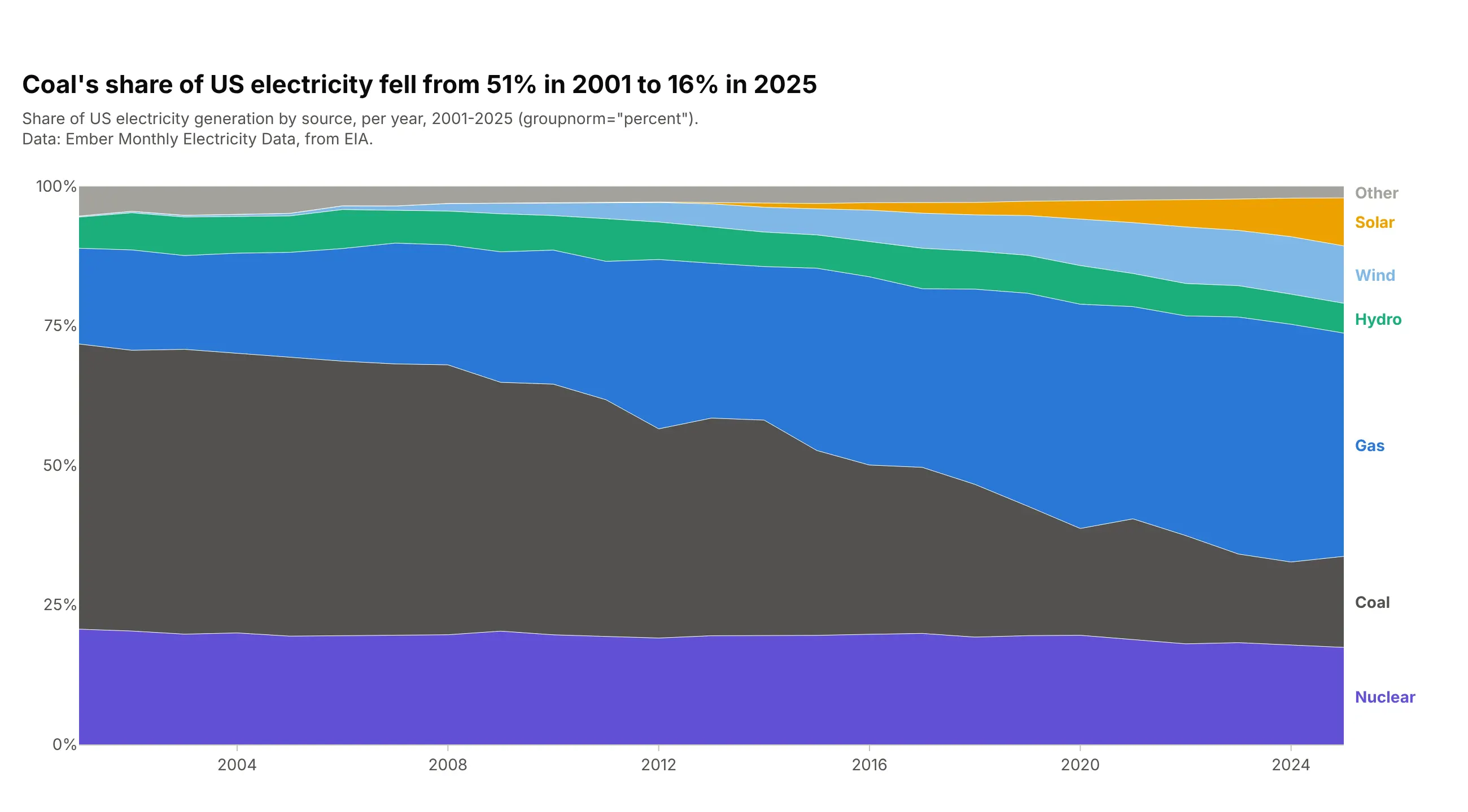
100% stacked area chart of the share of US electricity by source per year from 2001 to 2025: coal's dark band shrinks from about half to a sixth while gas grows to 40% and wind and solar appear at the top

When the question is about shares, scale every year to 100%. Coal's share fell from 51% in 2001 to 16% in 2025. The growth of the total disappears, so use this next to a stacked chart when both matter. In Plotly, add groupnorm="percent" to px.area, and use yearly sums so the seasons don't add noise to the shares.

Prompt: Get the data from Ember's Monthly Electricity Data (from EIA), United States, generation by fuel in TWh per month, 2001-2025, and sum it by year. Make a plotly 100% stacked area chart with px.area(..., groupnorm="percent"), nuclear at the bottom and Other on top, a y axis from 0 to 100% and labels at the right edge.

4. A stacked area of 12-month rolling sums

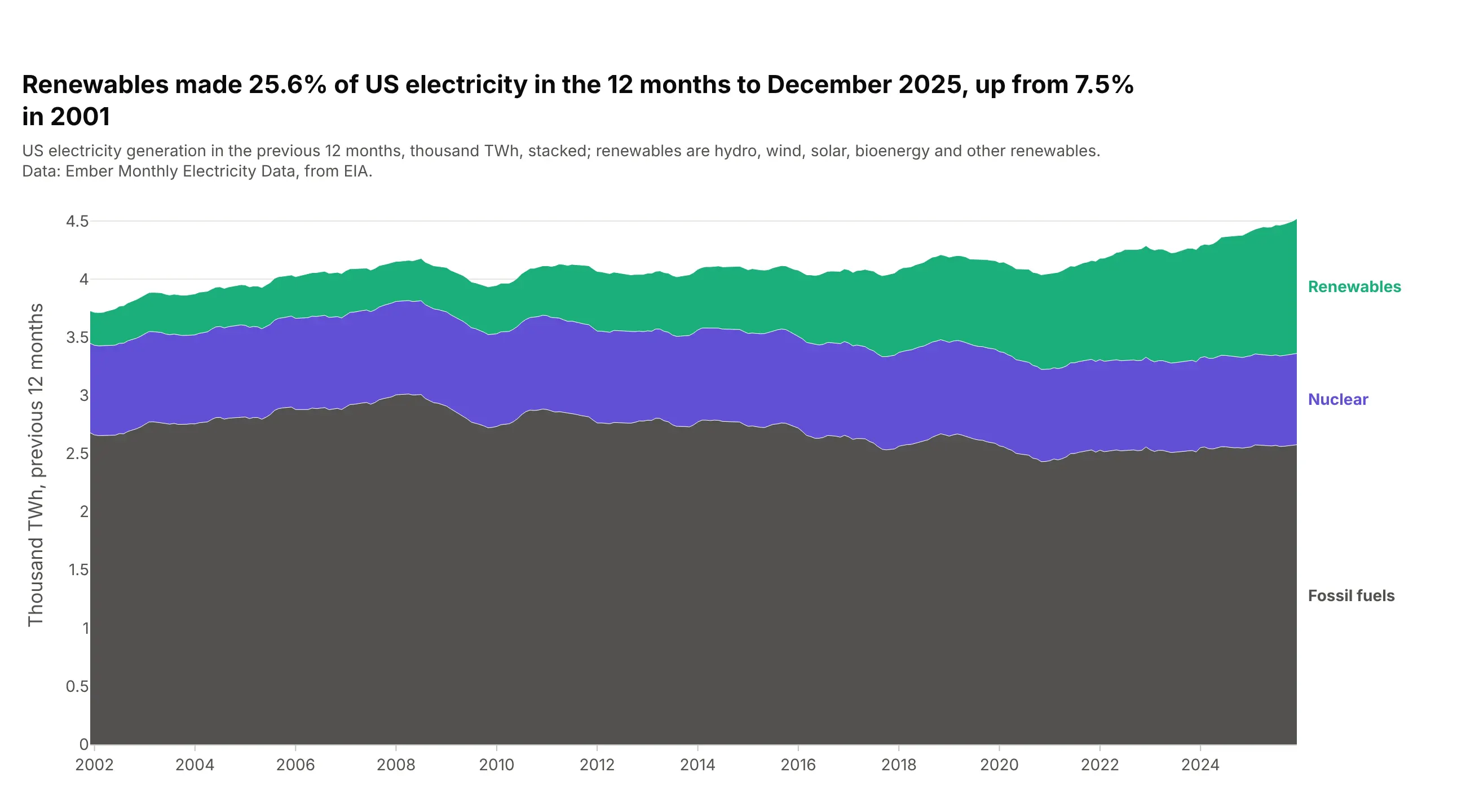
Stacked area chart of US electricity in the previous 12 months, 2001 to 2025, in three bands: fossil fuels at the bottom, nuclear, and renewables on top, which widen from about 0.3 to 1.2 thousand TWh

Monthly data with a strong season can be hard to read as a trend. A 12-month rolling sum takes the seasons out, so each point is the year to that month. Renewables made 25.6% of US electricity in the 12 months to December 2025, up from 7.5% in 2001. Compute it in pandas with .rolling(12).sum() and stack it with a shared stackgroup.

Prompt: Get the data from Ember's Monthly Electricity Data (from EIA), United States, generation by fuel in TWh per month, 2001-2025, and group it into fossil fuels, nuclear and renewables. Compute 12-month rolling sums with pandas .rolling(12).sum(). Make a plotly stacked area chart with go.Scatter traces in one stackgroup, fossil fuels at the bottom, and labels at the right edge.

5. Overlapping areas

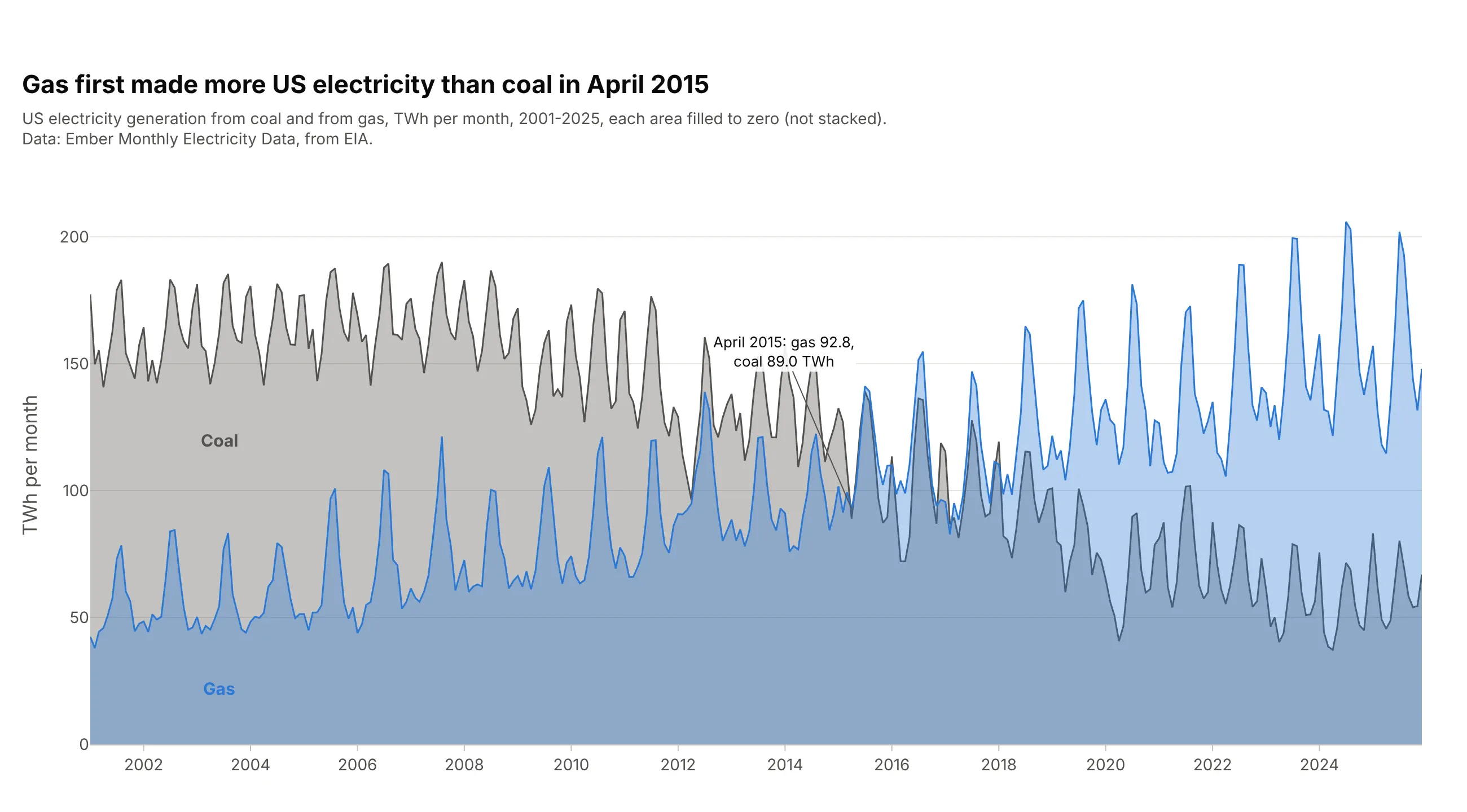
Two overlapping area charts of US electricity from coal in gray and from gas in blue, each filled to zero, from 2001 to 2025; the gas area rises above coal from 2015 and stays above it from 2018

To compare two series head to head, fill each one to zero with a transparent color instead of stacking them. Gas first made more electricity than coal in April 2015, at 92.8 TWh against 89.0. Two or three series work; more than that and the colors turn muddy. Use fill="tozeroy" on each go.Scatter and an rgba fill color at 0.3 to 0.4 opacity.

Prompt: Get the data from Ember's Monthly Electricity Data (from EIA), United States, coal and gas generation in TWh per month, 2001-2025. Make a plotly chart of two overlapping areas, not stacked: each go.Scatter with fill="tozeroy", coal in gray and gas in blue, both fills at 35% opacity, labels inside each area, and the first month gas beat coal labeled.

6. Positive and negative fills

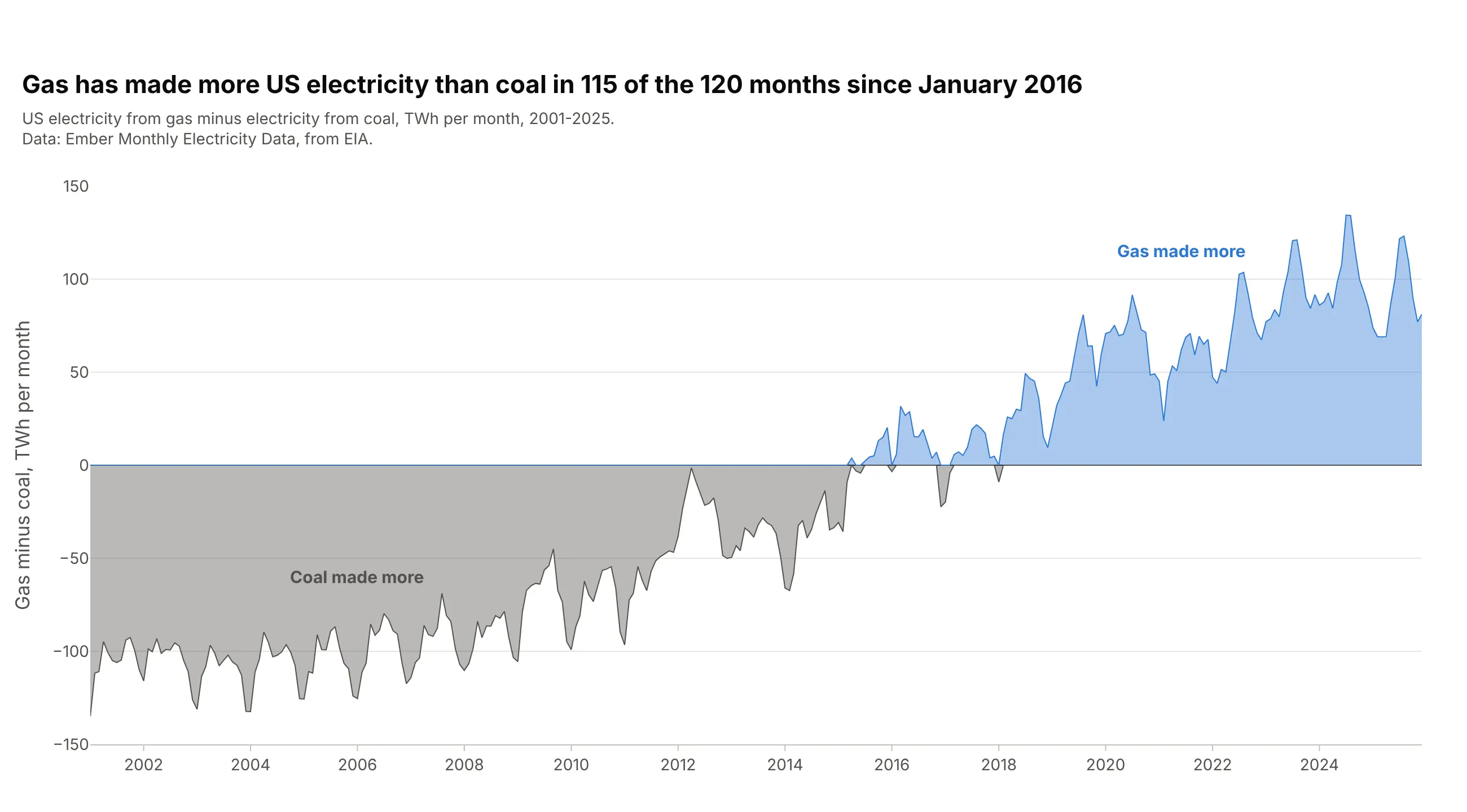
Area chart of US electricity from gas minus coal by month from 2001 to 2025, gray below zero until 2015 and blue above zero after it, with a few gray dips in 2015 to 2018

Plot the difference between two series and color the area by its sign. Gas made more electricity than coal in 115 of the 120 months from January 2016 to December 2025, and the last month coal came out ahead was January 2018. It shows the gap and the crossover exactly, but not the size of either series. Split the difference into a positive and a negative copy with clip(lower=0) and clip(upper=0) and fill each to zero.

Prompt: Get the data from Ember's Monthly Electricity Data (from EIA), United States, coal and gas generation in TWh per month, 2001-2025, and compute gas minus coal. Make a plotly area chart of the difference, split with clip into a positive trace in blue and a negative trace in gray, each with fill="tozeroy", a black zero line, and labels for which fuel made more.

7. A range band with this year on top

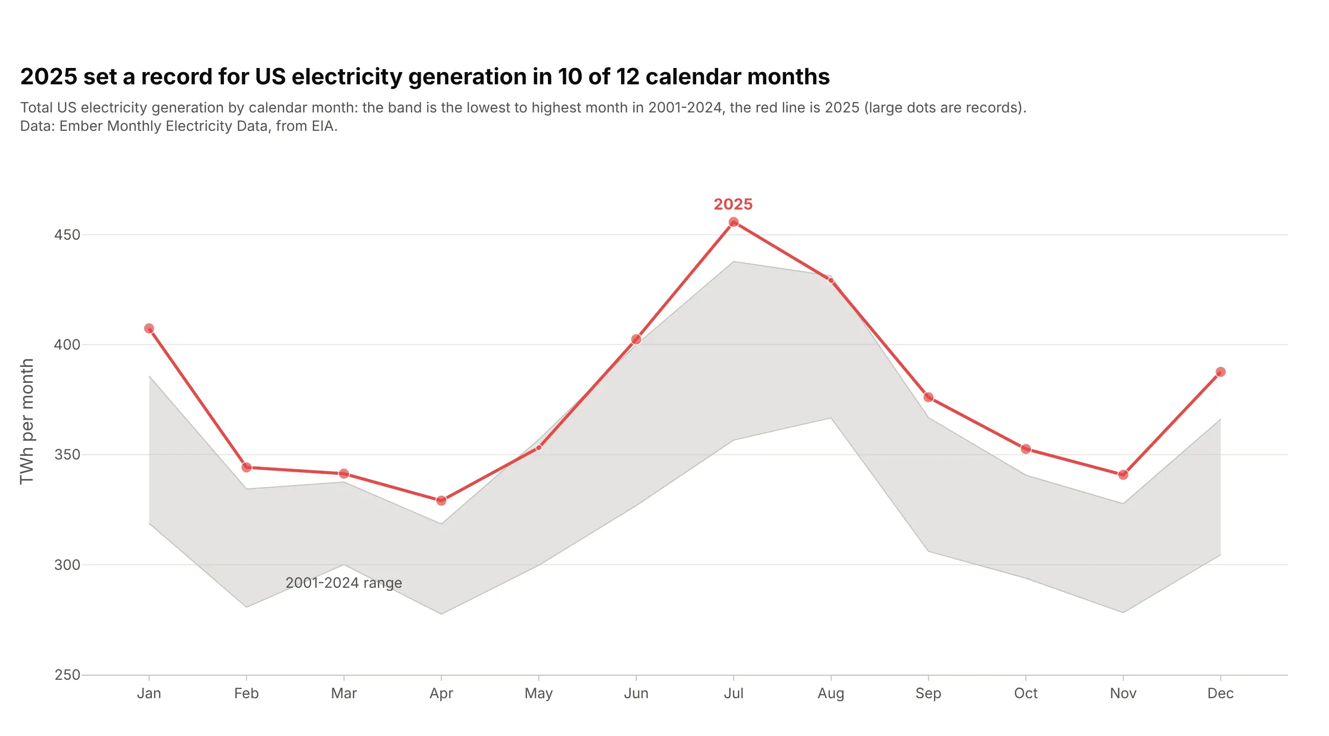
Area band of the lowest to highest US electricity generation for each calendar month in 2001 to 2024, in light gray, with 2025 as a red line above the band in 10 of the 12 months

A band from the lowest to the highest value in past years, with the current year drawn over it, shows at a glance whether this year is normal. 2025 set a record for US electricity generation in 10 of 12 calendar months; only May and August stayed inside the 2001-2024 range. Draw the minimum as a plain line and the maximum with fill="tonexty", which fills down to the trace before it.

Prompt: Get the data from Ember's Monthly Electricity Data (from EIA), United States, total generation in TWh per month, 2001-2025. For each calendar month, compute the minimum and maximum over 2001-2024. Make a plotly chart with the minimum as a line and the maximum with fill="tonexty" as a gray band, 2025 as a red line with bigger markers on record months.

8. A year-over-year overlay

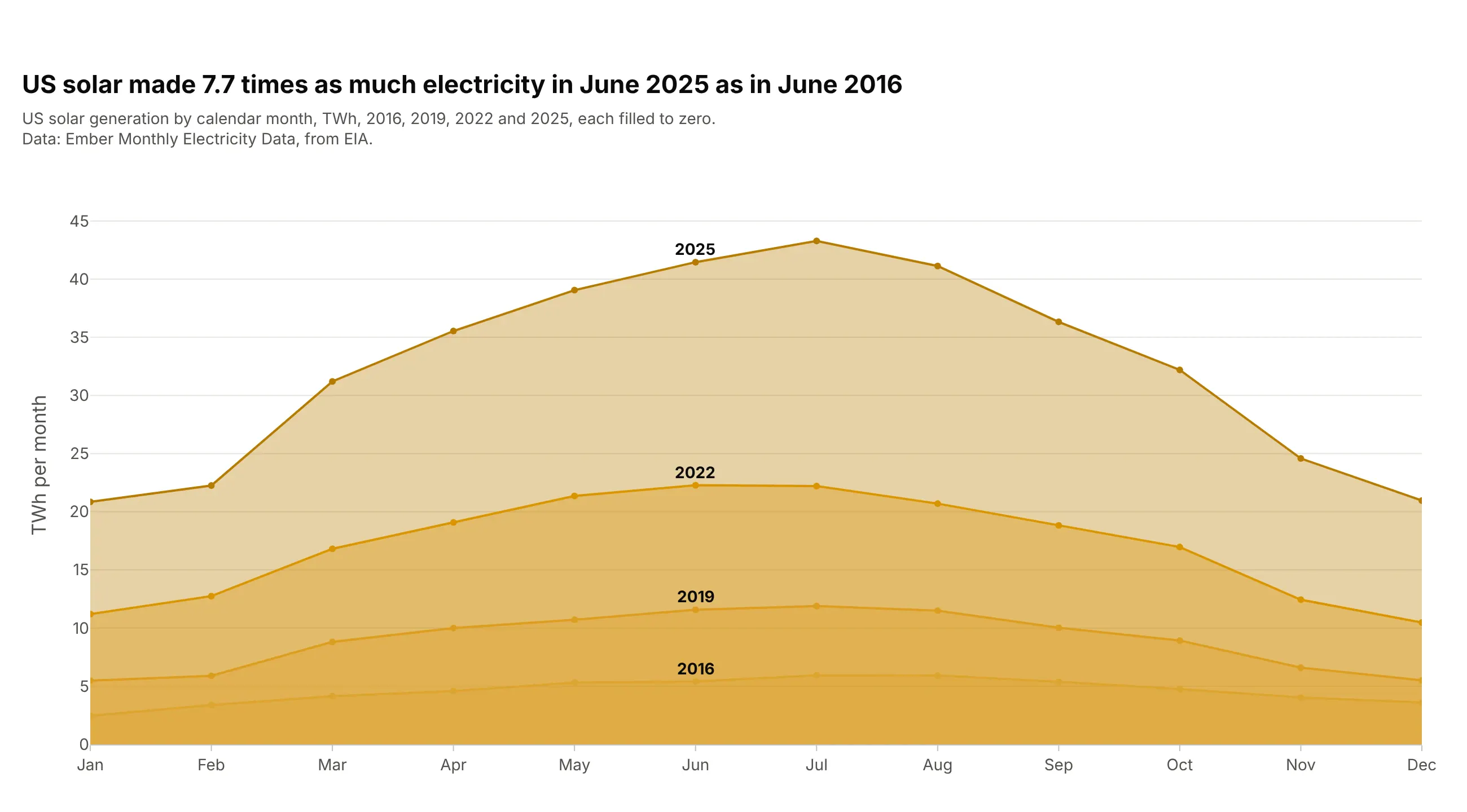
Four overlapping area charts of US solar generation by calendar month for 2016, 2019, 2022 and 2025, in shades of yellow, each one much taller than the last, with June 2025 at 41.5 TWh

Put calendar months on the x axis and draw one area per year to compare seasons and growth at once. US solar made 7.7 times as much electricity in June 2025 as in June 2016, and every year has the same summer hump. Keep it to a few years, with see-through fills so the smaller, older years show through the newest one. Each year is its own go.Scatter(fill="tozeroy") on a categorical month axis.

Prompt: Get the data from Ember's Monthly Electricity Data (from EIA), United States, solar generation in TWh per month, for 2016, 2019, 2022 and 2025. Make a plotly chart with months Jan to Dec on the x axis and one overlapping area per year, each go.Scatter with fill="tozeroy" in a darker shade of yellow for later years, and the year labeled at June.

9. A smoothed (spline) area

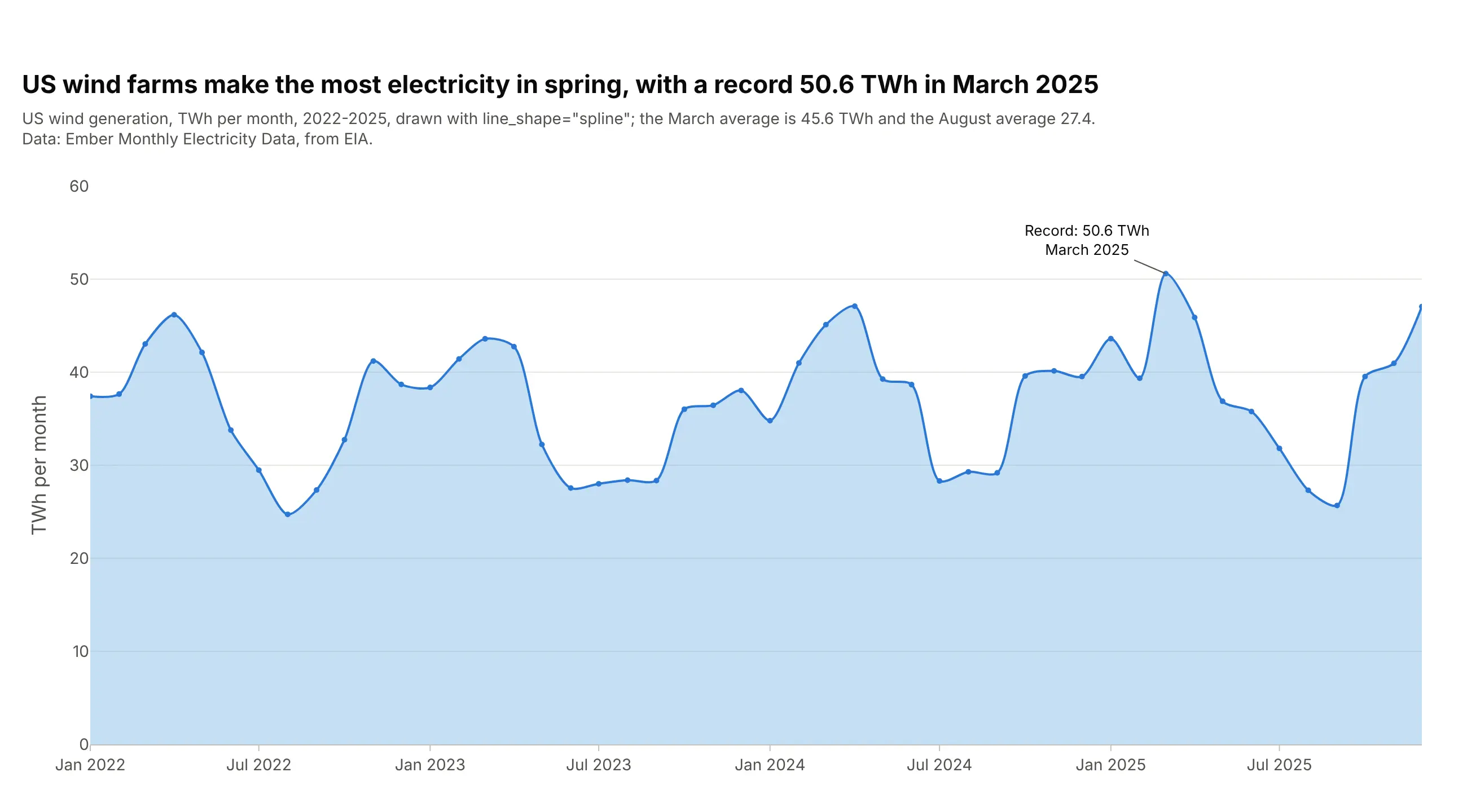
Spline area chart of US wind generation by month from 2022 to 2025, a smooth blue curve that peaks every spring and dips every late summer, with a record of 50.6 TWh in March 2025

A spline curve looks calmer than straight segments and suits a single series with a clear rhythm. US wind farms make the most electricity in spring, with a record 50.6 TWh in March 2025; from 2022 to 2025 the March average was 45.6 TWh and the August average 27.4. Keep the markers so readers see the real data points, because a spline can bend past them between months. In Plotly it's line_shape="spline".

Prompt: Get the data from Ember's Monthly Electricity Data (from EIA), United States, wind generation in TWh per month, 2022-2025. Make a plotly area chart with go.Scatter(fill="tozeroy", line_shape="spline", mode="lines+markers"), a light blue fill, small markers on the real monthly values so readers see where the curve is measured, the record month labeled with an arrow, and the March and August averages in the subtitle.

10. A step area chart

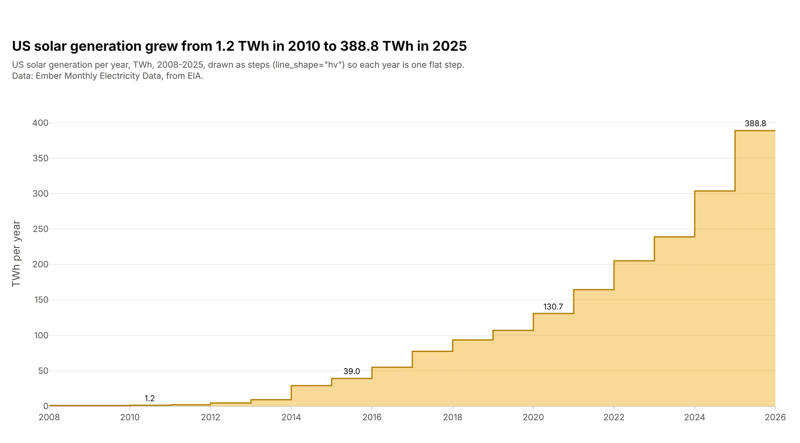
Step area chart of US solar generation per year from 2008 to 2025, one flat yellow step per year, rising from 1.2 TWh in 2010 to 39.0 in 2015, 130.7 in 2020 and 388.8 in 2025

When each value holds for a whole period, such as a yearly total, a rate or a price that changes on a date, draw it as steps. US solar generation grew from 1.2 TWh in 2010 to 388.8 TWh in 2025, and each year is one flat step you can read off the axis. A sloped line between years would suggest values in between that don't exist. Use line_shape="hv" with the fill.

Prompt: Get the data from Ember's Monthly Electricity Data (from EIA), United States, solar generation in TWh per month, 2008-2025, and sum it by year. Make a plotly step area chart with go.Scatter(fill="tozeroy", line_shape="hv"), repeating the last value one year later so 2025 gets a full step, and label 2010, 2015, 2020 and 2025.

11. Small multiples

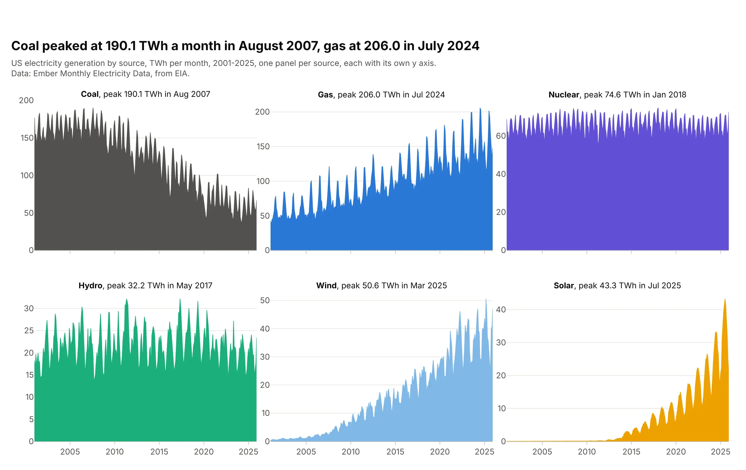
Six small area charts of US electricity by month from 2001 to 2025, one each for coal, gas, nuclear, hydro, wind and solar, each with its own y axis and its peak in the panel title

One small area per source, each with its own y axis, lets every series show its own shape instead of riding on the others. Coal peaked at 190.1 TWh a month in August 2007 and gas at 206.0 in July 2024, while nuclear stayed flat and most of solar's growth came after 2015. Separate y axes hide the relative sizes, so say so or share the axis when size matters. In Plotly it's px.area(..., facet_col="source", facet_col_wrap=3) with matches=None on the y axes.

Prompt: Get the data from Ember's Monthly Electricity Data (from EIA), United States, generation by fuel in TWh per month, 2001-2025, for coal, gas, nuclear, hydro, wind and solar. Make plotly small multiples with px.area(..., facet_col="source", facet_col_wrap=3), one color per source, independent y axes (fig.update_yaxes(matches=None)) and each panel titled with its peak month.

12. A cumulative area chart

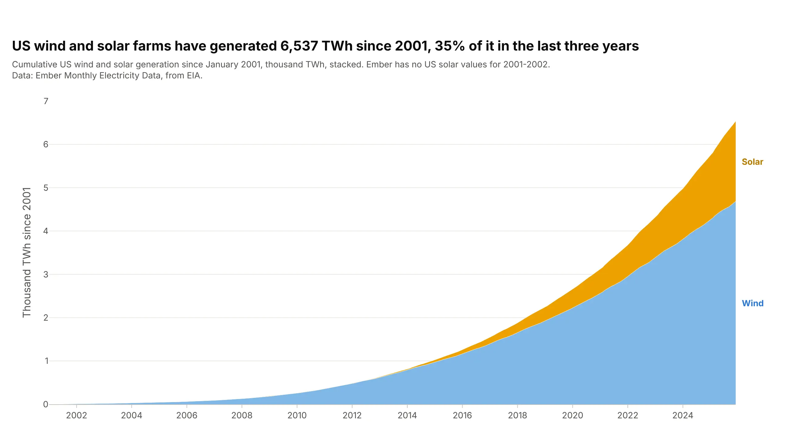
Cumulative stacked area chart of US wind and solar generation added up since January 2001, passing 1 thousand TWh in 2014 and rising steeply to 6.5 thousand TWh by December 2025, with solar a growing yellow band on top of wind

Adding the values up over time shows the total so far, which suits counts that only grow. US wind and solar farms have generated 6,537 TWh since 2001, 35% of it in the last three years. A cumulative chart always rises, so it hides slowdowns that a monthly chart would show. Compute it with pandas .cumsum() and stack the series in one stackgroup.

Prompt: Get the data from Ember's Monthly Electricity Data (from EIA), United States, wind and solar generation in TWh per month, 2001-2025. Compute running totals with pandas .cumsum(). Make a plotly stacked area chart of the cumulative values with go.Scatter traces in one stackgroup, wind at the bottom and solar on top, the y axis in thousand TWh, and labels at the right edge.