Dot Plots - A Complete Guide (with 12 Examples)

TL;DR

• A dot plot puts one dot per value on a common scale, one row per category, sorted. Several series per row, such as two years or three customer types, sit on the same line.
• Dot plots are also known as dot charts and Cleveland dot plots, and are similar to lollipop charts and dumbbell charts.
• Use one instead of a bar chart when the axis shouldn't start at zero, when the scale is logarithmic, or when you have two to five values per row.
• You can make a dot plot with Plotly from one go.Scatter in mode="markers" per series, with the categories on the y axis.
• Sort the rows, use dots without connecting lines, and put units on the axis.

What is a dot plot?

Dot plots look like this:

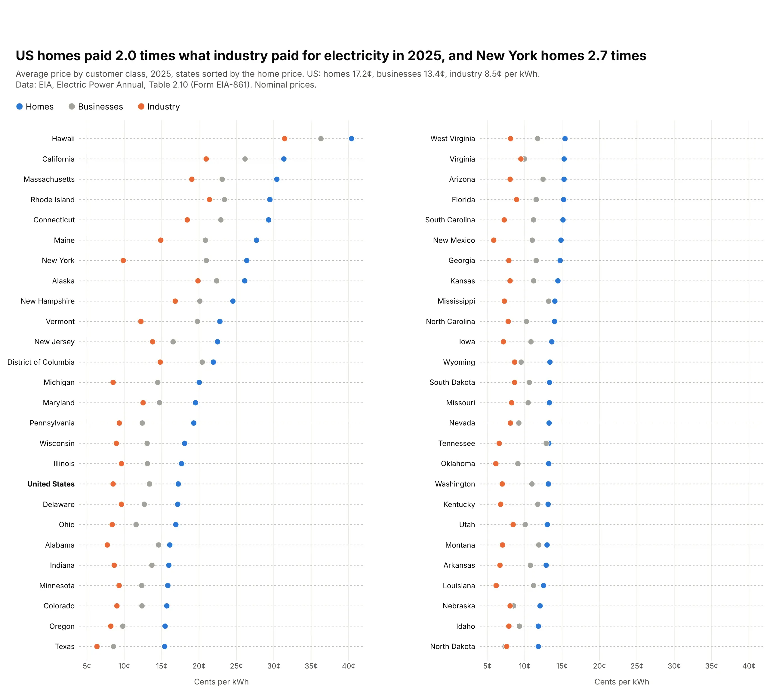
Data: EIA, Electric Power Annual, Table 2.10 (Form EIA-861), 2025.

How do you read a dot plot? In the example above, notice these things:

• Each row is one state, and each dot is the average price one kind of customer paid for electricity there in 2025, blue for homes, gray for businesses and orange for industry.
• The price is the dot's position along the axis, so nothing depends on a bar's length from zero and the axis can start near the cheapest price. That keeps the dots spread out enough to see small differences between states.
• Reading across one row compares customers in the same state. In New York the orange industry dot sits far to the left of the blue home dot, because homes paid 2.7 times as much, while Hawaii's three dots all sit at the far right because it was the most expensive state for every kind of customer, with the smallest gap between homes and industry relative to the price.
• Reading down the blue dots compares states, because the rows are sorted by the home price from Hawaii at the top of the left column to North Dakota at the bottom of the right one. The bold United States row gives you the national average to compare each state with.
• The two columns share the same axis, so the right column is the cheaper half of the list carried on. Watch for dots that overlap, like the gray and blue ones in Tennessee, which has the smallest gap between businesses and homes of any state, so one dot partly hides the other.

It's often used for charts like these:

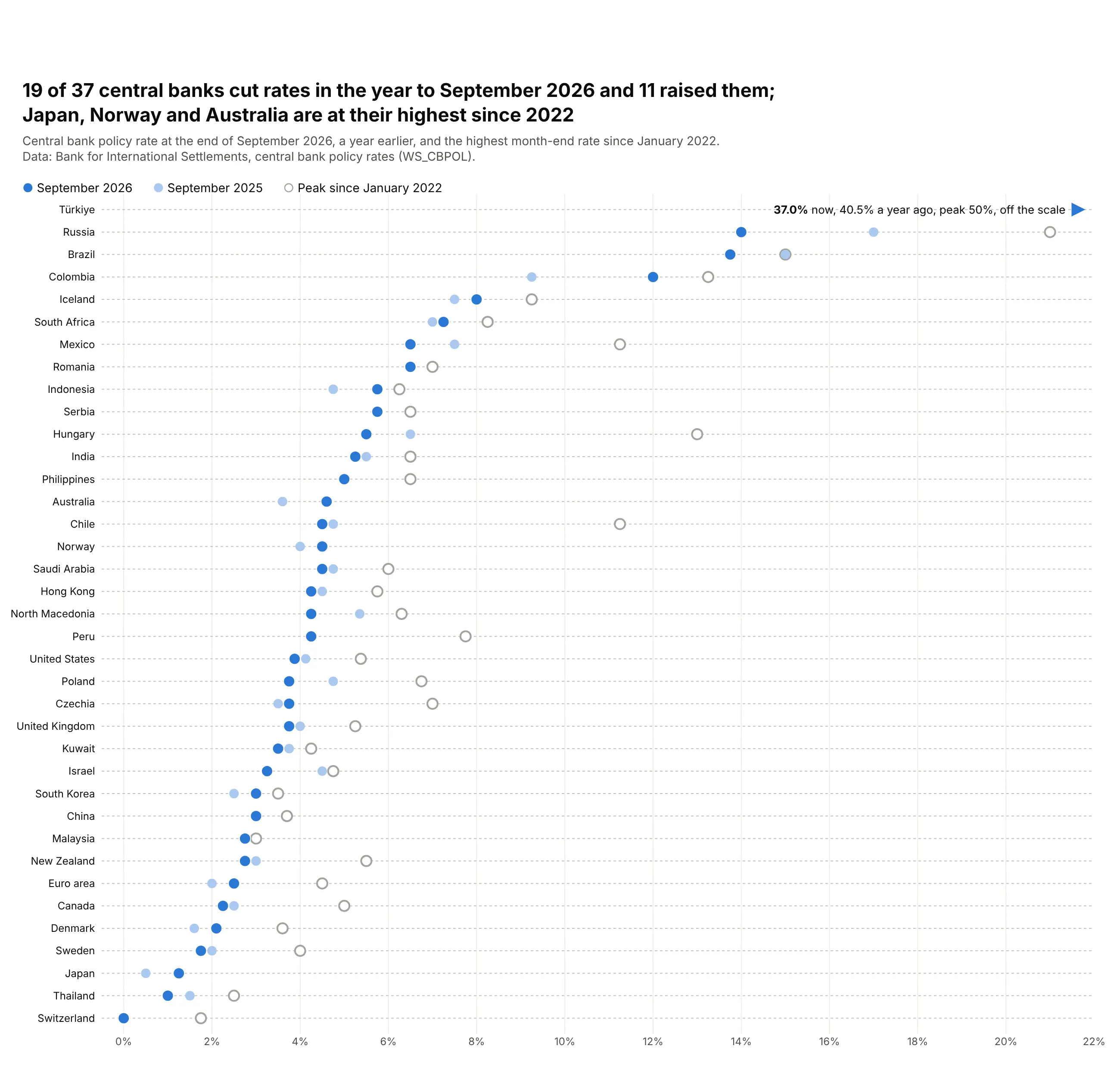
A current value against its history. 19 of 37 central banks cut rates in the year to September 2026, while Japan (1.25%), Norway (4.5%) and Australia (4.6%) are at their highest since 2022. Data: Bank for International Settlements, central bank policy rates.

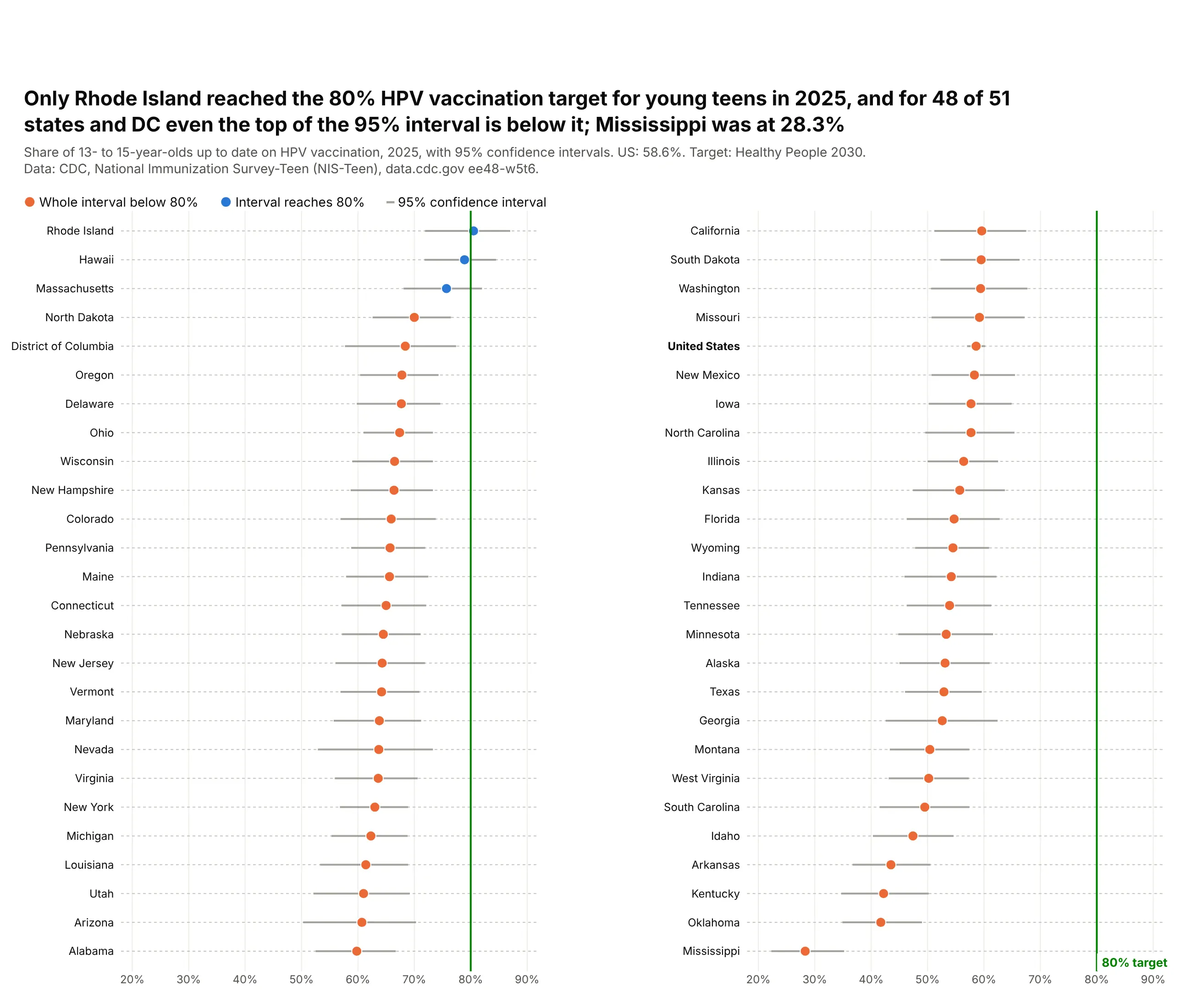
Survey estimates with their uncertainty. Only Rhode Island reached the 80% HPV vaccination target for young teens in 2025, and for 48 of 51 states and DC the whole 95% interval is below it. Data: CDC, National Immunization Survey-Teen.

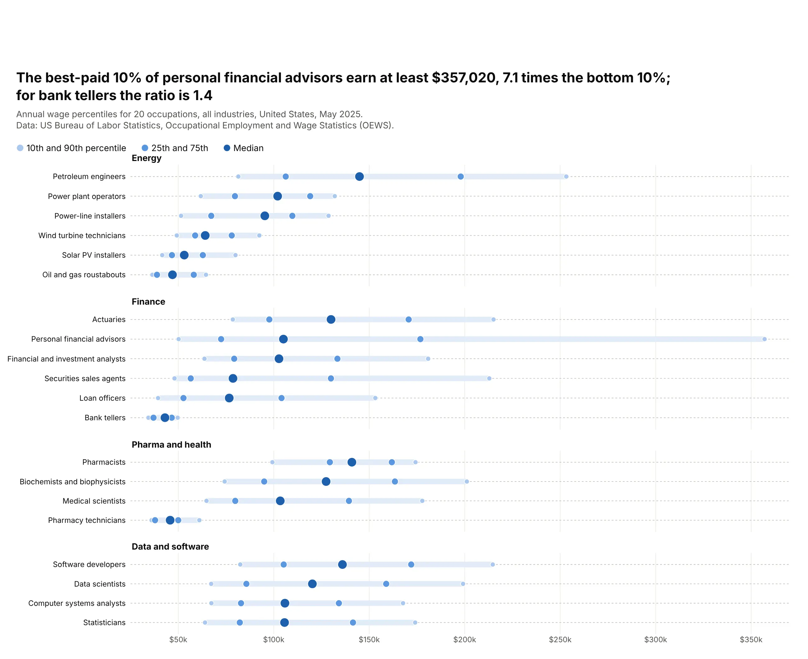
A distribution in five numbers. The best-paid 10% of personal financial advisors earn at least $357,020, 7.1 times what the bottom 10% earn, while for bank tellers the ratio is 1.4. Data: BLS, Occupational Employment and Wage Statistics, May 2025.

A short history

William Cleveland proposed the dot chart in 1984 as a replacement for bar charts and pie charts (Cleveland, 1984), after his experiments with Robert McGill showed that people judge positions on a common scale more accurately than lengths, angles or areas (Cleveland and McGill, 1984). His best-known example is in Visualizing Data (1993): barley yields from a 1930s Minnesota field trial (Immer, Hayes and Powers, 1934), drawn as a grid of dot plots. Here is that chart redrawn with Plotly from the original data:

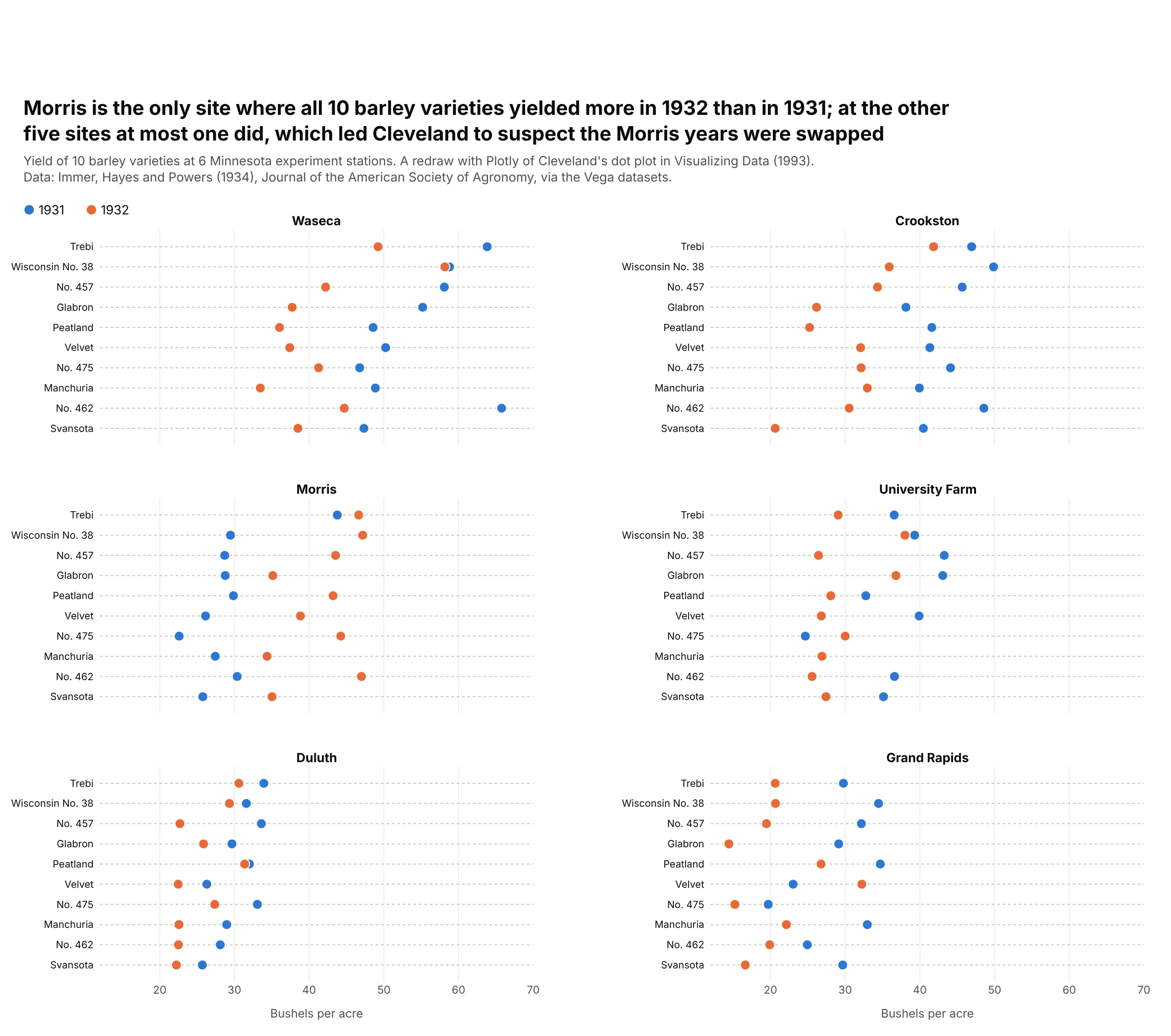
At Morris, every variety yielded more in 1932 than in 1931, while at every other site almost all of them yielded less. Cleveland suspected the two years had been swapped at Morris, something the printed tables had not made obvious. The name "dot plot" is also used for two other charts: the Wilkinson dot plot, a histogram made of stacked dots, and the Federal Reserve's "dot plot" of each official's rate projection. This guide is about Cleveland's version.

Alternatives to a dot plot

Here's the same time-use data drawn six ways. Some are better for the question, some worse, some just different:

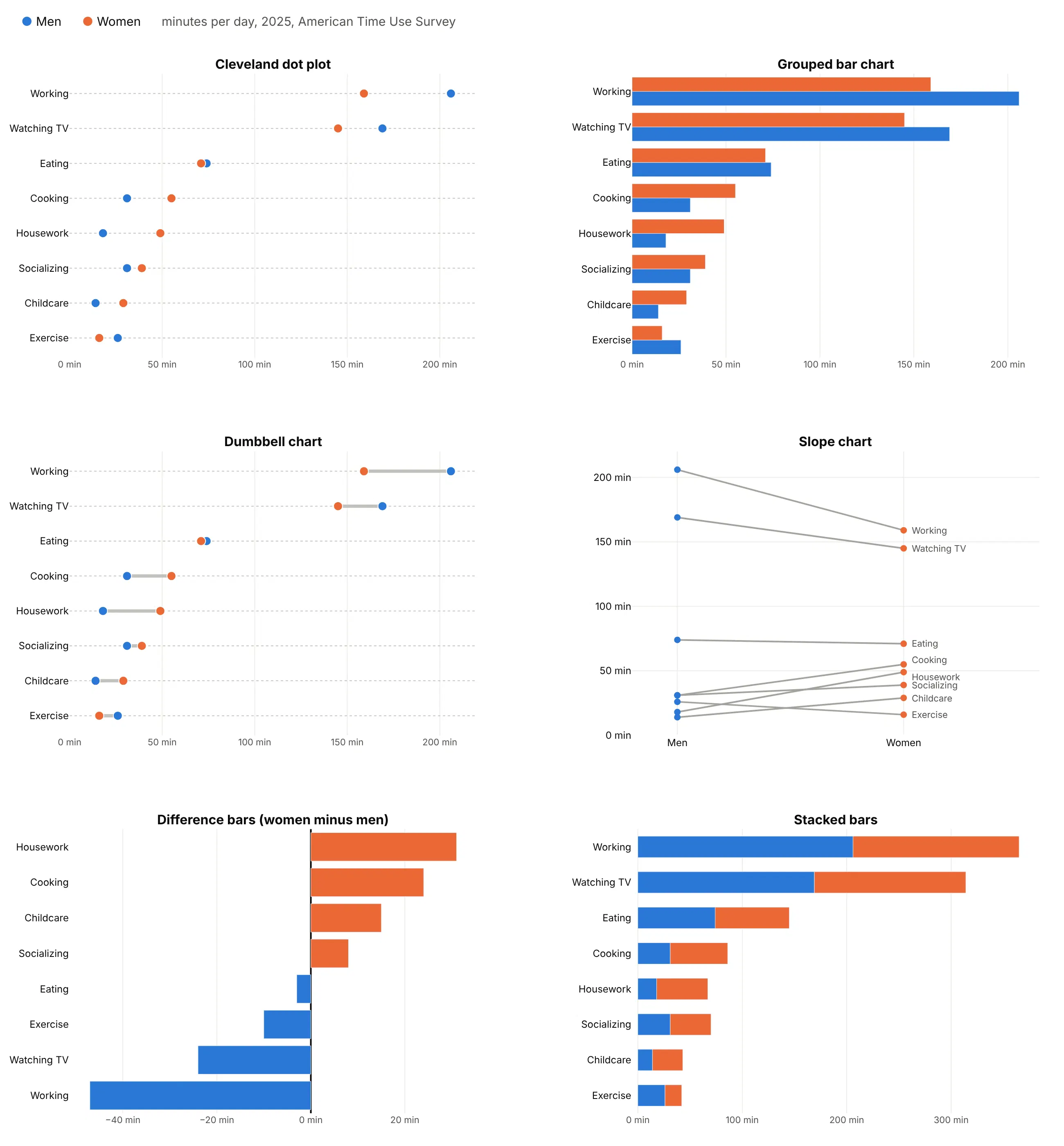
• Grouped bar chart (works too, when zero matters). Bars compare lengths from zero, which is right for counts and amounts. With two or more series the bars double the ink and the rows get tall, and a bar chart can't use a log axis or a zoomed axis.
• Dumbbell chart (better for the change between two values). The line between the two dots makes the gap the main thing you see. Use a dot plot for three or more series, or when the two values aren't a before and after. See our dumbbell chart guide.
• Lollipop chart (better for one series from zero). A dot on a thin stem from zero. Use it instead of a dot plot when there's one value per row and the length from zero means something. See our lollipop chart guide.
• Slope chart (different). Good for a few categories in two groups or two years, where the lines' angles and crossings are the story. With more than about ten rows the labels collide, as Cooking and Housework do here. See our slope chart guide.
• Difference bars (better when only the gap matters). One bar per row of women minus men. You lose the levels, so working (47 minutes) looks bigger than housework (31 minutes) without showing that work takes over three hours.
• Stacked bars (worse). Only the first segment starts at a common baseline, so the women's values can't be compared across rows.

How to make a dot plot

With AI

ChatGPT, Claude Code, GitHub Copilot, Cursor and other AI tools are excellent at writing Plotly code. Name Plotly in the prompt, say which columns are the rows and the series, and list the checks you want:

With Plotly Studio

Plotly Studio is a desktop app where you point an AI at a dataset and it builds charts and a Dash app around your questions. Ask for a dot plot the same way:

Show a dot plot of electricity prices by state with one dot each for homes, businesses and industry, sorted by the home price. Add a dropdown to choose which customer type to sort by.

Make a dot plot in Python or JavaScript

This is the code AI tools write under the hood. This small helper builds a dot plot from one go.Scatter per series, sorts the rows and draws the dotted row guides:

In JavaScript, plotly.js builds the same chart from two scatter traces:

For confidence intervals, add error_x=dict(type="data", array=..., arrayminus=..., width=0) to the marker trace, as in the HPV example above.

Share it

Every Plotly chart has a Share chart button (the cloud icon in its toolbar) that uploads it to Plotly Cloud and gives you a link. Only you can see it until you change its visibility.

For a live app, put the chart in a Dash app and publish it with the Plotly Cloud CLI. Coding agents can run these commands for you:

If your data has to stay in your own cloud or data center, publish to Dash Enterprise instead.

Dos and don'ts

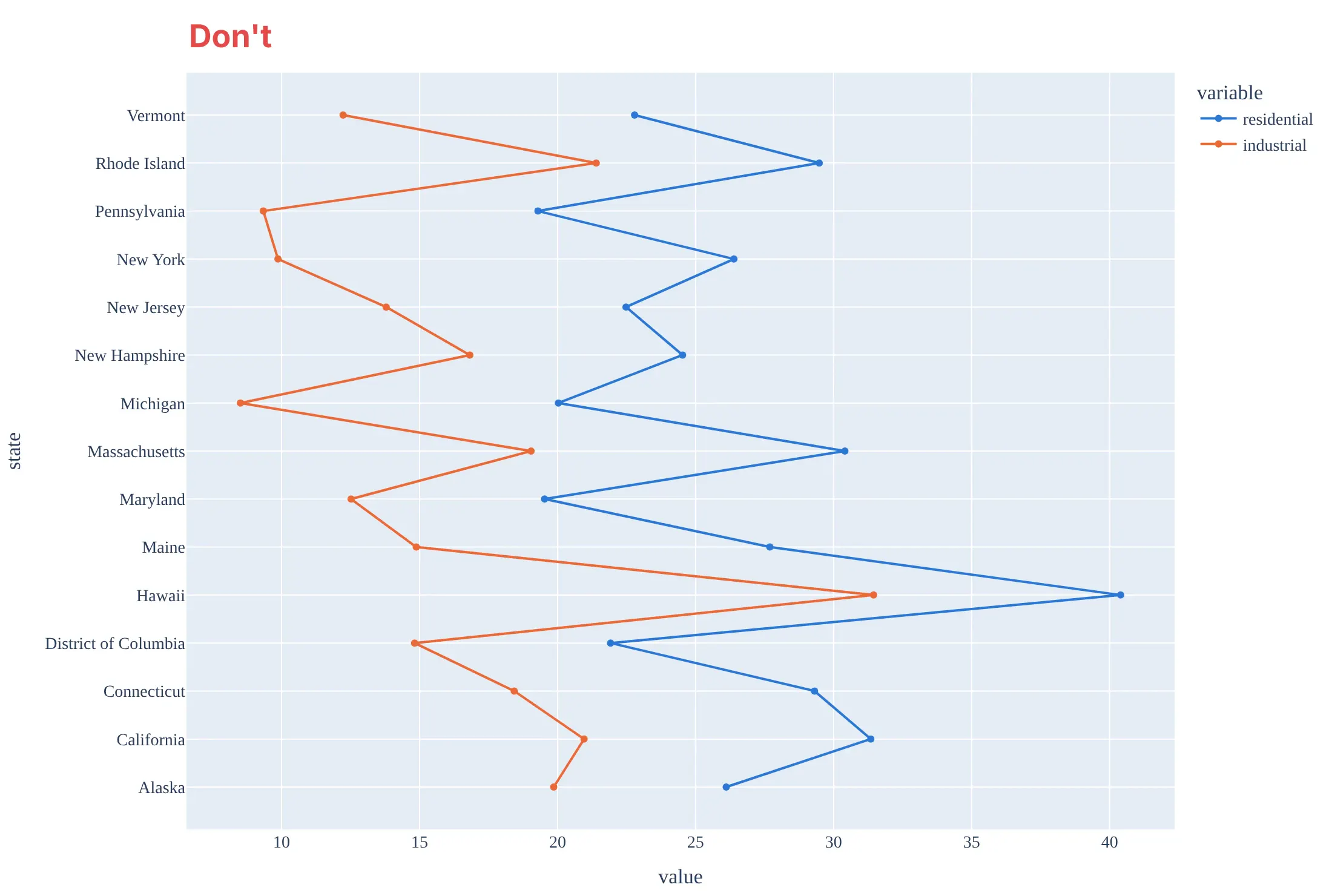
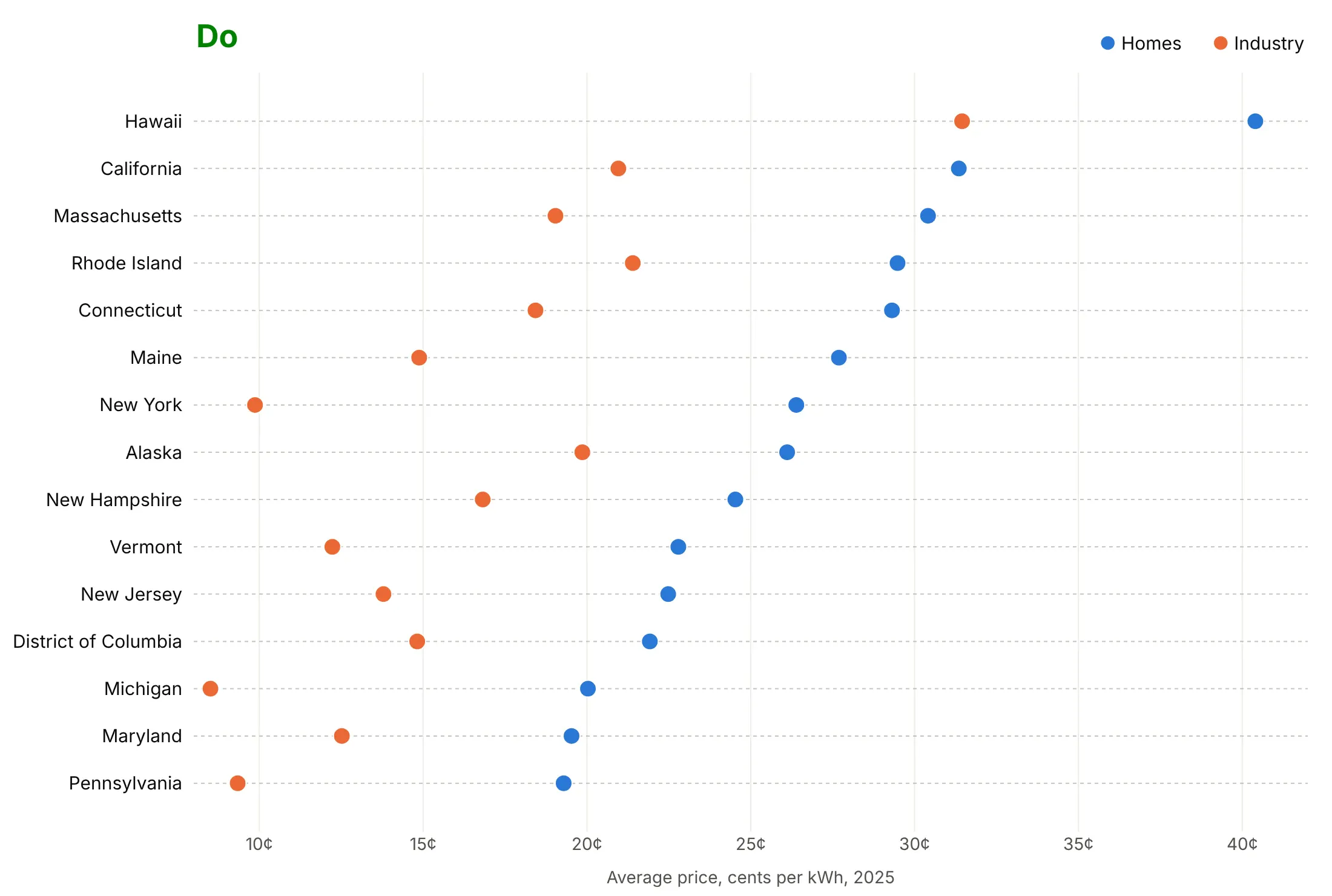
Here are the 15 highest home electricity prices in 2025, with the price for industry next to each, drawn both ways with the same colors.

Don't connect the dots with lines across rows, leave rows in alphabetical order, or publish raw column names and numbers without units. Lines between unrelated states suggest a trend that doesn't exist, and the alphabetical order hides the ranking:

Do sort the rows by a value, draw dots only, add light dotted guides across each row, and put the unit on the axis:

Choose what the order and color say

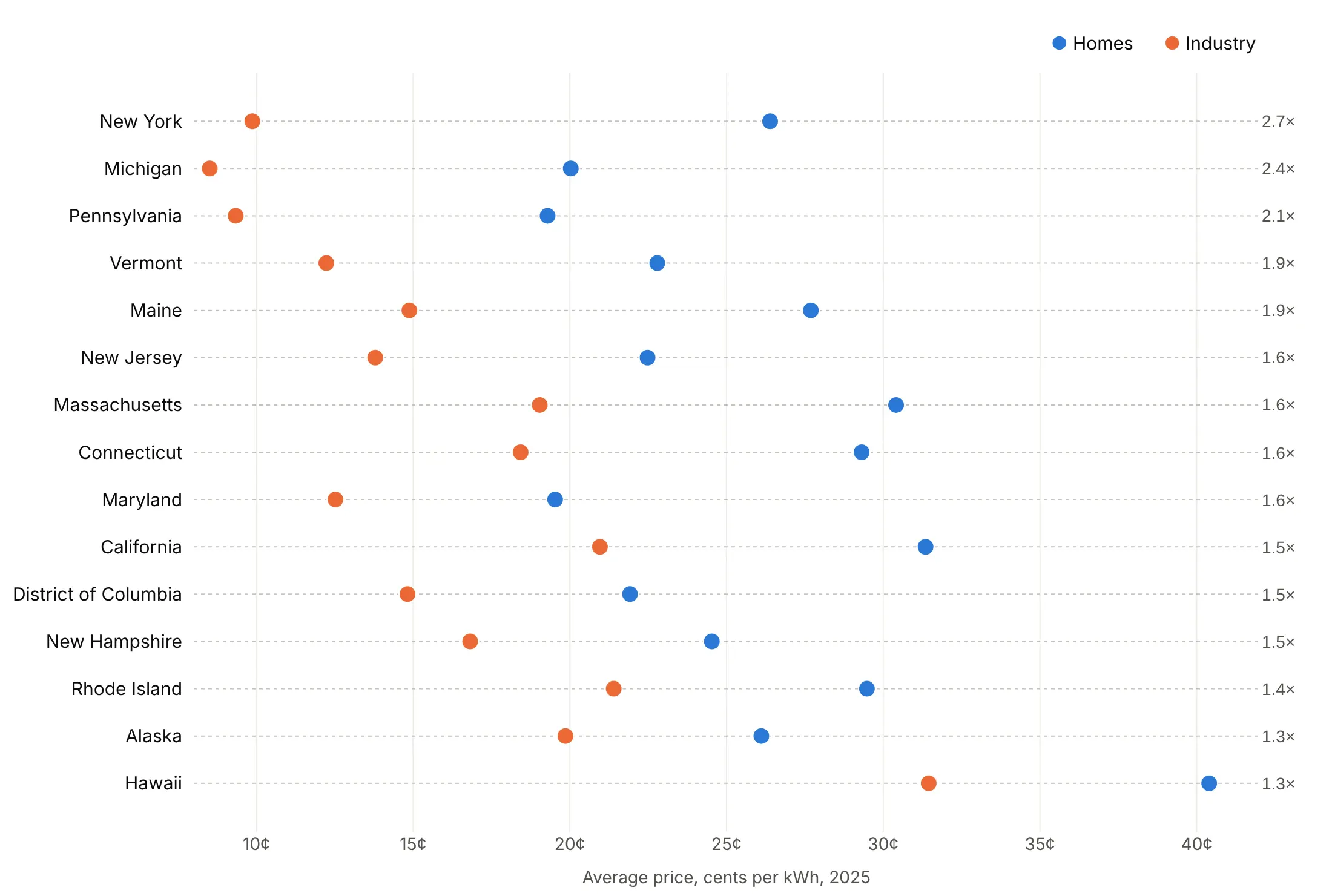
Sort by the gap when the gap is the story. Here the rows are sorted by the home price divided by the industry price, from 2.7 in New York to 1.3 in Hawaii, printed on the right.

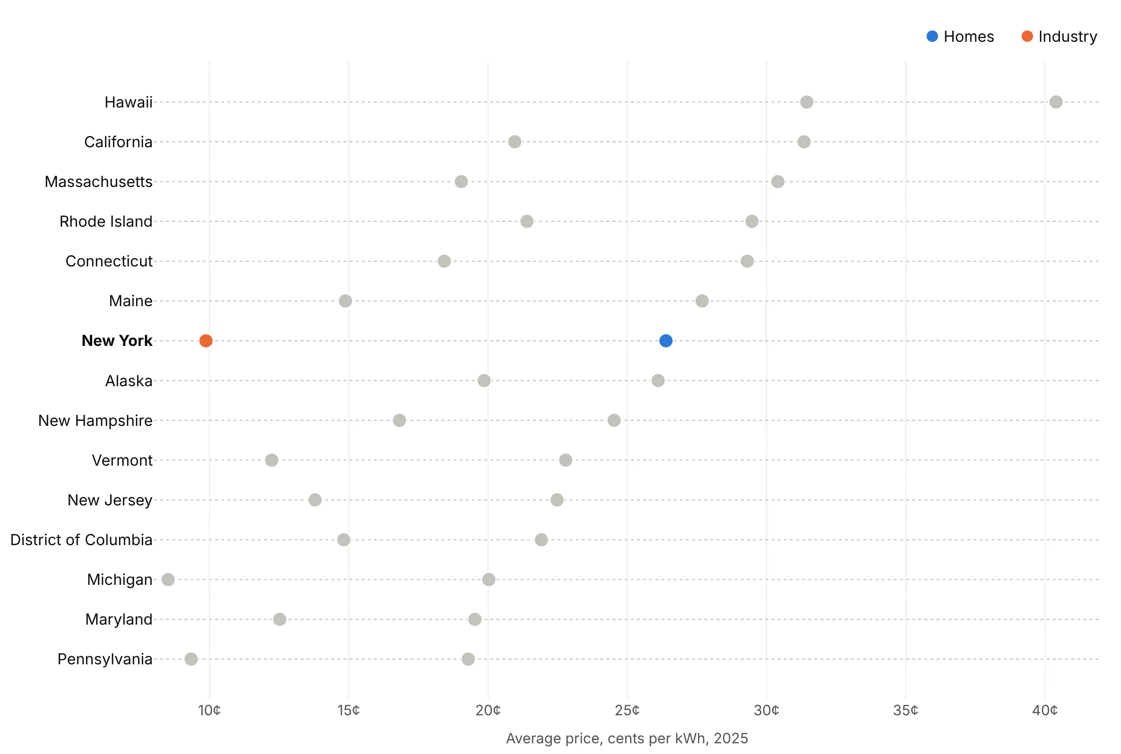
Highlight one row. Color New York and gray the rest when the chart is about one state.

Checklist

Do

• Sort the rows by the value that matters, unless they have a natural order.
• Use mode="markers" and one trace per series.
• Add dotted grid lines across the rows (yaxis.griddash="dot").
• Use a zoomed or log axis when it helps; a dot has no length to distort.
• Name the series in a legend or color key above the plot, in the order the dots appear.
• Write a title that states the takeaway with a number.

Don't

• Join dots in different rows with lines.
• Use more than about five series per row; split into panels instead.
• Let one outlier set the axis range; clip it and print its value.
• Use a dot plot for parts of a whole; use a stacked bar or a treemap.

Options to customize

These are the go.Scatter and layout options that matter for a dot plot. The full list is in the Plotly scatter reference.

1. mode="markers": dots without lines. Use "markers+text" to print values next to the dots.
2. x, y: the value on x and the category on y, one trace per series.
3. marker.size, marker.color: 10 to 15 px dots; one color per series, or a list for per-row colors.
4. marker.line: a 1 px white outline keeps overlapping dots apart.
5. marker.symbol: circle-open for a context series, arrow-right for a value drawn off the scale.
6. error_x with array, arrayminus, width=0: confidence intervals or ranges as thin lines.
7. yaxis.categoryorder="array", categoryarray: fixes the row order, sorted or natural.
8. yaxis.showgrid, gridcolor, griddash="dot": the dotted row guides.
9. xaxis.type="log": a log axis for values that span orders of magnitude.
10. xaxis.range: zoom in or clip outliers; a dot plot doesn't need zero.
11. fig.add_vline: a target, a median or a regulatory minimum.
12. make_subplots(rows, cols, shared_xaxes=True): panels by group, or two columns for 50 rows.
13. customdata, hovertemplate: units and extra columns on hover.
14. go.Scattergl: WebGL markers for tens of thousands of dots.

More dot plot examples

Eight more dot plots built from real public data, each with its source, the technique that makes it work and a prompt to rebuild it.

1. The cost of new renewable power since 2010

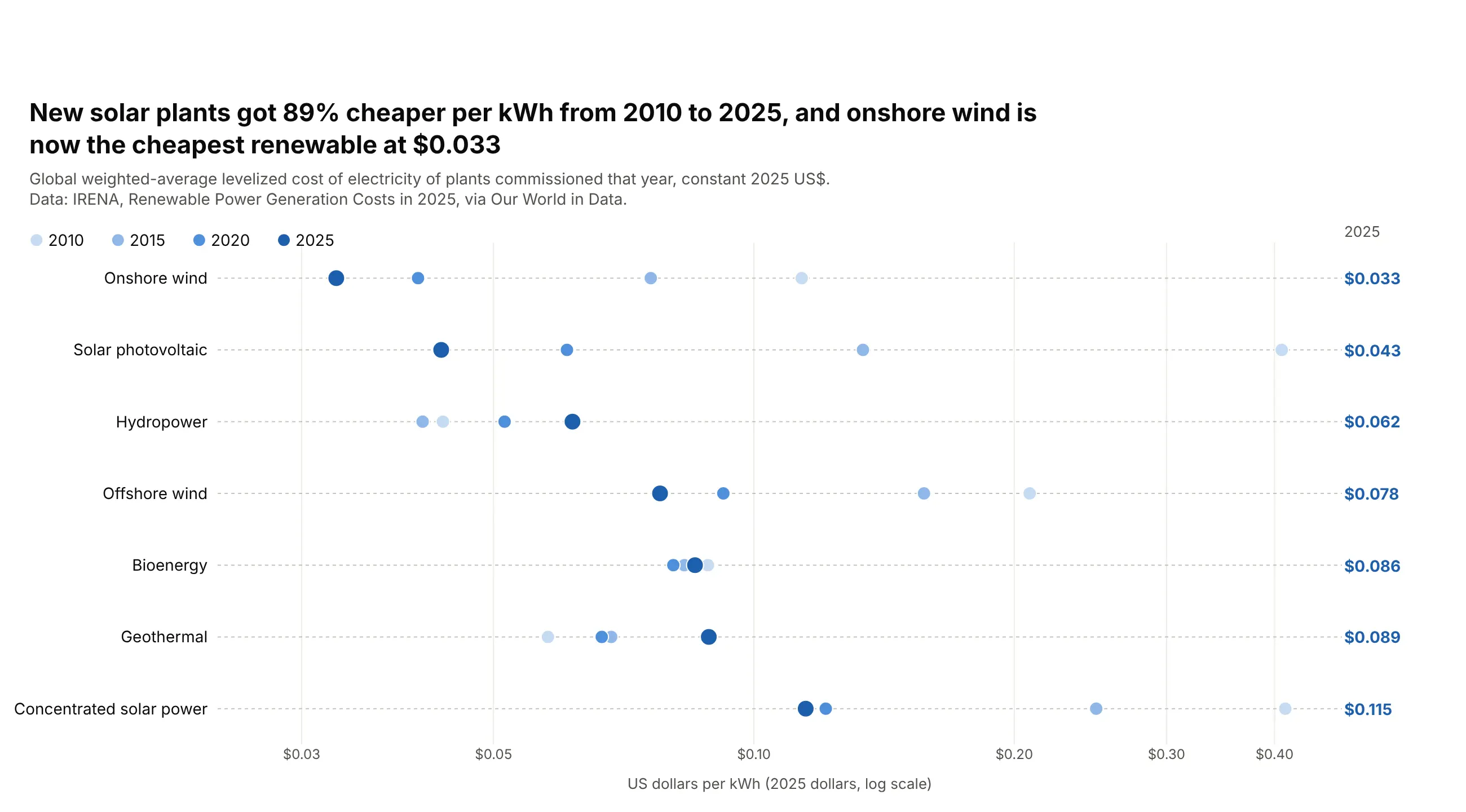
Electricity from new solar plants cost 89% less in 2025 than in 2010, at $0.043 per kWh, and onshore wind was cheapest at $0.033. Hydropower and geothermal got more expensive. Data: IRENA, Renewable Power Generation Costs in 2025, via Our World in Data.

Tip: a log axis shows the 2010 values and the 2025 values in one chart, and only dots, not bars, can use one.

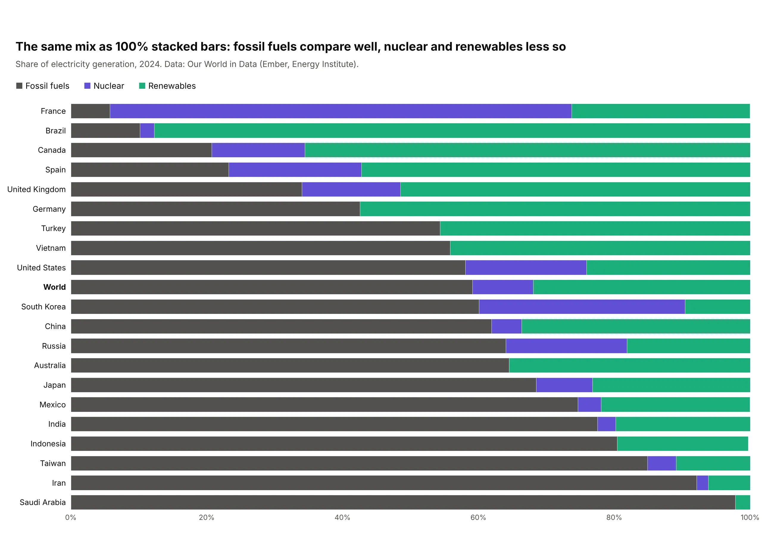
2. Where electricity comes from in 20 countries

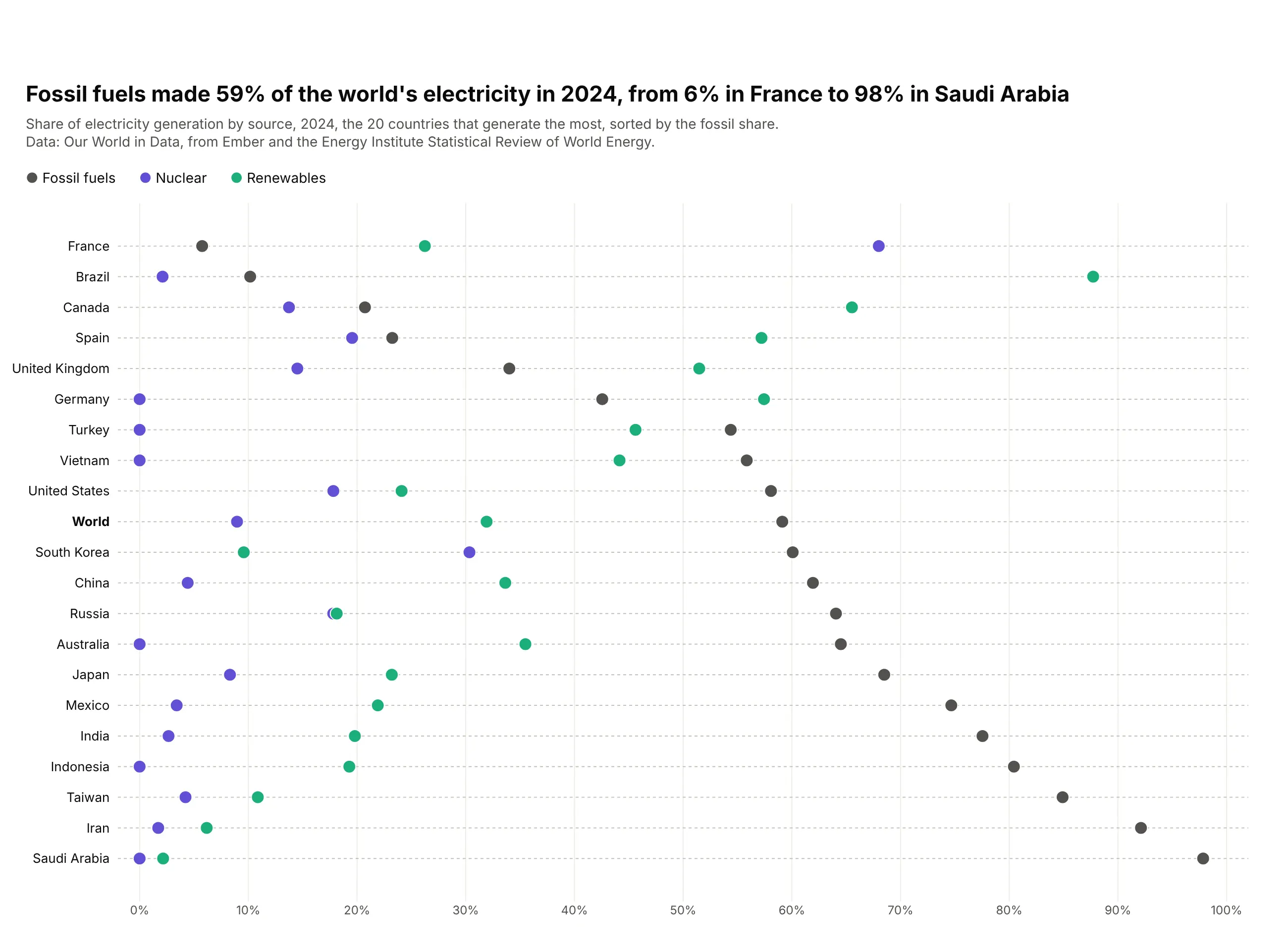
Fossil fuels made 59% of the world's electricity in 2024, from 6% in France, where nuclear made 68%, to 98% in Saudi Arabia. Brazil got 88% from renewables. Data: Our World in Data, from Ember and the Energy Institute.

Tip: fix the axis at 0 to 100% so every share is read against the same whole.

Another way to see it: 100% stacked bars show that each row adds up to the whole, but only the fossil segment starts at a common baseline, so nuclear and renewables are harder to compare.

3. Bank capital in the Fed's 2026 stress test

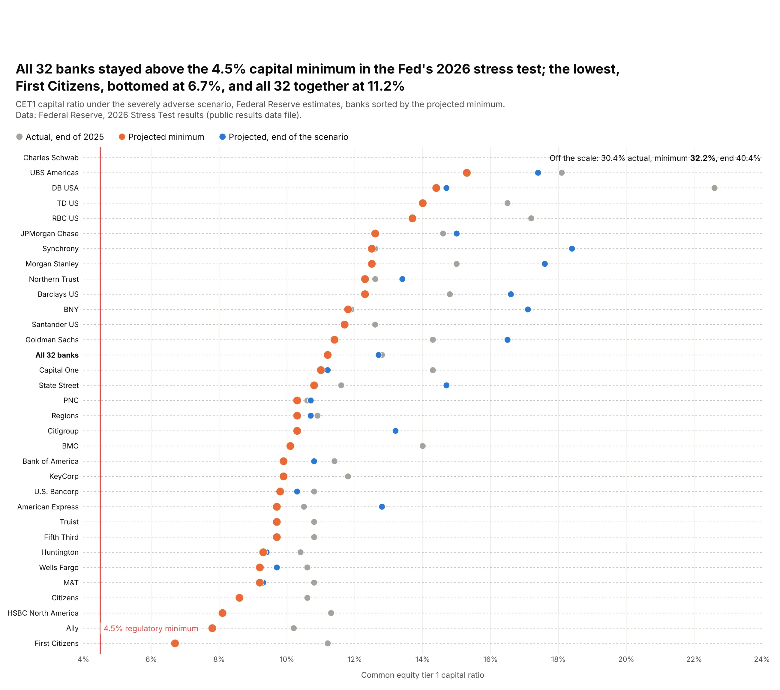
All 32 banks stayed above the 4.5% minimum capital ratio in the Fed's 2026 stress test. First Citizens had the lowest projected minimum at 6.7%, and the 32 banks together fell from 12.8% to 11.2%. Data: Federal Reserve, 2026 Stress Test results.

Tip: sort by the series that answers the question, here the low point, and draw the threshold as a line.

4. Returns of 14 asset classes over three horizons

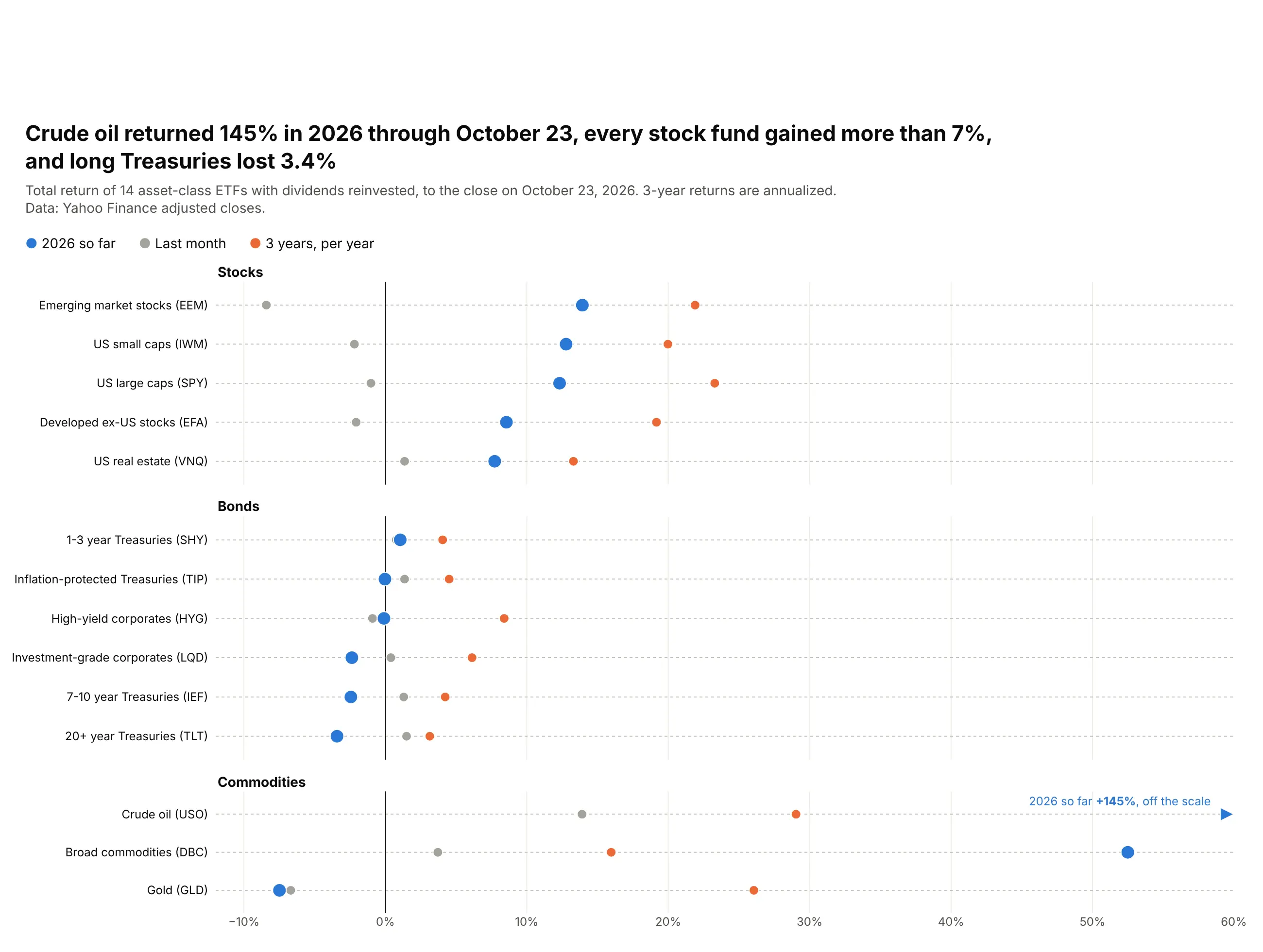
Crude oil returned 145% in 2026 through October 23, every stock fund gained more than 7%, and long Treasuries lost 3.4%. Gold fell 7.5% this year while returning 26% a year over three years. Data: Yahoo Finance adjusted closes.

Tip: split the rows into panels by asset class and draw a zero line, so gains and losses read at a glance.

5. What countries spend on retail drugs, and who pays

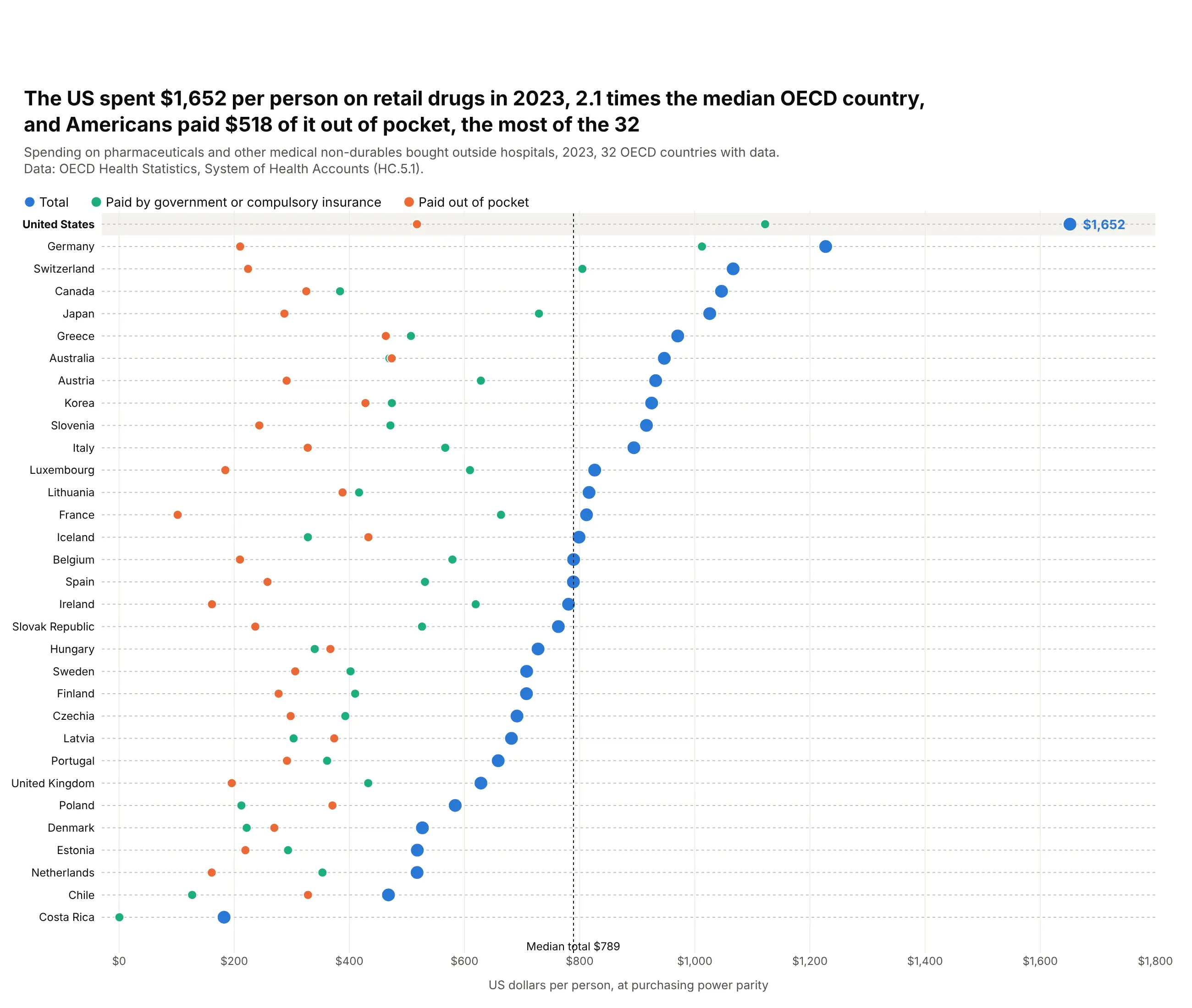
The US spent $1,652 per person on drugs bought outside hospitals in 2023, 2.1 times the median of the 32 OECD countries with data. Americans paid $518 of it out of pocket, the most of the 32. Data: OECD Health Statistics, System of Health Accounts.

Tip: make the total the big dot and its parts smaller, and shade the row the chart is about.

6. Hospital readmissions, hospital by hospital

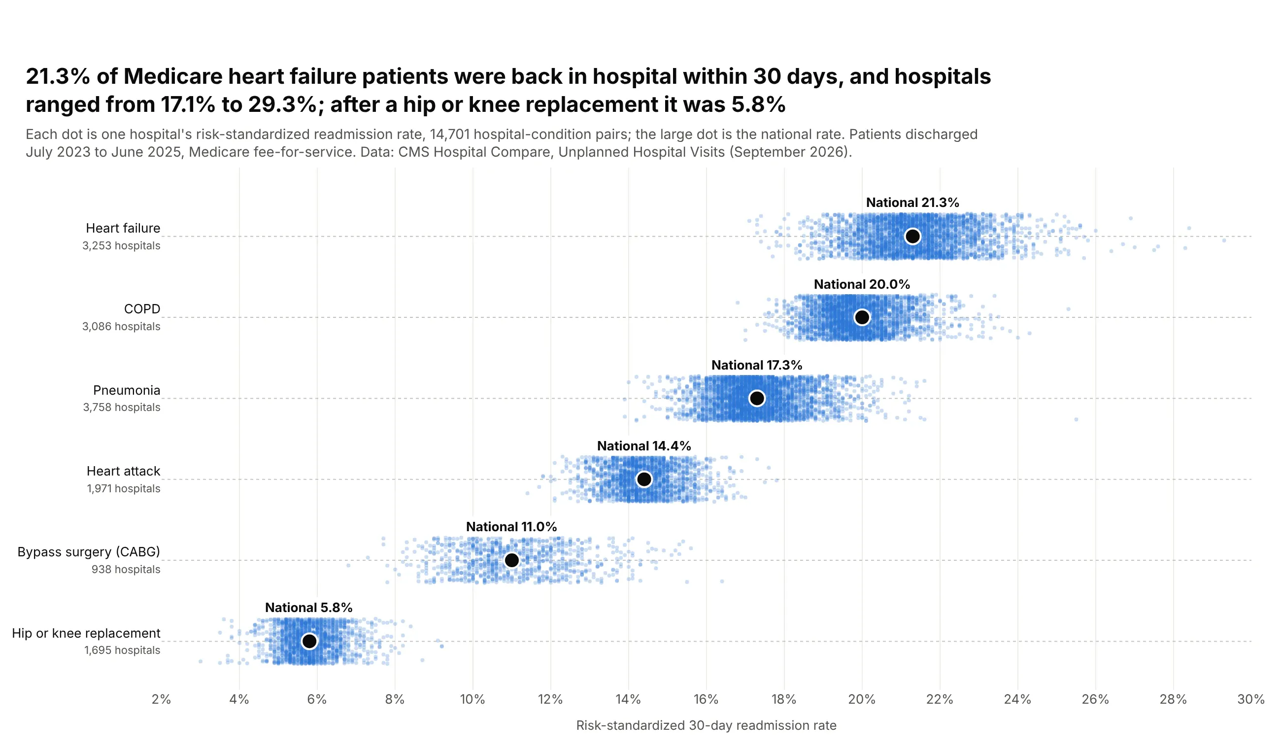
21.3% of Medicare heart failure patients were back in hospital within 30 days, and hospitals ranged from 17.1% to 29.3%. After a hip or knee replacement the national rate was 5.8%. Data: CMS Hospital Compare, Unplanned Hospital Visits.

Tip: with thousands of dots per row, make them small and translucent and jitter them vertically, then mark the summary with one large dot.

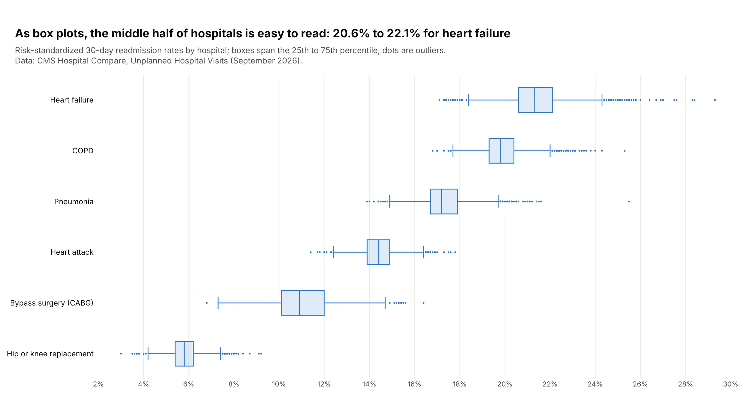
Another way to see it: box plots summarize the same hospitals and make the middle half easy to read (20.6% to 22.1% for heart failure), but they hide how many hospitals sit in each row.

7. How men and women spend their day

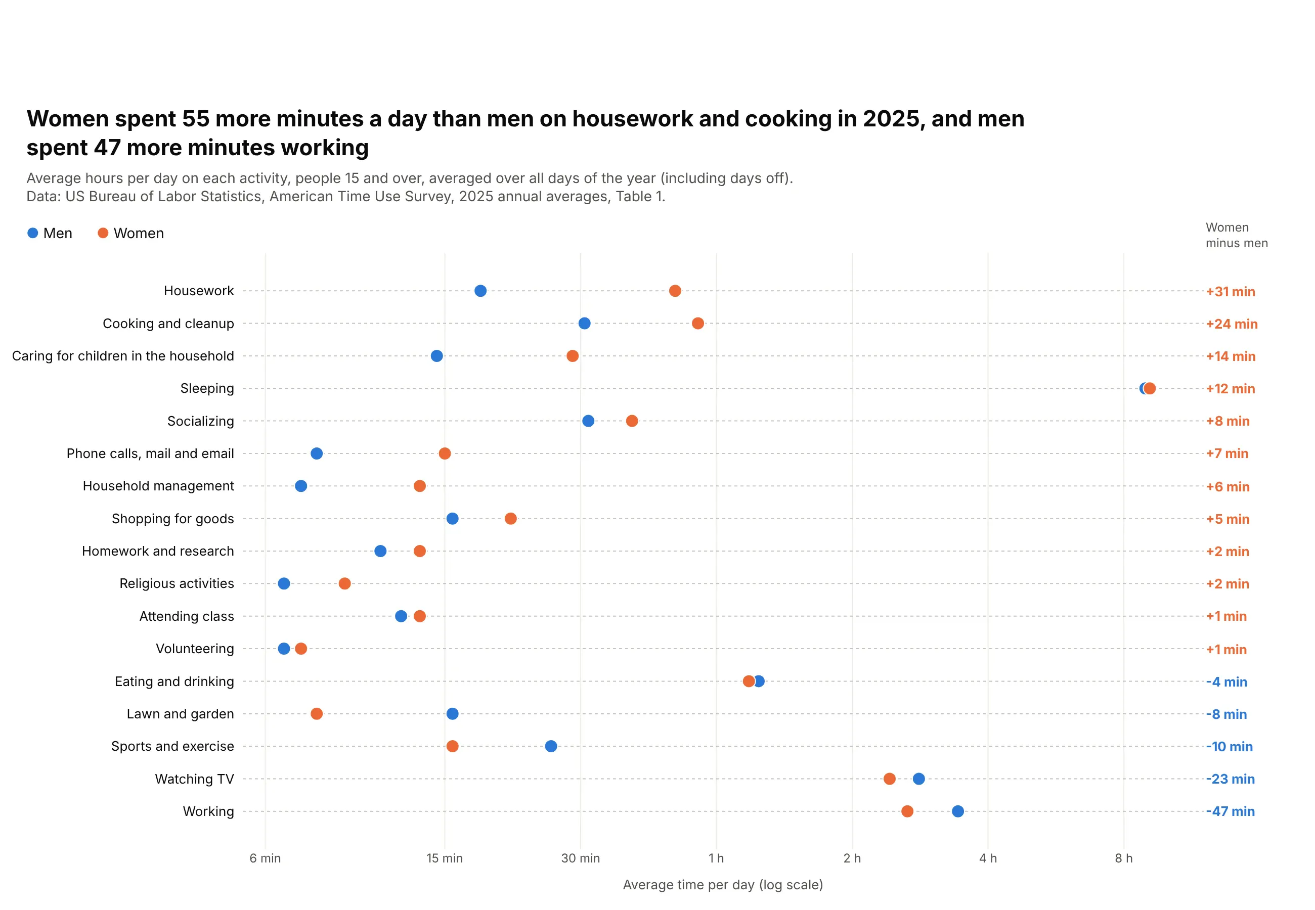
Women spent 55 more minutes a day than men on housework and cooking in 2025, and men spent 47 more minutes working. The averages include days off, so they are lower than a typical workday. Data: BLS, American Time Use Survey 2025.

Tip: sort by the difference and print it in a column, so the chart reads like a table with a picture.

8. The size of plotly.js bundles

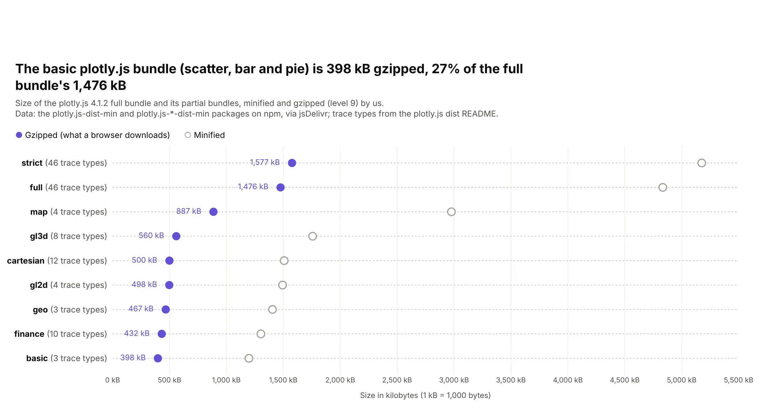
The basic plotly.js bundle, with scatter, bar and pie charts, is 398 kB gzipped, 27% of the full bundle's 1,476 kB. Gzip shrinks every bundle about three times. Data: plotly.js 4.1.2 on npm, gzipped by us.

Tip: use a hollow dot for the secondary series so the one that matters stands out.