Small Multiples - A Complete Guide (with 13 Examples)

TL;DR

• Small multiples repeat the same small chart once per group, with the same axes and encoding, so the eye compares panels instead of untangling lines.
• Small multiples are also known as trellis charts, lattice charts, panel charts and facet plots, and are similar to ridgeline plots and scatter plot matrices.
• Use them when one chart would hold more than about five overlapping series, or when each group needs its own reference band, map position or distribution.
• Share the axes unless the sizes differ so much that the small groups go flat, then label every panel's scale, index each series to a common base, or draw every other group in gray behind each panel.
• In Python, px.line(df, x=..., y=..., facet_col="group", facet_col_wrap=4) makes one in one line of code, and make_subplots handles custom grids such as a map of US states.

What is a small multiple chart?

Small multiples look like this:

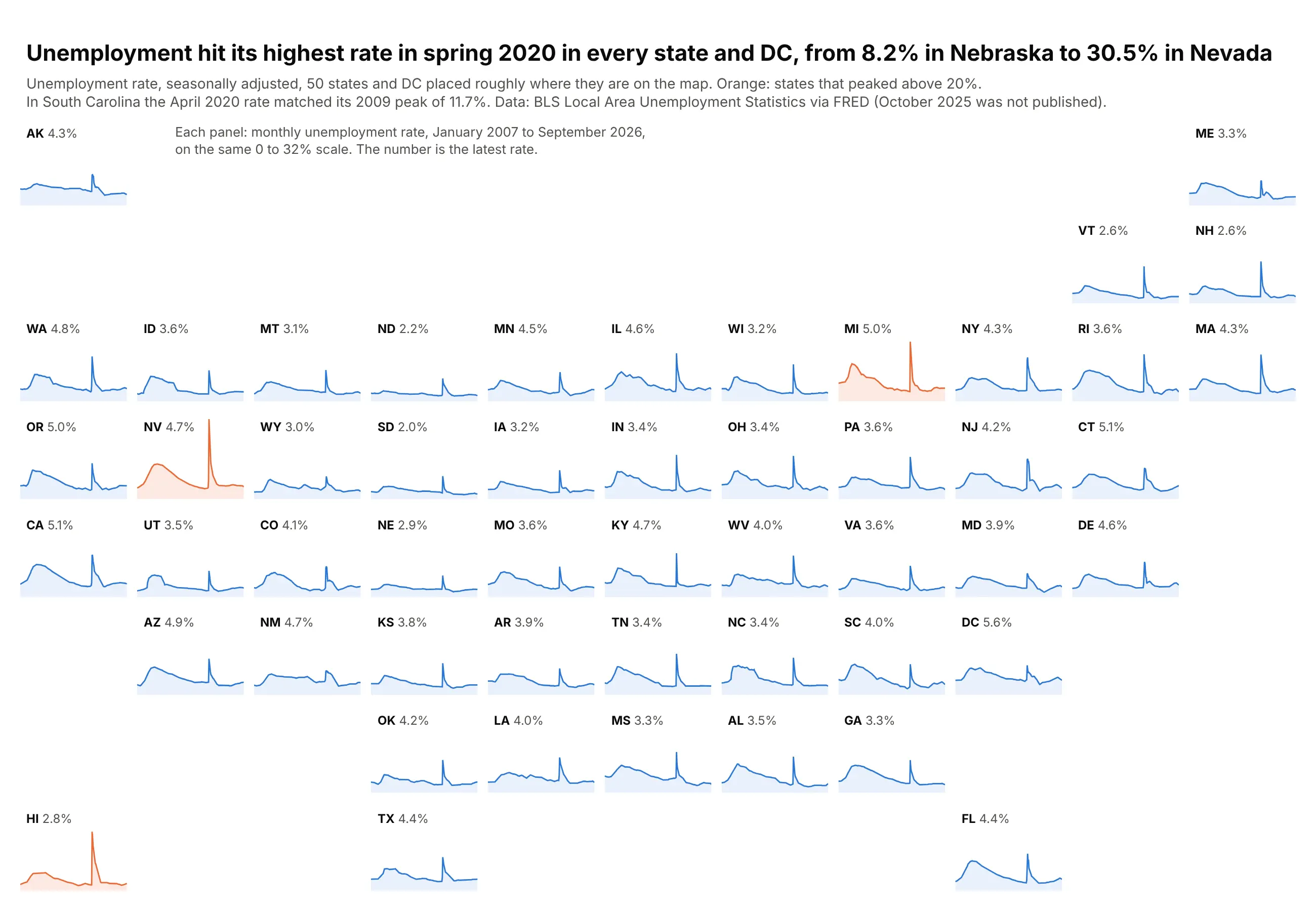
Data: BLS Local Area Unemployment Statistics via FRED.

How do you read small multiples? In the example above, notice these things:

• Each panel is the same small area chart, one state's monthly unemployment rate, and the panels sit roughly where the states are on a US map, so Alaska is in the top left and Maine in the top right.
• Every panel shares the same time axis and the same 0 to 32% scale, so a taller line means a higher rate and you can compare any two states by eye without reading their axes.
• Because the panels repeat one design, the eye picks up the shared shape first. Almost every state has a wide hump during the Great Recession and a sharp spike in spring 2020, so a state that breaks the pattern stands out, like South Carolina, whose earlier hump reached the same 11.7% as its pandemic spike.
• Color picks out the panels worth a second look. Nevada, Michigan and Hawaii are orange because their peaks went above 20%, and the number next to each state's name is its latest rate.
• The shared scale has a cost, since states with low rates such as North Dakota and South Dakota draw nearly flat lines whose small changes are hard to see. Switch to independent y axes when the shape within each state matters more than the comparison between them.

It's often used for charts like these:

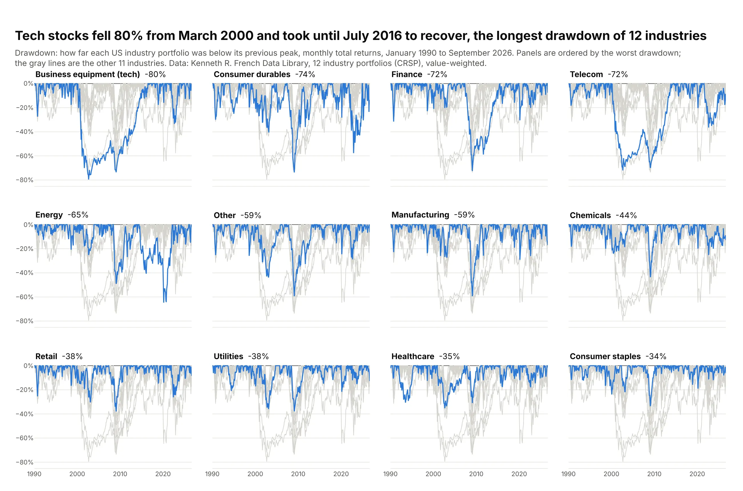
Highlighting one series against all the others. Tech stocks fell 80% from March 2000 and took until July 2016 to recover, the longest drawdown of 12 US industries since 1990. Data: Kenneth R. French Data Library (CRSP).

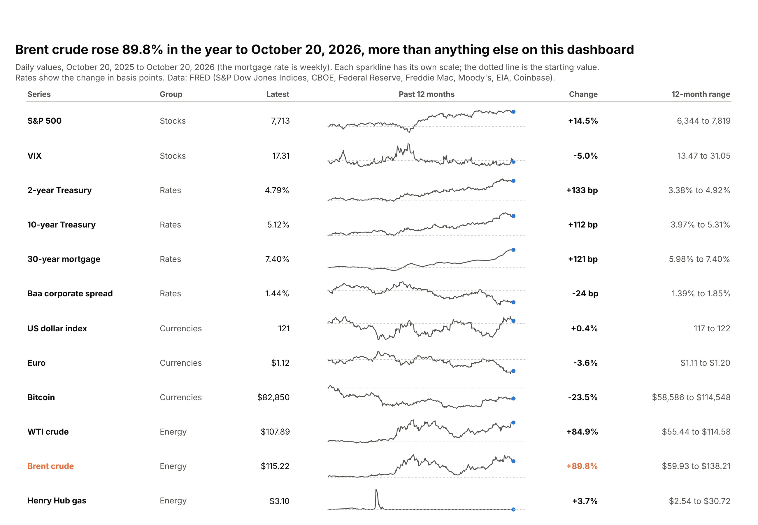
Sparklines in a table. Brent crude rose 89.8% in the year to October 20, 2026, more than any other series on a 12-row market dashboard. Data: FRED.

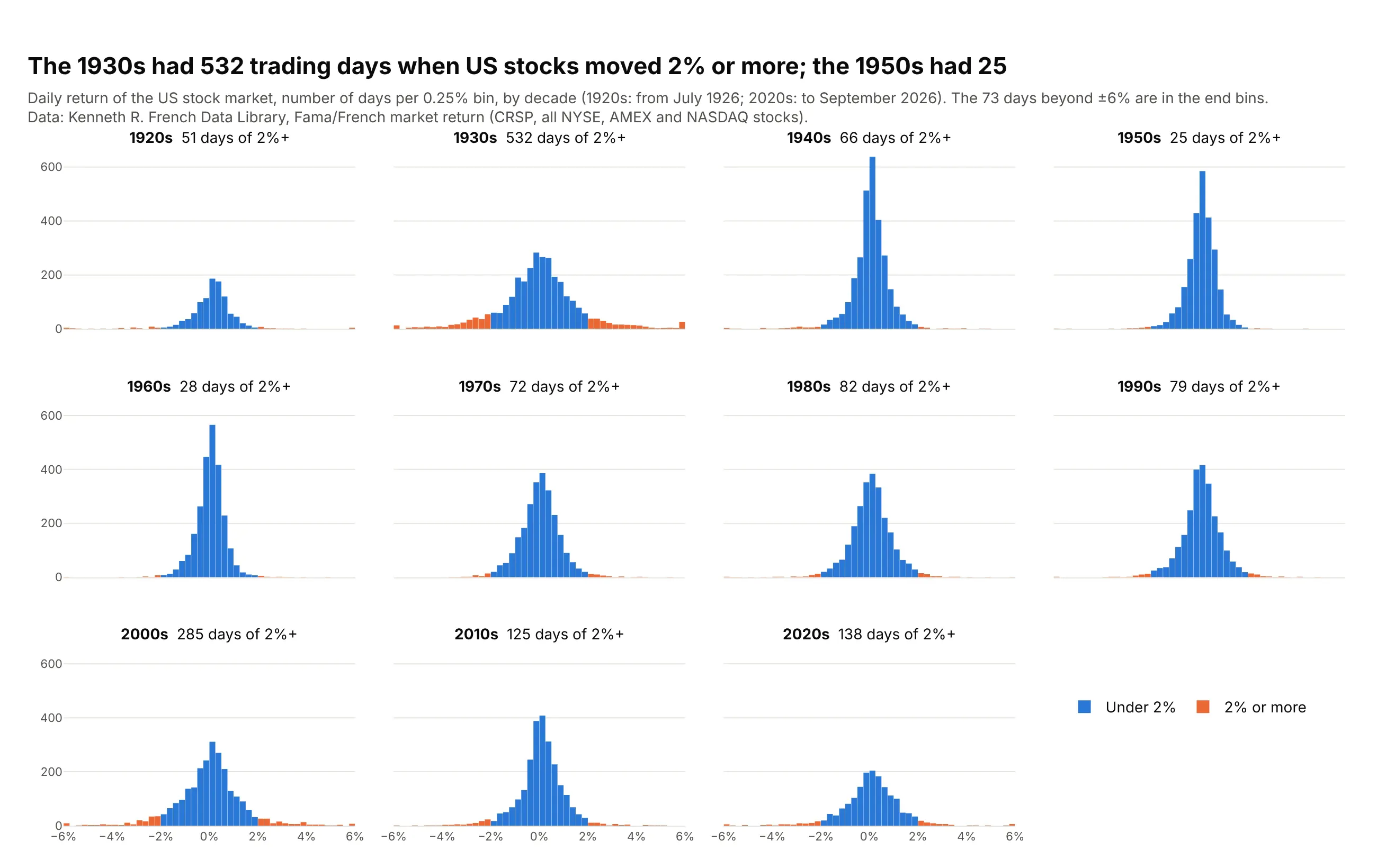
Distributions by group. The 1930s had 532 trading days when US stocks moved 2% or more, and the 1950s had 25. Data: Kenneth R. French Data Library (CRSP).

A short history

Edward Tufte named and popularized small multiples in The Visual Display of Quantitative Information (1983). William Cleveland and colleagues at Bell Labs turned them into the trellis display, a grid of panels conditioned on one or two variables (Becker, Cleveland and Shyu, 1996). Cleveland's best-known example, in Visualizing Data (1993), used barley yields from six Minnesota sites (Immer, Hayes and Powers, 1934):

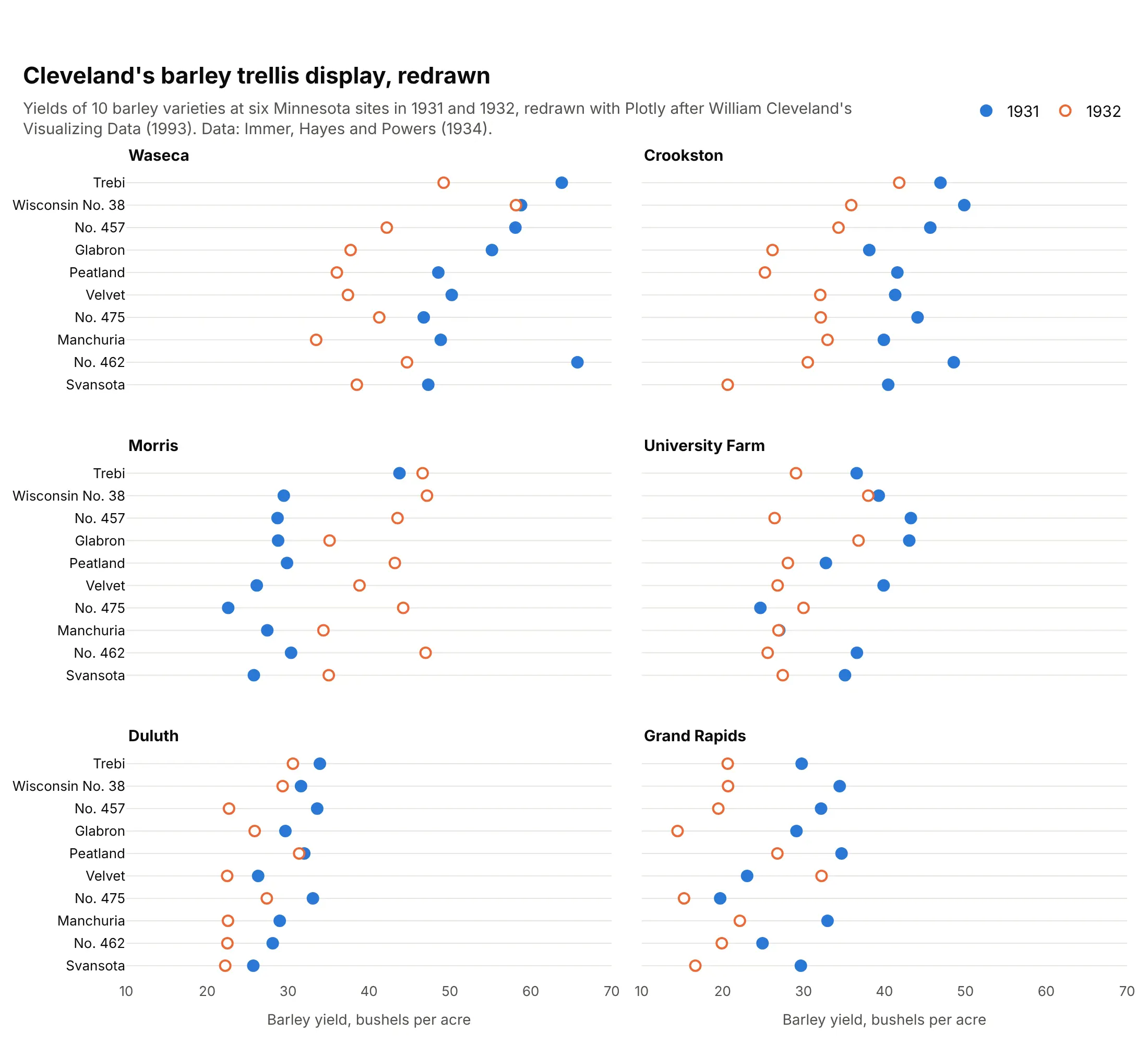
At Morris all 10 varieties yielded more in 1932 than in 1931, while at the other five sites at most one did. Laid out in panels, the exception is obvious, and Cleveland suggested the two years may have been swapped in the records.

Alternatives to small multiples

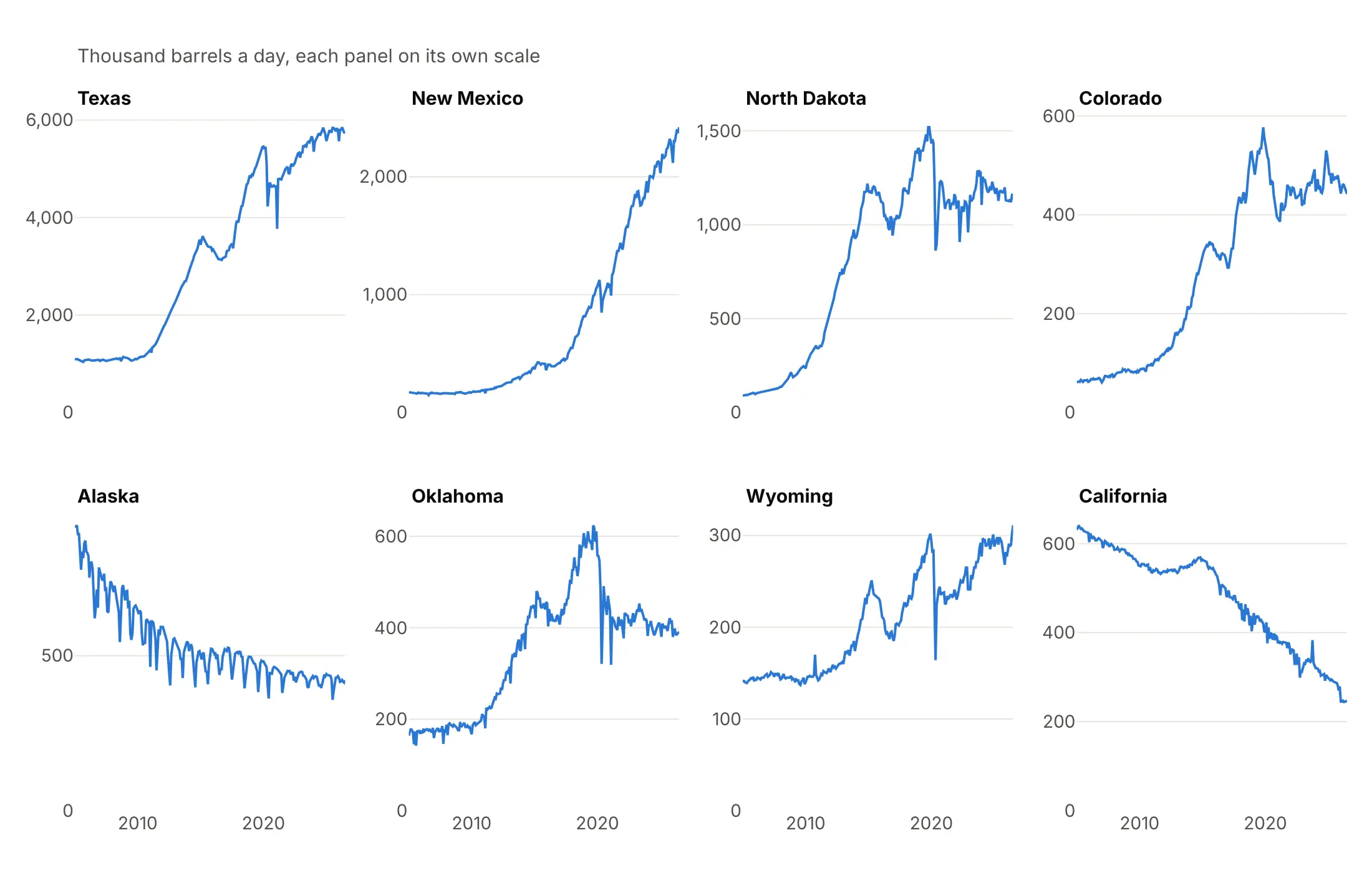
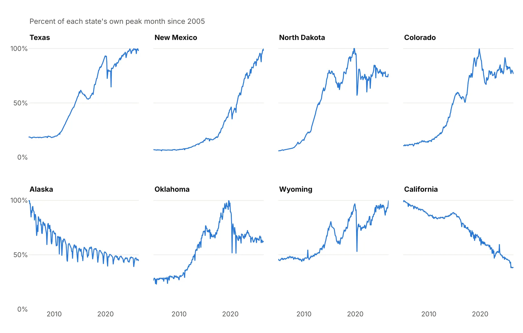
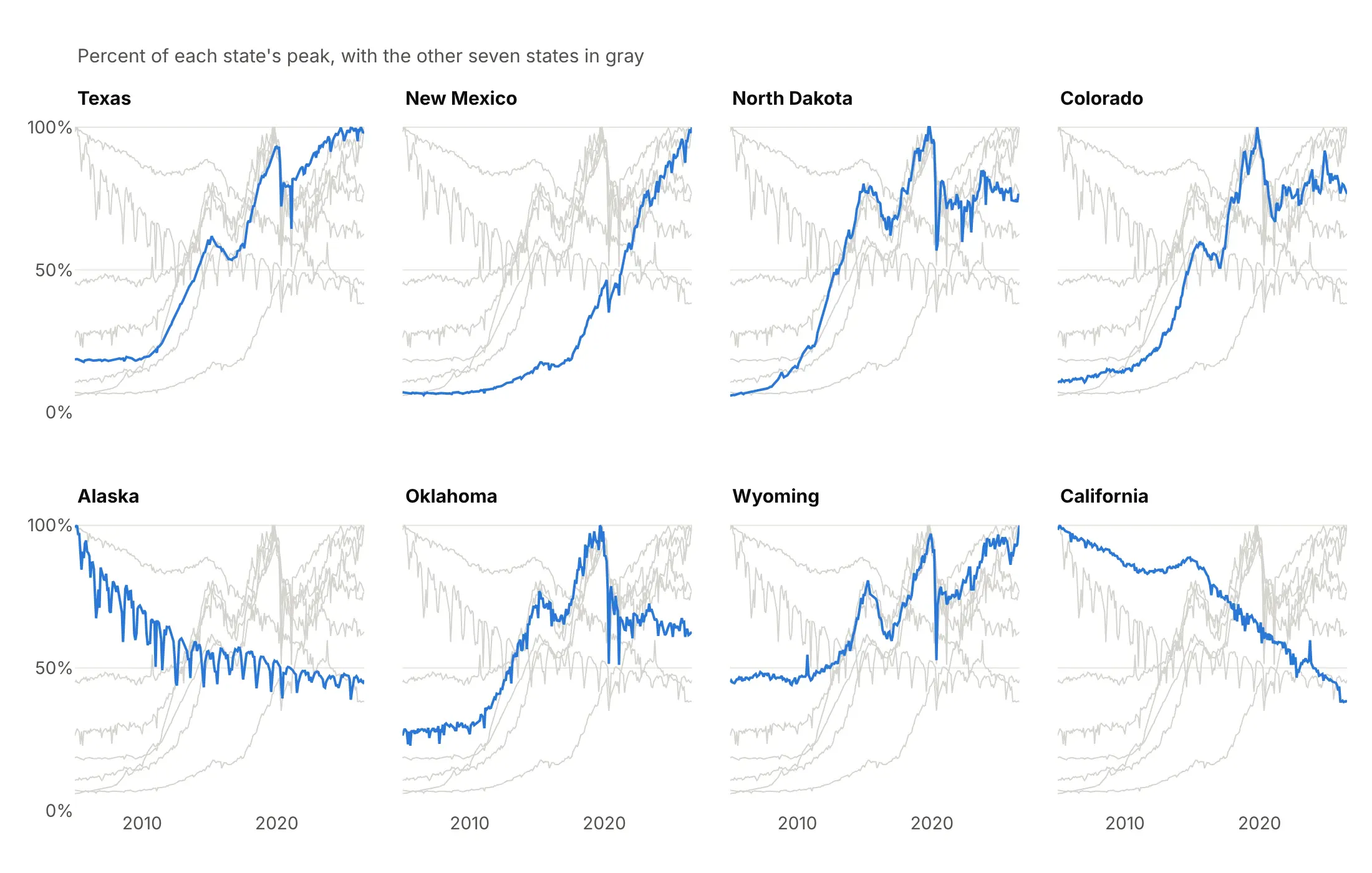
Here's the same monthly crude oil production of eight states drawn four ways. Some are better for the question, some worse, some just different:

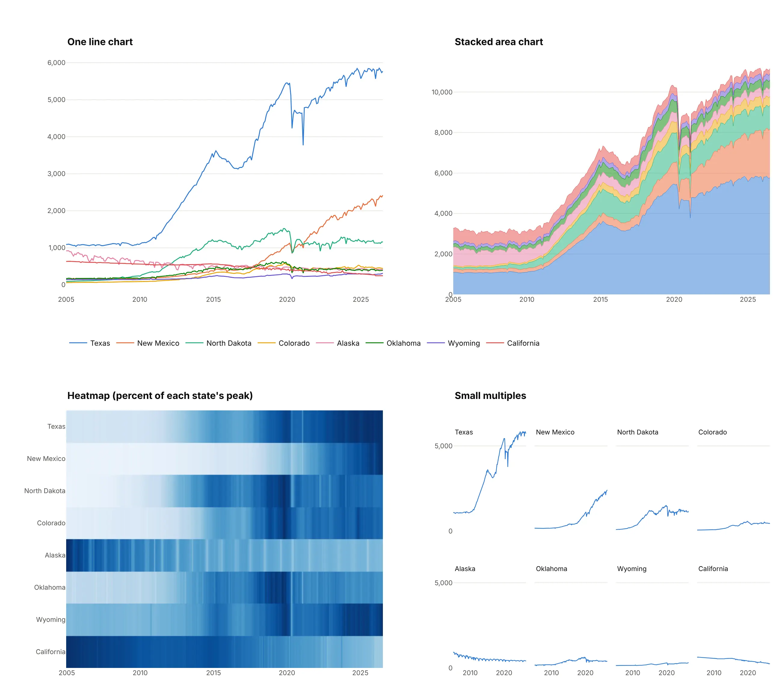
• One line chart (works too, for a few series). Up to four or five lines it is the most compact choice. With eight states, the five smaller ones overlap below 1,000 thousand barrels a day and the colors become a legend lookup.
• Stacked area chart (different). Shows the total, about 11 million barrels a day for these eight states, but only the bottom band has a flat baseline, so the other states' trends are hard to read.
• Heatmap (better for many series and timing). Scaled to each state's peak, it shows when each state grew in one compact block, and it fits hundreds of rows. Color is less precise than position, so exact values are hard to read. See our heatmap guide.
• Small multiples (better for comparing shapes). Each state's line is readable on its own and comparable with the others on the shared axis. They take more room, and you lose the exact overlap of two series in one panel.

For distributions by group, a ridgeline plot is a compact alternative to faceted histograms (see our ridgeline plot guide), and a scatter plot matrix is small multiples of every pair of variables (see our scatter plot matrix guide).

How to make small multiples

With AI

ChatGPT, Claude Code, GitHub Copilot, Cursor and other AI tools are excellent at writing Plotly code. Name Plotly in the prompt, say what one panel shows, how to lay out and order the panels and whether the axes are shared:

With Plotly Studio

Plotly Studio is a desktop app where you point an AI at a dataset and it builds charts and a Dash app around your questions. Ask for small multiples the same way:

Show the weekly flu hospitalization rate for every state as a grid of small area charts, sorted by each state's peak, with the national rate as a dotted gray line in every panel. Add a dropdown to switch between flu, COVID-19 and RSV.

Make small multiples in Python or JavaScript

This is the code AI tools write under the hood. In Python, Plotly Express makes a faceted chart from a long table with one row per point:

Plotly Express and make_subplots both build small multiples as a grid of ordinary subplots, one pair of axes per panel. For layouts px can't make, this helper places each panel at a grid position (a map of states, as in the first chart on this page) and can draw every other group in gray behind each panel:

In JavaScript, plotly.js puts each trace on its own xaxis/yaxis pair, layout.grid lays the pairs out, and matches shares an axis:

Share it

Every Plotly chart has a Share chart button (the cloud icon in its toolbar) that uploads it to Plotly Cloud and gives you a link. Only you can see it until you change its visibility.

For a live app, put the chart in a Dash app and publish it with the Plotly Cloud CLI. Coding agents can run these commands for you:

If your data has to stay in your own cloud or data center, publish to Dash Enterprise instead.

Dos and don'ts

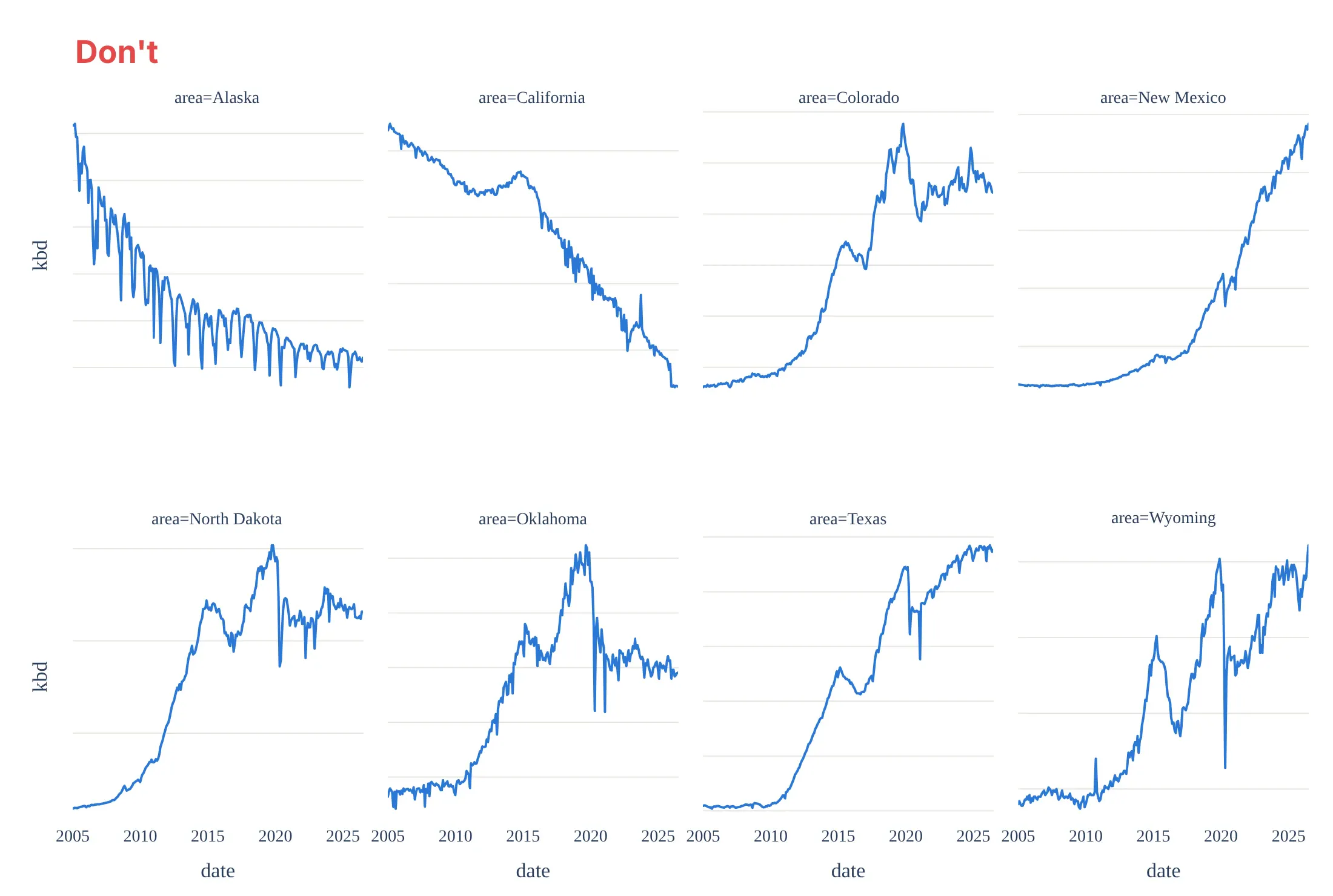
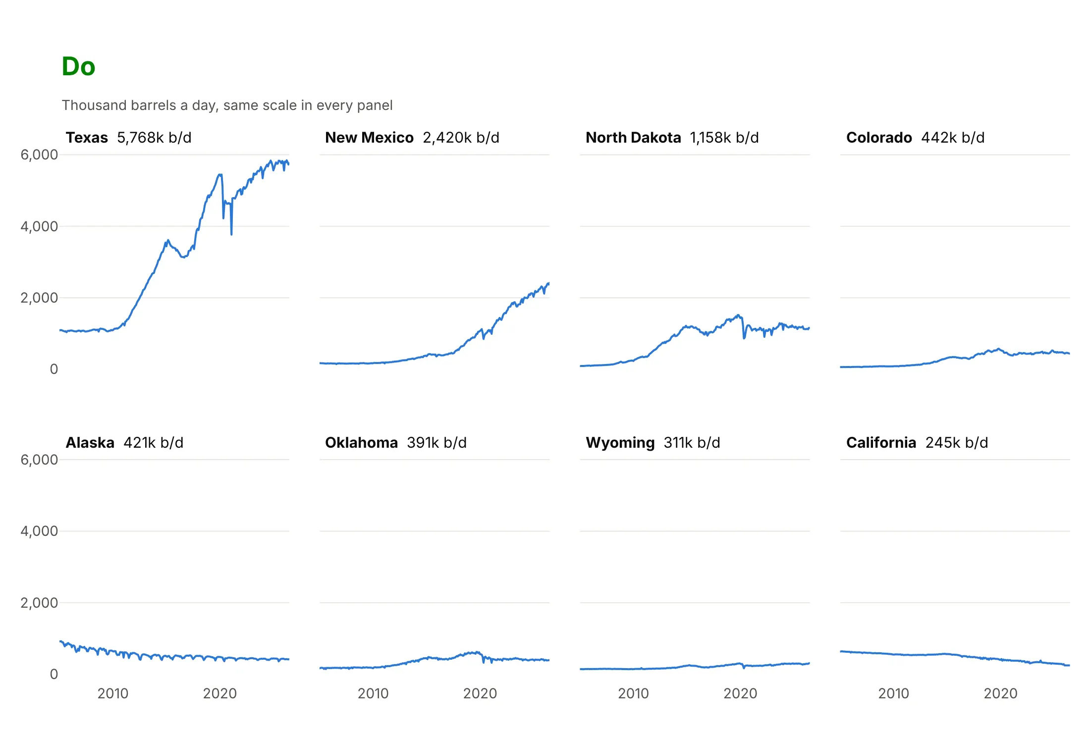
Plotly Express gives you a working grid in one line, and most of the work for a published chart is in the axes, the order and the panel labels. Here is the crude oil production of eight states both ways, with the same color.

Don't hide the scales of independent y axes, sort the panels alphabetically, keep the "area=" prefixes or repeat the axis titles under every panel:

Do share and label the y axis, order the panels by size, and put the name and the latest value in each panel title:

Shared, independent or indexed axes

The axis choice decides what the panels compare. Here are four options on the same data.

Shared axes. Panels compare sizes, and it's the right default. Texas dwarfs everything, so the small states look flat.

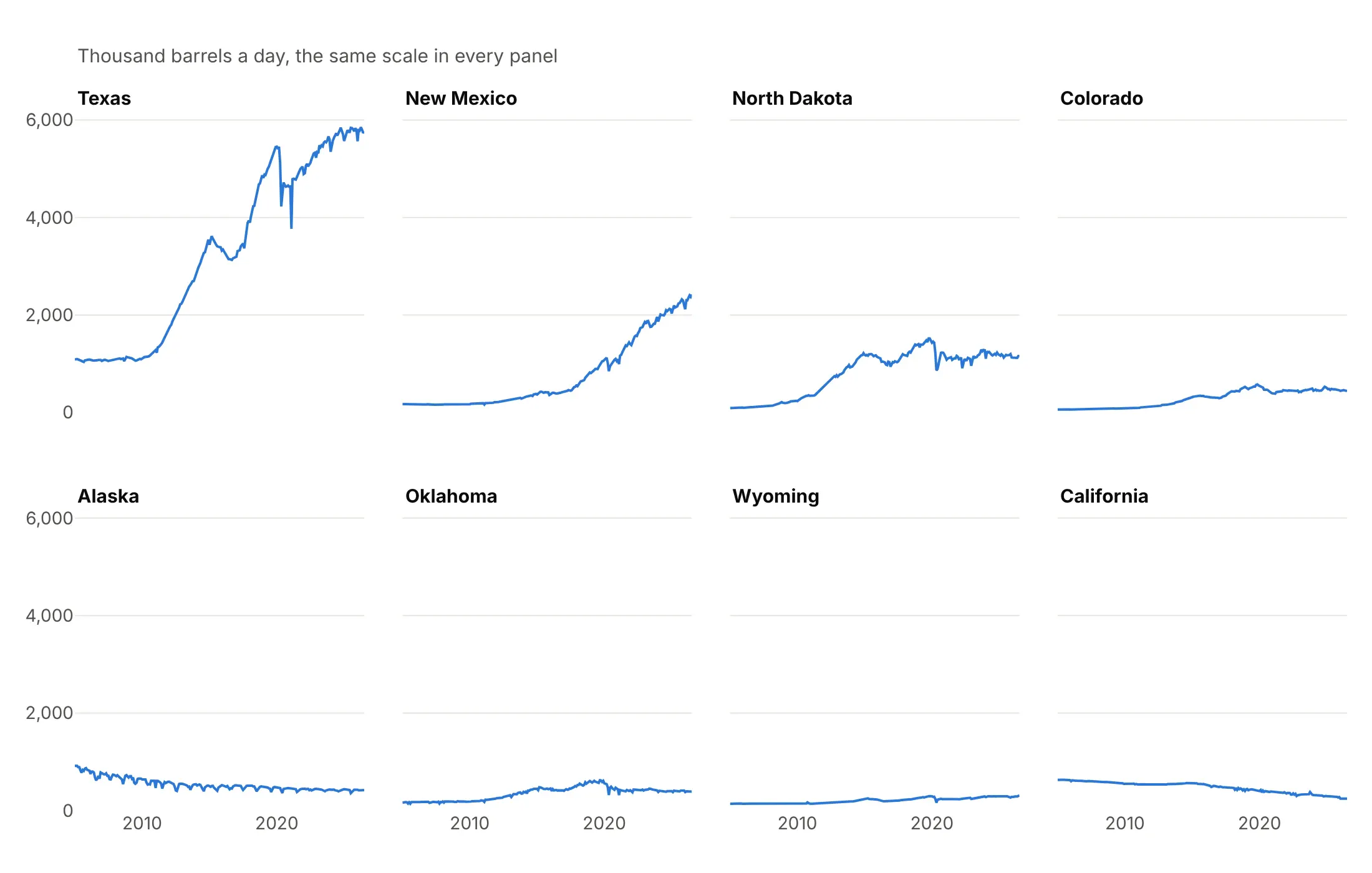
Independent axes. Every shape is readable, but panels no longer compare by height, so every panel needs its own labeled scale. In Plotly Express, use fig.update_yaxes(matches=None, showticklabels=True).

Indexed to a common base. Each state as a percent of its own peak shares one axis again and compares timing: New Mexico and Wyoming are at their peaks now, Texas is 1% below its peak, North Dakota peaked in 2019 and Alaska in 2005.

Indexed, with the others in gray. Adds every other state behind each panel, so you can see whether a state is typical or an outlier.

Checklist

Do

• Write a title that states the takeaway, and put the panel's key number in each panel title.
• Share the axes by default, and say so when they aren't shared.
• Order the panels by something meaningful: size, peak, change or geography.
• Label each axis once, and show tick labels only on the outer panels.
• Use one color for the main series, and save other colors for a highlight.

Don't

• Hide the scale of independent axes.
• Leave "column=value" in the panel titles.
• Sort panels alphabetically when the ranking matters.
• Add a legend for something the panel titles already say.
• Make panels so small that the lines can't show a shape.

Options to customize

These are the Plotly Express and make_subplots options that matter most for small multiples. The full lists are in the Plotly facet plots documentation and the subplots documentation.

1. facet_col, facet_row (px): one column or row of panels per value of a column; use both for a grid of two variables.
2. facet_col_wrap (px): wraps a single facet variable into rows of N panels.
3. category_orders (px): the panel order, for example {"state": ["Texas", "New Mexico", ...]} sorted by size.
4. facet_col_spacing, facet_row_spacing (px): gaps between panels, as a fraction of the figure; lower them for big grids.
5. fig.for_each_annotation(...): rewrites the panel titles, for example to drop the "column=" prefix.
6. fig.update_yaxes(matches=None): gives every panel its own y range; add showticklabels=True so each scale is labeled.
7. make_subplots(rows, cols): the grid for custom layouts; place each trace with row= and col=.
8. shared_xaxes, shared_yaxes: True shares within a row or column, "all" across the whole grid.
9. subplot_titles: one title per grid cell, in row order, with "" for empty cells.
10. horizontal_spacing, vertical_spacing: gaps between make_subplots panels.
11. specs: cells that span several columns or rows, or that hold a map, a table or a polar chart.
12. row="all", col="all": add the same reference line or shape to every panel with add_hline or add_shape.
13. xref="x2 domain": places an annotation relative to one panel, for labels inside the panel.
14. layout.grid (plotly.js): lays out axis pairs in rows and columns without Python.

More small multiple examples

Nine more small multiples built from real public data, each with its source, the technique that makes it work and a prompt to rebuild it.

1. Daily electricity demand for seven US grids

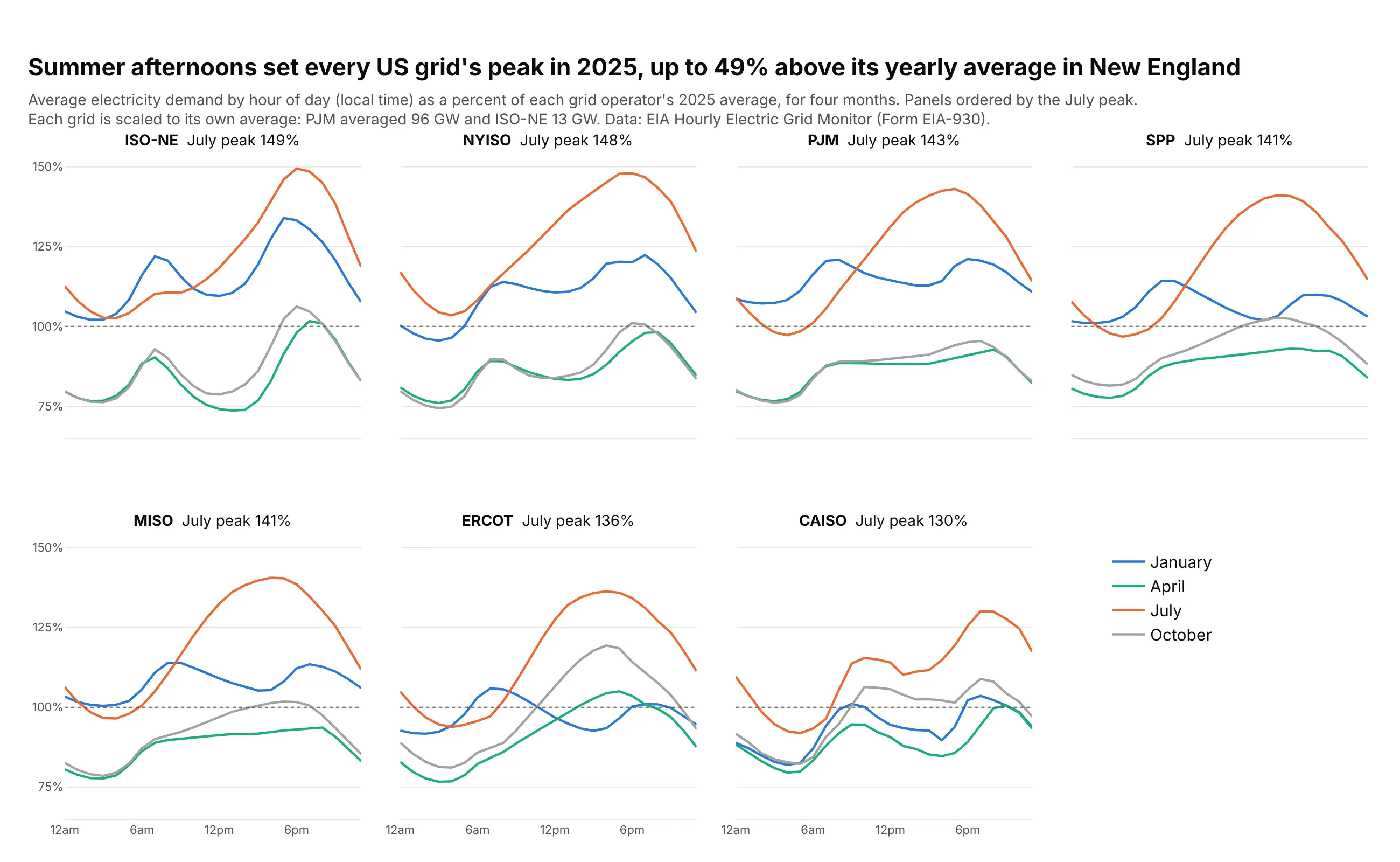
Each grid's demand is divided by its own 2025 average, so PJM (96 GW) and ISO New England (13 GW) share one axis and the panels compare shapes. In July the daily peak ran 30% to 49% above each grid's average, the most in New England. Data: EIA Hourly Electric Grid Monitor (Form EIA-930), 2025.

Tip: indexing every series to its own average lets very different sizes share one axis, so you don't need independent scales.

2. Crude oil production by state, on independent axes

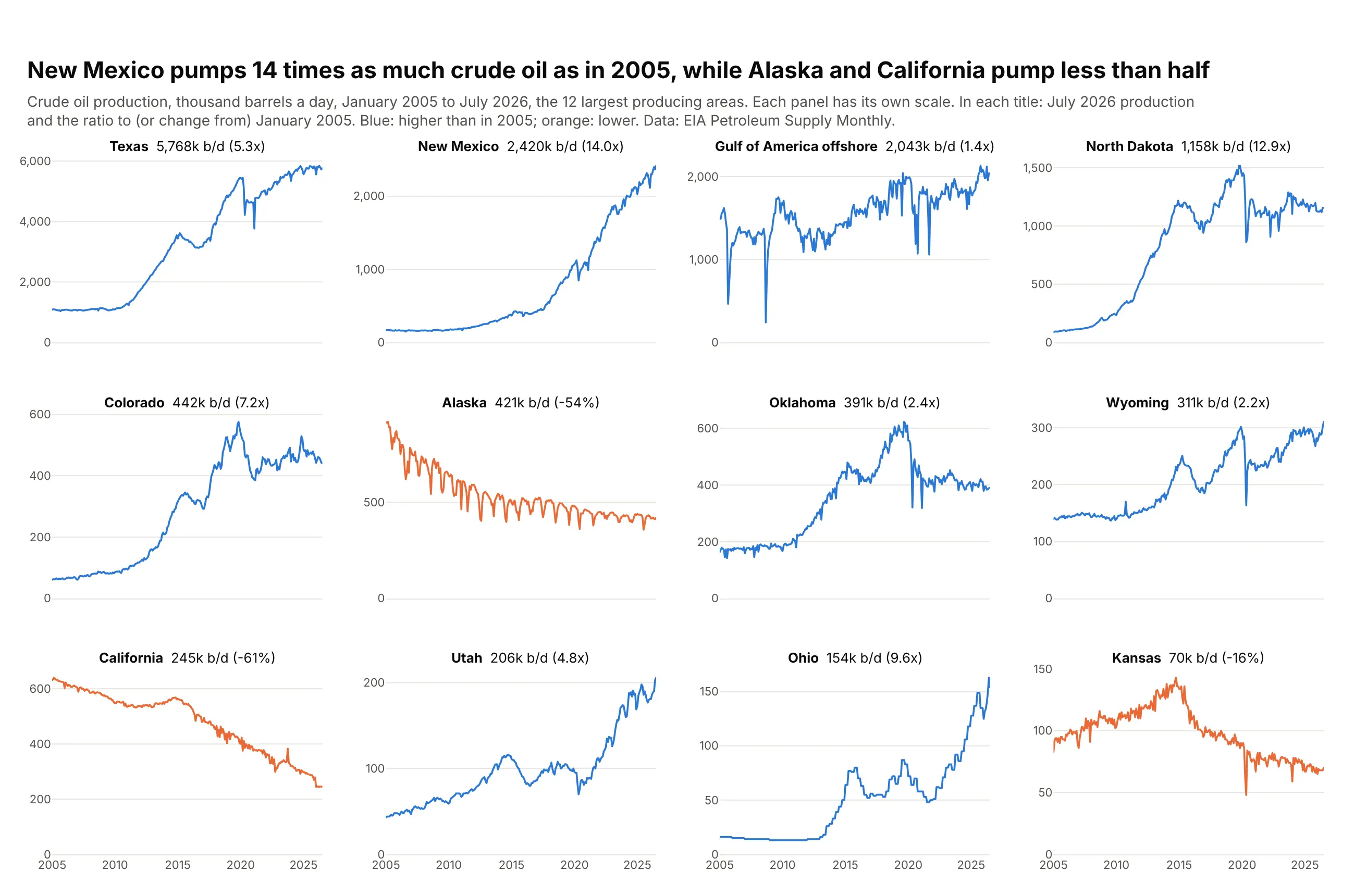
With each panel on its own scale, every state's shape is readable, and the latest value and the ratio to 2005 in each title carry the size. New Mexico now pumps 14 times as much crude as in January 2005, while Alaska and California pump less than half. Data: EIA Petroleum Supply Monthly.

Tip: fig.update_yaxes(matches=None, showticklabels=True) frees and labels every y axis, and rangemode="tozero" keeps each one honest from zero.

3. A cycle plot of US natural gas use

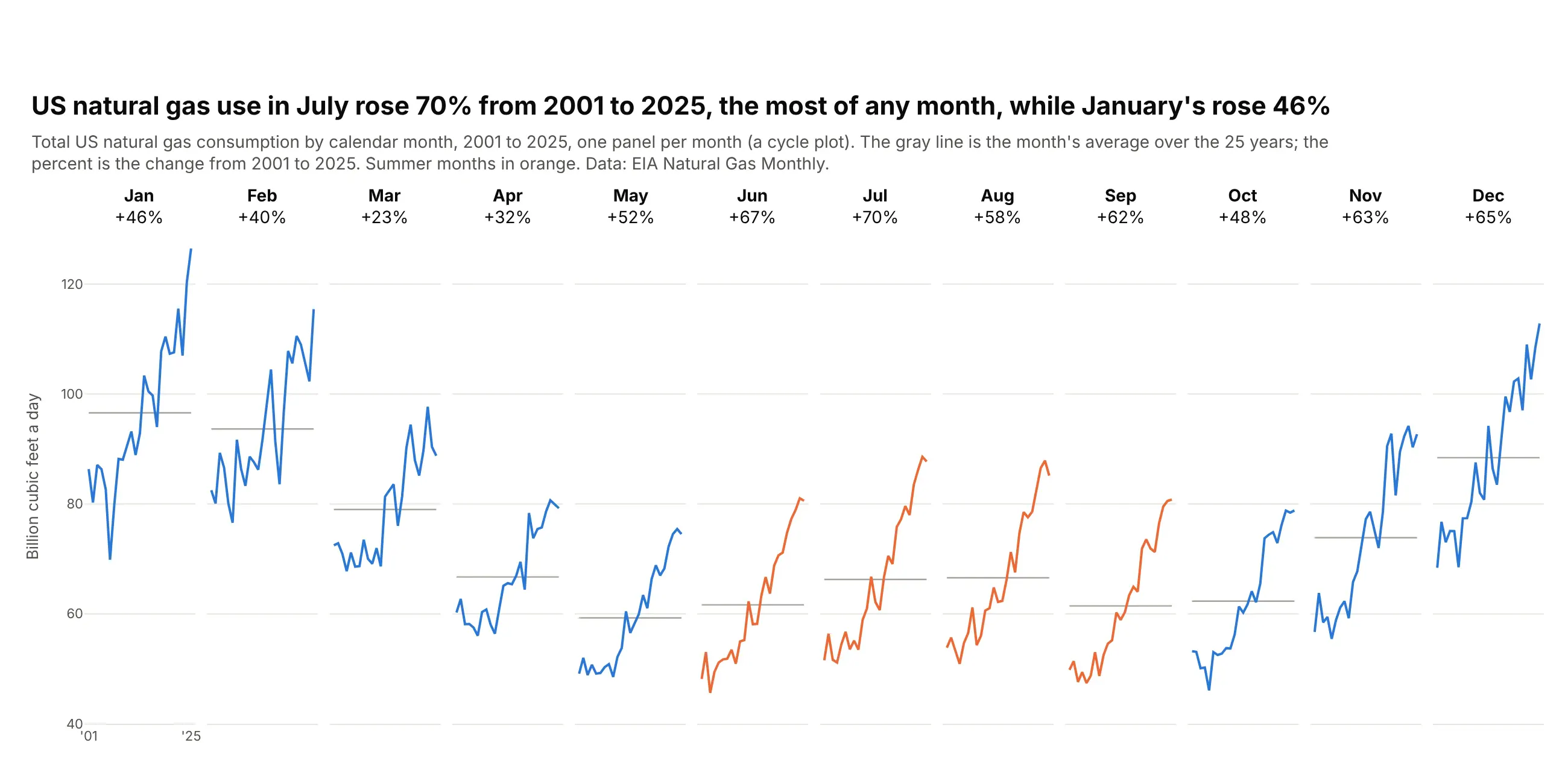
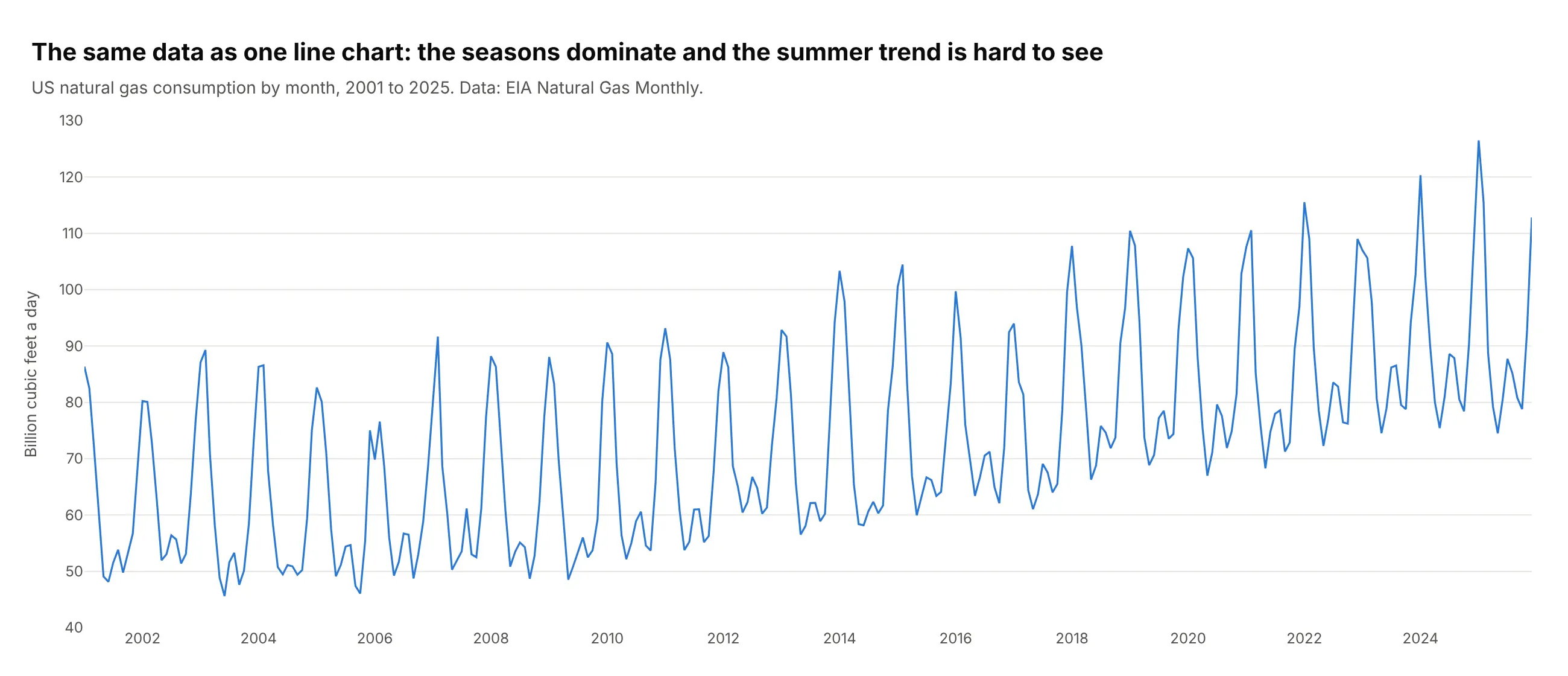
A cycle plot gives each calendar month its own panel with the years from left to right, so the seasons and the trend show up at once. July consumption rose 70% from 2001 to 2025, the most of any month, while January rose 46% and March 23%. Data: EIA Natural Gas Monthly.

Tip: make_subplots(rows=1, cols=12, shared_yaxes=True) with year labels only under the first panel keeps twelve narrow panels readable.

Another way to see it: the same data as one line chart shows the seasons as a zigzag, and the faster growth of summer consumption is hard to see.

4. Every Treasury yield curve since 2019

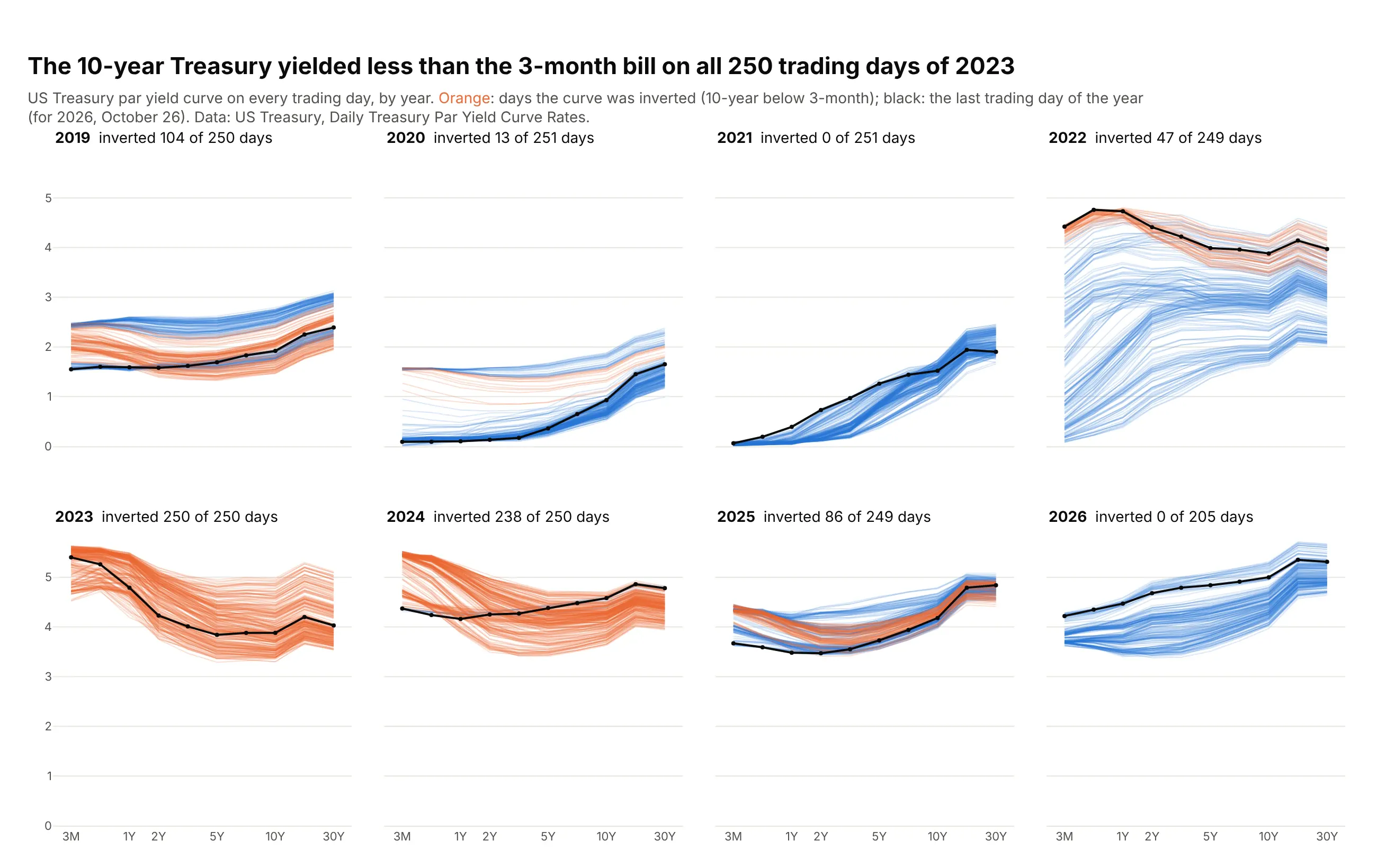
Each panel draws every trading day's yield curve in a year, orange when the 10-year yield was below the 3-month yield. The curve was inverted on all 250 trading days of 2023 and 238 of 250 in 2024, and on none so far in 2026. Data: US Treasury, Daily Treasury Par Yield Curve Rates.

Tip: all the days of one color go into one trace with None between curves, so 1,955 curves need 24 traces instead of 1,955.

5. Clinical trial starts by phase and sponsor

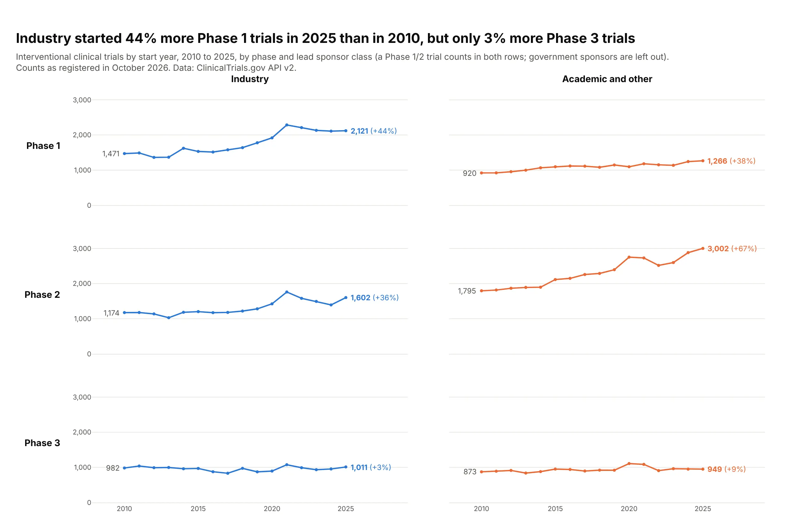
Phases run down the rows and sponsor classes across the columns, so you can compare along either. Industry started 44% more Phase 1 trials in 2025 than in 2010, but only 3% more Phase 3 trials. Data: ClinicalTrials.gov API v2.

Tip: facet_row and facet_col together make a two-way grid, and moving the row labels to the left side makes it read like a table.

6. Flu hospitalizations in every state, ranked

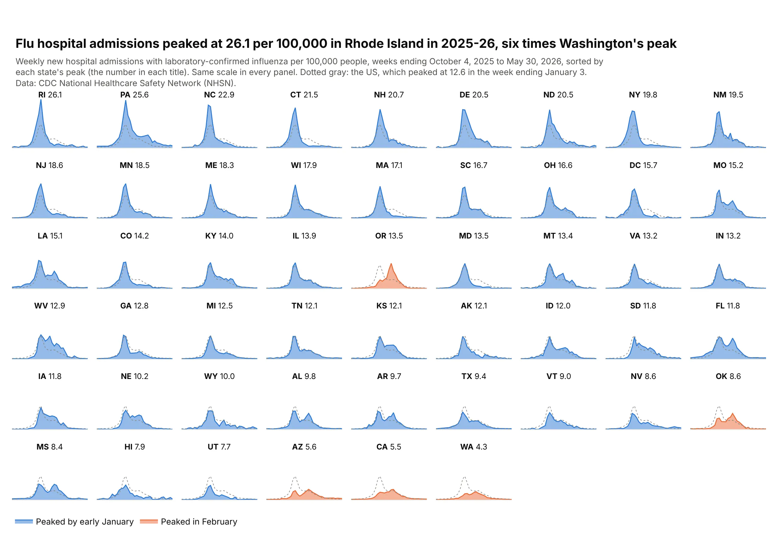
Sorting 51 sparklines by their peak turns the grid into a ranking. Rhode Island peaked at 26.1 admissions per 100,000, six times Washington's 4.3, and the five orange states peaked in February, weeks after the national peak in the week ending January 3. Data: CDC National Healthcare Safety Network (NHSN), 2025-26 season.

Tip: the national series as a dotted gray line in every panel gives each state a reference without a second axis.

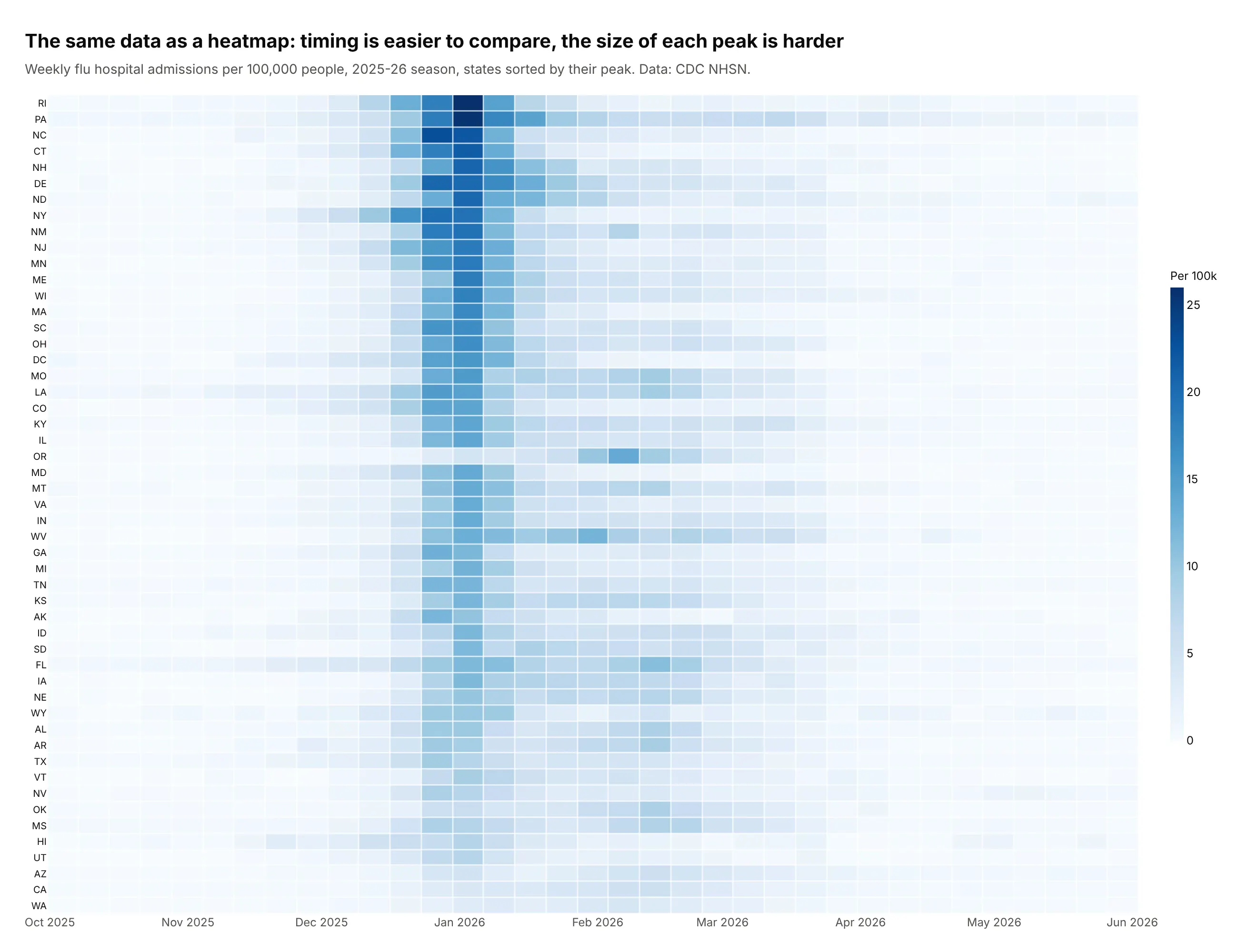
Another way to see it: a heatmap with the states in the same order shows the timing of each peak more clearly, but the size of each peak is harder to judge from color.

7. Daily highs in eight cities against their normal range

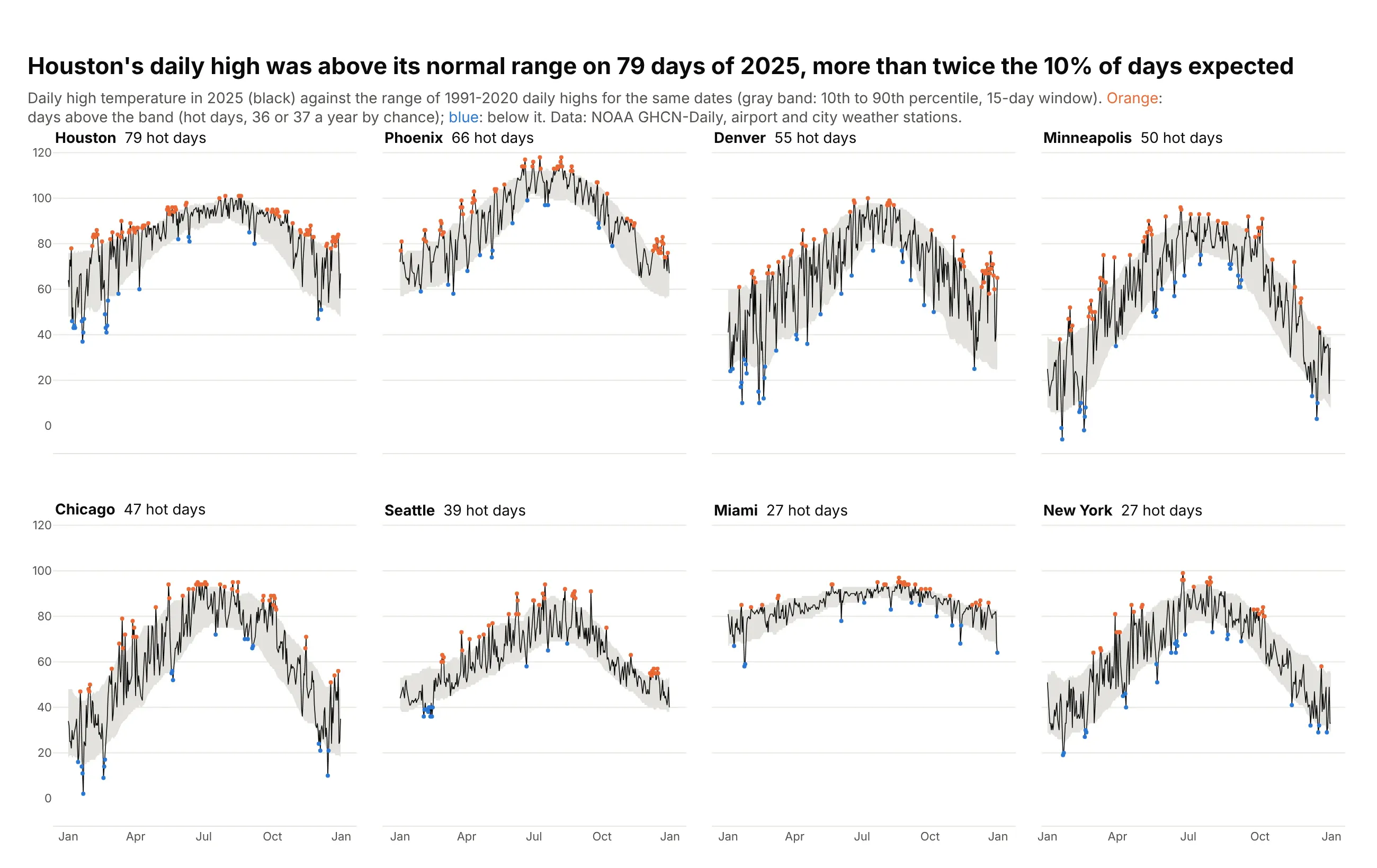
Each city gets its own band of normal daily highs, the 10th to 90th percentile for 1991-2020, so a hot day means hot for that city. By chance about 10% of days fall above the band, but Houston had 79 such days in 2025, more than twice that. Data: NOAA GHCN-Daily.

Tip: two invisible lines with fill="tonexty" draw the band, and the 2025 line goes on top so it stays visible.

8. CO2 and income by continent

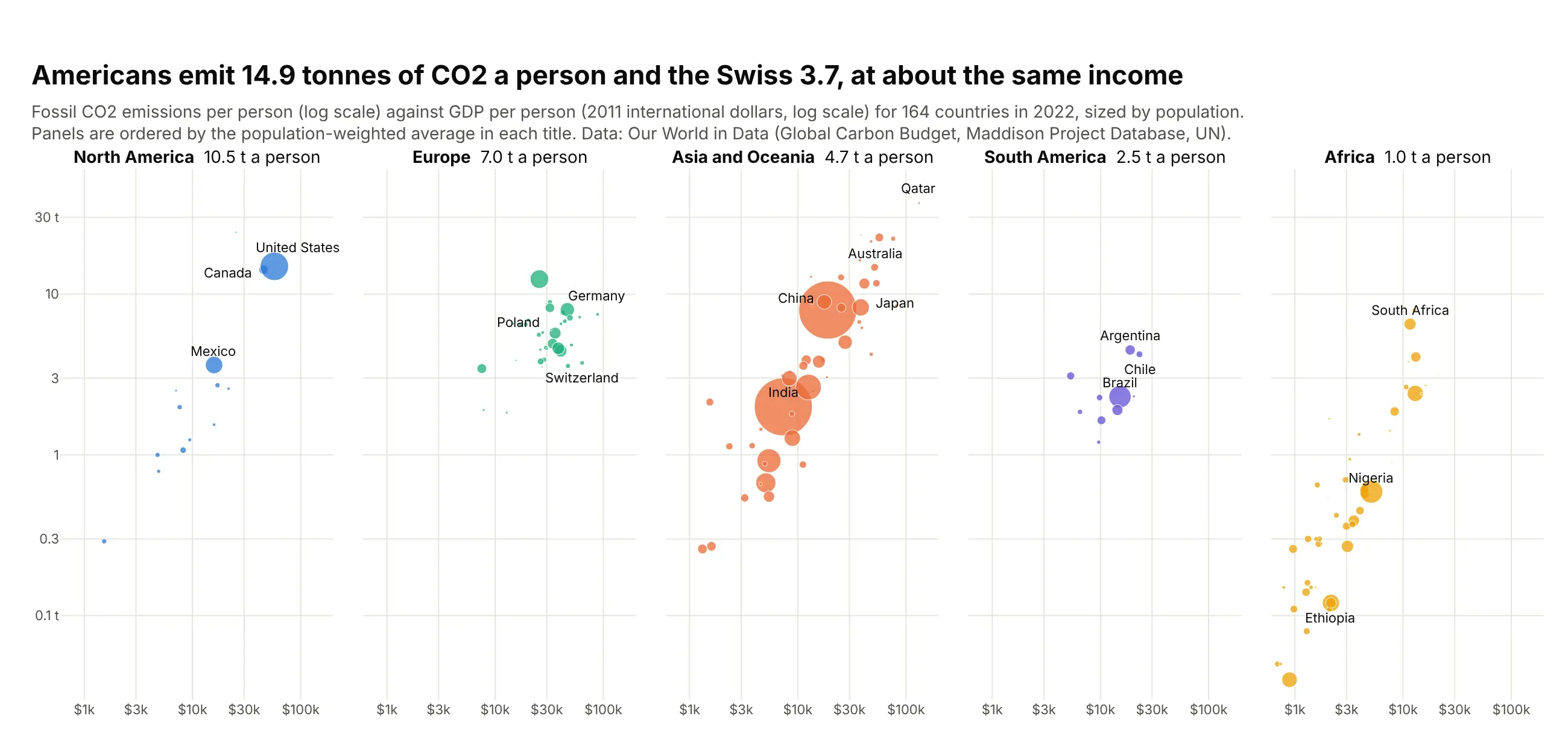
One scatter panel per continent with the same log axes shows each region's spread without five colors piled on top of each other. Americans emit 14.9 tonnes of CO2 a person and the Swiss 3.7, at about the same income. Data: Our World in Data (Global Carbon Budget, Maddison Project Database, UN), 2022.

Tip: log_x=True, log_y=True in px.scatter applies to every facet, and labels added with xref="x3" need log10 positions on a log axis.

9. Unemployment maps for four months

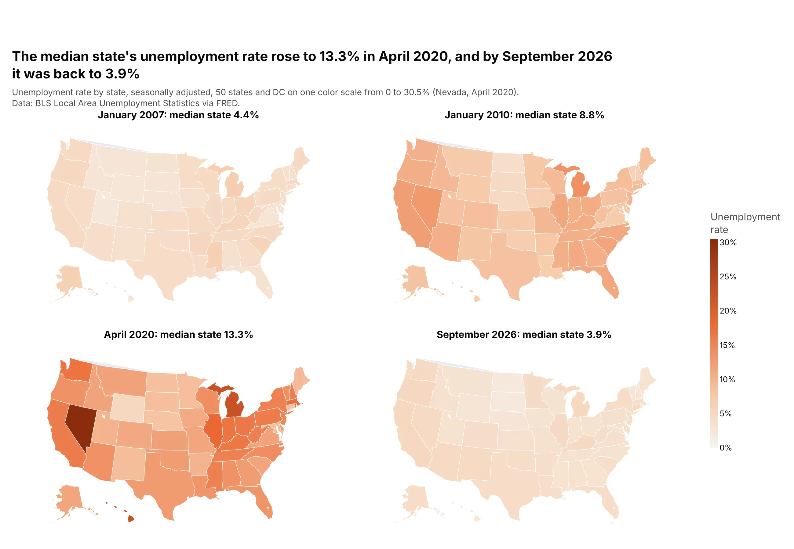
A series of maps on one color scale is the classic small multiple, used in the Statistical Atlas of the United States for the 1870 census. Four maps of the state unemployment rate show the spread after the Great Recession and the spike of April 2020, when the median state's rate reached 13.3%. Data: BLS Local Area Unemployment Statistics via FRED.

Tip: px.choropleth takes facet_col and facet_col_wrap like the other Plotly Express functions, and range_color keeps one color scale across every map. See our choropleth map guide for more.