Streamgraphs - A Complete Guide

TL;DR

• A streamgraph is a stacked area chart whose layers float around a center line instead of sitting on a zero baseline, so you can follow how each category rises and falls over time.
• Streamgraphs are also known as stream graphs and ThemeRivers, and are similar to stacked area charts and small multiples.
• Use one for many categories over time when the shapes and the turnover matter more than exact values: genres, topics, sources of electricity, waves of a disease.
• Use a stacked area chart when the total matters, a line chart or small multiples when exact values matter, and a 100% stacked area chart for shares.
• You can make a streamgraph with Plotly from go.Scatter traces in one stackgroup, with a computed baseline as an invisible first trace. The helper below does it in about 20 lines.

What is a streamgraph?

Streamgraphs look like this:

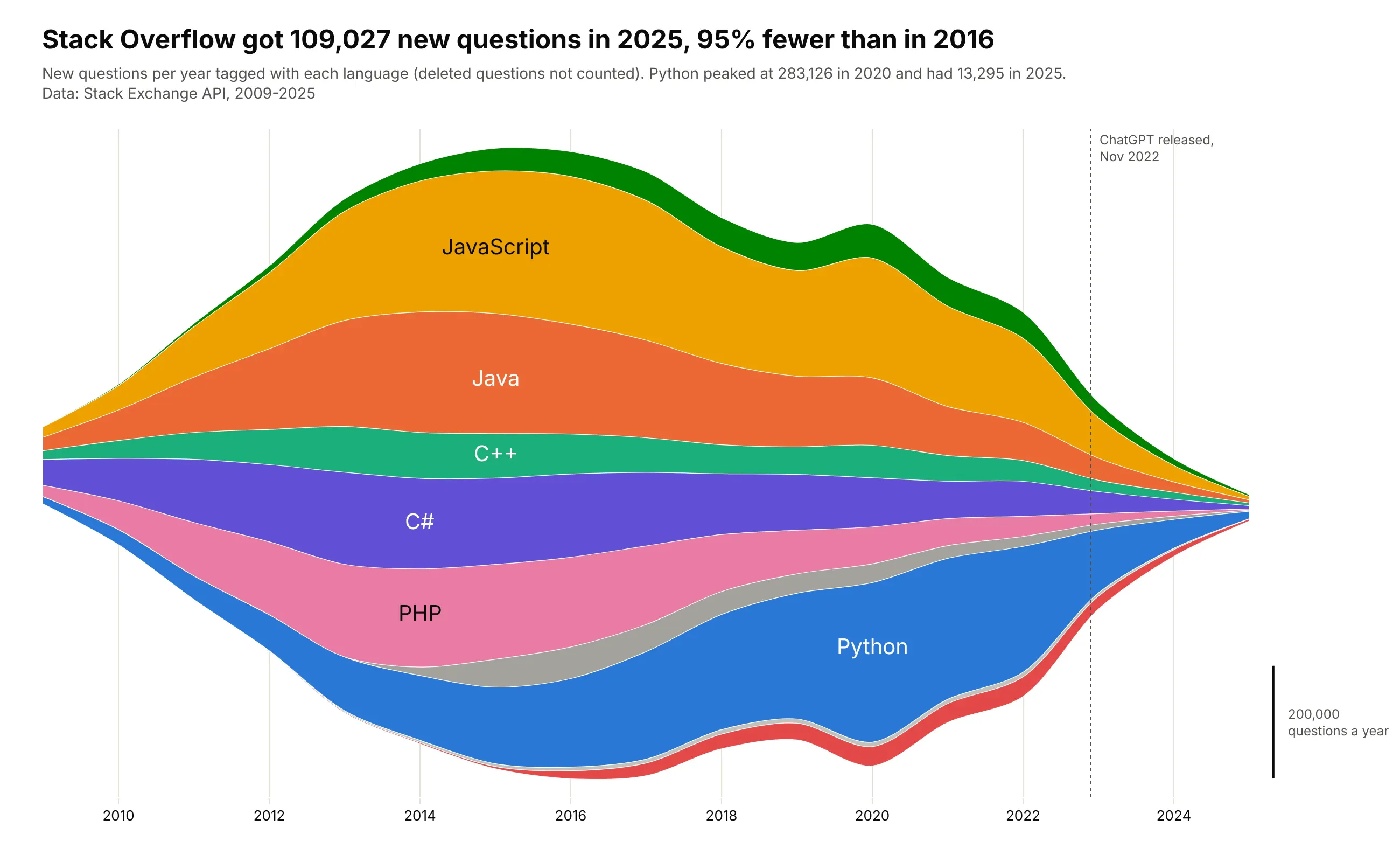
Data: Stack Exchange API, 2009-2025.

How do you read a streamgraph? In the example above, notice these things:

• Each colored layer is one language, and its thickness at any year is the number of new questions tagged with it that year. The orange JavaScript layer is the thickest one through the mid-2010s.
• The outline of the whole stream is the total, so its shape tells the story of Stack Overflow itself. It is widest around 2016 and narrows to almost nothing by 2025, when there were 95% fewer new questions.
• Follow one layer from left to right to see the mix change. The blue Python layer at the bottom keeps getting thicker while PHP and C# thin out, until it becomes the thickest layer in the stream in 2019.
• The bottom edge is a computed curve that keeps the stream centered around the middle, which is why there is no y axis. To judge how thick a layer is, hold it up against the scale bar on the right.
• A layer moves up or down when the layers under it grow or shrink, so where it sits tells you nothing about its own value. Measure each layer straight up and down instead, which shows that JavaScript peaked in 2016, the same year the whole stream was widest.

It's often used for charts like these:

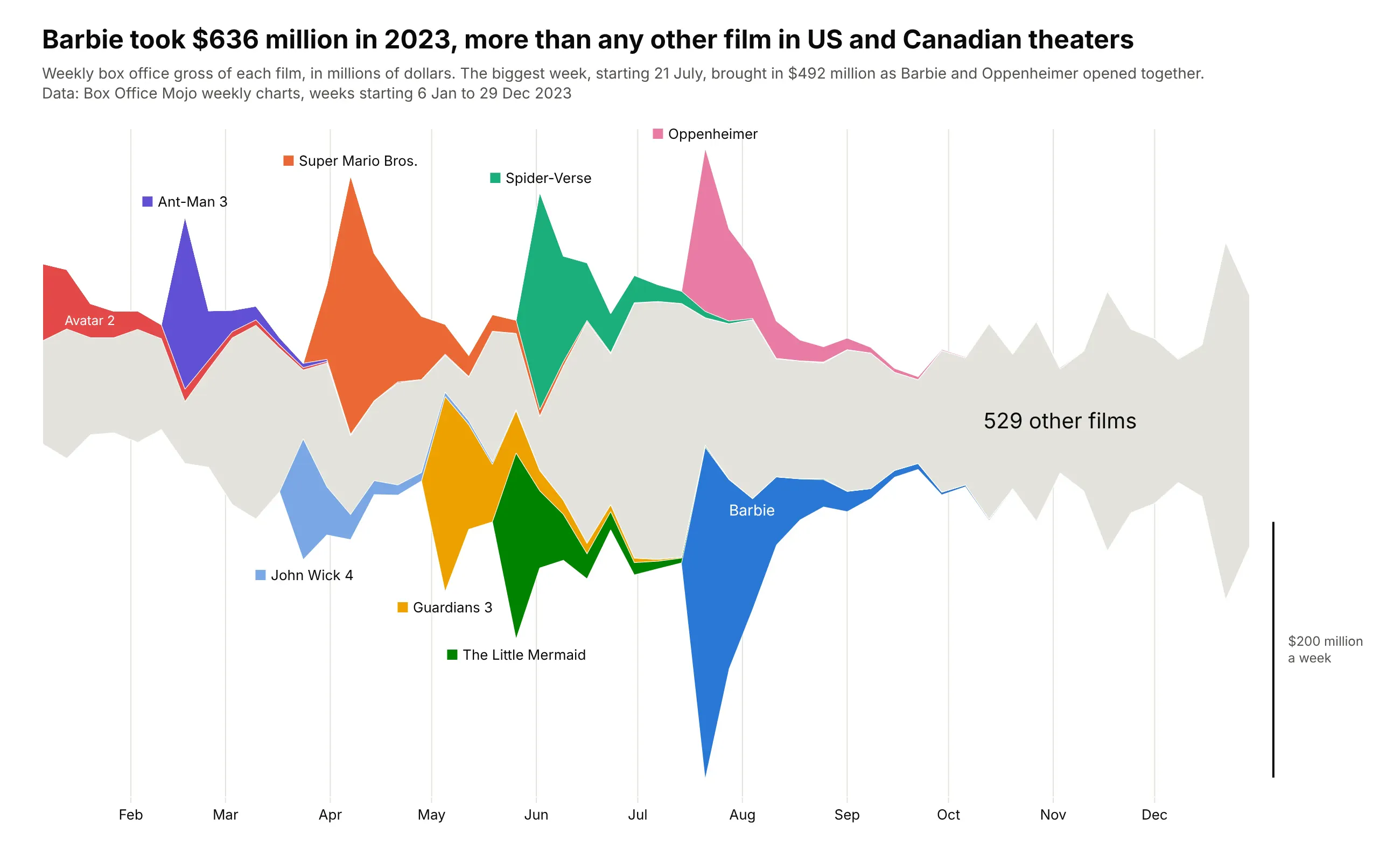
A year at the box office, the subject of The New York Times' 2008 streamgraph. Barbie took $636 million in US and Canadian theaters in 2023, and the week it opened alongside Oppenheimer brought in $492 million, the biggest week of the year. Data: Box Office Mojo weekly charts.

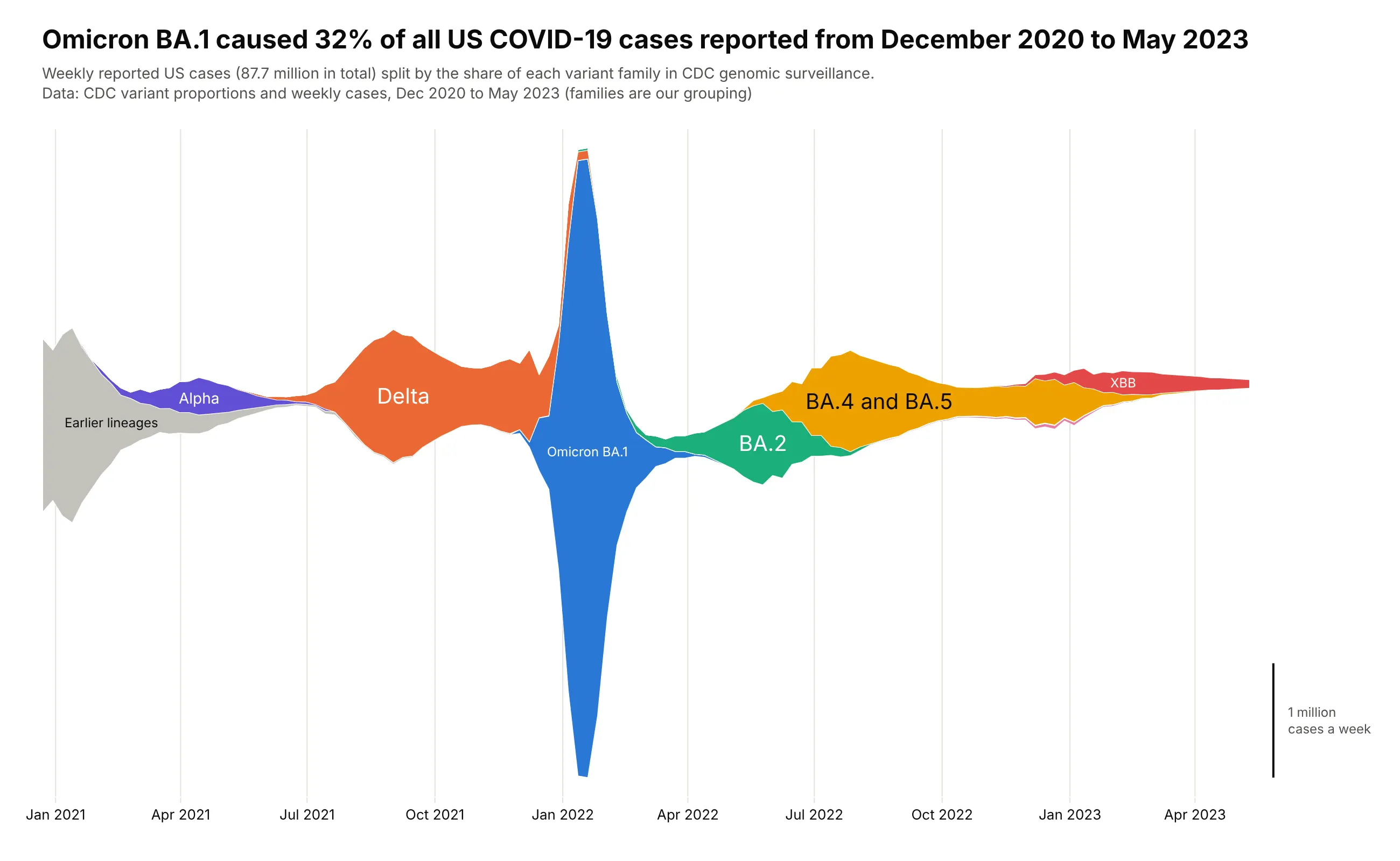
Waves that replace each other. Omicron BA.1 caused 32% of the 87.7 million US COVID-19 cases reported from December 2020 to May 2023, and 83% of its cases came in the six weeks from late December 2021 to early February 2022. Data: CDC variant proportions and weekly cases.

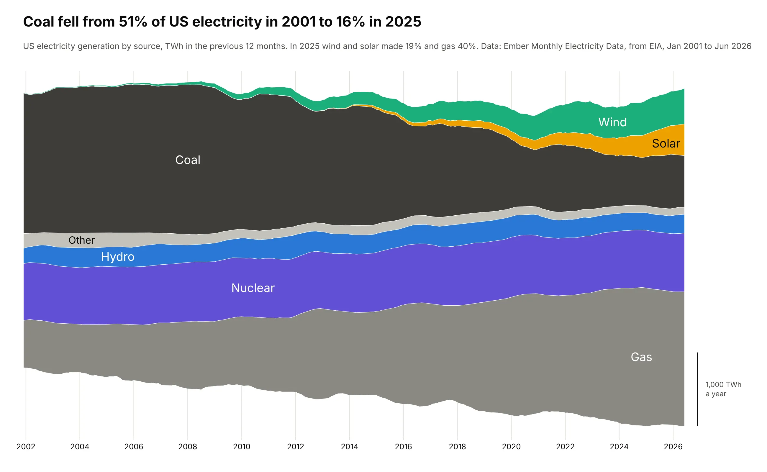
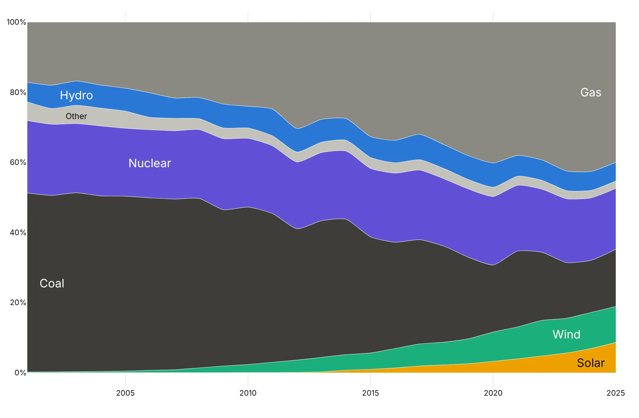
A mix that shifts over decades. Coal made 51% of US electricity in 2001 and 16% in 2025, when wind and solar together made 19%. Data: Ember Monthly Electricity Data, from EIA.

A short history

Stacked graphs of topics over time were first called ThemeRiver, by Susan Havre and colleagues at Pacific Northwest National Laboratory, who centered the layers on a line (Havre et al., 2002). Martin Wattenberg's NameVoyager (2005) stacked US baby names on a zero baseline and let visitors filter it by the letters they typed (Wattenberg, 2005). Here is that style redrawn with Plotly on the same public SSA data:

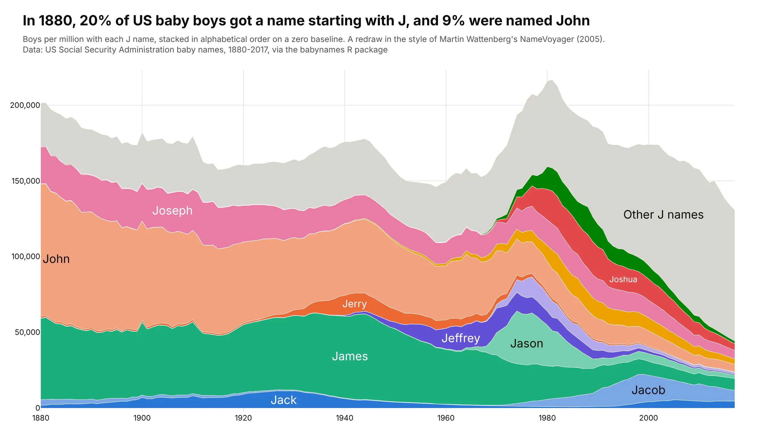
Lee Byron and Martin Wattenberg named the streamgraph in 2008 and worked out its geometry: a "wiggle" baseline that keeps the layers as flat as possible, and an inside-out layer order (Byron and Wattenberg, 2008). The same year, Byron drew The New York Times' box office graphic "The Ebb and Flow of Movies", which made the shape famous.

Alternatives to a streamgraph

Here's the same Stack Overflow data drawn six ways. Some are better for the question, some worse, some just different:

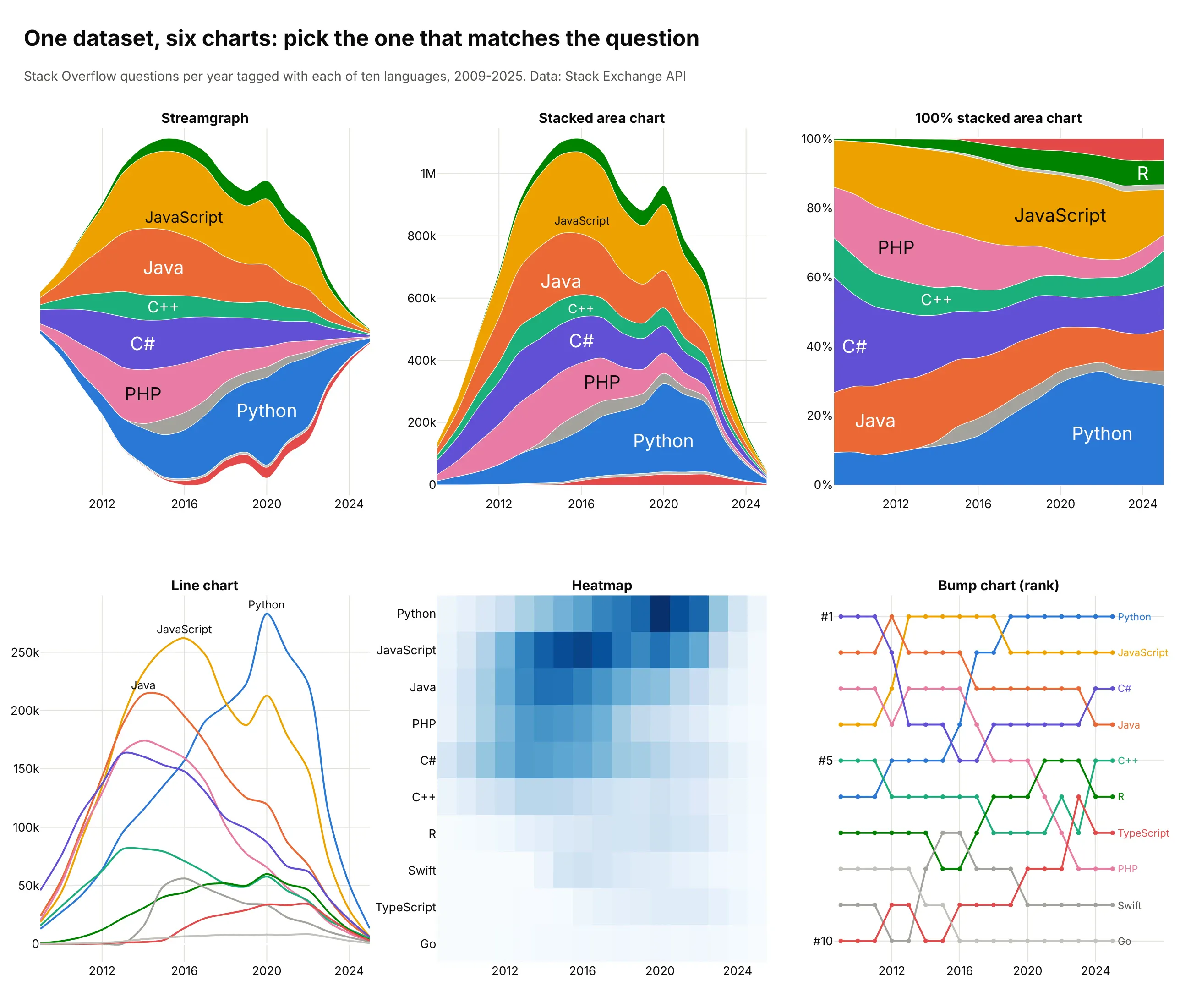
• Stacked area chart (better when the total matters). The same layers on a zero baseline, so the top edge is the total you can read against a y axis. Layers above the bottom one are still hard to compare.
• 100% stacked area chart (better for shares). Every year adds up to 100%, so you see Python's share grow while the site shrinks. It hides the collapse in volume.
• Line chart (better for exact values). Each language from zero, easy to read precisely, but ten crossing lines get crowded.
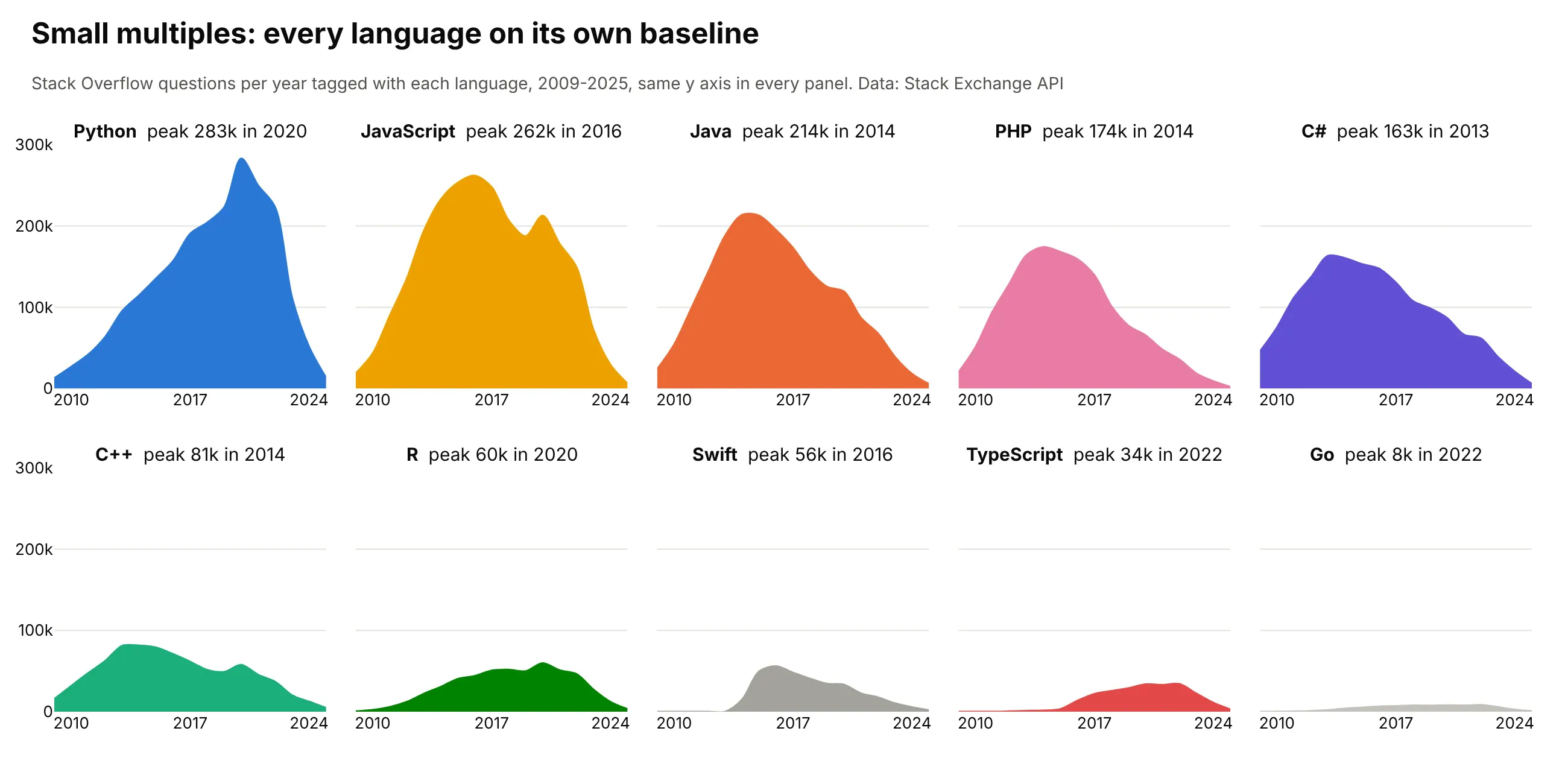
• Small multiples (better for comparing each layer's shape). One small chart per language on a shared axis, shown below.
• Heatmap (different). Rows of languages and columns of years, which scales to hundreds of categories but turns amounts into shades.
• Bump chart (different). Only the rank, which shows that Python passed JavaScript in 2019 and loses how big the gap was.

Here's where small multiples win. Each language gets its own zero baseline, so its peak and decline can be read exactly:

How to make a streamgraph

With AI

ChatGPT, Claude Code, GitHub Copilot, Cursor and other AI tools are excellent at writing Plotly code. Name Plotly in the prompt, say which baseline and layer order you want, and list the checks:

With Plotly Studio

Plotly Studio is a desktop app where you point an AI at a dataset and it builds charts and a Dash app around your questions. Ask for a streamgraph the same way:

Show a streamgraph of electricity generation by source over time, with the layers centered on a wiggle baseline and labeled inside. Add a toggle to switch between the streamgraph, a stacked area chart and a 100% stacked area chart.

Make a streamgraph in Python or JavaScript

This is the code AI tools write under the hood. The Python helper makes a streamgraph from go.Scatter traces: it computes Byron and Wattenberg's wiggle baseline and stacks the layers on top of it:

The examples in this guide use a fuller version of the same helper with the inside-out order, labels inside the layers, a scale bar and silhouette, zero and normalized baselines. In JavaScript, plotly.js builds the same thing from the same traces. This one uses the simpler silhouette baseline, minus half of each year's total:

A plain stacked area chart, the same layers on a zero baseline, needs no helper. In Python it's one line, px.area(df, x="year", y="twh", color="source"); in JavaScript it's the scatter traces above without the invisible baseline trace; and in React you pass those traces as the data prop of the Plot component from react-plotly.js.

Share it

Every Plotly chart has a Share chart button (the cloud icon in its toolbar) that uploads it to Plotly Cloud and gives you a link. Only you can see it until you change its visibility.

For a live app, put the chart in a Dash app and publish it with the Plotly Cloud CLI. Coding agents can run these commands for you:

If your data has to stay in your own cloud or data center, publish to Dash Enterprise instead.

Dos and don'ts

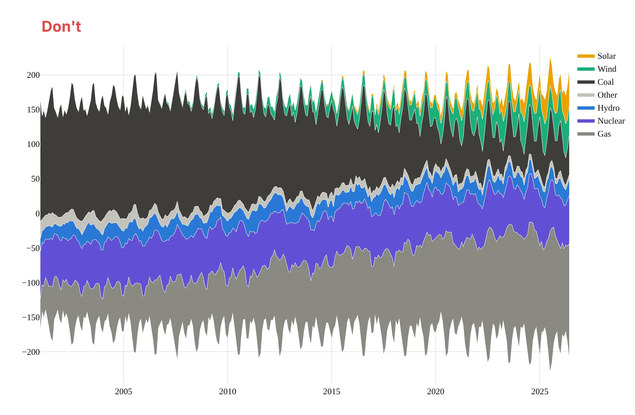
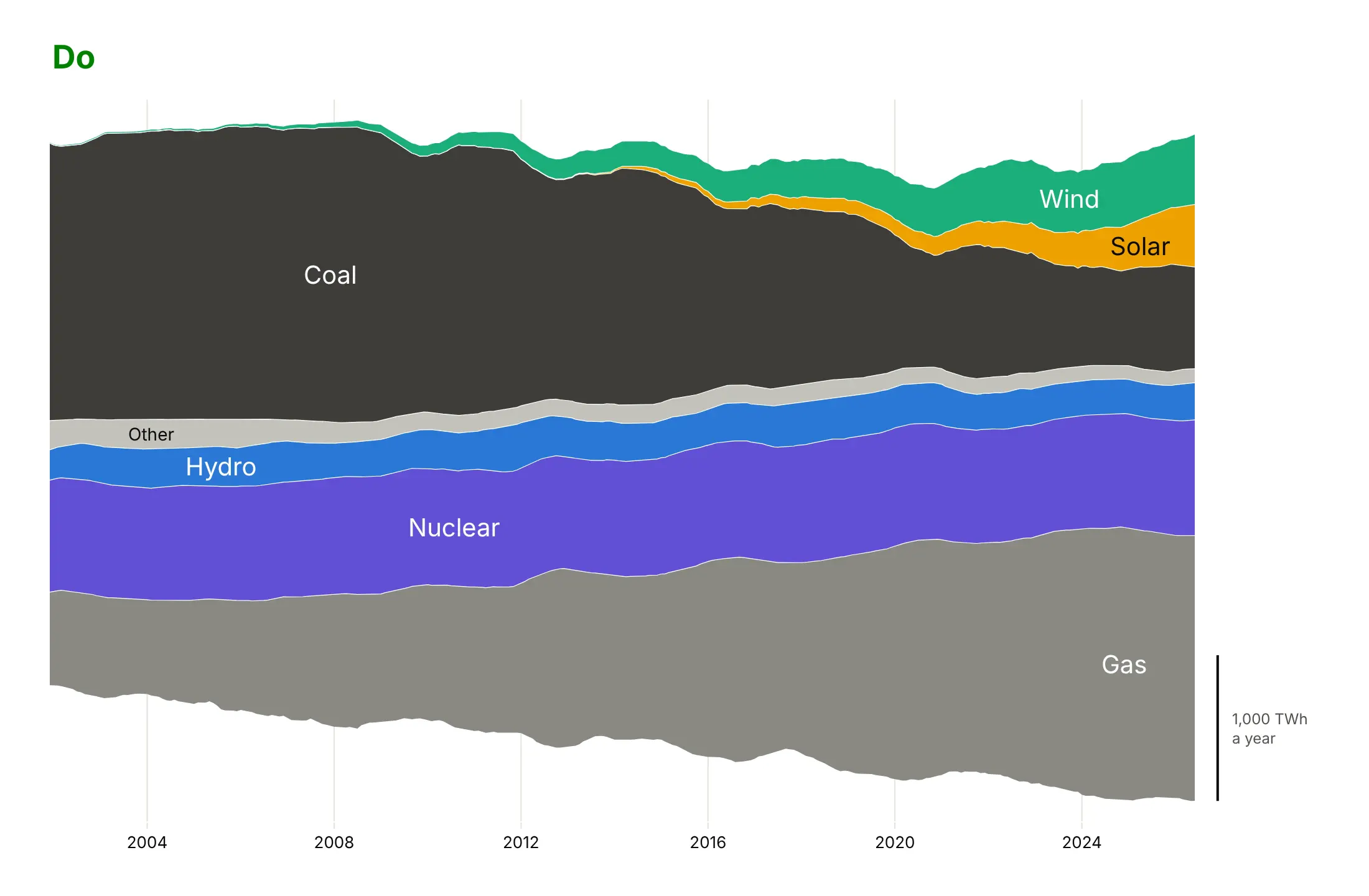
A streamgraph is easy to make noisy, because every wobble in one layer moves all the layers above it. Here is the same electricity data both ways, with the same colors and layer order.

Don't plot raw monthly values with seasonal spikes, keep a y axis whose negative numbers mean nothing, or use a hard-to-read default serif font:

Do smooth the data to the time scale of the story (here a 12-month rolling sum), label the layers inside, and replace the y axis with a scale bar:

Pick a baseline

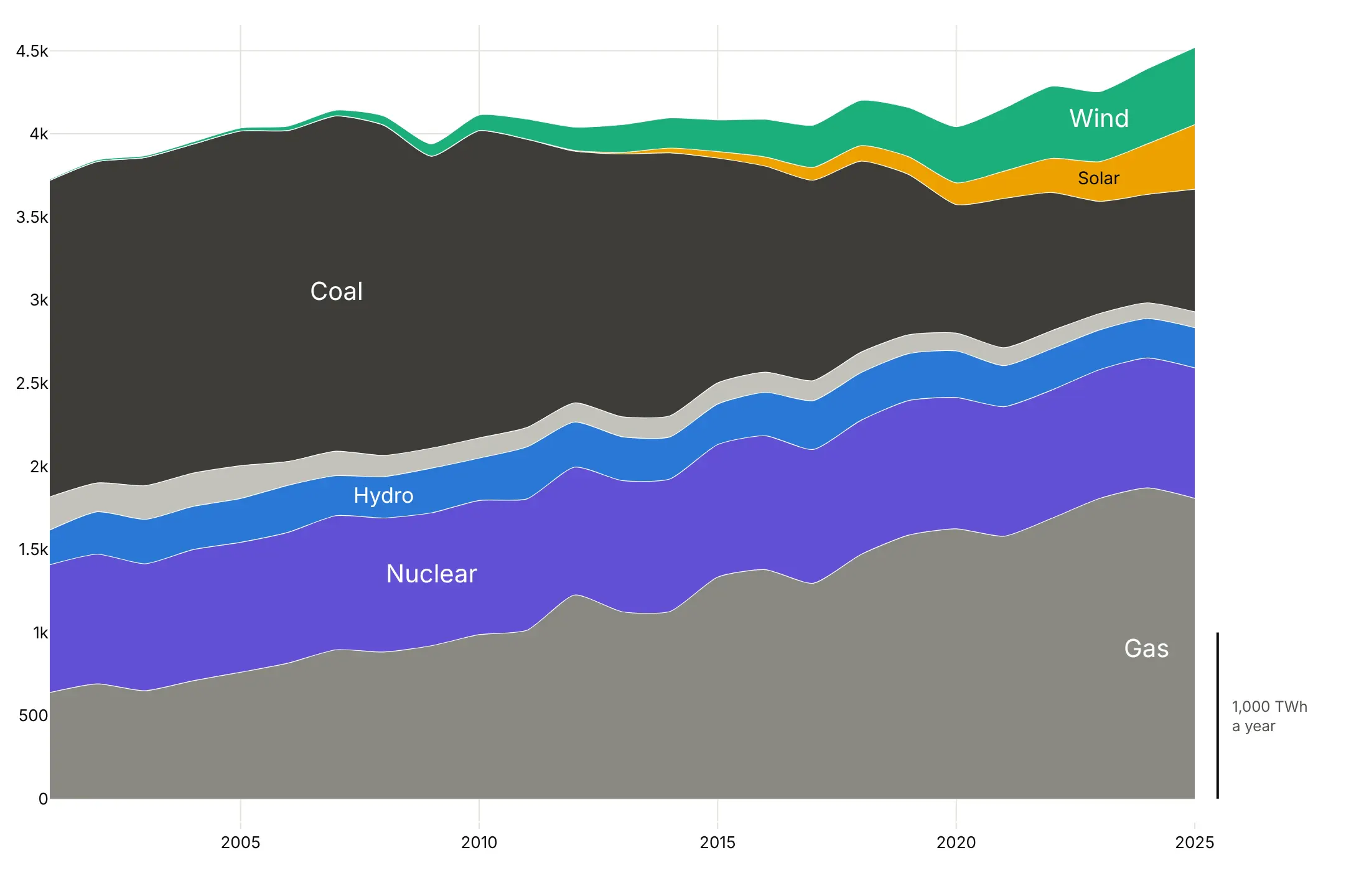
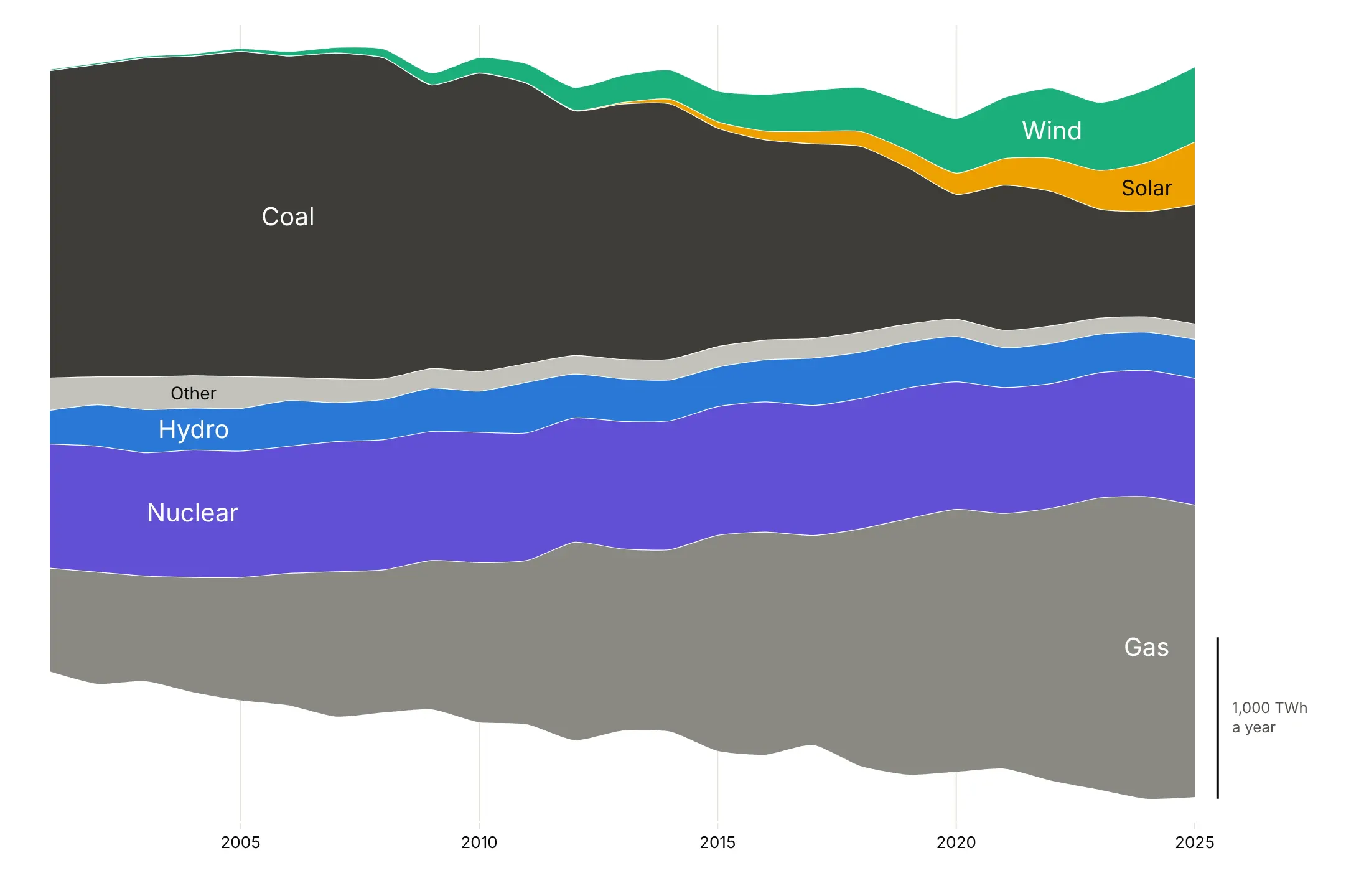
The baseline decides where the stack starts. Here are four on the same annual electricity data.

Zero. An ordinary stacked area chart, where the top edge is the total.

Silhouette. Symmetric around zero, as in ThemeRiver, so the outline shows the total as a width.

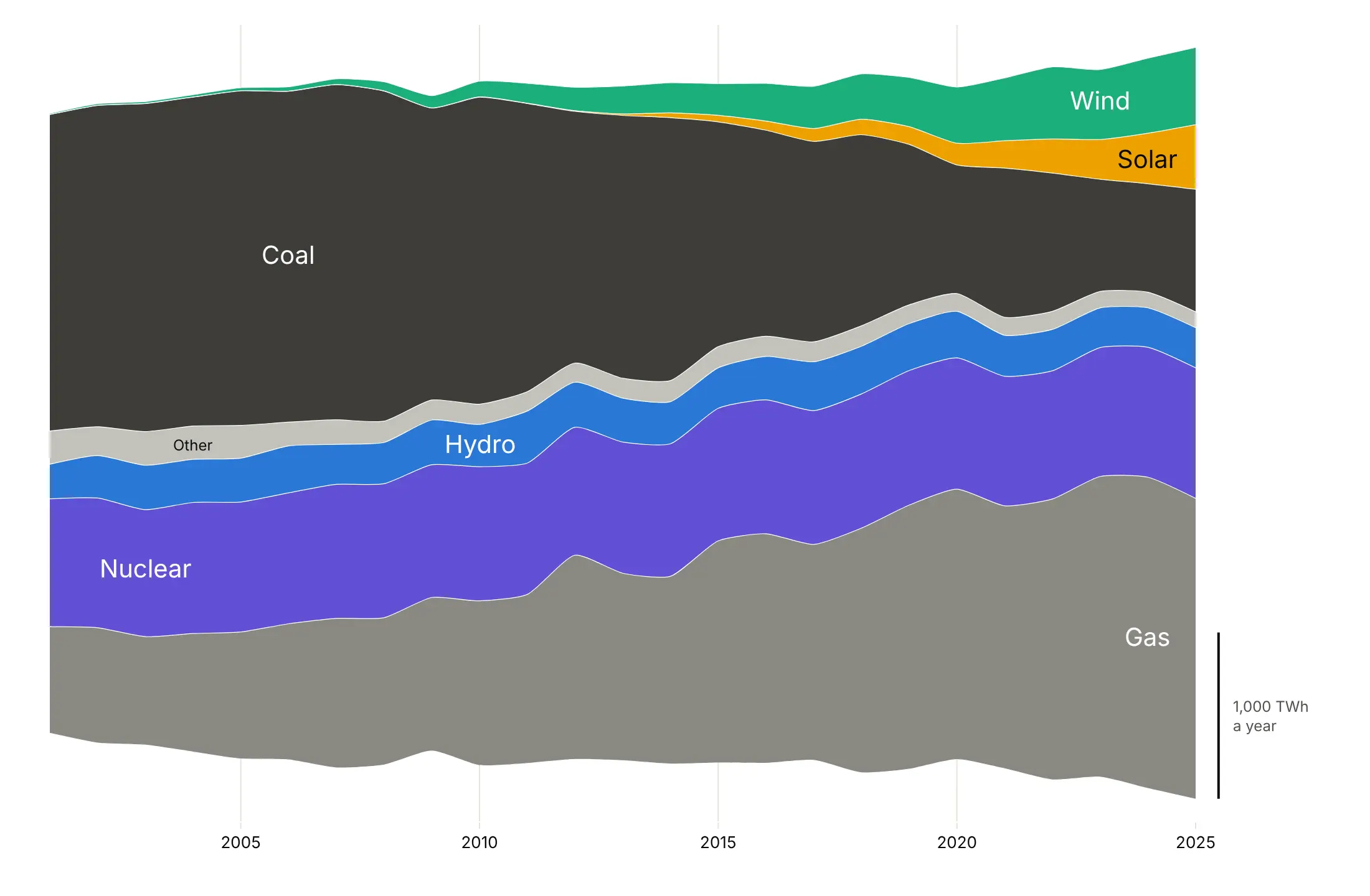
Wiggle. Byron and Wattenberg's baseline moves each year so the layers, weighted by their thickness, tilt as little as possible. It's the best default for reading individual layers.

Normalized. Every year adds up to 100%, so only the mix shows: coal falls from about half to under a fifth.

Order the layers

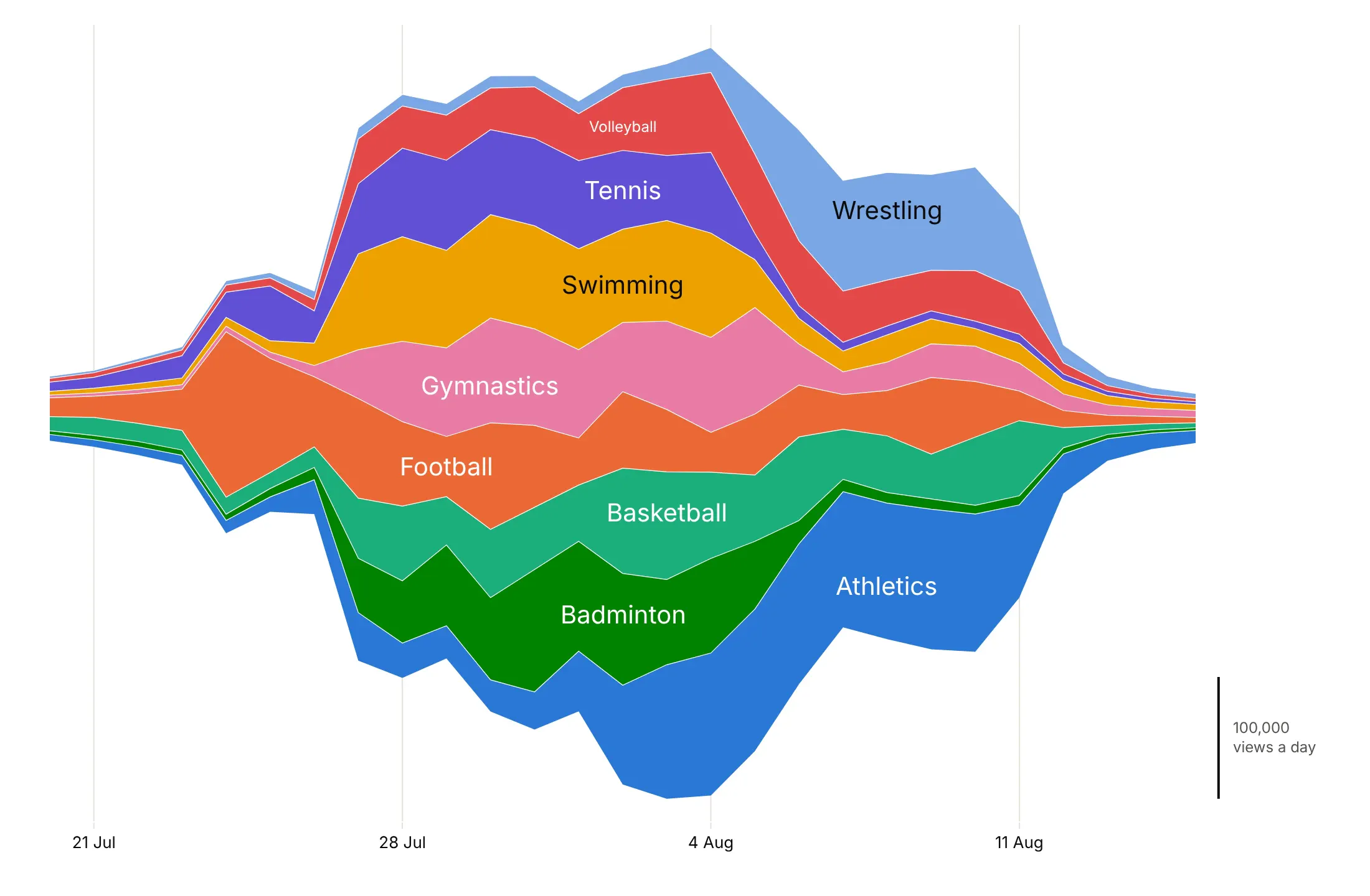
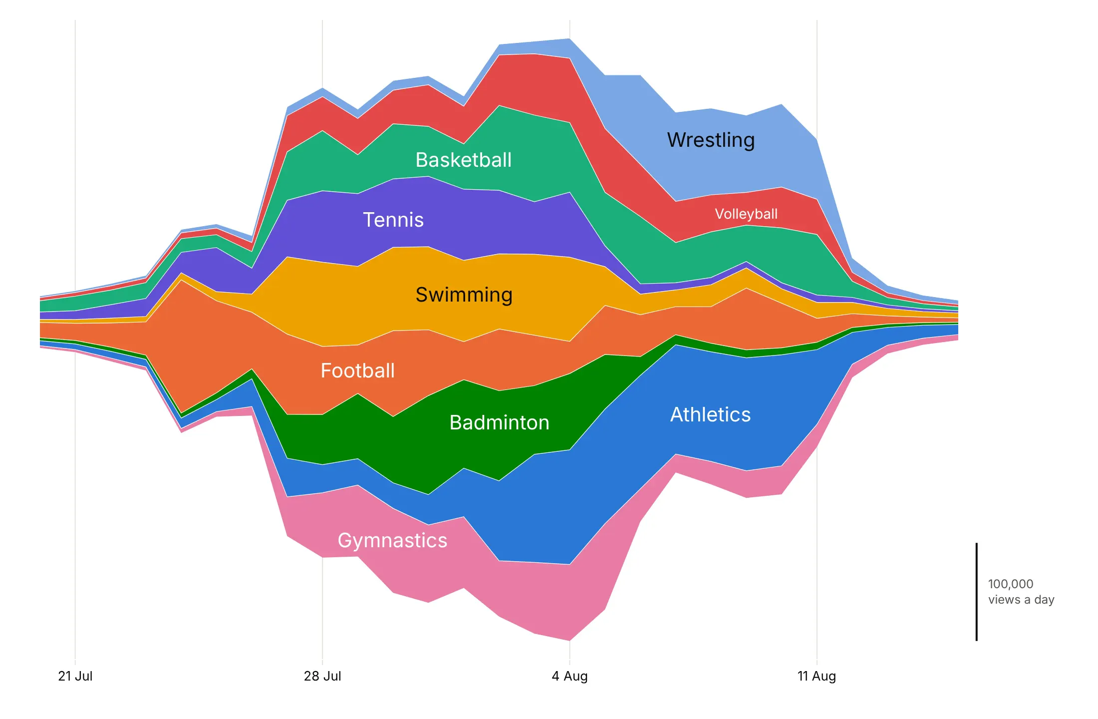
Order matters as much as the baseline. Here are the nine most-viewed Paris 2024 sport articles two ways, both on the wiggle baseline.

Alphabetical. Early and late peaks sit next to each other, and the layers move up and down by 19,024 views a day on average (our measure of Byron and Wattenberg's wiggle).

Inside-out. Layers sorted by the day they peak, earliest in the middle and later ones added alternately above and below. The wiggle drops 9%, to 17,288 views a day, and the first-week sports sit together in the middle.

Checklist

Do

• Write a title that states the takeaway, and label layers inside where they are thickest.
• Smooth or aggregate to the time scale of the story (rolling sums, weeks, years).
• Use the inside-out order, or put steady layers in the middle and spiky ones on the outside.
• Fold small categories into one gray "Other" layer.
• Replace the y axis with a scale bar, and keep exact values in the hover.

Don't

• Show a y axis with negative numbers on a centered stream.
• Use a streamgraph when readers need exact values or the total over time.
• Draw more than about 10-12 colored layers.
• Use splines on a few hundred thousand points; they draw slowly (see the FAQ).

Options to customize

These are the go.Scatter and layout options a streamgraph is built from. The full list is in the Plotly filled area documentation and the scatter reference.

1. stackgroup: traces with the same value are stacked on each other, in the order they are added.
2. The baseline trace: an invisible first trace in the stackgroup (fill="none", line.width=0, hoverinfo="skip") whose y is the computed baseline.
3. fill="tonexty": fills each layer down to the one below it.
4. groupnorm="percent": set on the first trace of a stackgroup to make a 100% stacked area chart without computing shares yourself.
5. line.shape="spline", line.smoothing: smooth curves through the points; 0.6-1.0 suits yearly data.
6. line.width, line.color: a thin white line between layers.
7. fillcolor: one fixed color per layer, the same in every chart of the series.
8. hovertemplate: the exact value of each layer, for example "Coal: %{y:,.0f} TWh<extra></extra>".
9. hovermode="x unified" (layout): one hover box with every layer's value at that date.
10. stackgaps: what to do with missing values, infer zero (default) or interpolate.
11. yaxis.visible=False (layout): hide an axis whose numbers mean nothing once the baseline moves.
12. add_annotation: layer labels inside the stream and a scale bar with add_shape.
13. xaxis.dtick, tickformat: years or dates on the time axis.

More streamgraph examples

Ten more streamgraphs built from real public data, each with its source, the technique that makes it work and a prompt to rebuild it.

1. Where US crude oil imports come from

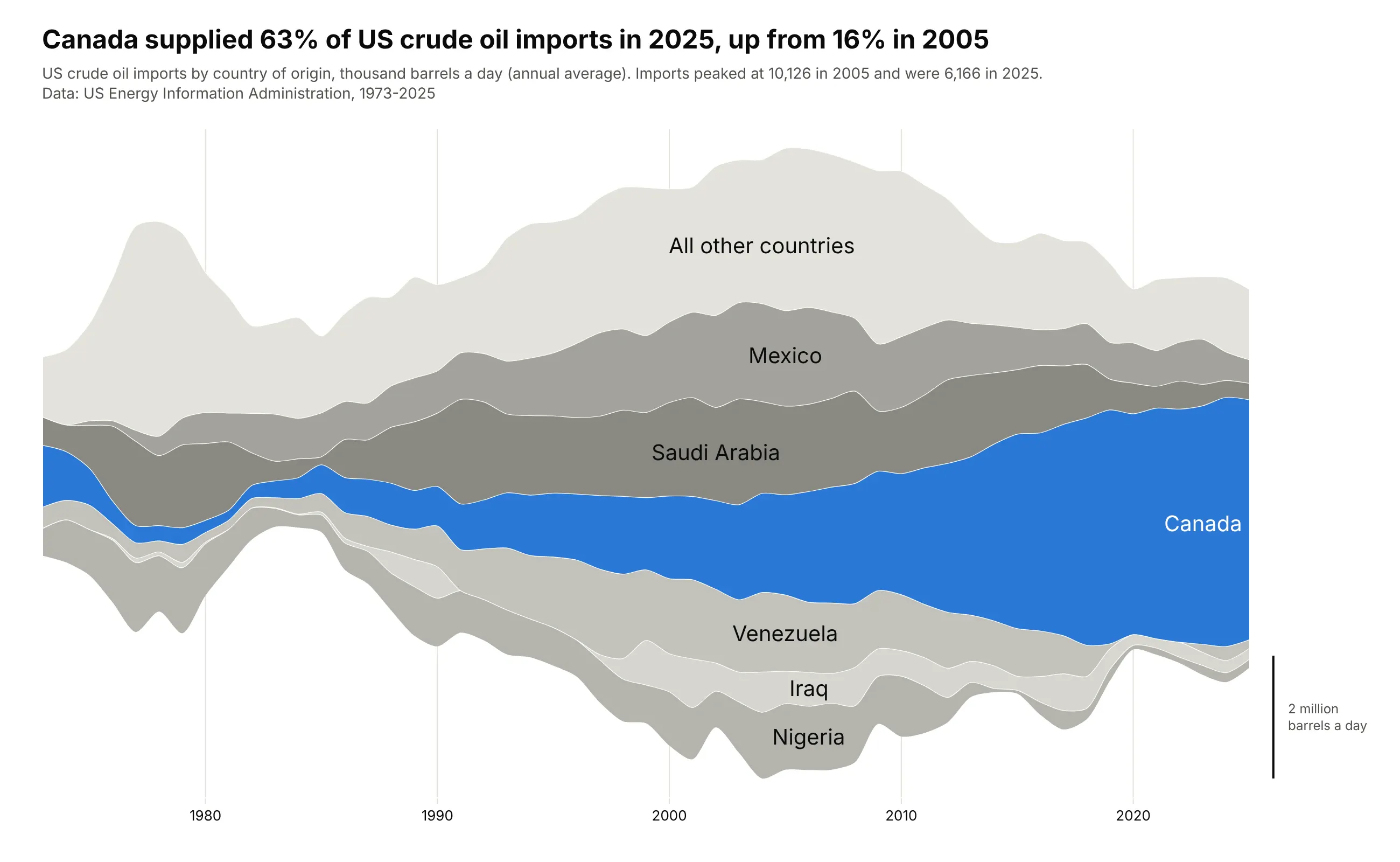
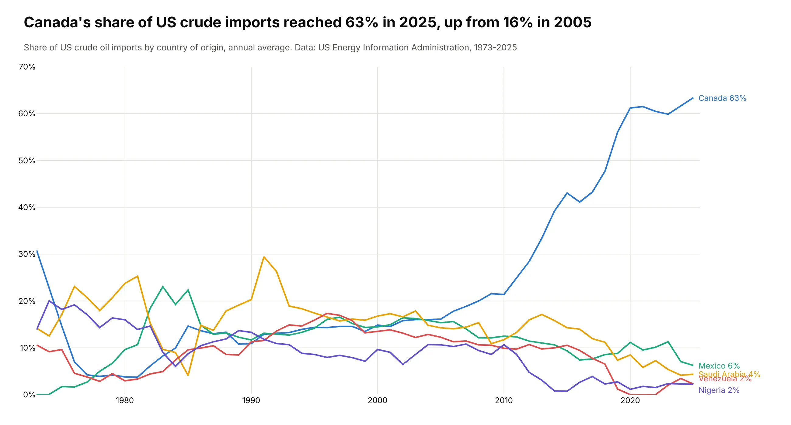
Canada supplied 63% of US crude oil imports in 2025, up from 16% in 2005, while Saudi Arabia, Venezuela, Mexico and Nigeria faded. Total imports peaked at 10,126 thousand barrels a day in 2005 and were 6,166 in 2025. Data: US Energy Information Administration, imports by country of origin, 1973-2025.

Tip: one highlighted layer on gray neighbors makes the main story read first, and the grays still show who Canada replaced.

Another way to see it: a line chart of each supplier's share shows the climb exactly (Canada passed 60% in 2020), but loses the fall in total imports since 2005.

2. Who emits the world's CO2

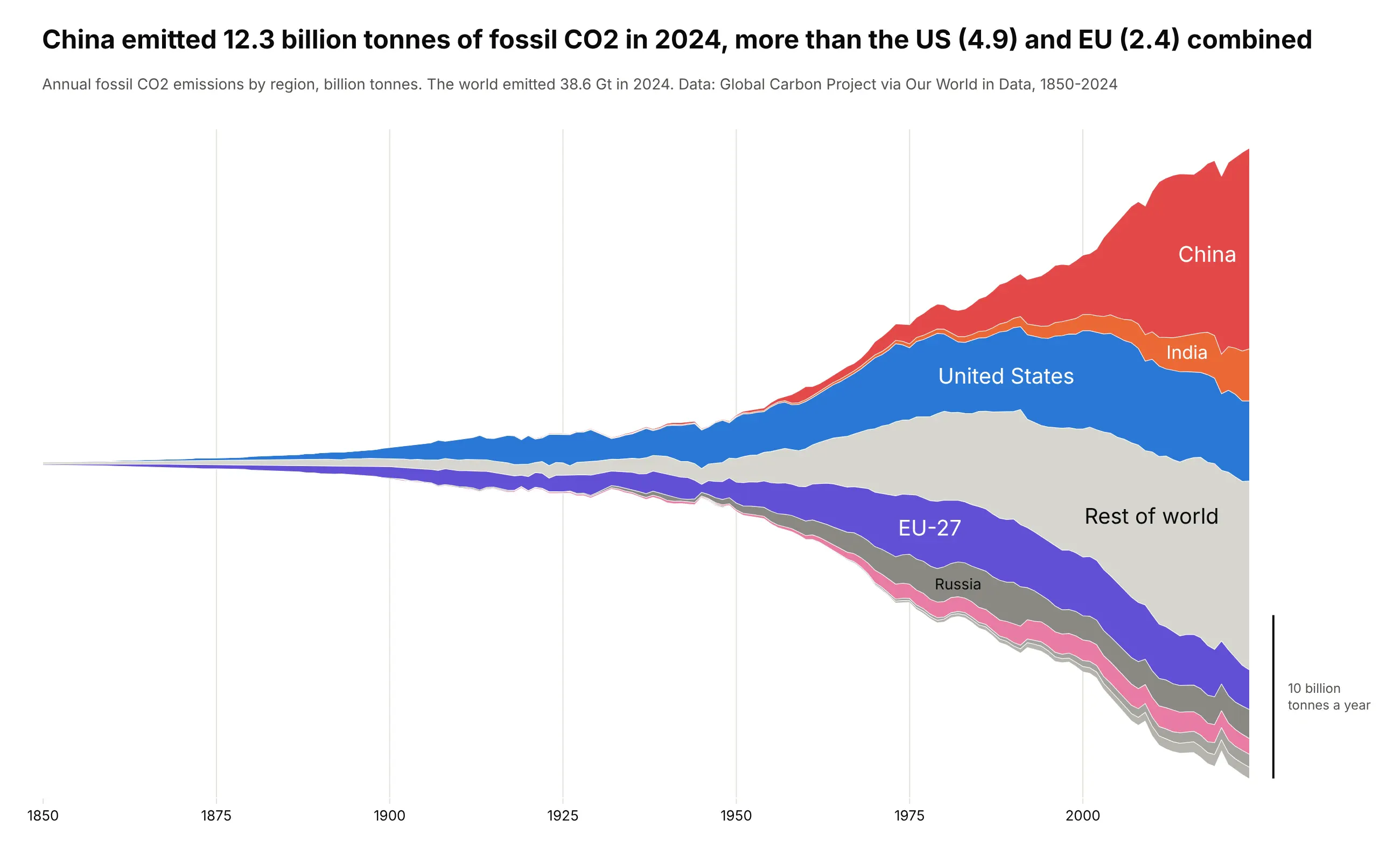
China emitted 12.3 billion tonnes of fossil CO2 in 2024, more than the US (4.9) and the EU (2.4) combined, out of 38.6 billion for the world. The stream starts as a thread in 1850 and shows who drove each era of growth. Data: Global Carbon Project via Our World in Data.

Tip: the silhouette baseline keeps the stream symmetric, so its width reads as the world total, which matters here as much as the layers.

3. Foreign holders of US Treasuries

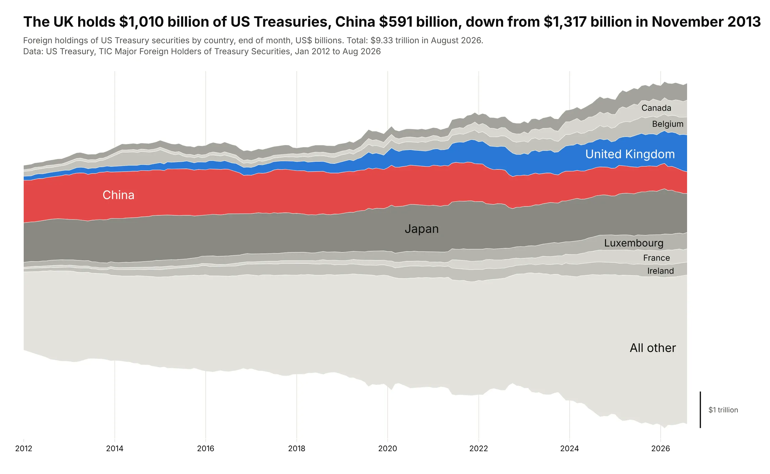
China held $1,317 billion of US Treasuries in November 2013 and $591 billion in August 2026, while the United Kingdom grew to $1,010 billion. Foreign holdings rose to $9.33 trillion in total. Data: US Treasury, TIC Major Foreign Holders of Treasury Securities, January 2012 to August 2026.

Tip: placing the two layers you want to compare next to each other in the middle, instead of using the inside-out order, makes their thickness easy to compare.

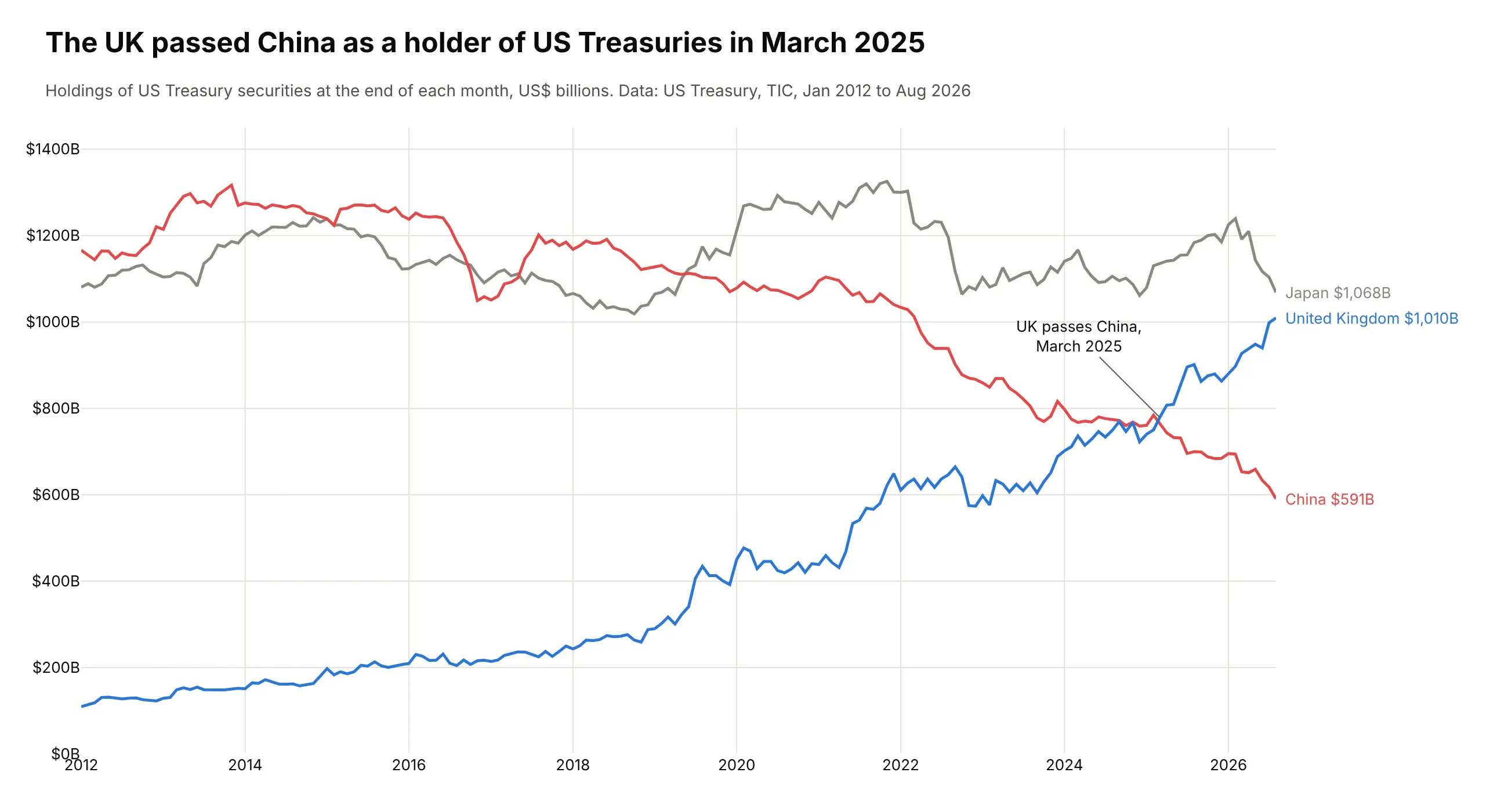
Another way to see it: a line chart of China, Japan and the UK shows the exact month the UK passed China, March 2025.

4. When the total is the story: the Fed's balance sheet

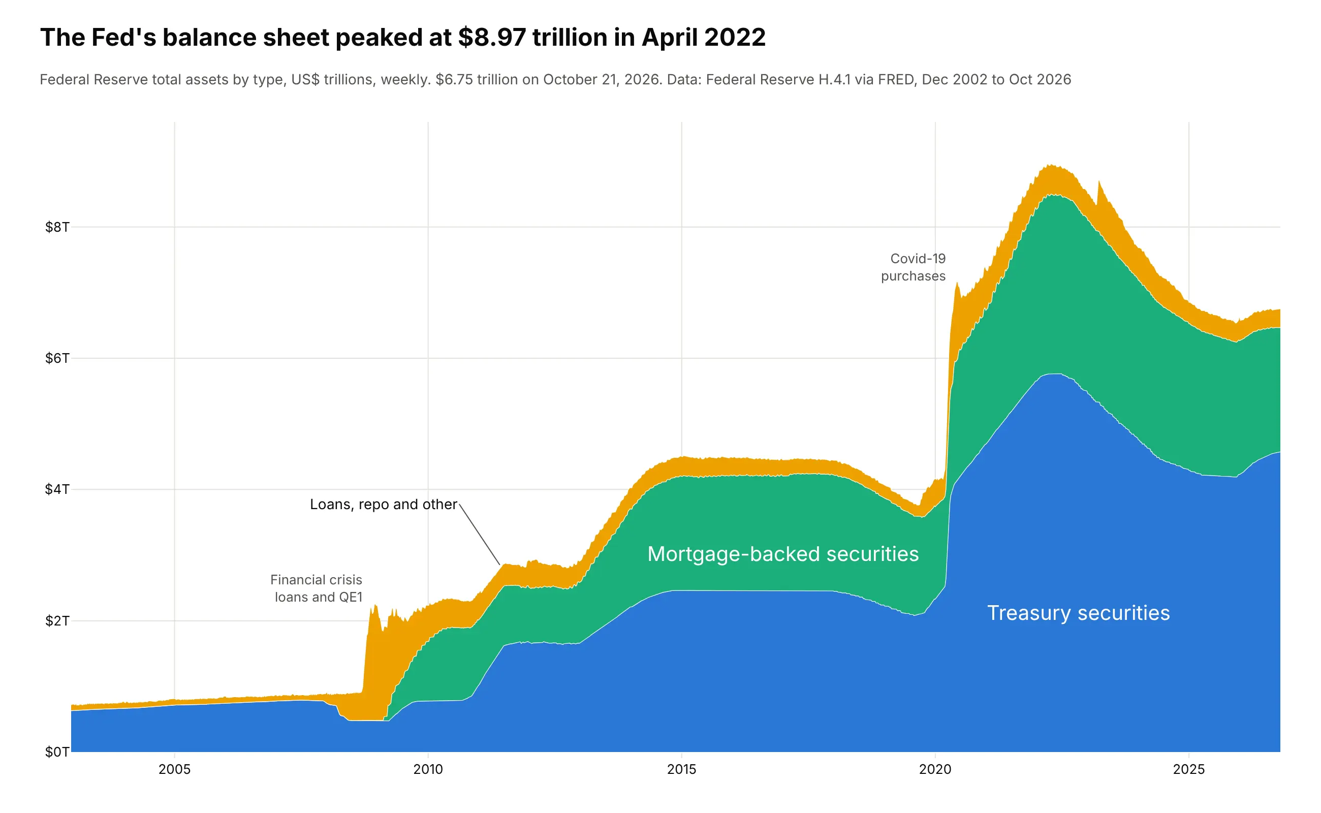
The Fed's balance sheet peaked at $8.97 trillion in April 2022 and was $6.75 trillion on October 21, 2026. Here readers ask "how big is it?" first, so this one keeps the zero baseline and a y axis: the same helper with baseline="zero". Data: Federal Reserve H.4.1 via FRED.

Tip: a thin top layer gets an outside label with a pointer instead of a label squeezed inside it.

5. What Americans died of, week by week

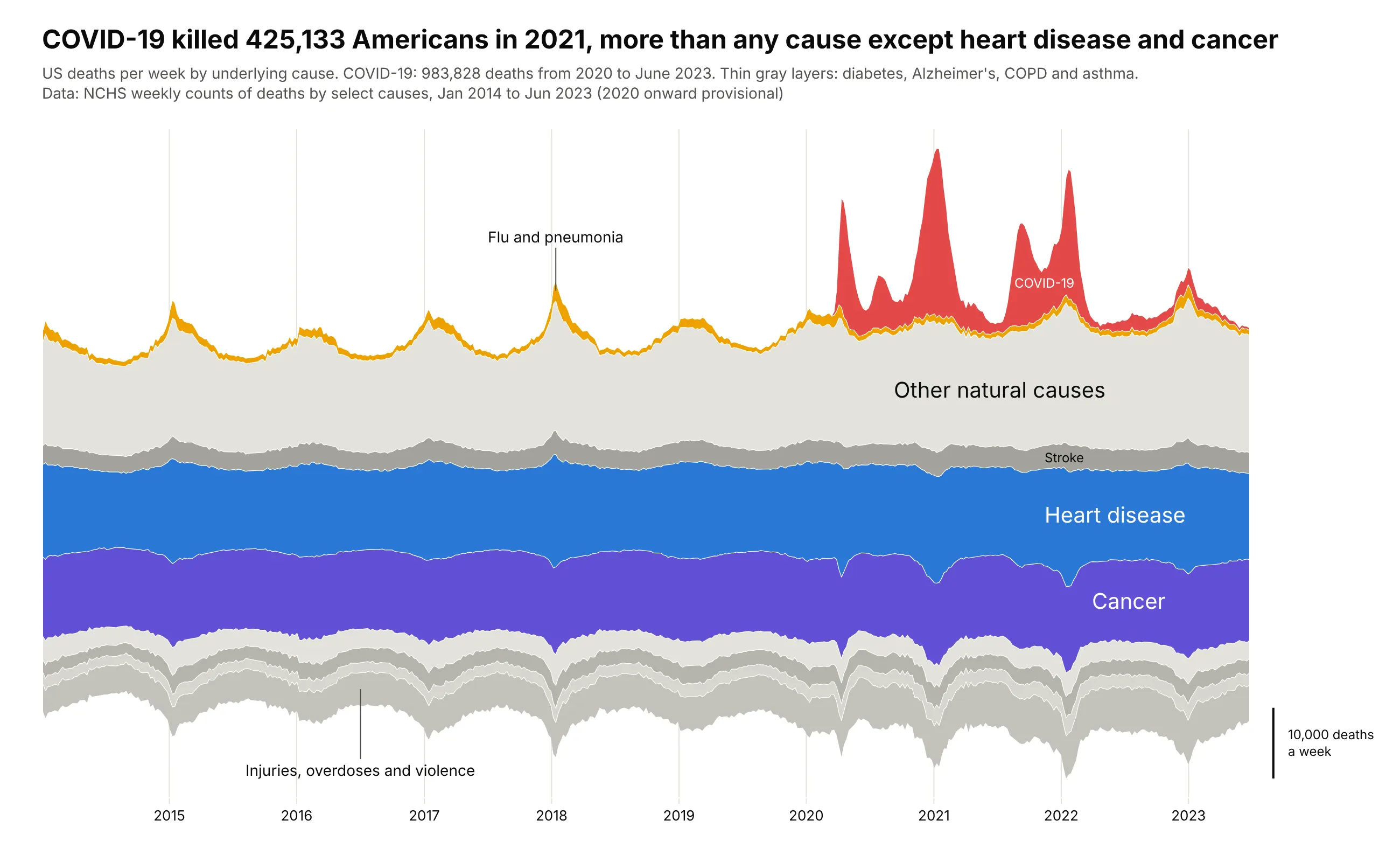
COVID-19 killed 425,133 Americans in 2021, more than any cause except heart disease (694,876) and cancer (604,296), and 983,828 from 2020 to June 2023. Before 2020 the biggest spikes are the winter flu seasons. Data: NCHS weekly counts of deaths by select causes.

Tip: the order is chosen by hand, with the steady causes in the middle and the spiky ones (COVID-19, flu) on the outside, so their spikes don't push every other layer up and down.

6. Who runs clinical trials

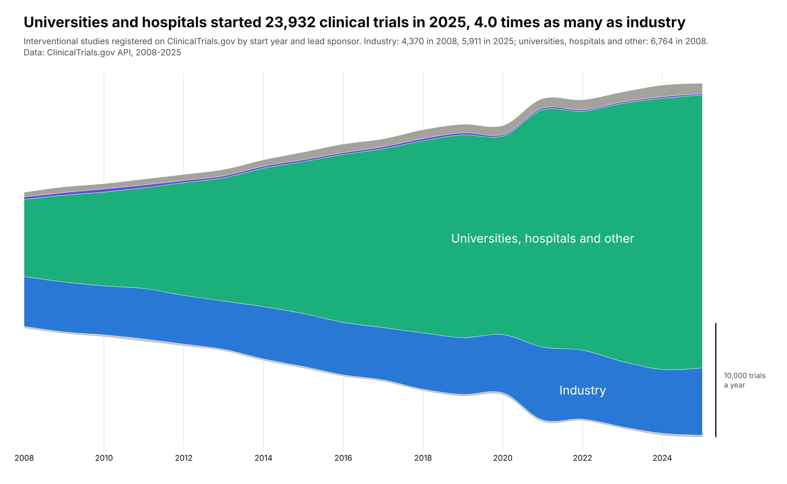
Universities and hospitals started 23,932 interventional trials in 2025, 4.0 times as many as industry (5,911). In 2008 the two were close: 6,764 and 4,370. Data: ClinicalTrials.gov API, interventional studies by start year and lead sponsor class.

Tip: with yearly points, splines (smoothing=1.0) make the layers easier to follow without changing any value at the data points.

7. Which GLP-1 drugs people read about

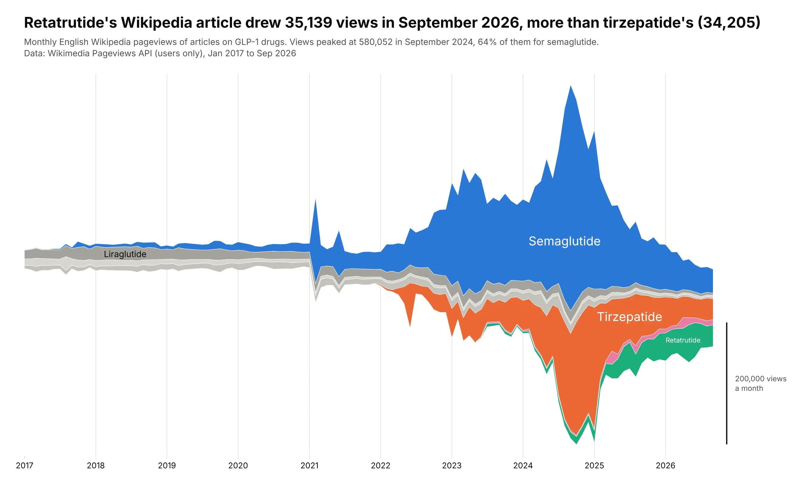
Readers of the GLP-1 articles peaked at 580,052 views in September 2024, 64% of them on semaglutide's. By September 2026 retatrutide's article drew 35,139 views, more than tirzepatide's (34,205). Data: Wikimedia Pageviews API, English Wikipedia, users only.

Tip: the inside-out order puts drugs that peaked early in the middle and lets the newest ones grow on the outside, where a new layer doesn't push the others around.

8. How computer science took over arXiv

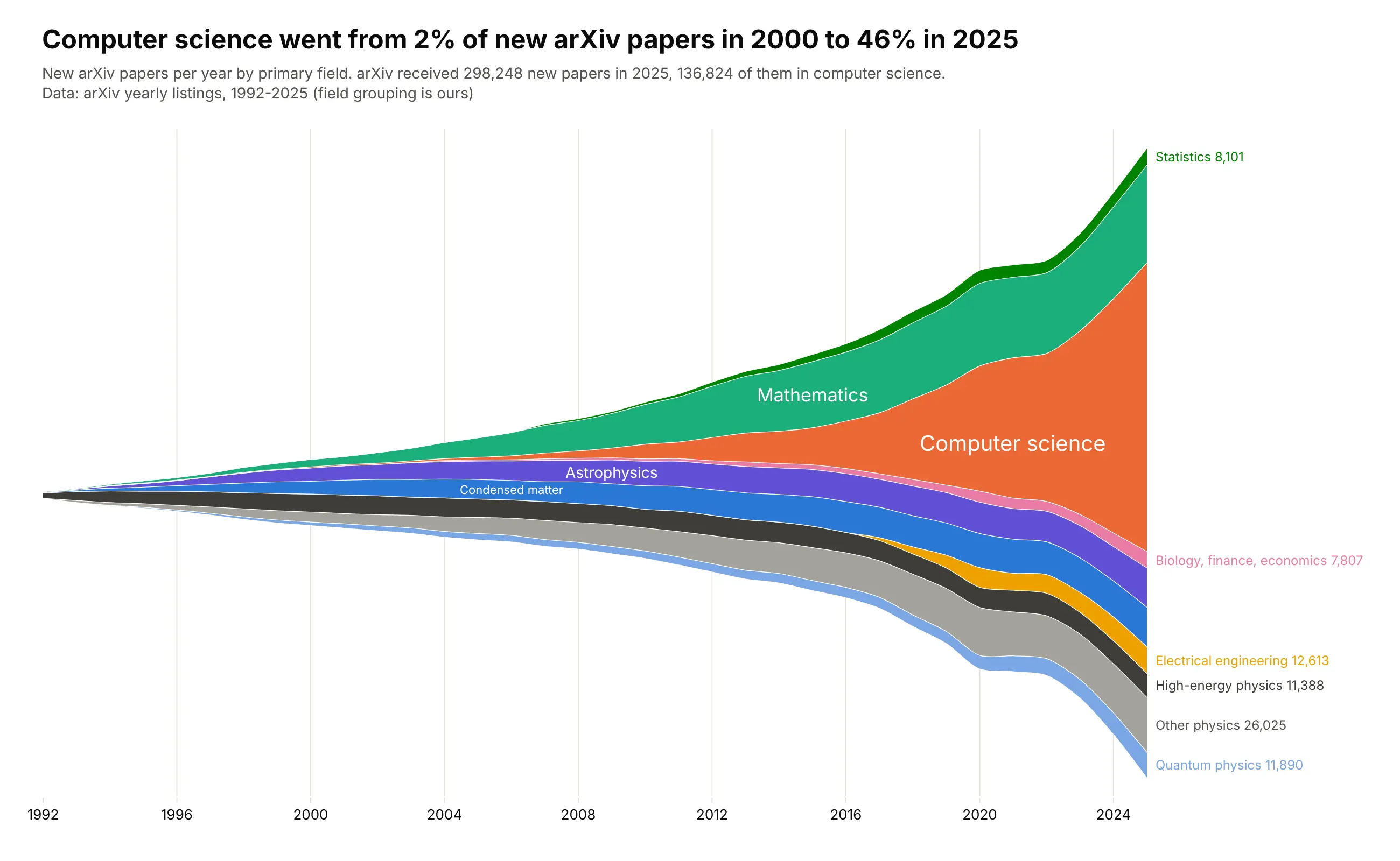
Computer science was 2% of new arXiv papers in 2000 and 46% in 2025, when arXiv received 298,248 new papers, 136,824 of them in computer science. The physics archives that founded arXiv still grow, from 27,126 papers in 2000 to 86,678 in 2025, just much more slowly. Data: arXiv yearly listings by primary archive (the field grouping is ours).

Tip: thin layers that can't hold a label inside get end labels in the right margin, at the middle of each layer in the last year.

9. The rise of boys' names ending in n

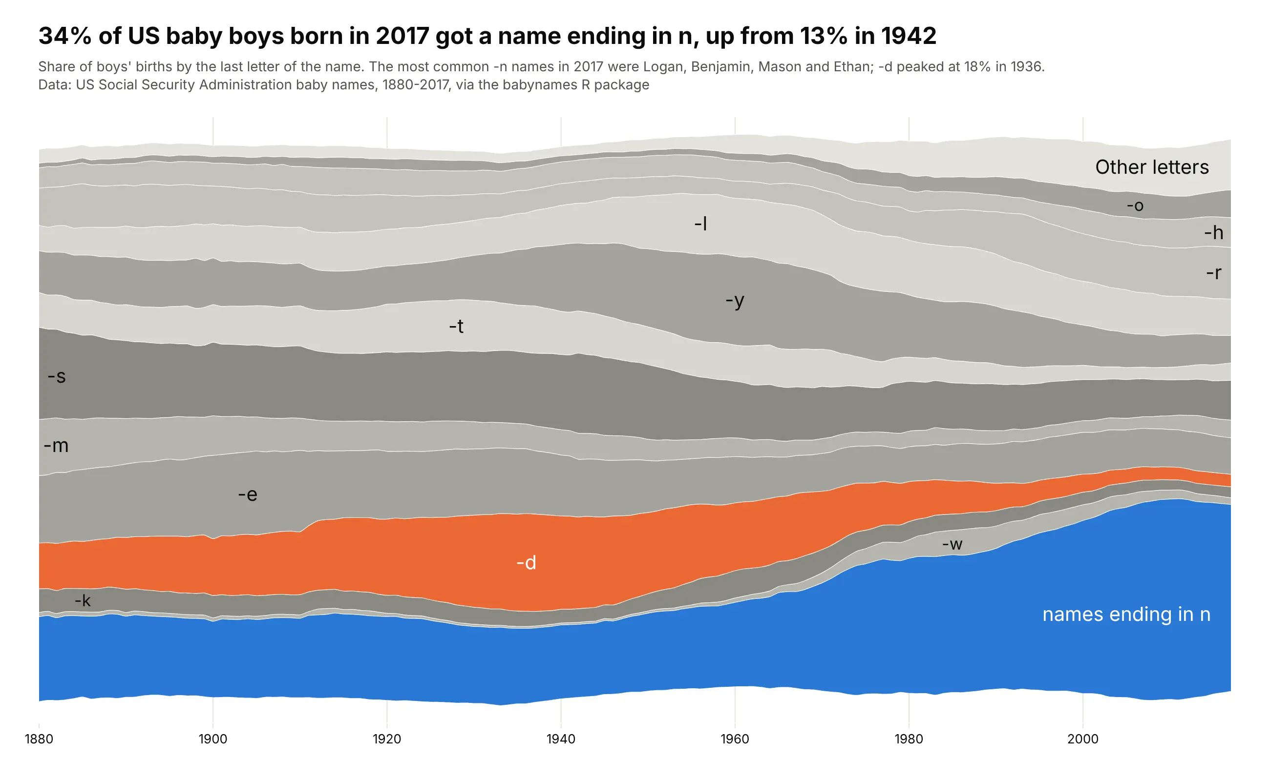
34% of US baby boys born in 2017 got a name ending in n, up from 13% in 1942. The -d names (Richard, Donald, David) peaked at 18% in 1936. Data: US Social Security Administration baby names, 1880-2017, via the babynames R package.

Tip: normalize=True gives every year the same height, so the chart is about the mix, not the number of births.

10. What MLB pitchers throw

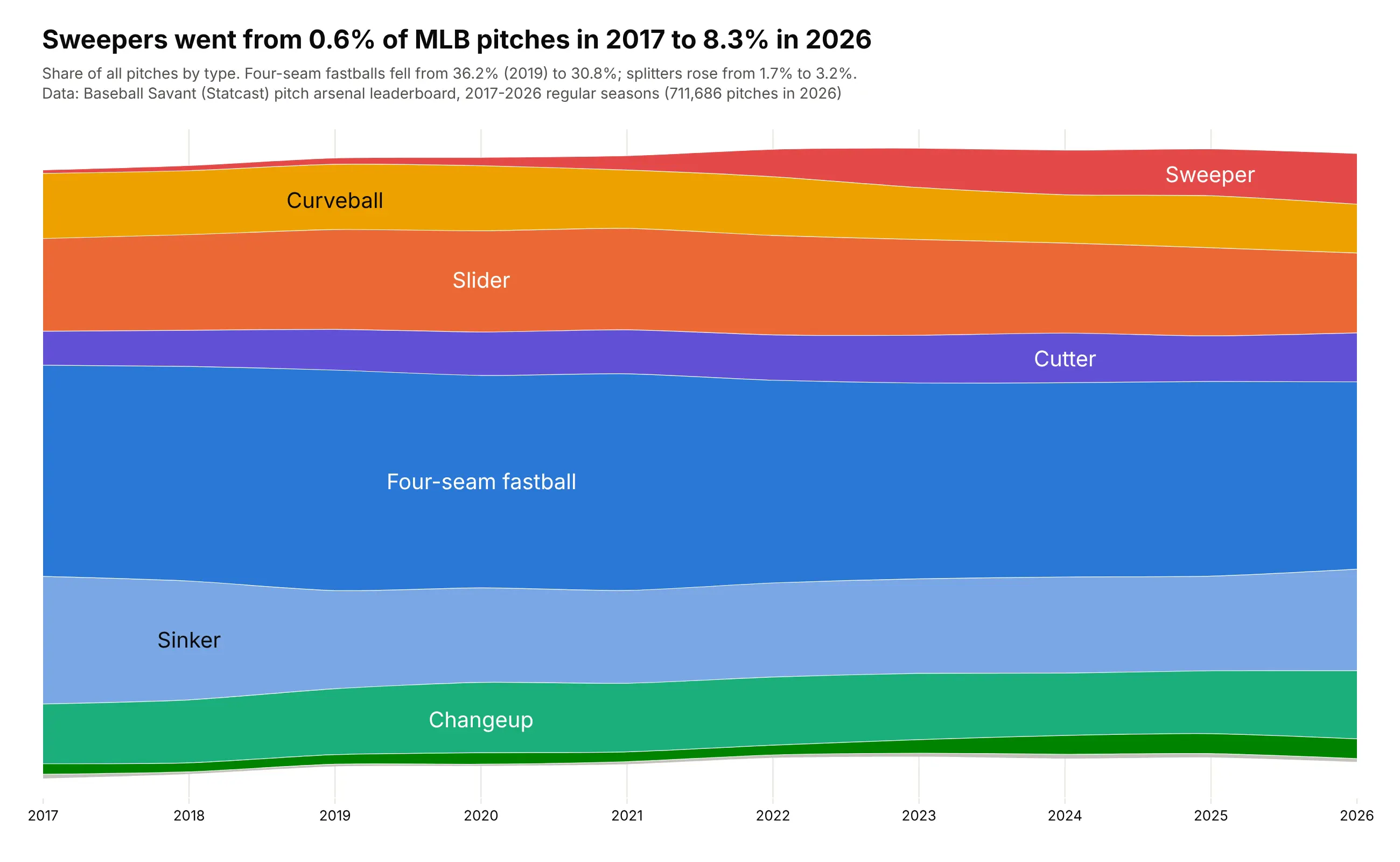
Sweepers went from 0.6% of MLB pitches in 2017 to 8.3% in 2026, while four-seam fastballs fell from 36.2% in 2019 to 30.8%. 2020's 60-game season had 262,443 pitches, 36% of 2019's, which would pinch every layer in a chart of counts. Data: Baseball Savant (Statcast) pitch arsenal leaderboard.

Tip: normalizing removes the short 2020 season from the picture, so the chart shows what pitchers threw, not how many games they played.

11. Which Olympic sports people read about, day by day

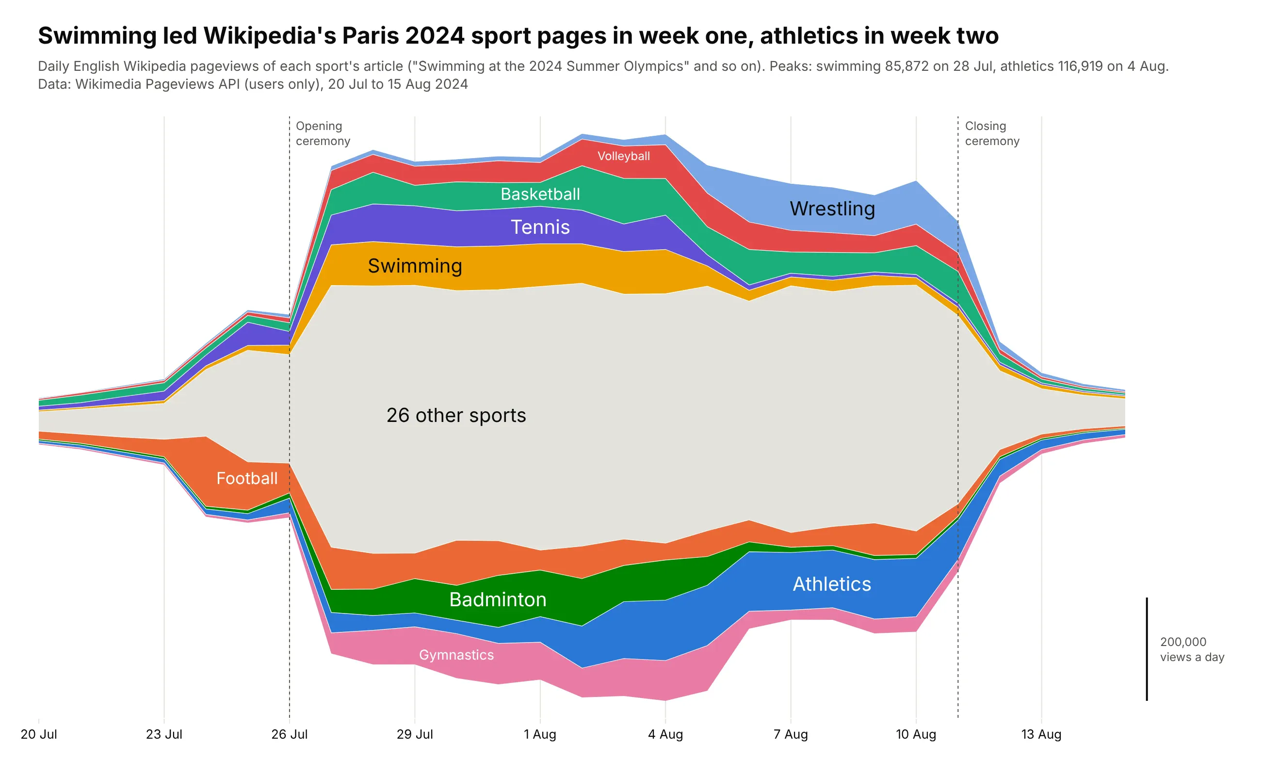
Swimming's Wikipedia article peaked at 85,872 views on 28 July 2024 and athletics at 116,919 on 4 August, so the Paris 2024 schedule shows up in what people read: each sport's layer swells while its events run and fades when they end. Data: Wikimedia Pageviews API.

Tip: the inside-out order puts the sports that peaked first in the middle, so the bulges follow the calendar of the Games from the center outward.