Ternary Plots - A Complete Guide

TL;DR

• A ternary plot draws items that split into three parts adding up to 100% as points in a triangle. Each corner is 100% of one part, so a point's position shows the whole split at once.
• Ternary plots are also known as ternary diagrams, ternary graphs, triangle plots and Gibbs triangles, and are similar to 100% stacked bar charts and scatter plots.
• Use one for many items with a three-way split (electricity mixes, vote shares, soil, diets, budgets) or for one item's split changing over time, drawn as a trail.
• Use 100% stacked bars instead when you have about a dozen items and readers need exact values, and a line chart when only one of the shares matters.
• Any coding agent can make one with Plotly in a minute. In Python it's px.scatter_ternary(df, a=..., b=..., c=...).

What is a ternary plot?

Ternary plots look like this:

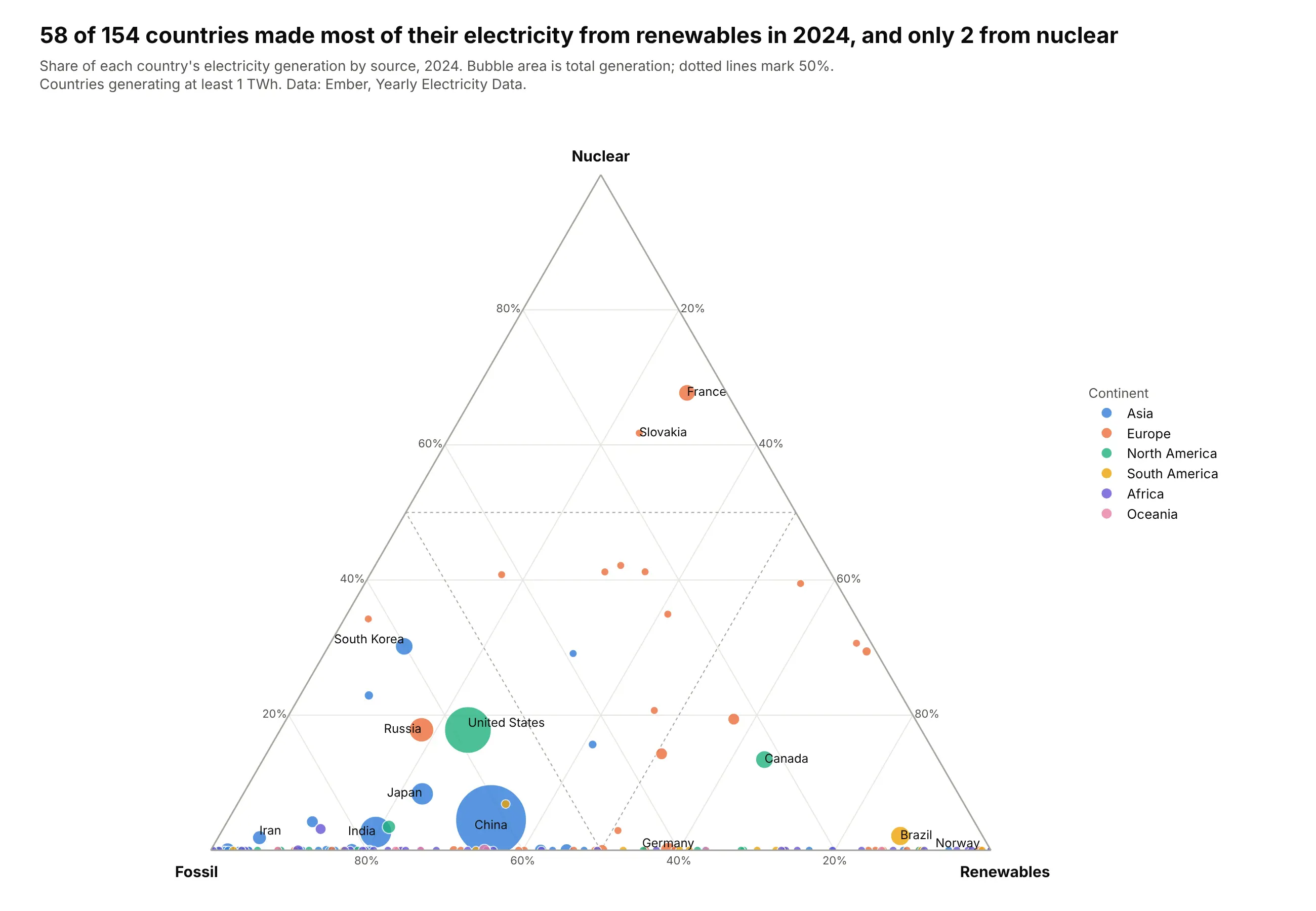
Data: Ember, Yearly Electricity Data, 2024.

How do you read a ternary plot? In the example above, notice these things:

• Each bubble is one country, placed by how its electricity splits between fossil fuels, nuclear and renewables. Its area is how much electricity it generated, which is why China is by far the biggest bubble.
• Each corner is 100% of one source, so the closer a bubble sits to a corner, the more of its power comes from that source. France sits high up toward the nuclear corner, while Brazil and Norway sit near the renewables corner at the bottom right.
• The bottom edge means no nuclear at all. Most countries generate no nuclear power, so they line up along that edge, from Saudi Arabia near the fossil corner to Norway at the renewables corner, with Germany at 59% renewables in between.
• The dotted lines mark 50%, which splits the triangle into regions where one source makes most of a country's power. Only France and Slovakia are above the nuclear line, while the United States and China are in the fossil region.
• To read exact values, follow the gridline through a point to the edge that carries its tick labels instead of dropping straight down to the nearest edge, because ternary gridlines meet the edges at 60 degrees.

It's often used for charts like these:

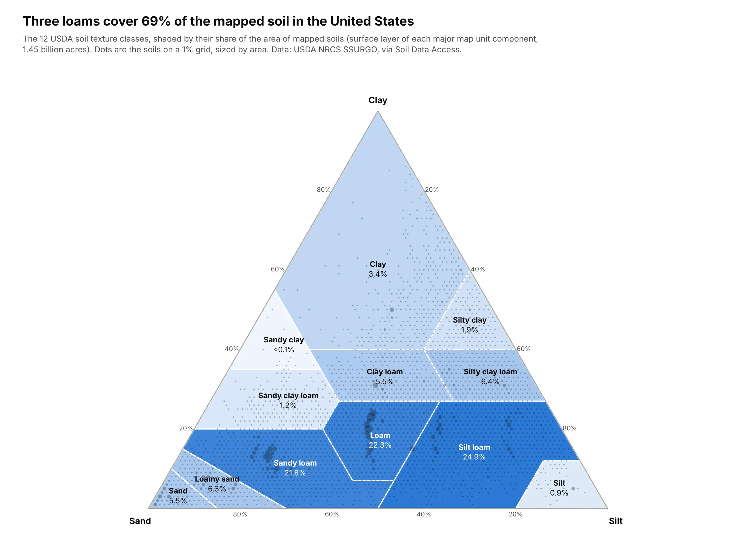
A classification drawn as regions. Soil scientists name soils by their share of sand, silt and clay, and weighted by area, three loams cover 69% of the mapped soil in the United States. Data: USDA NRCS SSURGO, via Soil Data Access (398,308 soil horizons, 1.45 billion acres).

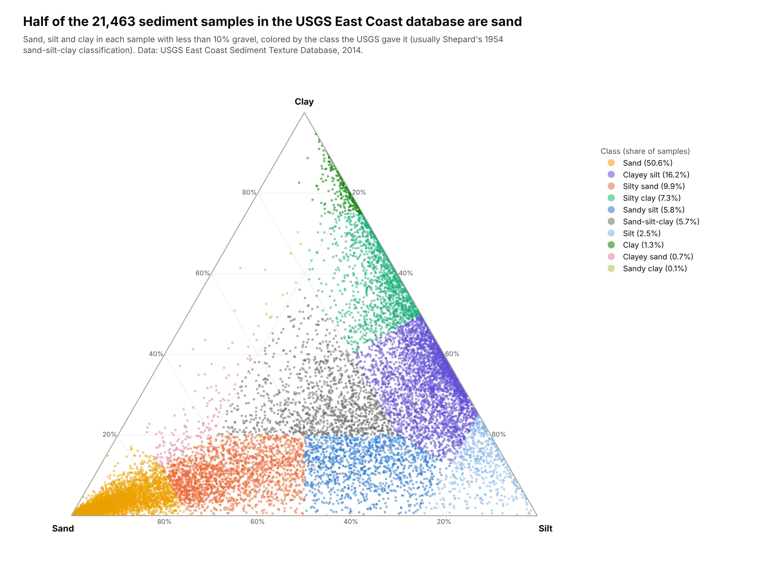
Sediment classified by grain size. Geologists sort seafloor and lake sediments by their share of sand, silt and clay, usually with Shepard's 1954 classification, and half of the 21,463 samples in the USGS East Coast database are sand. Data: USGS East Coast Sediment Texture Database (Poppe and others, 2014).

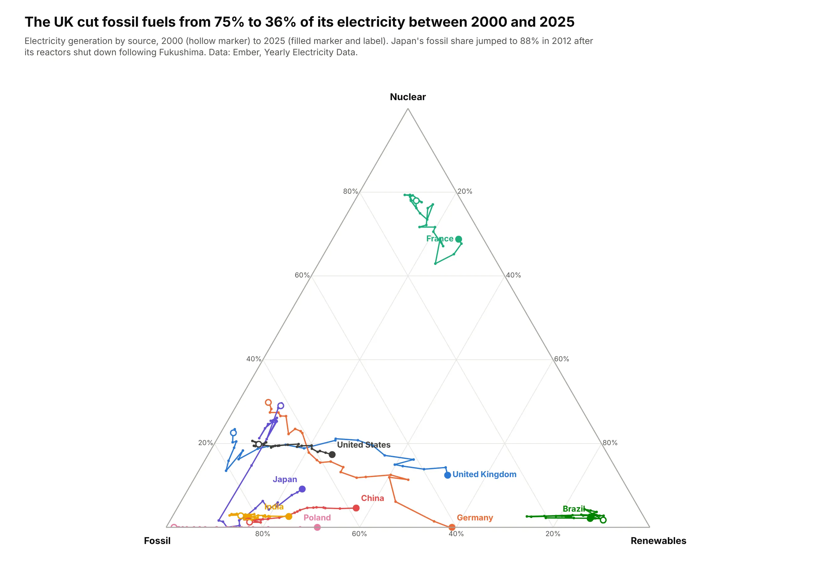
A split changing over time. The UK's trail shows fossil fuels falling from 75% to 36% of its electricity between 2000 and 2025, while Japan's jumps toward the fossil corner after its reactors shut down in 2012. Data: Ember, Yearly Electricity Data, 2000-2025.

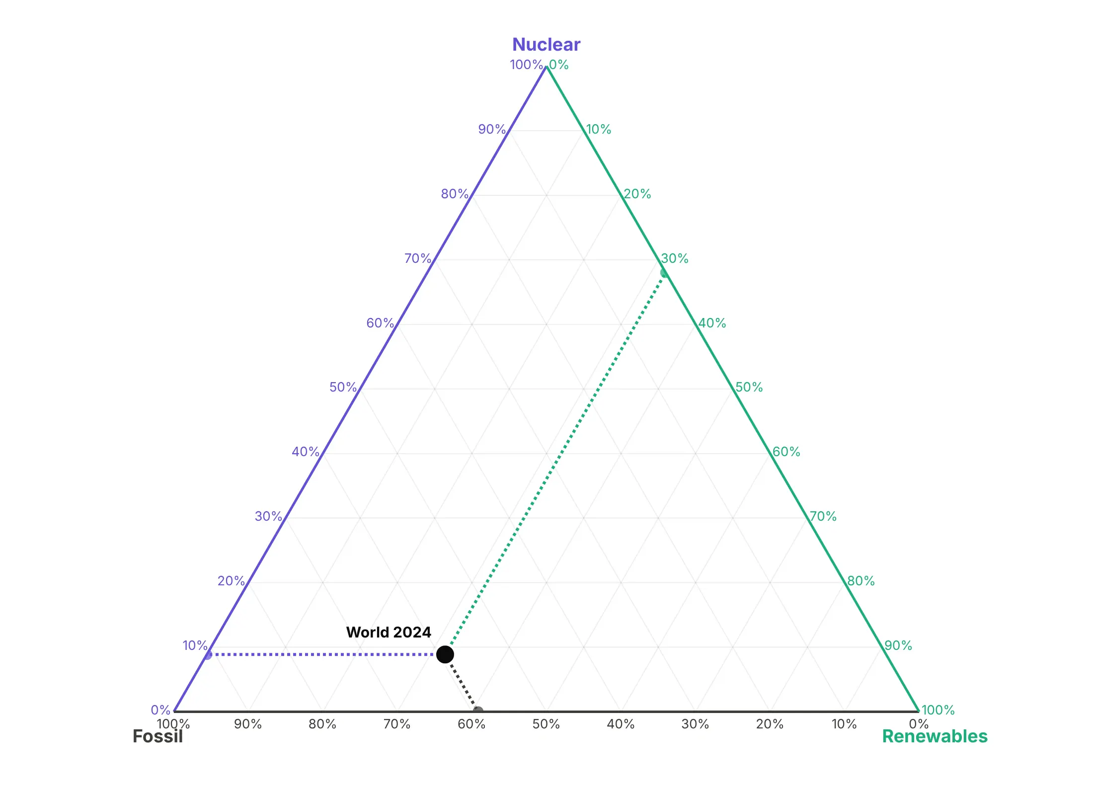
Reading exact values takes one more step. Follow the gridline through a point to the edge that carries the matching tick labels, as in this reading of the world's electricity in 2024 (59% fossil, 9% nuclear and 32% renewables):

A short history

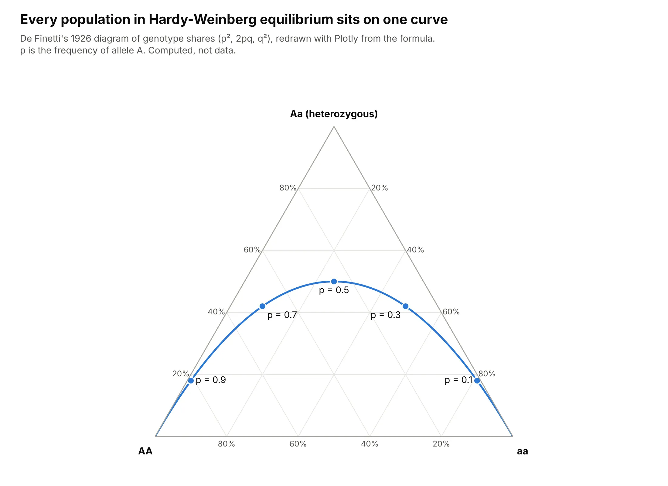
J. Willard Gibbs described a mixture of three substances as a point in an equilateral triangle in "On the Equilibrium of Heterogeneous Substances" (1876), which is why chemists still call it the Gibbs triangle and use it for three-component phase diagrams. In 1926 the mathematician Bruno de Finetti used the same triangle for genotype frequencies in a paper in Metron, and showed that every population in Hardy-Weinberg equilibrium falls on one curve:

Geologists later classified igneous rocks with Albert Streckeisen's QAP triangle (Streckeisen, 1976), soil scientists adopted the texture triangle shown above, and John Aitchison's work on compositional data (Aitchison, 1982) explained why shares that must add up to 100% need their own statistics.

Alternatives to a ternary plot

Here's the same electricity data for the 12 largest generators drawn six ways. Some are better for the question, some worse, some just different:

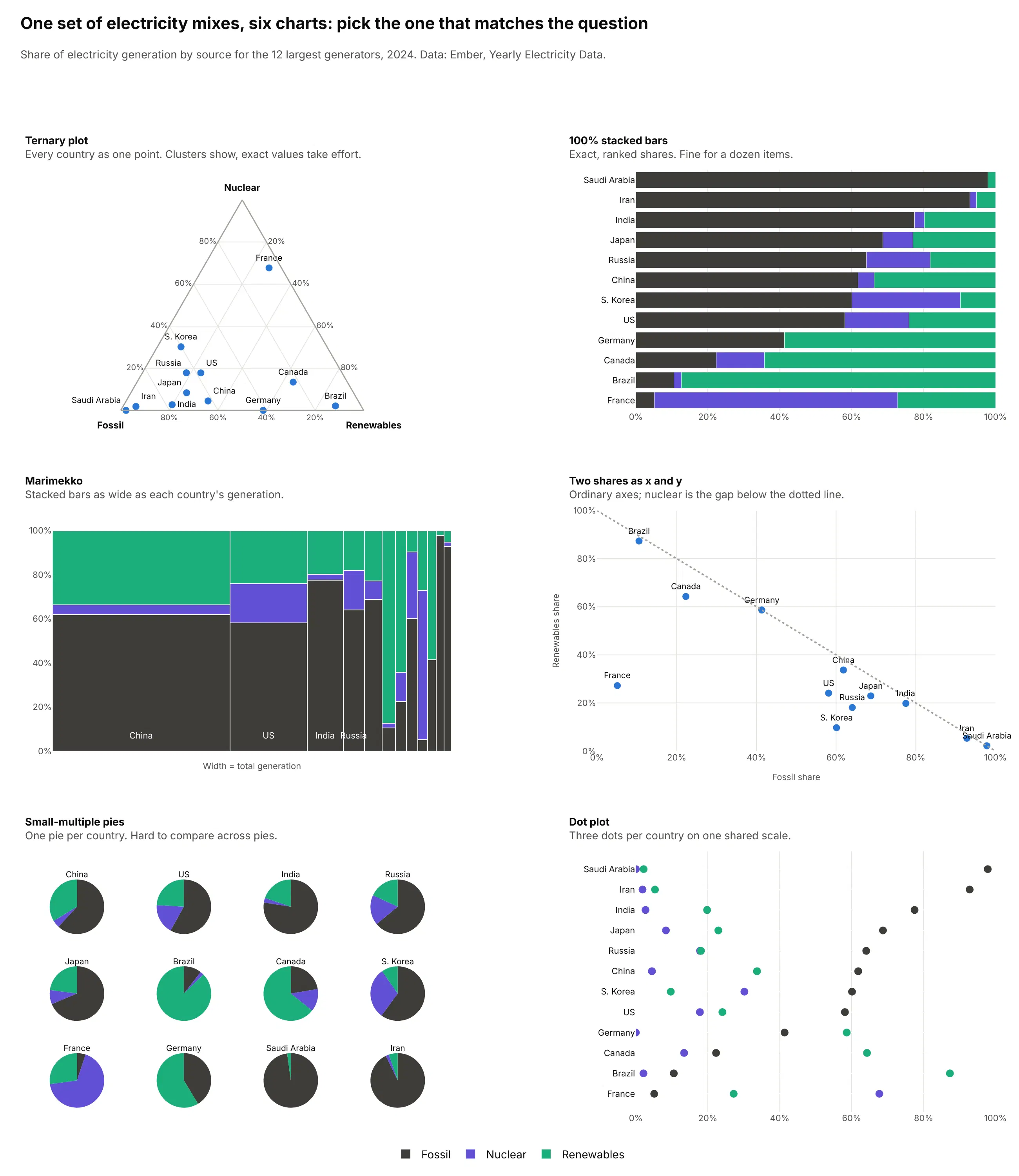
• 100% stacked bar chart (better for a dozen items and exact values). One bar per country, sorted by fossil share, makes it easy to read that Saudi Arabia gets 98% of its electricity from fossil fuels and France 5%. Past about 20 items the bars turn into a wall, and showing change over time needs one chart per item.
• Marimekko chart (better when size matters too). The same stacked bars with widths set by total generation show that China's 10,087 TWh dwarfs everyone else, which shares alone hide. See our Marimekko chart guide.
• Scatter plot of two shares (works too). Fossil against renewables uses ordinary x and y axes, and nuclear is the gap below the diagonal. It works when one of the three parts matters less than the others.
• Small-multiple pie charts (worse). One pie per country shows each split, but people compare angles across separate pies poorly, and 12 pies take far more space than 12 points.
• Dot plot (different). Three dots per country on one shared percent scale give exact values for every part, at the cost of the clusters a ternary plot shows.

The ternary plot is the only one of these that still works with 154 countries, or with one country's split over 25 years.

How to make a ternary plot

With AI

ChatGPT, Claude Code, GitHub Copilot, Cursor and other AI tools are excellent at writing Plotly code. Name Plotly in the prompt, say which part goes in which corner and what size and color mean, and list the checks you want:

The normalization check is worth keeping in every ternary prompt, because Plotly places any row in the triangle, even one with missing parts.

With Plotly Studio

Plotly Studio is a desktop app where you point an AI at a dataset and it builds charts and a Dash app around your questions. Ask for a ternary plot the same way:

Show a ternary plot of each country's electricity mix with nuclear at the top, fossil at the bottom left and renewables at the bottom right, in percent. Size the bubbles by total generation, color them by continent and label the 12 largest countries. Add a year slider.

Make a ternary plot in Python or JavaScript

This is the code AI tools write under the hood. In Python, Plotly Express takes one row per item and a column for each part, and divides each row by its total, so raw amounts work:

In JavaScript, plotly.js takes a scatterternary trace with the three parts in a, b and c. These are 2024 TWh from Ember:

To draw a region, such as a soil texture class or "more than half fossil", add another trace with the region's corners in a, b and c, mode: "lines" and fill: "toself". For a trail, sort by time and use mode: "lines+markers".

Share it

Every Plotly chart has a Share chart button (the cloud icon in its toolbar) that uploads it to Plotly Cloud and gives you a link. Only you can see it until you change its visibility.

For a live app, put the chart in a Dash app and publish it with the Plotly Cloud CLI. Coding agents can run these commands for you:

If your data has to stay in your own cloud or data center, publish to Dash Enterprise instead.

Dos and don'ts

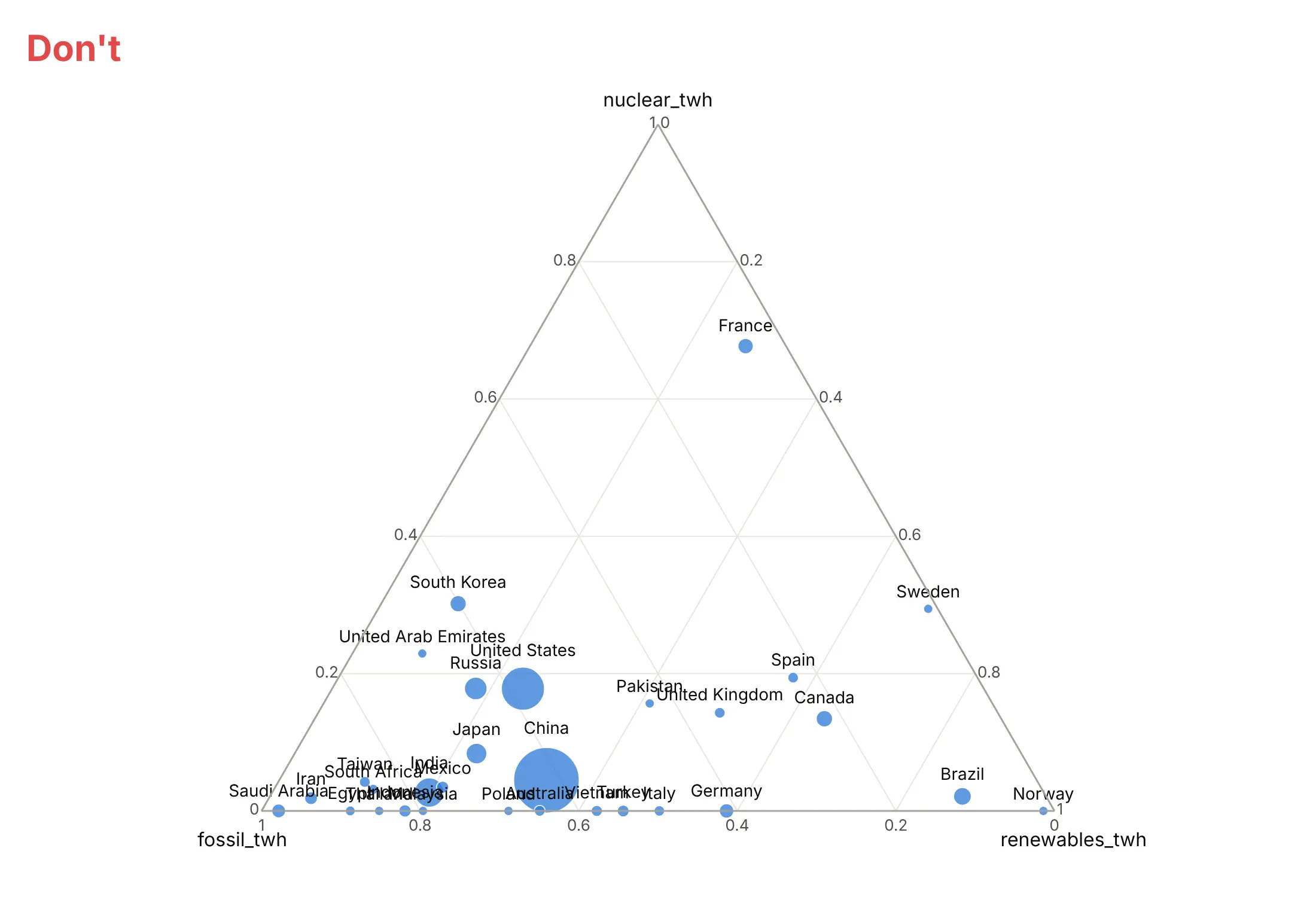
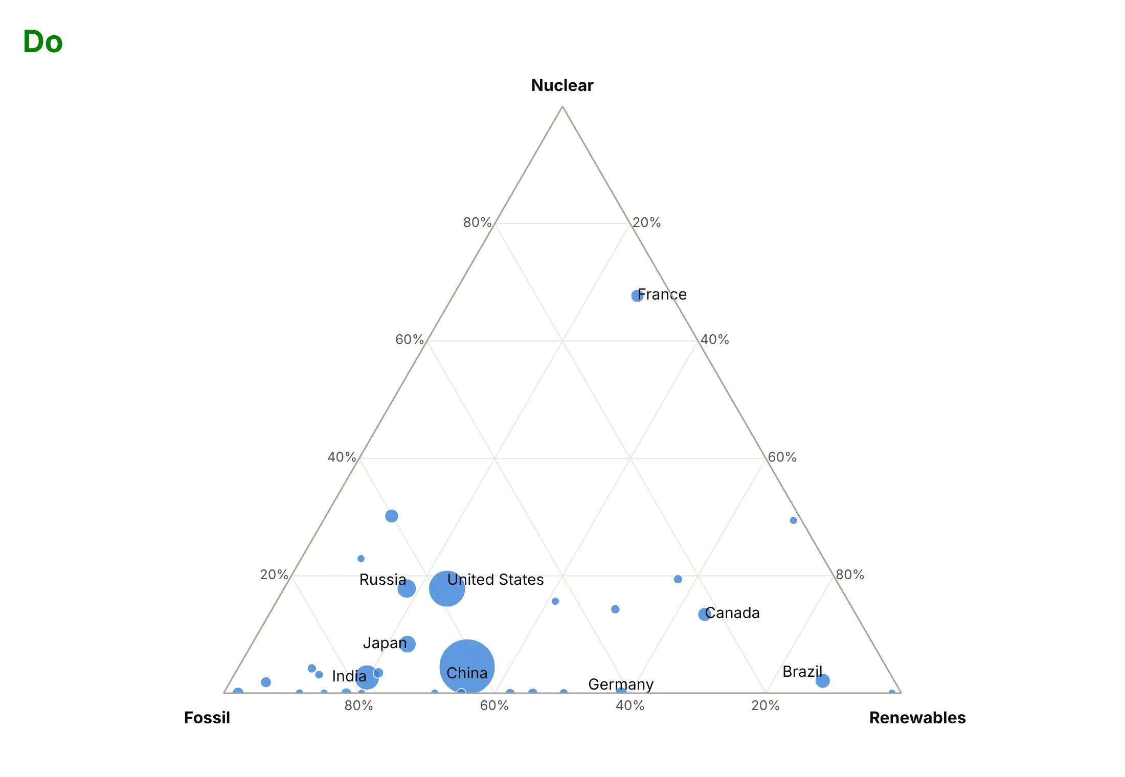
Most of the work on a published ternary plot is in the axes and the labels. Here are the 30 largest electricity generators of 2024 both ways, with the same bubbles and colors.

Don't leave column names such as nuclear_twh as axis titles, show the shares as fractions from 0 to 1, or force a label onto every point until they overlap:

Do show shares in percent with plain axis titles, and label only the countries readers will look for, leaving the rest to the hover:

Use size and color for one other thing

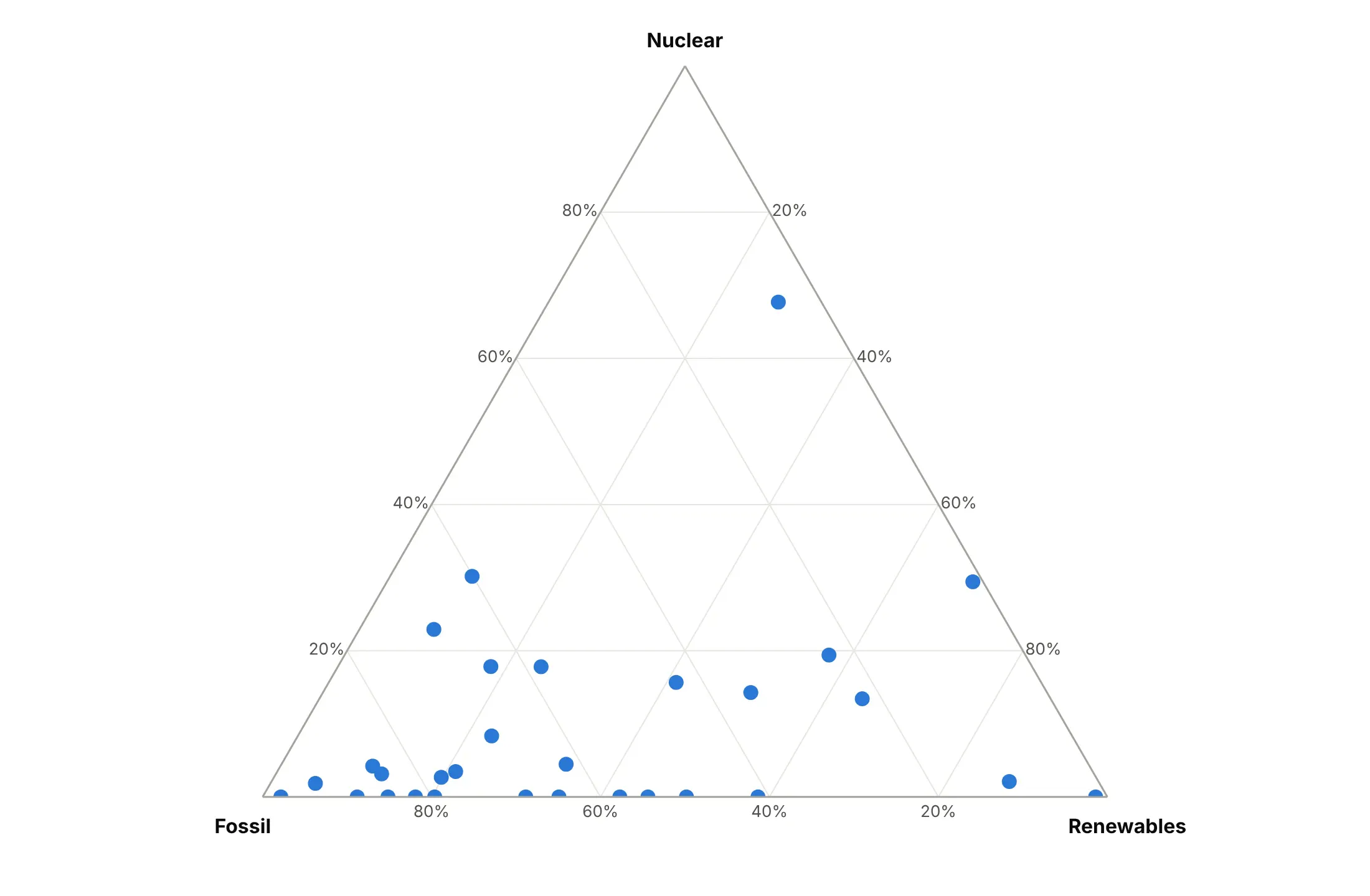
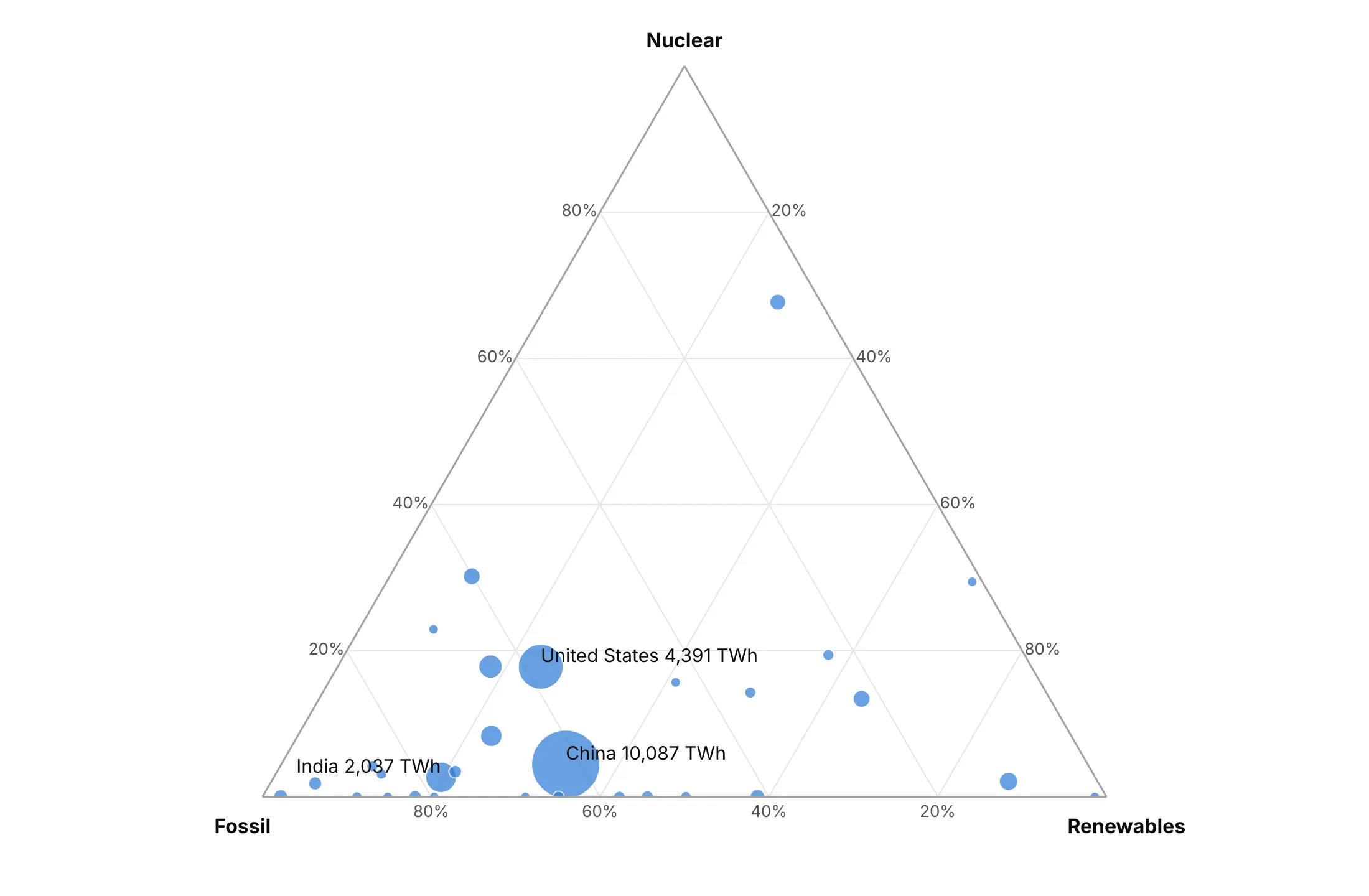
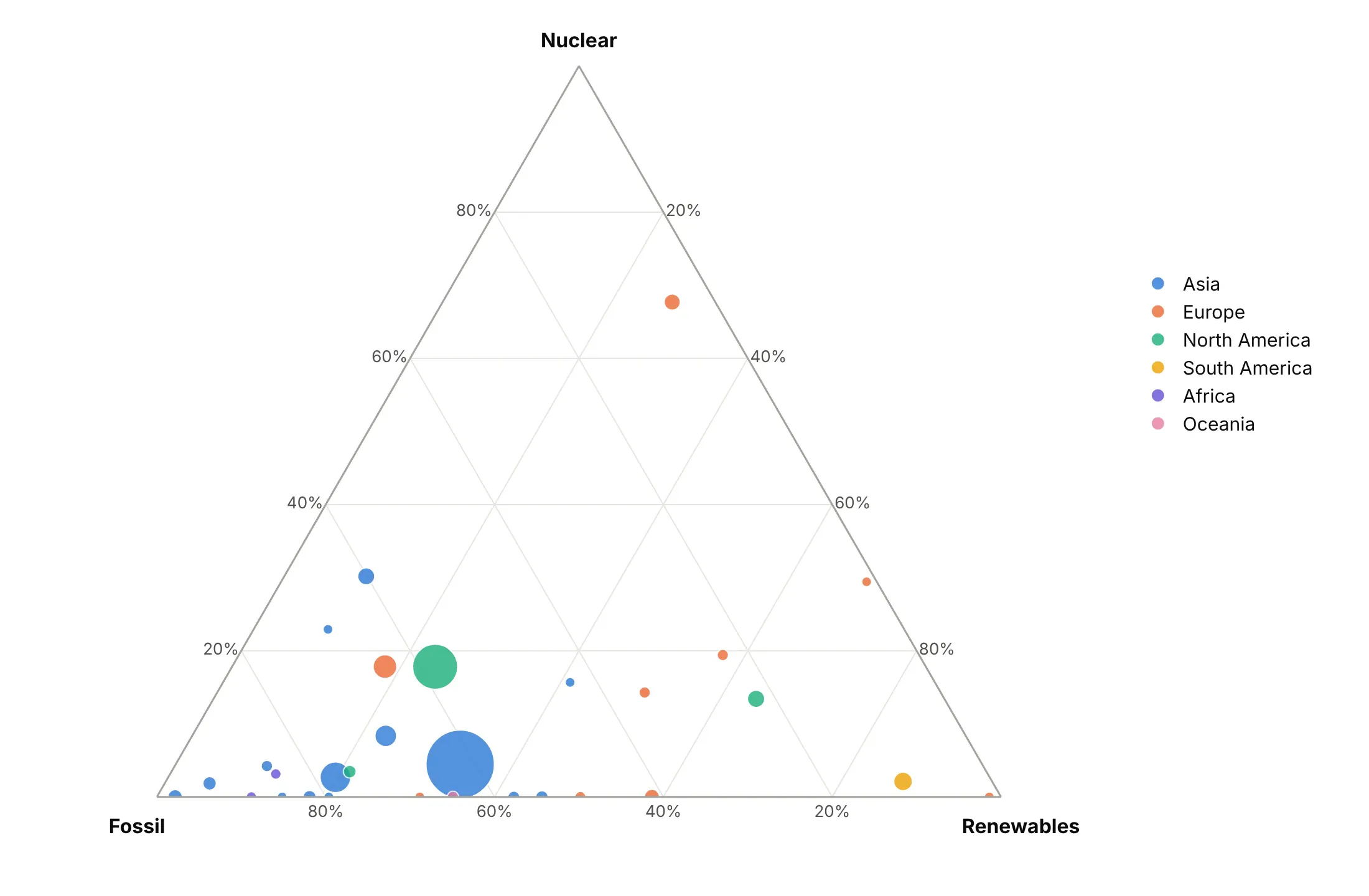
Position already shows the three shares, so size and color are free to say something else. Here are four options on the same data.

Plain points. Positions only, which is enough when every item matters equally.

Size by amount. Bubble area adds the total generation that shares hide, so China (10,087 TWh) and Norway no longer look alike.

Color by group. One hue per continent, which works for five or six groups and shows that most of Europe sits away from the fossil corner.

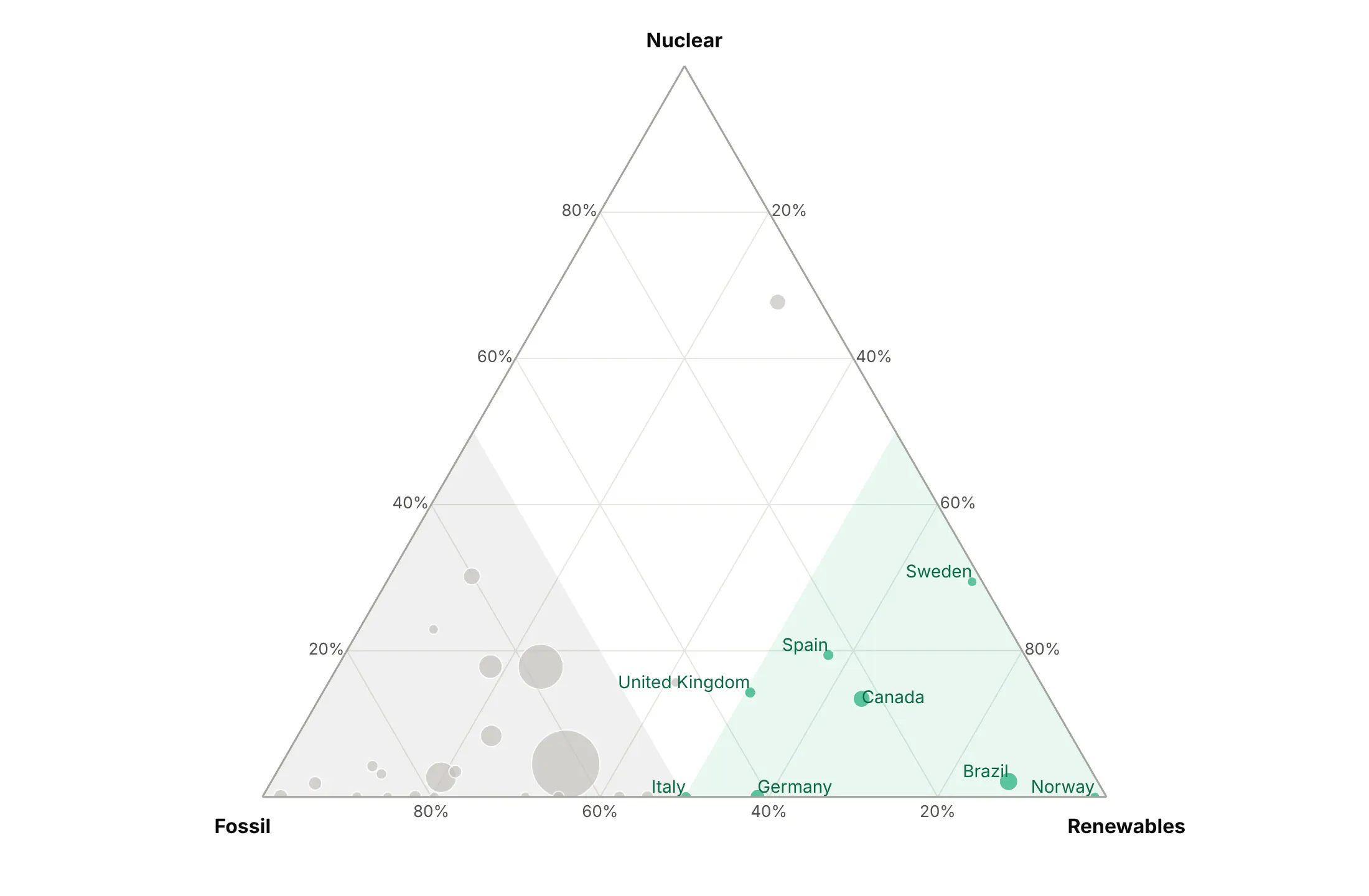
Highlight one story. The 8 countries that made most of their electricity from renewables are green, the rest gray, and the majority-fossil and majority-renewables regions are shaded.

Checklist

Do

• Write a title that states the takeaway, such as "27 US states made at least half their electricity from coal in 2001, and 5 did in 2025".
• Use sum=100 and ticksuffix="%" so ticks read 20% instead of 0.2.
• Name the axes in plain words, and color-code them when the audience is new to ternary plots.
• Zoom in with aaxis.min, baxis.min and caxis.min when the data uses a small part of the triangle, and say so in the subtitle.
• Draw reference lines and regions (50% lines, ties, classes) with a Scatterternary trace and fill="toself".
• Put all three values in the hover with hovertemplate.
• Use trails (mode="lines+markers") for change over time, with a hollow marker at the start.

Don't

• Label every point, because labels pile up along the edges where items with a zero share sit.
• Give every item its own color, because thirty colors can't be told apart.
• Read values by dropping a perpendicular to an edge; follow the gridlines.
• Plot three parts that don't add up to the whole without saying what was left out.
• Use a ternary plot for a few items that readers need to compare exactly.

Options to customize

These are the go.Scatterternary (and px.scatter_ternary, px.line_ternary) options and layout.ternary settings that matter most. The full list is in the Plotly ternary plots documentation.

1. a, b, c: the three parts for the top, bottom-left and bottom-right corners. Raw amounts are fine, Plotly normalizes them.
2. ternary.sum: the total the axes show (1 by default). Set it to 100 for percent ticks.
3. sum (trace): the total each point is normalized to; match it to ternary.sum when your values are already shares.
4. aaxis, baxis, caxis .title and .ticksuffix: axis titles and tick labels, in plain words and with %.
5. aaxis.min, baxis.min, caxis.min: raise a minimum to zoom into a smaller triangle when the data sits in one part.
6. color, linecolor, gridcolor, tickvals (on each axis): color-code axes for new readers and hide the corner ticks.
7. ternary.bgcolor, ternary.domain: the background and the triangle's place in the figure, for several triangles side by side.
8. mode: markers, lines, text or a combination; lines+markers for trails, text for labels.
9. marker.size, sizemode, sizeref: bubble size, to add the absolute amount that shares hide.
10. marker.color, colorscale, opacity: color by group or by a value such as the year, and transparency for dense data.
11. marker.symbol, marker.angleref: marker shape; angleref="previous" points arrows along a line for before and after.
12. fill="toself", fillcolor: fill a closed polygon for regions and classifications.
13. line.dash, line.width: reference lines such as ties and 50% lines.
14. text, textposition, cliponaxis: direct labels, and whether they can spill past the triangle.
15. hovertemplate, customdata: hover text with %{a}, %{b} and %{c}.
16. subplot: which ternary, ternary2 and so on a trace belongs to, for small multiples.

More ternary plot examples

Eleven more ternary plots built from real public data, each with its source, the technique that makes it work and a prompt to rebuild it.

1. US states moving off coal

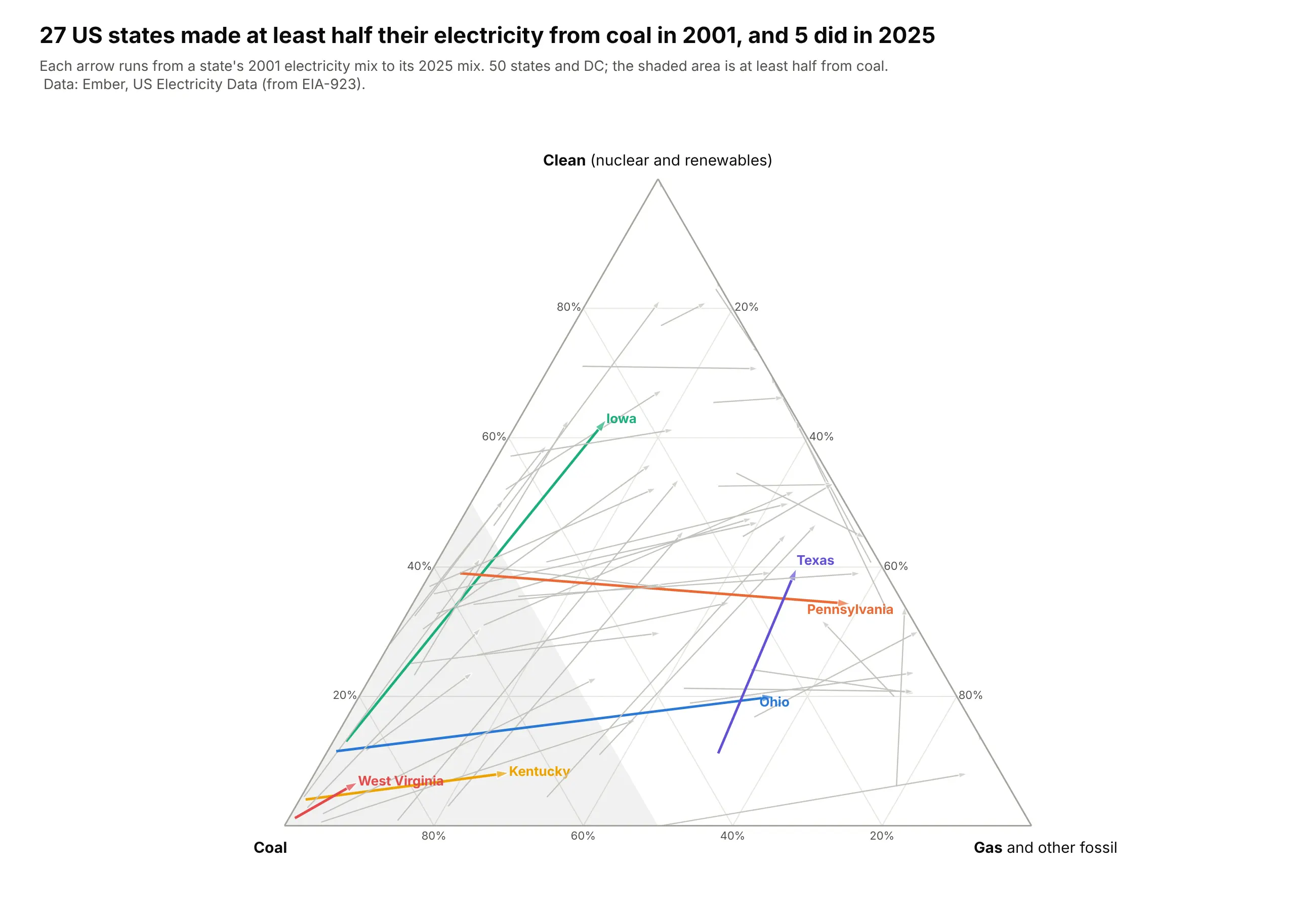
In 2001, 27 US states made at least half their electricity from coal, and in 2025, 5 did. The arrows show where they went: Iowa from 85% coal to 63% clean power, mostly wind, and Pennsylvania from 57% coal to 59% gas. Data: Ember, US Electricity Data (from EIA-923), 2001 and 2025.

Tip: marker.symbol=["circle", "arrow"] with angleref="previous" turns a two-point line into an arrow that points along the move.

2. Germany, month by month

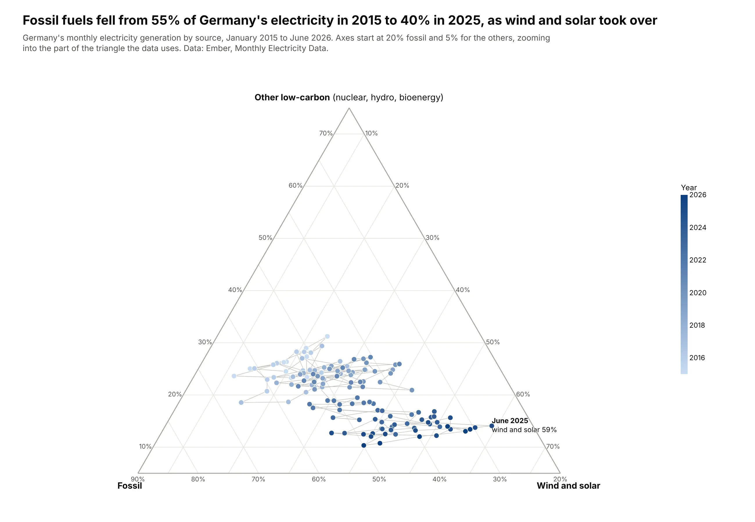
Fossil fuels made 55% of Germany's electricity in 2015 and 40% in 2025. Month by month, the cloud of 138 points drifts toward wind and solar, which peaked at 59% of generation in June 2025. Data: Ember, Monthly Electricity Data, January 2015 to June 2026.

Tip: setting aaxis.min, baxis.min and caxis.min zooms into a smaller triangle, and a sequential color by year turns 138 points into a visible drift.

3. Who holds US federal debt

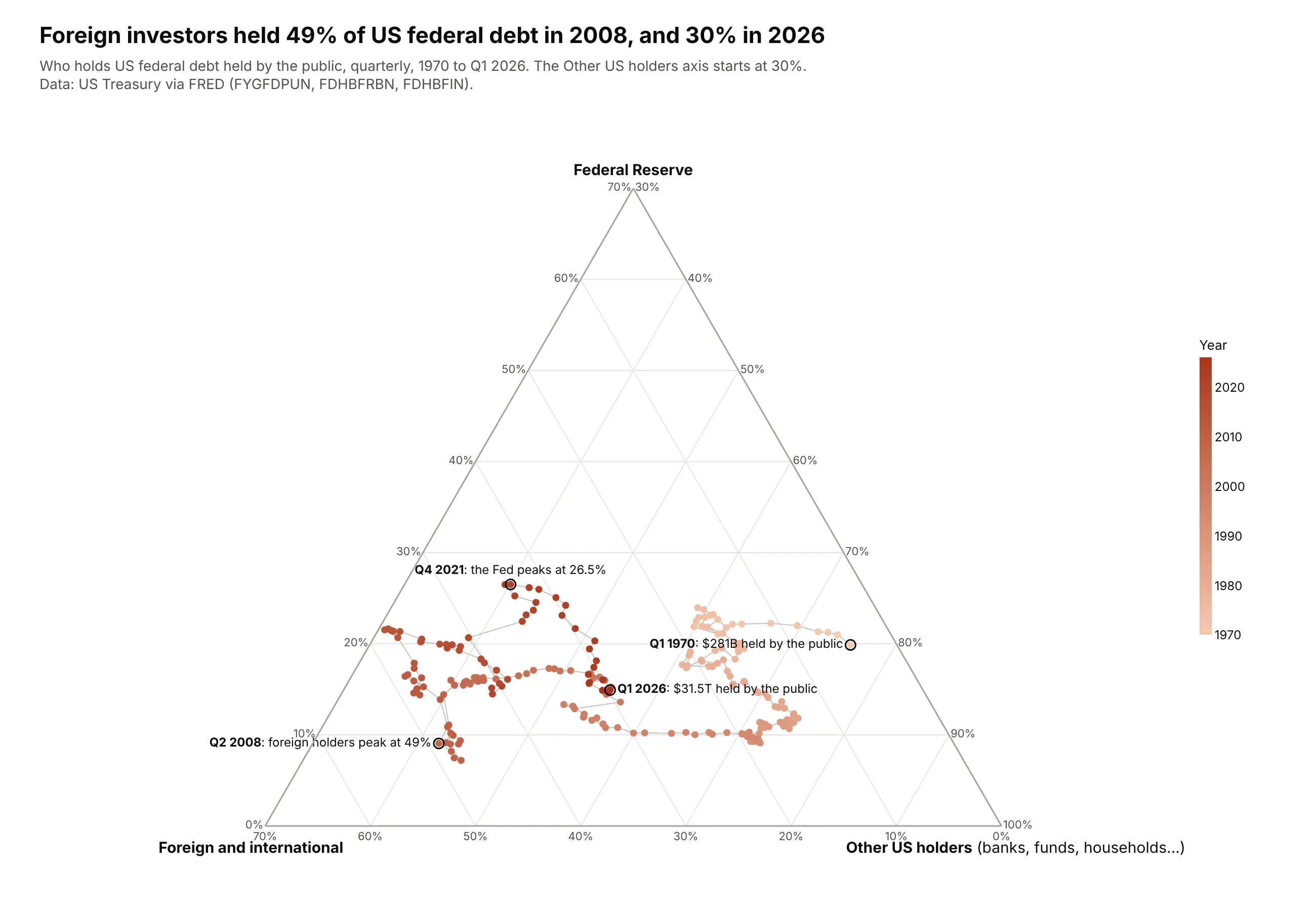
Foreign investors held 49% of US federal debt held by the public in 2008 and 30% in early 2026, while the debt grew from $5.3 trillion to $31.5 trillion. The Federal Reserve's share peaked at 26.5% in late 2021, after its pandemic purchases. Data: US Treasury via FRED (FYGFDPUN, FDHBFRBN, FDHBFIN), 1970-2026.

Tip: label only the turning points on a long trail with a hollow ring marker and text, and let the color scale carry the years.

4. What the rich and the rest own

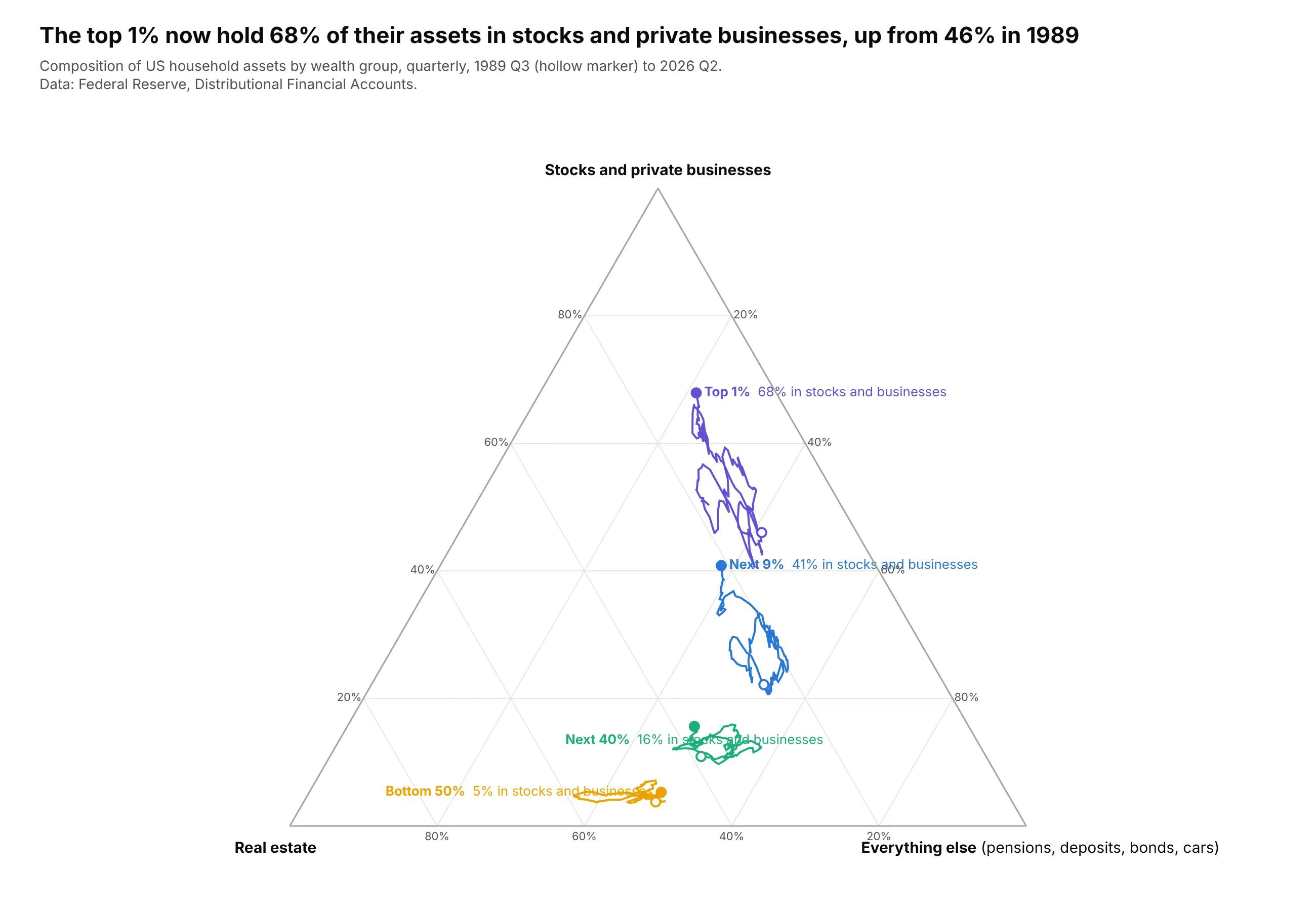
The top 1% of US households now hold 68% of their assets in stocks and private businesses, up from 46% in 1989. For the bottom half, that share is 5%, and real estate and everything else (cars, deposits, pensions) make up the rest. Data: Federal Reserve, Distributional Financial Accounts, 1989 Q3 to 2026 Q2.

Tip: four trails in four parts of the triangle tell a story by position alone, so labels can replace the legend.

5. The federal budget since 1962

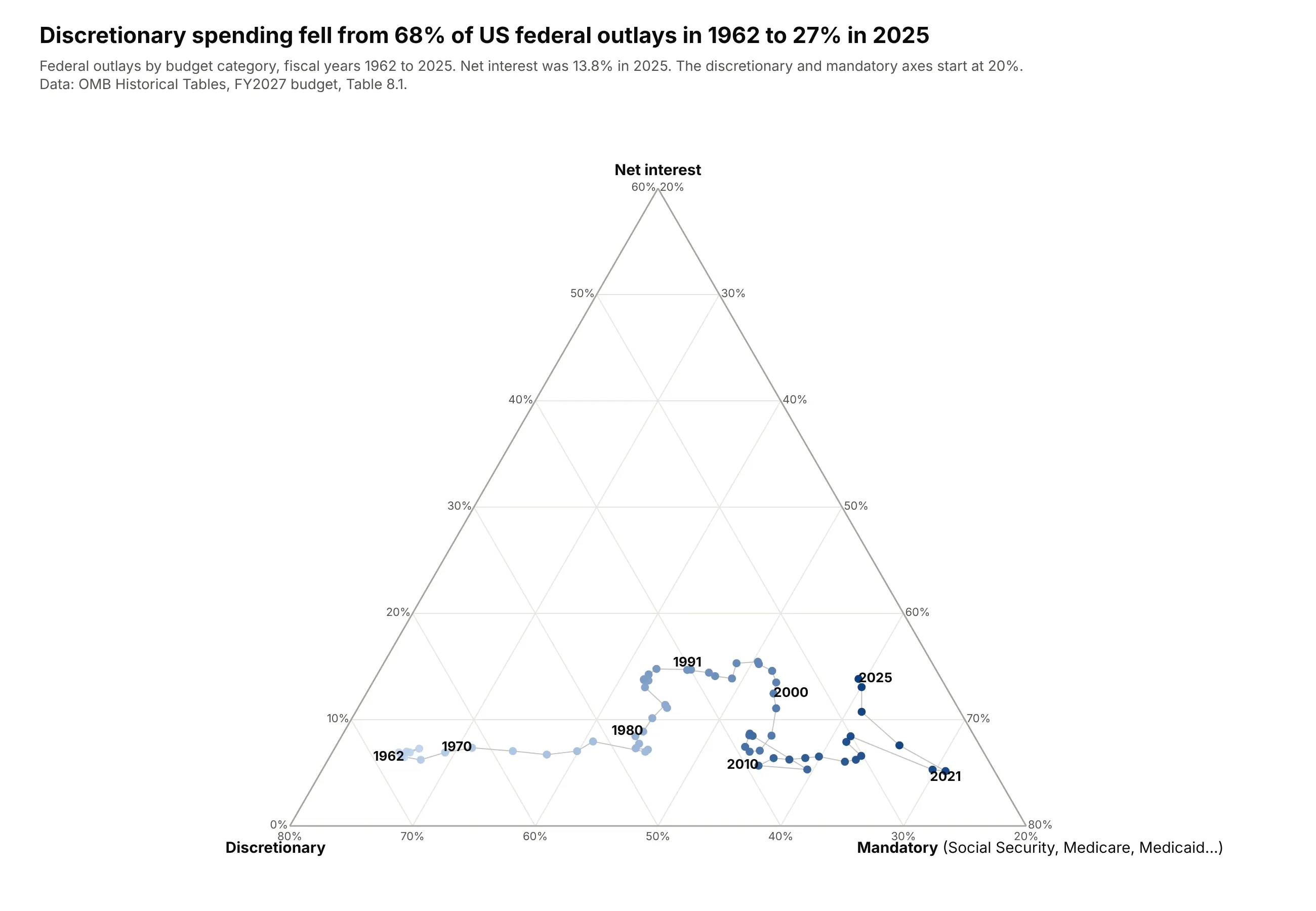
Discretionary spending fell from 68% of federal outlays in 1962 to 27% in 2025, as mandatory programs such as Social Security, Medicare and Medicaid grew to 59%. Net interest climbed back to 13.8% in 2025, from 5.2% in 2021. Data: OMB Historical Tables, FY2027 budget, Table 8.1.

Tip: year labels every decade along the trail are enough to anchor the timeline without a colorbar.

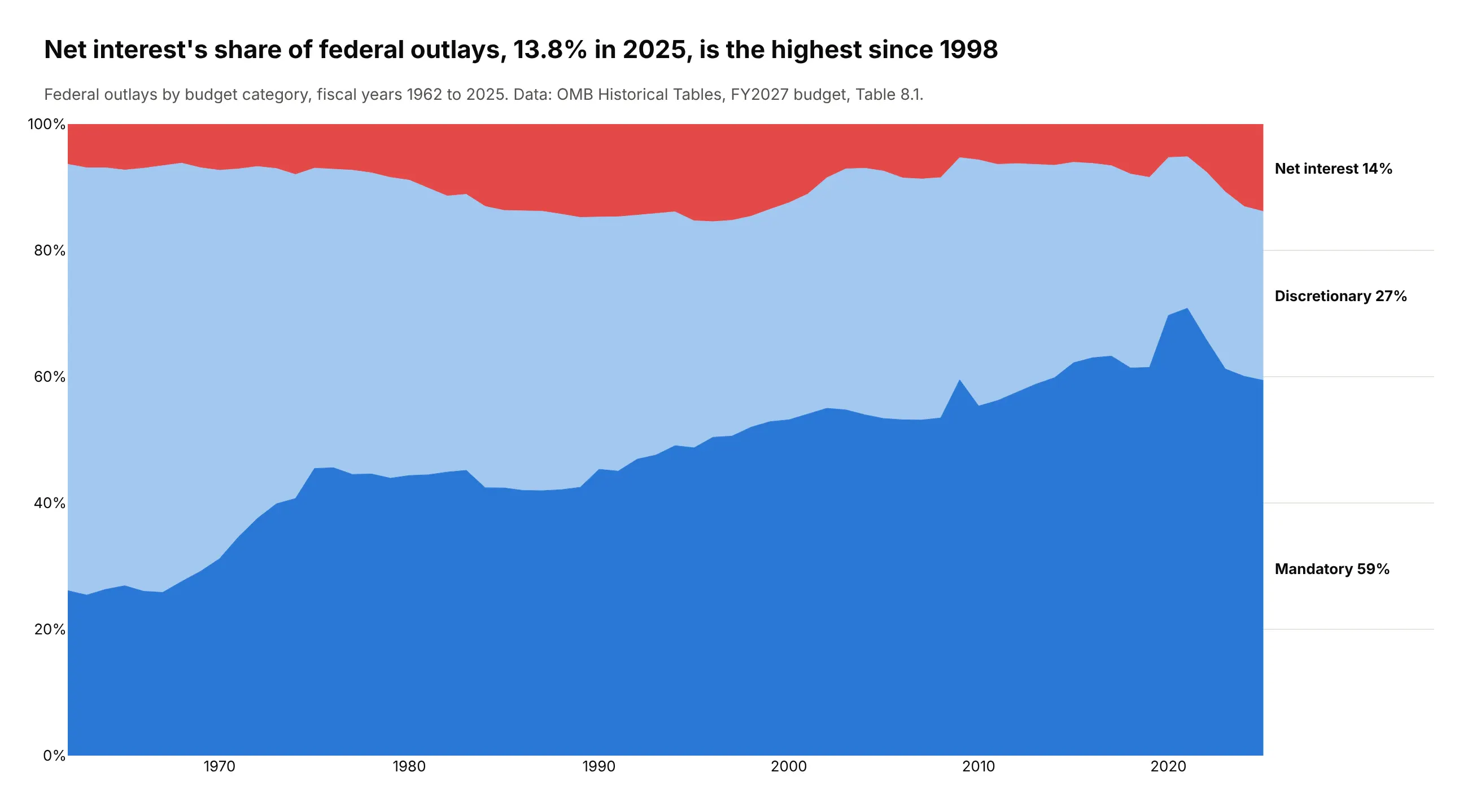
Another way to see it: a 100% stacked area chart reads more easily as a timeline and shows that net interest's 13.8% in 2025 is the highest share since 1998, but the thin interest band at the top is harder to compare across decades than its distance from the ternary plot's edge.

6. What people die of, by country income

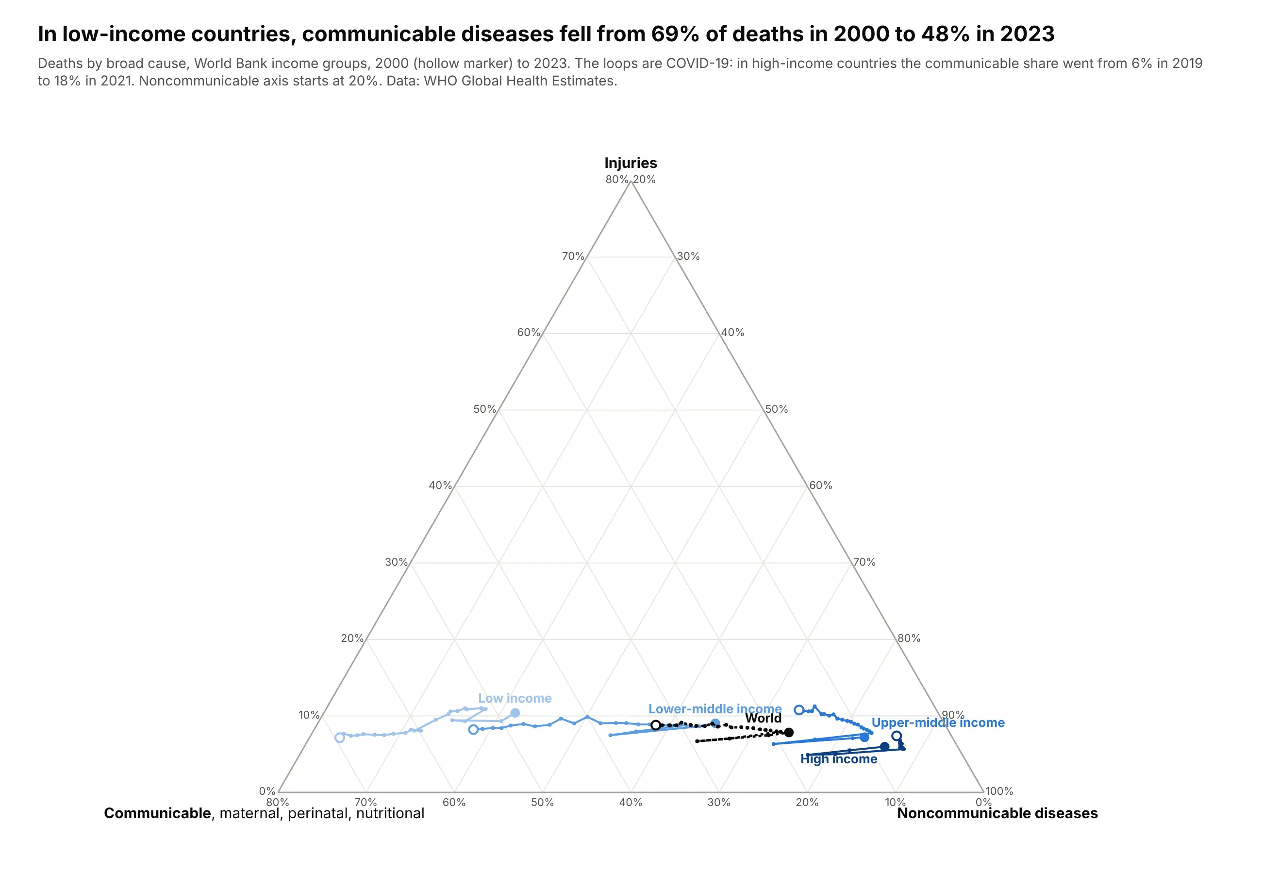
In low-income countries, communicable, maternal, perinatal and nutritional conditions fell from 69% of deaths in 2000 to 48% in 2023. The loops are COVID-19, which WHO counts as communicable: in high-income countries the communicable share went from 6% in 2019 to 18% in 2021. Data: WHO Global Health Estimates, 2000-2023.

Tip: an ordered blue scale for the income groups and a dashed black line for the world keep five trails readable without a legend.

7. Population aging since 1960

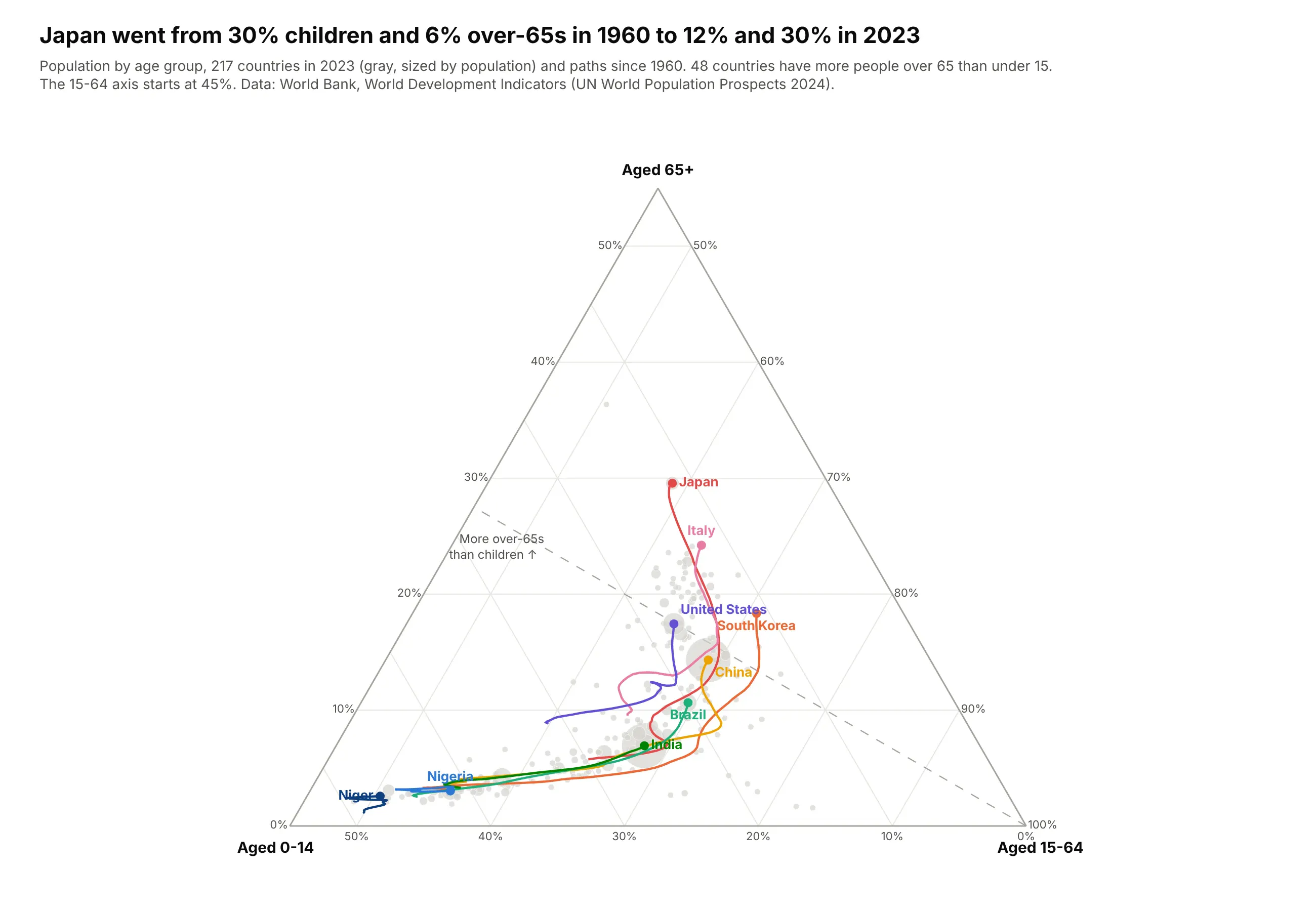
Japan went from 30% children and 6% over-65s in 1960 to 12% and 30% in 2023, and 48 countries now have more people over 65 than under 15. Nigeria and Niger have barely moved. Data: World Bank, World Development Indicators (UN World Population Prospects 2024), 1960-2023.

Tip: gray bubbles for every country in the latest year give the trails context without competing with them.

8. What 7,244 foods are made of

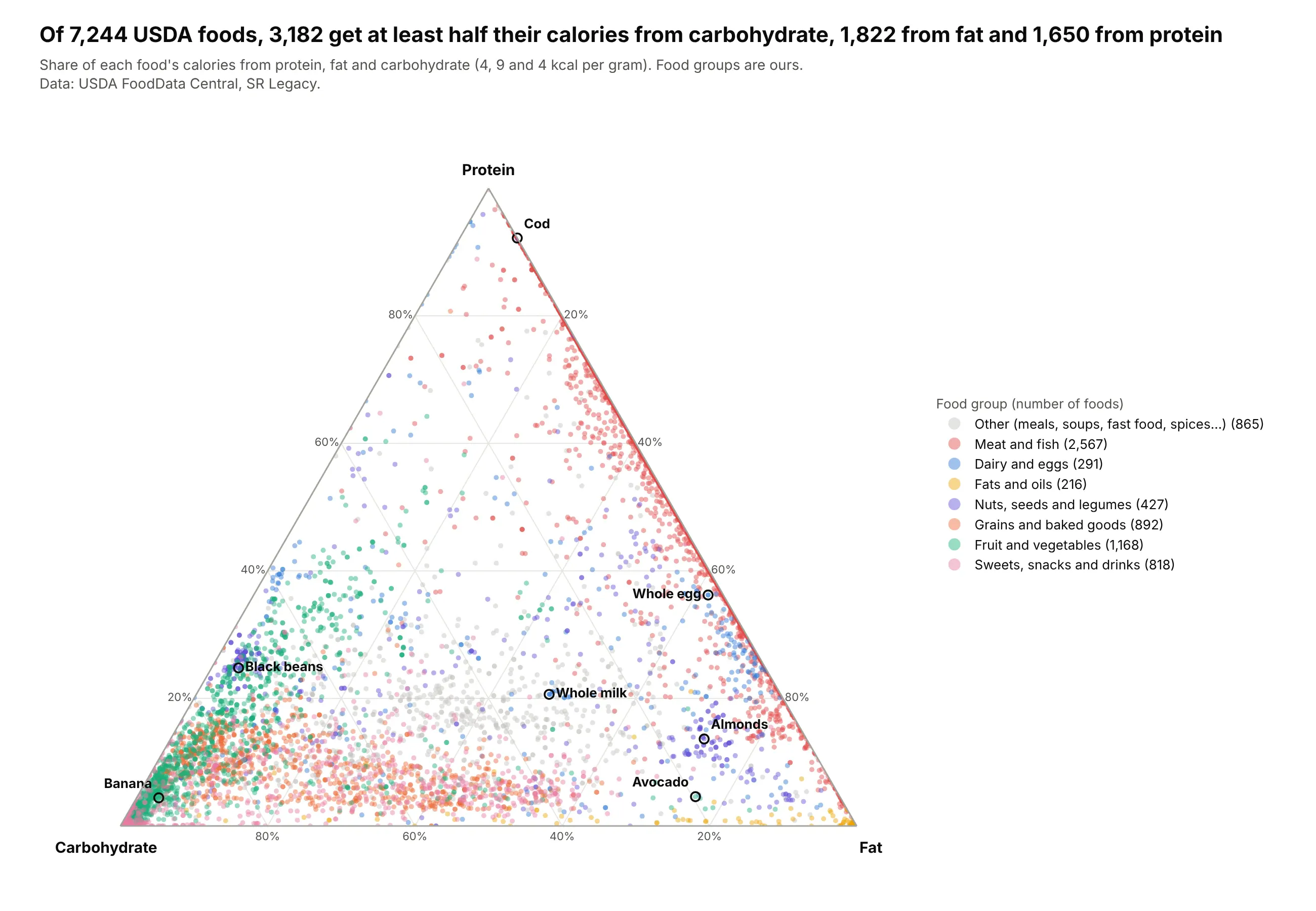
Of 7,244 foods in USDA's SR Legacy database, 3,182 get at least half their calories from carbohydrate, 1,822 from fat and 1,650 from protein. Meat and fish line the protein-fat edge with almost no carbohydrate, and cod is 92% protein. Data: USDA FoodData Central, SR Legacy.

Tip: small markers with opacity=0.45 turn overlap into density, so 7,244 points still read as shapes.

9. The shape of big pharma's pipelines

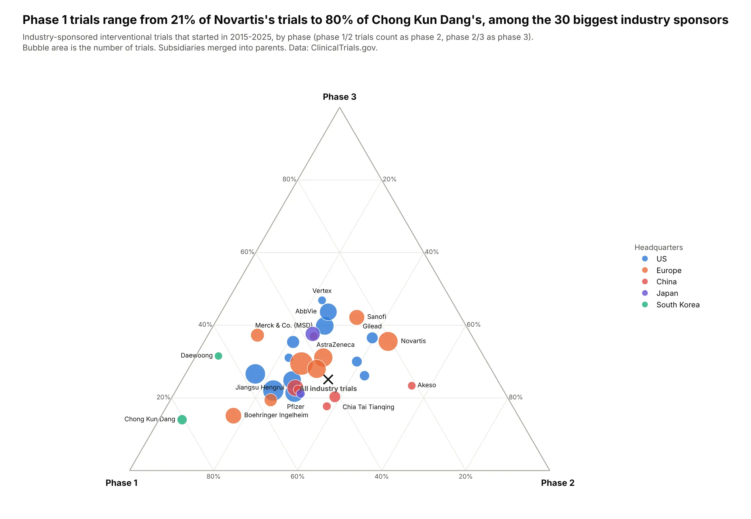
Among the 30 biggest industry sponsors of trials started in 2015-2025, the share in phase 1 ranges from 21% for Novartis to 80% for South Korea's Chong Kun Dang. Across all 41,391 industry trials, 40% were phase 1. Data: ClinicalTrials.gov, 2015-2025.

Tip: a cross for the all-industry average gives every sponsor a reference point, and only the extremes need labels.

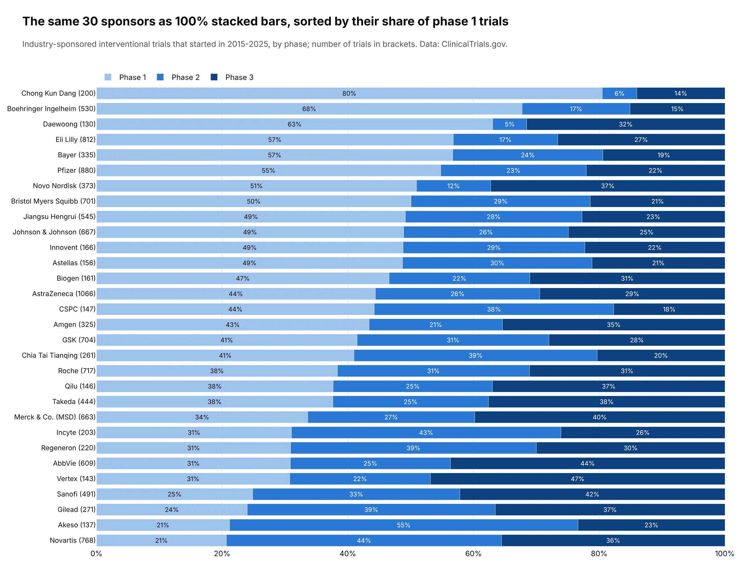
Another way to see it: 100% stacked bars sorted by phase 1 share give each sponsor's exact split, such as AstraZeneca's 44% phase 1, 26% phase 2 and 29% phase 3, but the clusters by region are harder to spot.

10. Paid work, unpaid work and leisure

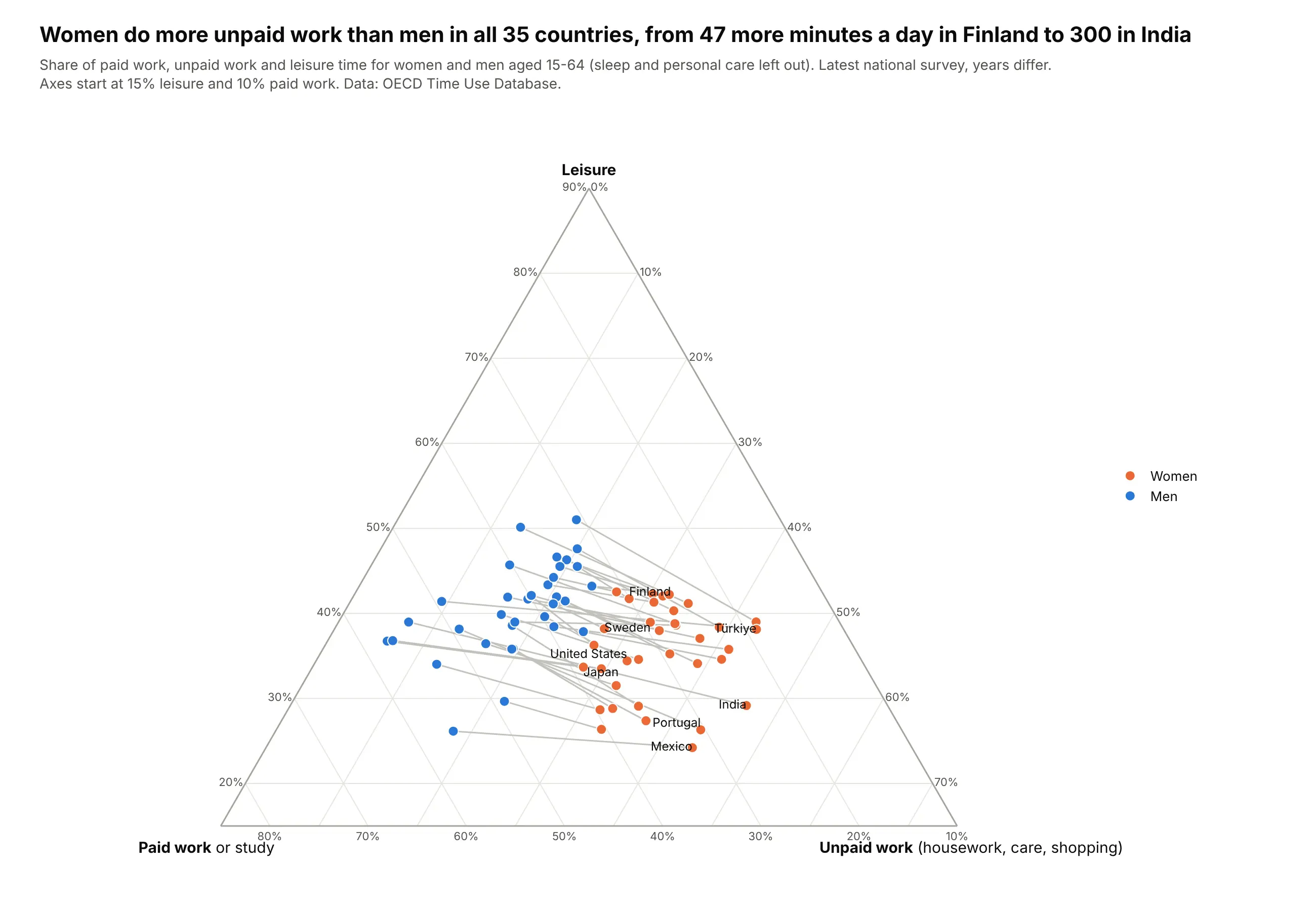
Women do more unpaid work than men in all 35 countries, from 47 more minutes a day in Finland to 300 in India. Every pair of points runs the same way, with women toward unpaid work and men toward paid work and leisure. Data: OECD Time Use Database.

Tip: a gray line between two Scatterternary points per country makes a dumbbell inside the triangle, drawn before the markers so they sit on top.

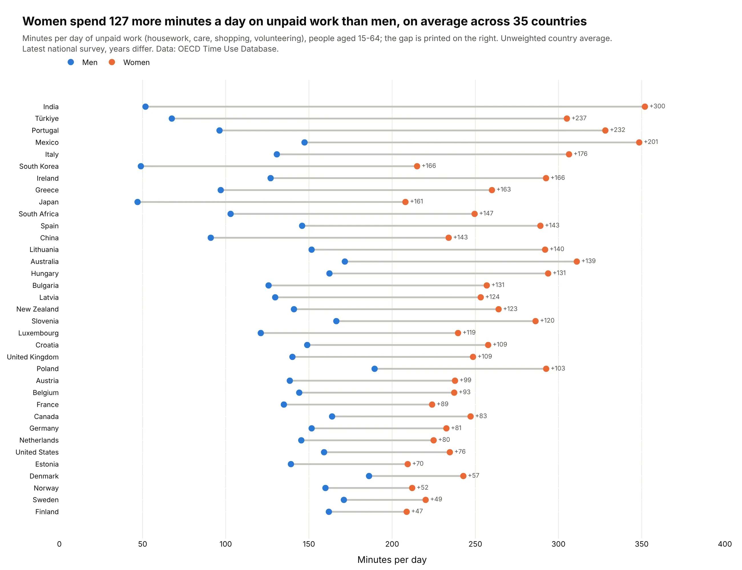
Another way to see it: a dumbbell chart of unpaid minutes alone ranks the countries exactly and shows the average gap of 127 minutes a day, but it leaves out the paid work and leisure that the ternary plot shows move the other way. See our dumbbell chart guide.

11. A three-way election

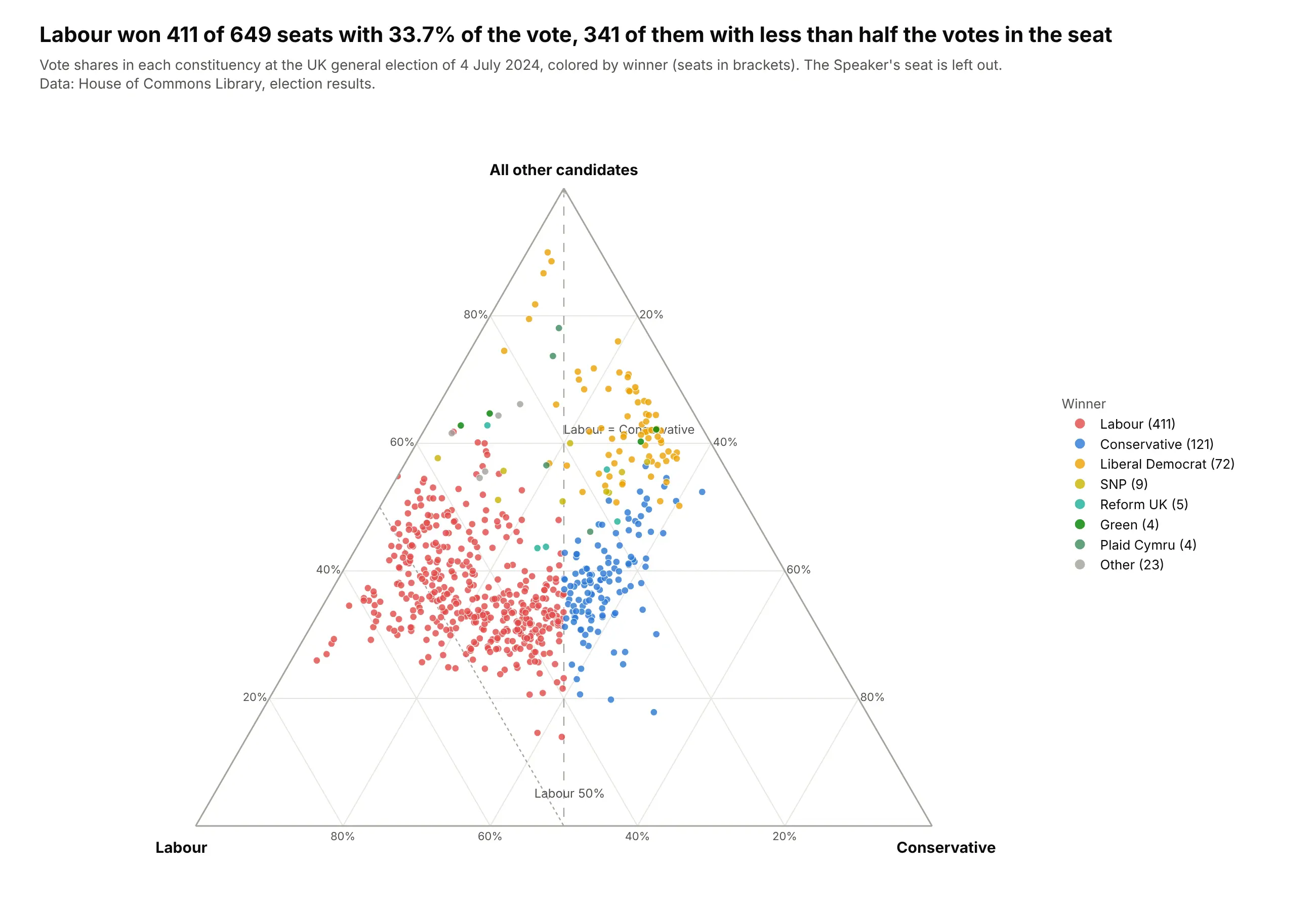
Labour won 411 of 649 seats in the 2024 UK general election with 33.7% of the vote, and 341 of those seats were won with less than half the votes because the rest of the vote was split between the Conservatives and everyone else. Each seat is a point, colored by its winner. Data: House of Commons Library, election results, 4 July 2024.

Tip: draw the reference lines (here Labour equal to Conservative, and Labour at 50%) as two-point Scatterternary lines before the markers, so readers can see which side of each line a seat falls on.