Line Charts - A Complete Guide

TL;DR

• A line chart plots values in order, usually over time, and joins them with a line, so the slope shows how fast something changed and the shape shows its trend, its cycles and its turning points.
• Line charts are also known as line graphs, line plots, curve charts, run charts and time series plots, and are similar to slope charts, bump charts, streamgraphs and small multiples.
• You can make a line chart with Plotly in one line of code with px.line in Python, or with a scatter trace in plotly.js, and the same chart can be animated with animation_frame or updated in real time in a Dash app.
• Use a log axis when values change by orders of magnitude, a step line for values that hold until the next change, and direct labels instead of a legend when you have a few lines.
• See 12 ways to draw a line chart below, all from the same 40 years of daily oil, gas and gasoline prices: raw, smoothed, log, indexed, small multiples, seasonal overlay, bands, events, filled gaps, two axes, sparklines and year-over-year change.

What is a line chart?

Line charts look like this:

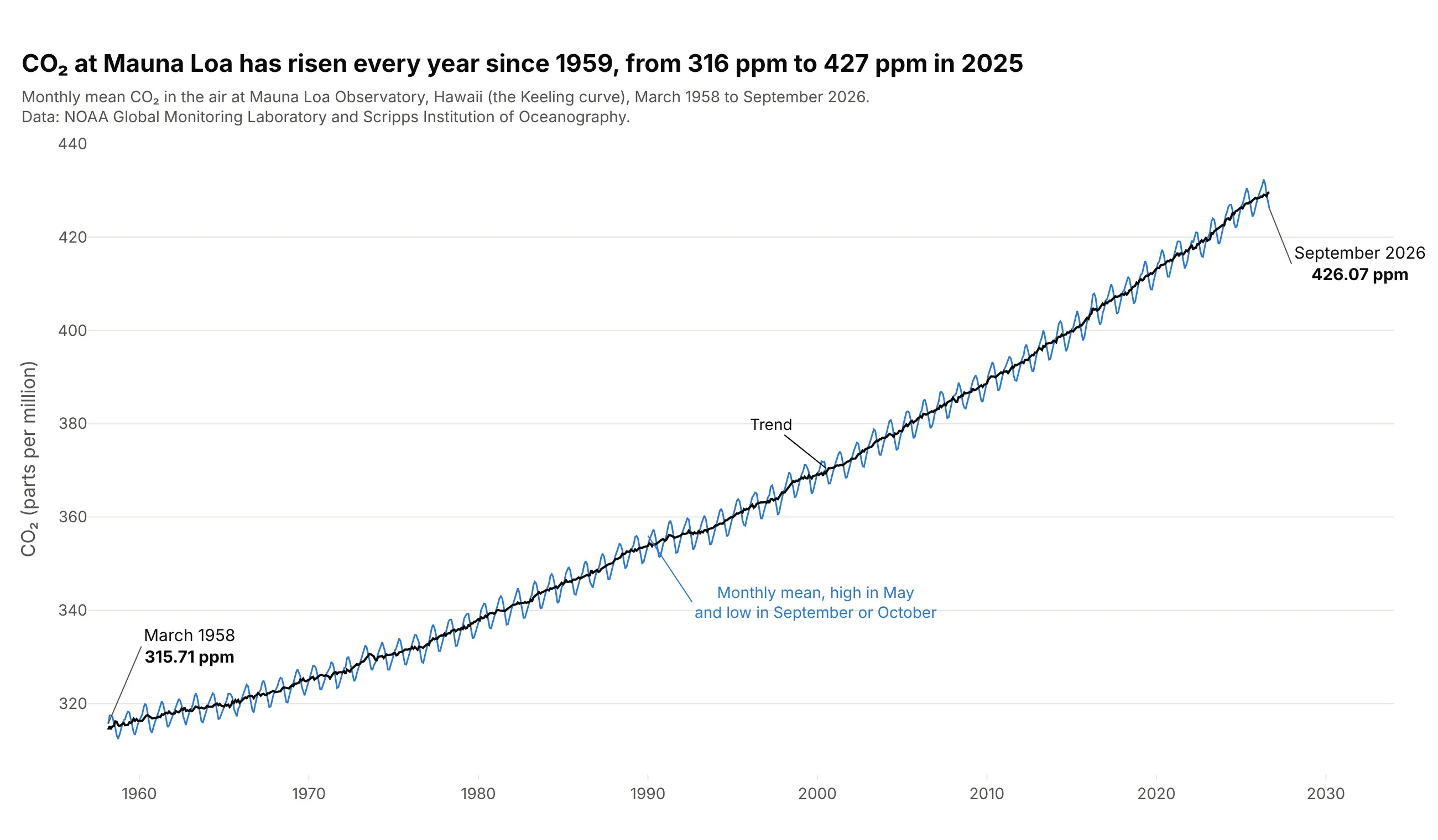
Data: NOAA Global Monitoring Laboratory and Scripps Institution of Oceanography, monthly mean CO₂ at Mauna Loa.

How do you read a line chart? In the example above, notice these things:

• Each point is one month's average CO₂ at Mauna Loa, placed at its date and its value, and the line joins the 823 months in order, from 315.71 ppm in March 1958 to 426.07 ppm in September 2026.
• The steepness of the line is the rate of change. The dark trend line rose 0.86 ppm a year on average in the 1960s and 2.63 ppm a year from 2016 to 2025, which is why the curve bends upward.
• The sawtooth is the yearly cycle: the highest month was May in 61 of the 67 full years from 1959 to 2025, and the lowest was September or October in all of them, a swing of about 6 ppm.
• The y axis starts at 305 ppm, not zero. A line chart is read by its slope and position rather than by the length of a bar, so a zoomed axis is fine as long as it's labeled.

It's often used for charts like these:

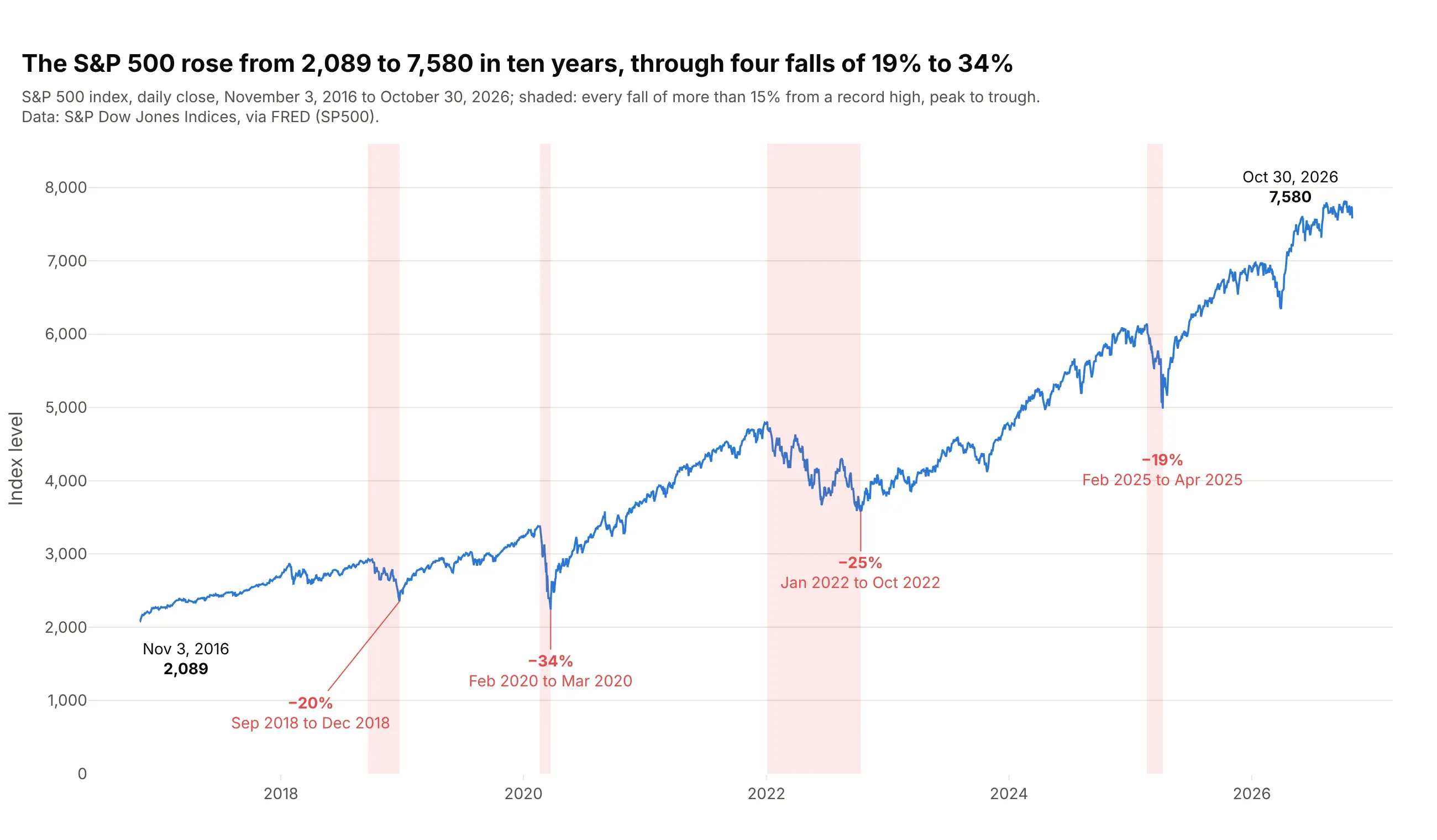
Stock prices. The S&P 500 closed at 2,089 on November 3, 2016 and 7,580 on October 30, 2026, and the shaded bands mark the four times it fell more than 15% from a record high, by 19% to 34%. Data: S&P Dow Jones Indices via FRED (SP500).

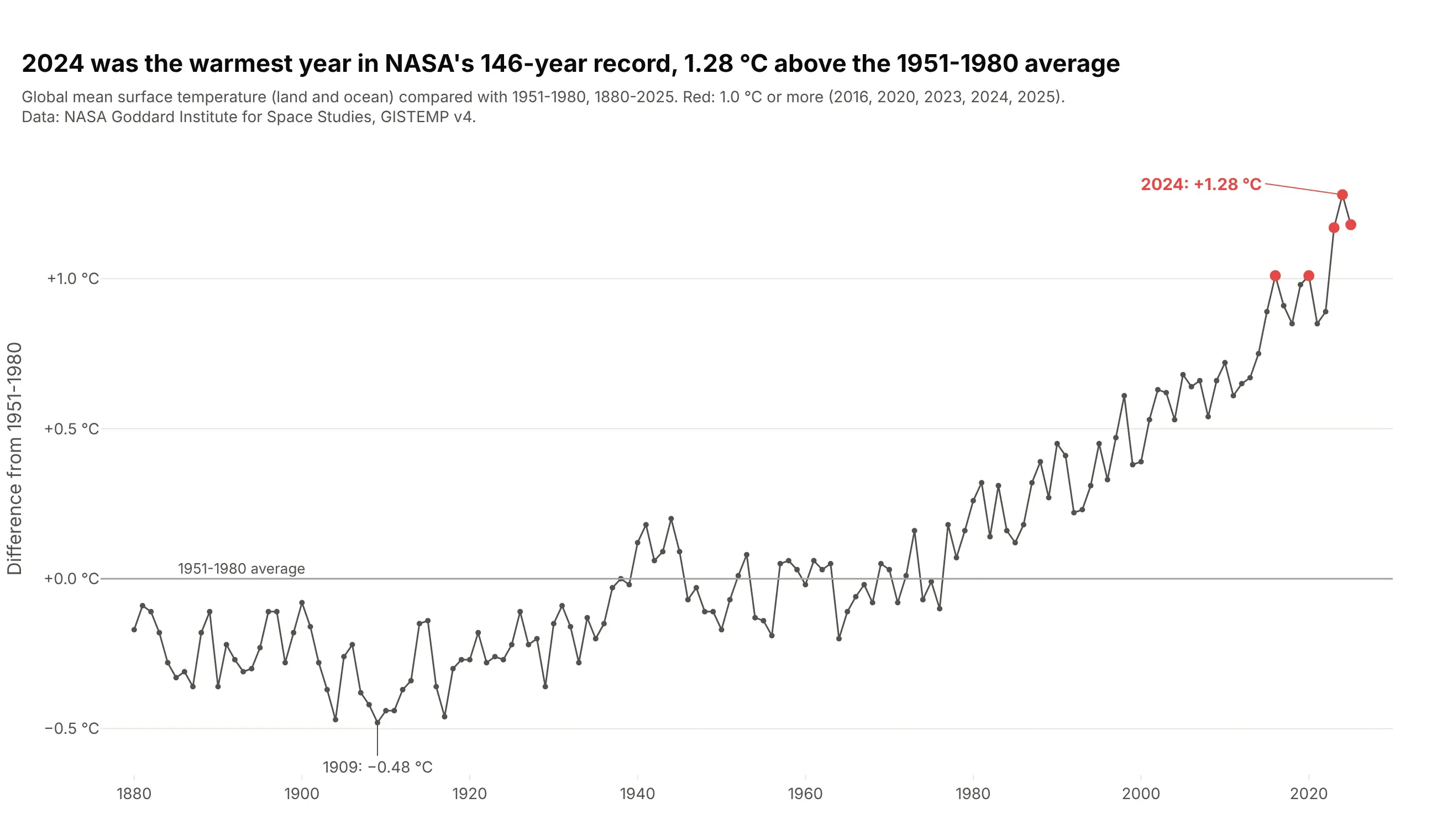
Temperature records. 2024 was the warmest year in NASA's 146-year record at 1.28 °C above the 1951-1980 average, and all five years at 1.0 °C or more came after 2015. Data: NASA GISS, GISTEMP v4.

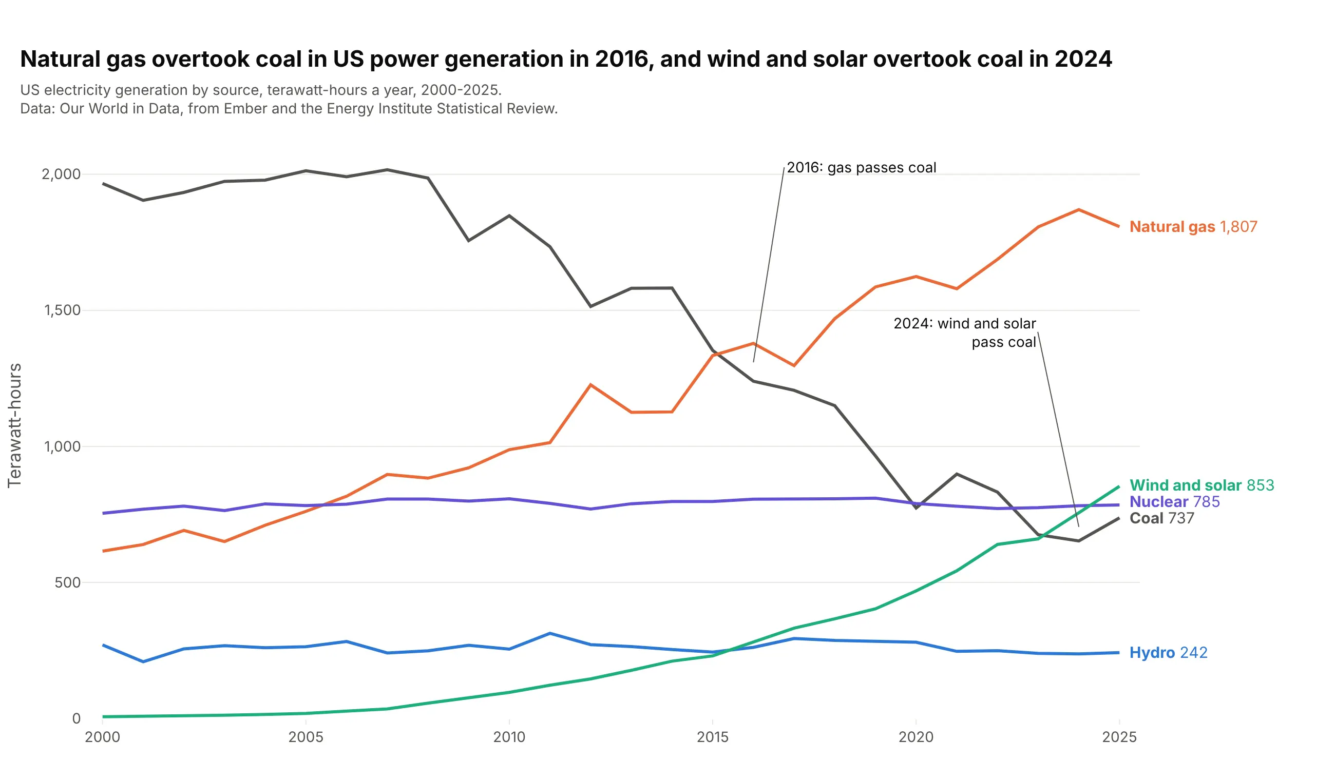
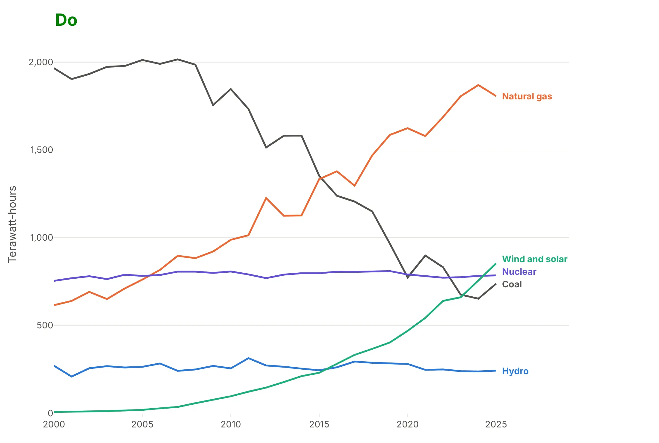
Several series that cross. Natural gas passed coal in US power generation in 2016, and wind and solar passed coal in 2024, at 756 against 652 TWh. Data: Our World in Data, from Ember and the Energy Institute.

A short history

Wikipedia's line chart article credits early line charts to Francis Hauksbee, Nicolaus Samuel Cruquius, Johann Heinrich Lambert and William Playfair, and says that in 1786 Playfair "plotted ten years of money spent by the Royal Navy". His Commercial and Political Atlas of that year contained 43 time-series plots and one bar chart, many of them England's imports and exports drawn as lines over the years. The data behind the 1786 charts isn't published in a form we could redraw, so here is a later Playfair chart from 1821, redrawn with Plotly from his own values, with wheat prices as bars and a mechanic's weekly wage as a line:

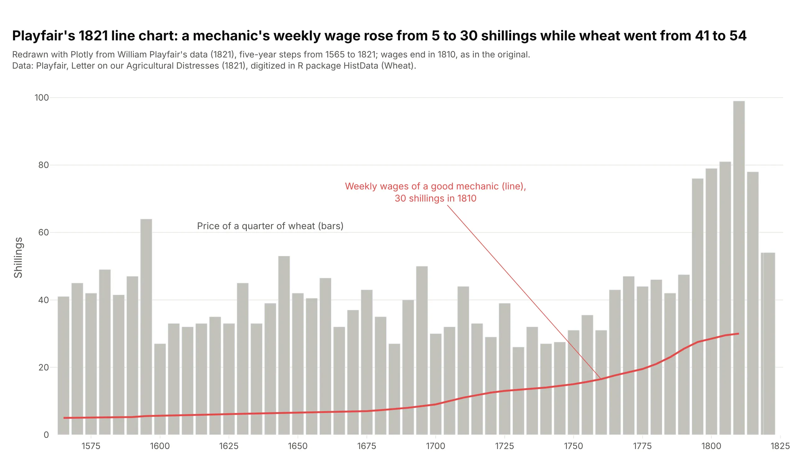
Data: Playfair (1821), Letter on our Agricultural Distresses, digitized in R's HistData package; see Friendly and Denis (2005) for the history. A well-known modern line chart is the one at the top of this page: Charles David Keeling's CO₂ record at Mauna Loa, which started in 1958 (Keeling 1960).

Alternatives to a line chart

Here's the same US electricity data drawn six ways, starting with the line chart, where every trend and both crossings are visible. The others are better for some questions, worse for some, or just different:

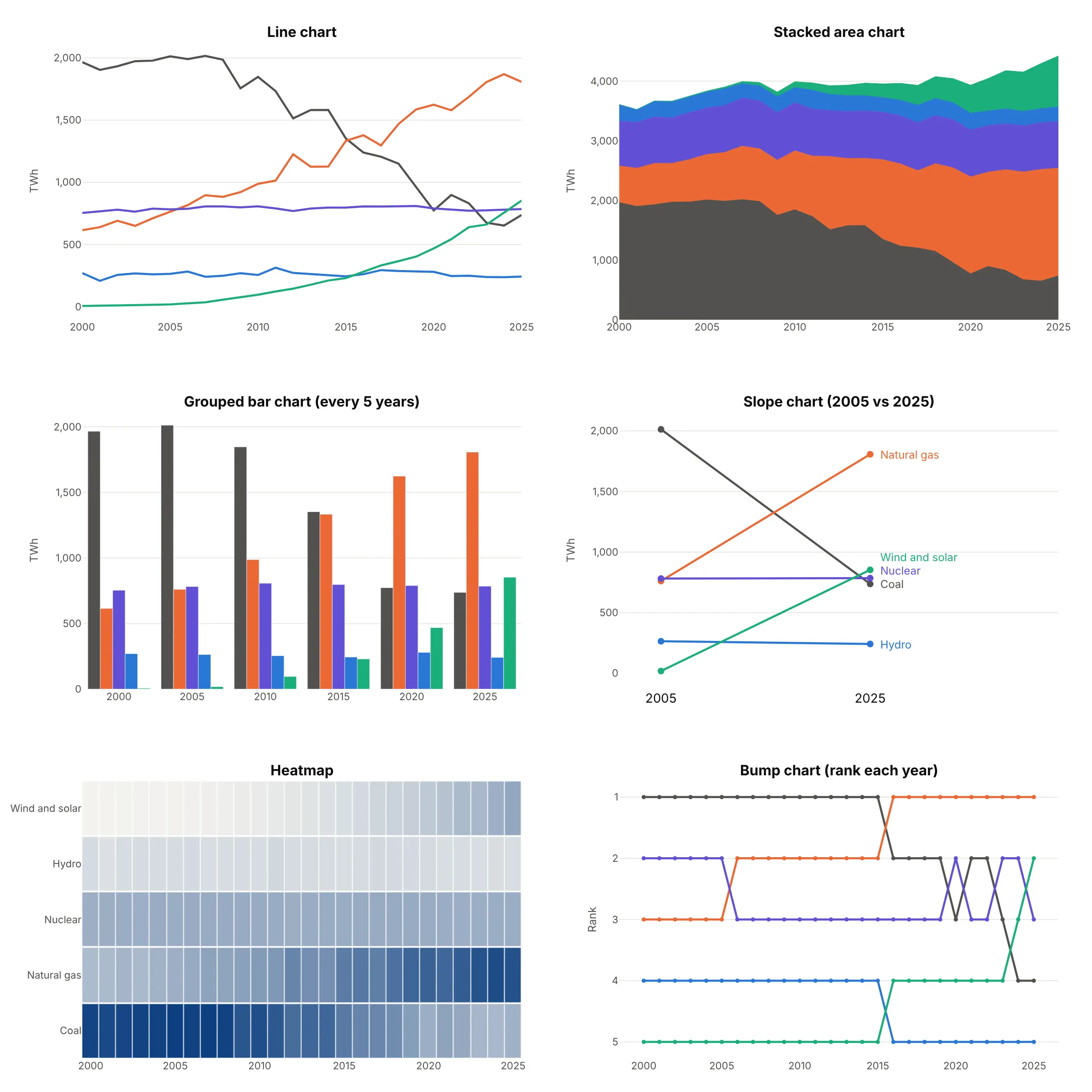
• Stacked area chart (better for the total). It shows that total generation grew from about 3,600 to 4,400 TWh, but only the bottom layer (coal) can be read against a flat baseline, so the crossings disappear. The streamgraph guide covers the centered version.
• Grouped bar chart (works too, for a few dates). Bars every five years compare sources within a year well, but the years in between are gone and the crossing in 2016 falls between two groups.
• Slope chart (better for two dates). 2005 against 2025 shows who gained and who lost in one glance, but hides the path, such as coal's flat years before 2008.
• Heatmap (worse here). Color is harder to compare than position, so the crossing years are hard to find, though a heatmap scales to hundreds of series.
• Bump chart (different). It plots rank instead of value, which makes every crossing obvious but hides how far apart the sources are.

Animated and real-time line charts

"Animated line chart" can mean two things, and Plotly does both.

Animate a line chart with px.line and animation_frame

px.line takes an animation_frame column and draws one frame per value, with a play button and a slider. Each frame shows only the rows for that value, so it fits data where every frame is a whole line, like the Treasury yield curve at each month-end:

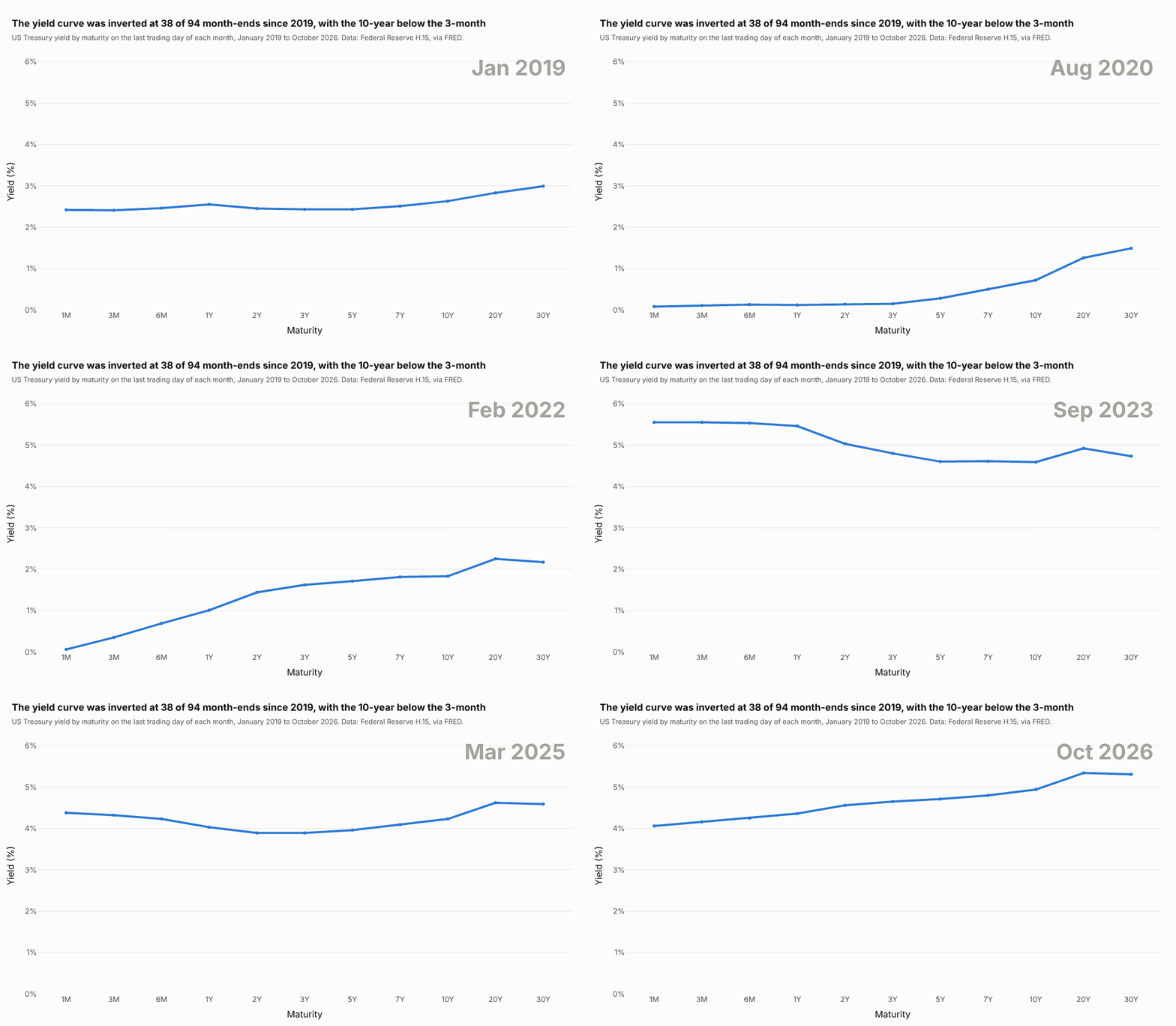
Data: Federal Reserve H.15 via FRED (DGS1MO to DGS30).

Set range_y (and range_x if needed), because the axes don't rescale between frames. To animate a line that draws itself over time, repeat the data so each frame holds every point up to that date:

The Plotly animations documentation covers frame duration, easing and buttons.

Make a real-time line chart that scrolls

A real-time line chart adds new points as they arrive and drops the oldest ones, so the window scrolls. This is one hour of Great Britain's electricity grid frequency at one reading per second, the kind of signal grid operators watch live:

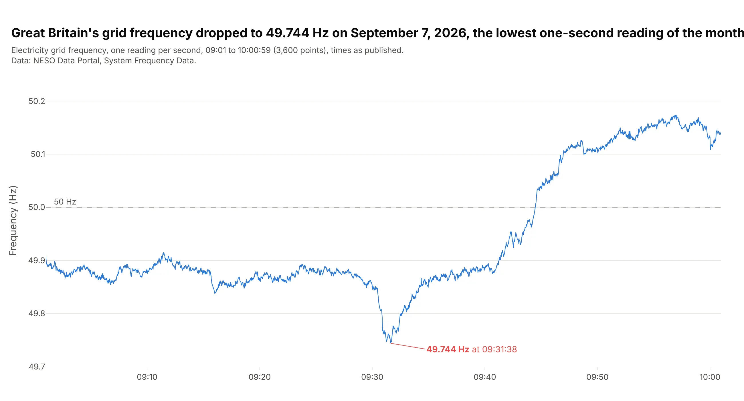
Data: NESO Data Portal, System Frequency Data.

A regular Dash callback sends its outputs once, when the function returns, so a live chart used to need a dcc.Interval timer that asked the server for new points every few hundred milliseconds. Dash 4.5 added streaming callbacks, which are async def functions that use yield instead of return, and each yielded value reaches the browser as soon as it's produced, so the page doesn't have to keep asking. Yielding a Patch sends only the change instead of the whole figure, which here is five new readings plus deleting the five oldest once 600 are on screen, because a Patch can't cap how many points a list keeps.

This needs Dash 4.5 or later (pip install "dash[async,shared_storage]>=4.5"), and LocalSharedStorage is the shared storage that streaming over HTTP requires when the app runs on one machine:

This replays the recorded hour at 20 times real speed, and here it is running:

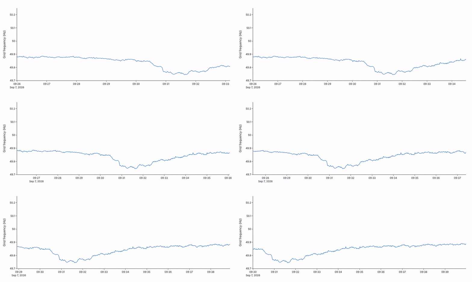
In your own app, replace the asyncio.sleep and chunk = ... lines with an awaited read from your sensor, message queue or database, because a blocking call such as time.sleep would hold up the stream. In plain JavaScript, Plotly.extendTraces does the same job, and plotly.js is free and open source under the MIT license:

The plotly.js streaming documentation has more patterns.

How to make a line chart

With AI

ChatGPT, Claude Code, GitHub Copilot, Cursor and other AI tools are excellent at writing Plotly code. Name Plotly in the prompt, and say what the x axis is, how many lines you want and how they should be labeled:

With Plotly Studio

Plotly Studio is a desktop app where you point an AI at a dataset and it builds charts and a Dash app around your questions. Ask for a line chart the same way:

Show a line chart of monthly CO₂ at Mauna Loa since 1958, the monthly means as a thin line and the deseasonalized trend as a thicker dark line, with the first and latest months labeled.

Make a line chart in Python or JavaScript

This is the code AI tools write under the hood. In Python, px.line makes a line chart in one line of code, and the Plotly line chart documentation covers markers, colors and facets:

px.line takes a column for y, or a list of columns as here, and a color column for data in long format (one row per date and series). It returns a figure with one go.Scatter trace per line, with mode="lines", which you can style with fig.update_traces.

In JavaScript, a plotly.js line chart is a scatter trace with mode: "lines" (or "lines+markers"). This is a simple, complete example you can save as an HTML file:

The plotly.js line chart documentation has more JavaScript line chart examples, and the log plot page covers logarithmic axes.

Share it

Every Plotly chart has a Share chart button (the cloud icon in its toolbar) that uploads it to Plotly Cloud and gives you a link. Only you can see it until you change its visibility.

For a live app, put the chart in a Dash app and publish it with the Plotly Cloud CLI. Coding agents can run these commands for you:

If your data has to stay in your own cloud or data center, publish to Dash Enterprise instead.

Dos and don'ts

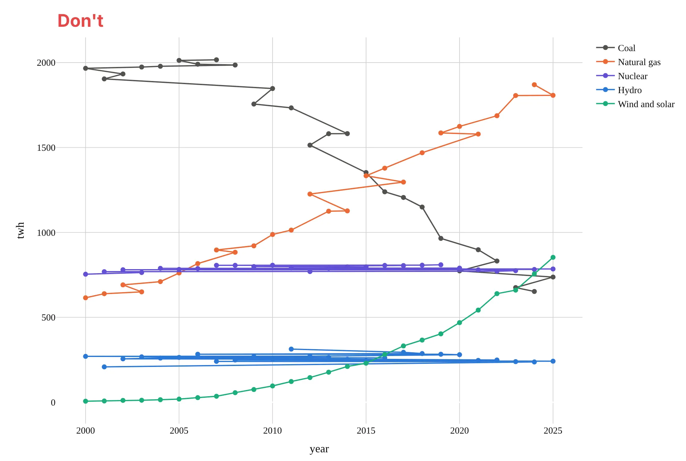
Most of the work in a published line chart is getting the data in order, keeping the lines clean and labeling them where readers look. Here is the US electricity data both ways, in the same colors.

Don't plot rows that aren't sorted by date (here they're sorted by value, as after a sort_values), which makes each line zigzag back and forth in time, put markers on every point, rely on a legend far from the lines, or use a default serif font and raw column names as axis titles:

Do sort by date, draw lines without markers when there are many points, label each line at its end and give the axis a unit:

Choose the line shape

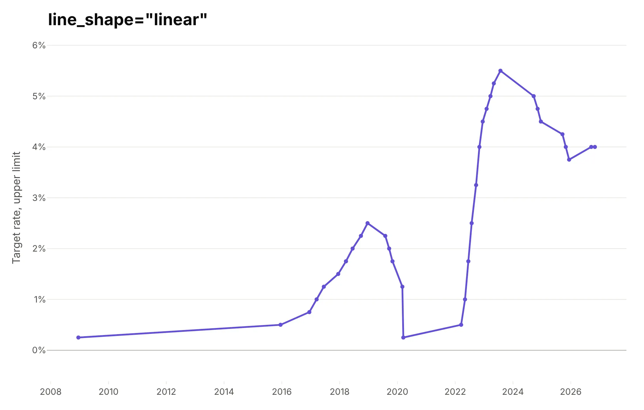
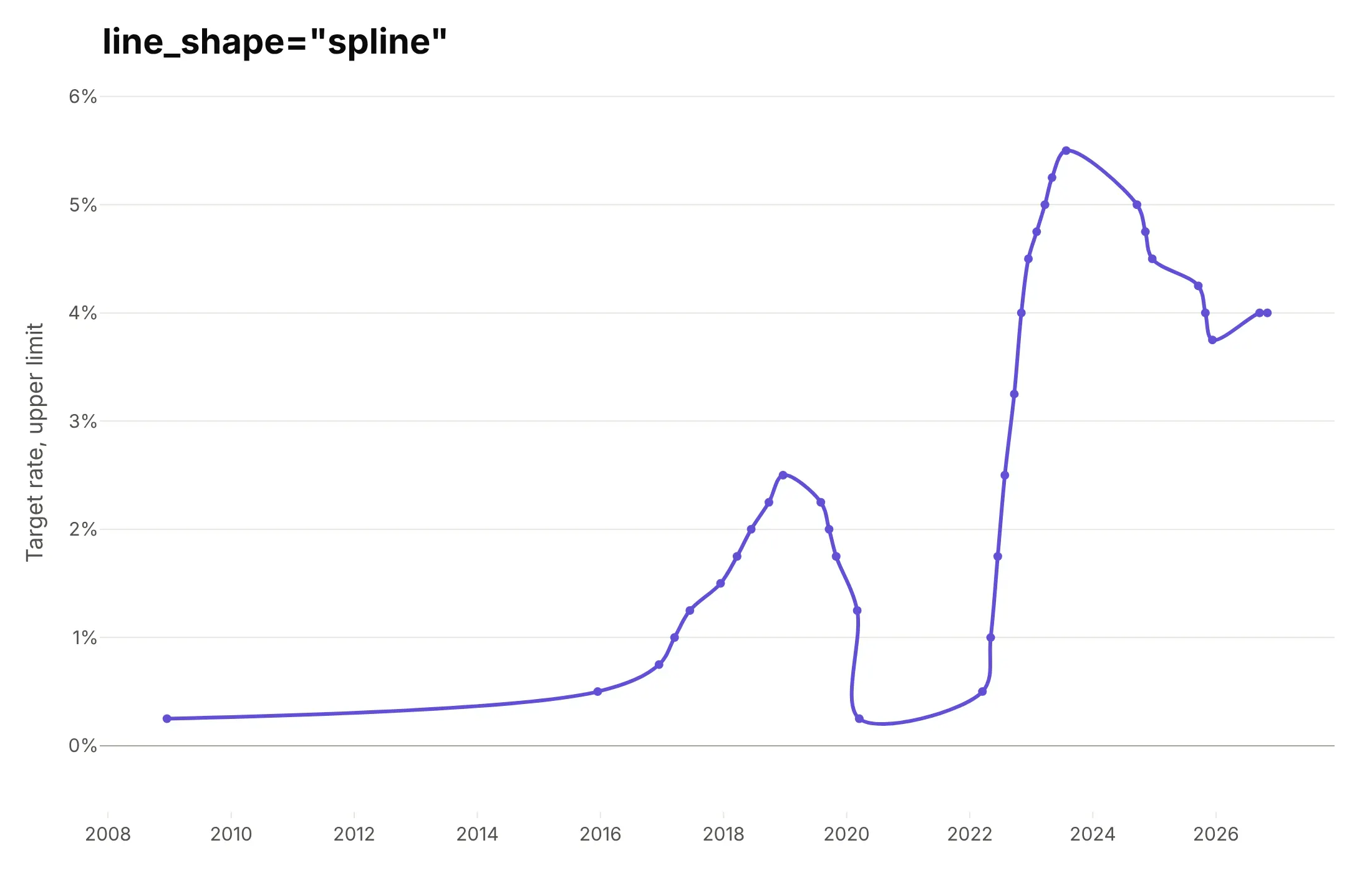
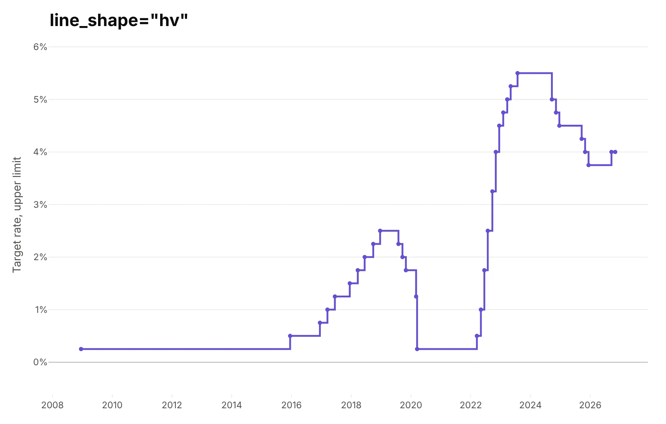
The line_shape option (line.shape in JavaScript) changes how Plotly joins the points, and on data that changes in steps, like the Federal Reserve's target rate, it changes what the chart claims.

linear. The default draws a straight line between decisions, which shows gradual moves that never happened, such as a slow rise from 0.25% in 2008 to 0.50% in 2015.

spline. A smoothed curve (the "spline line chart" in JavaScript libraries) looks soft, but here it bends backward in time in March 2020 and dips below the 0.25% floor, so use it only for smooth measurements with no sharp changes.

hv. A step line holds each value until the next point, which is exactly how a policy rate works.

Checklist

Do

• Sort the data by the x value before you plot it.
• Label each line at its end when there are up to about six, and use a legend only when there are more.
• Use a log axis when values span orders of magnitude, and say so in the subtitle.
• Use a step line (line_shape="hv") for values that hold until they change, like rates and prices set by decision.
• Shade periods that explain the line (recessions, outages, trials) with add_vrect behind it.
• Write a title that states the takeaway.

Don't

• Draw more than about six lines in one chart; use small multiples or highlight one line and gray the rest.
• Use a spline on data with sharp changes.
• Join points across a gap in the data; leave the None values in and Plotly breaks the line (connectgaps=False, the default).
• Put two unrelated series on two y axes, since the crossing point then depends on how you scaled each axis.

Options to customize

A line chart in Plotly is px.line or a go.Scatter trace with mode="lines", so these are the options that matter most. The full lists are in the px.line reference and the scatter trace reference.

1. px.line(x=..., y=...): the x column (usually a date) and one or more y columns.
2. color, line_dash, line_group: one line per group, told apart by color or dash pattern, or by group alone.
3. markers=True or mode="lines+markers": a dot at each point, for charts with tens of points.
4. line_shape (line.shape): "linear", "spline", "hv", "vh", "hvh" or "vhv".
5. line.width, line.dash, line.color: thickness, dashes and color of each line.
6. connectgaps: whether to bridge missing values; the default leaves a gap.
7. yaxis.type="log": a logarithmic axis; in plotly.js, layout.yaxis.type: "log".
8. hovermode="x unified": one hover box with every line's value at that date.
9. add_vrect, add_hline, add_annotation: shaded periods, reference lines and labels at the end of each line.
10. facet_col, facet_row: small multiples, one panel per group.
11. animation_frame: one frame per value, with a play button and slider.
12. px.line_3d: lines in three dimensions, with a z column.
13. go.Scattergl: WebGL rendering for very large or many traces.

12 ways to draw a line chart

The same data can make very different line charts, depending on what you smooth, rescale, highlight or split apart. We took 40 years of daily US energy spot prices from the EIA (WTI and Brent crude oil, Henry Hub natural gas and New York Harbor gasoline, 33,532 prices in all) and drew them 12 ways.

1. The raw daily line

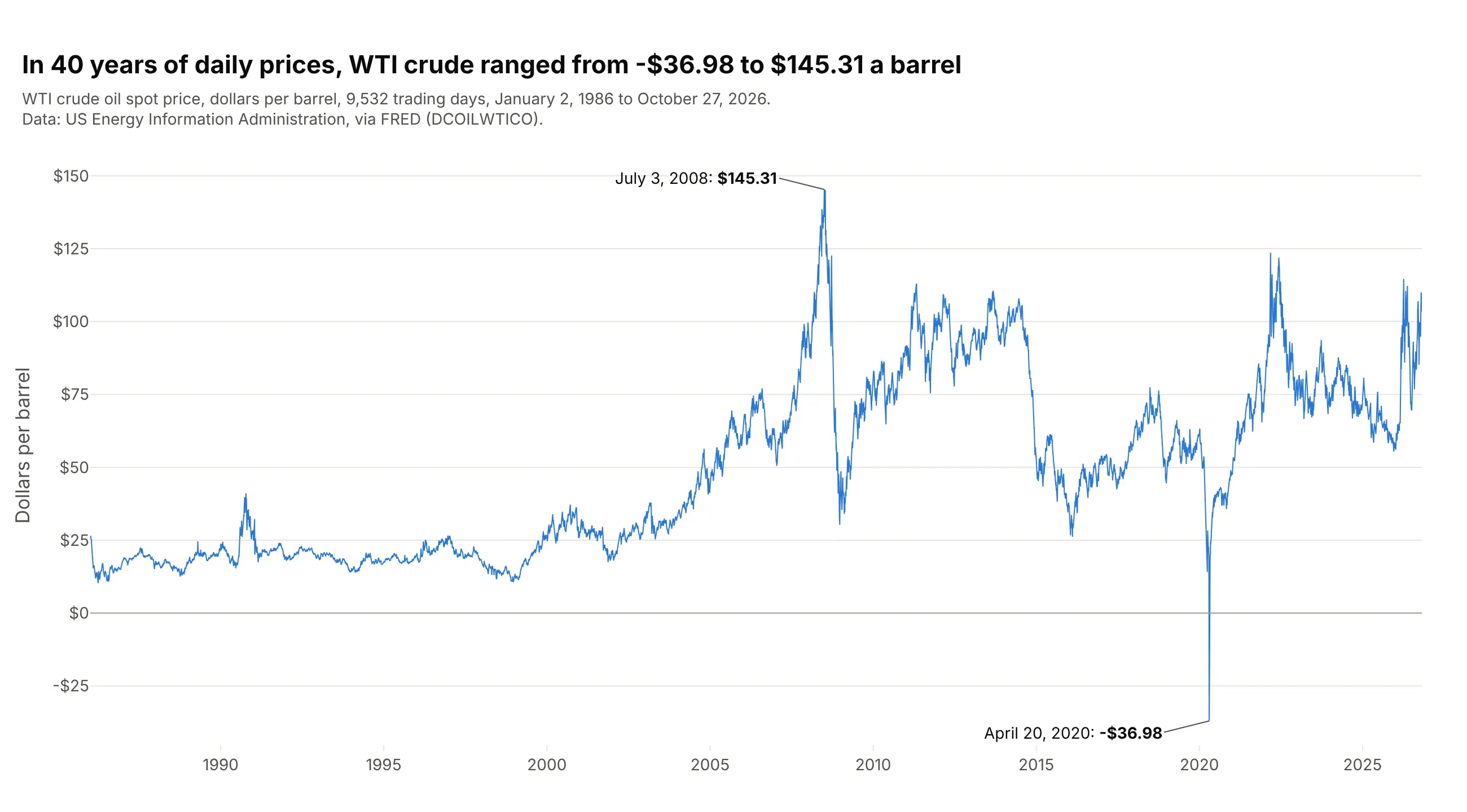
Every trading day as one point, joined in order, is the honest starting point: nothing is averaged away, so the July 2008 peak and the one negative day in April 2020 are both there. With 9,532 points the line is dense, so short-term moves blur into a texture and it's hard to read any single month. In Plotly this is px.line(df, x="date", y="price") with a thin line (line_width=1).

Prompt: Get daily WTI crude oil spot prices from FRED (series DCOILWTICO, from the US EIA, since 1986) into a table with date and price. Make a plotly line chart with px.line, a 1 px blue line, a gray line at $0, dollar tick labels written as -$40 rather than $-40, and labels on the highest and lowest days with their dates and prices.

2. A rolling average over the raw line

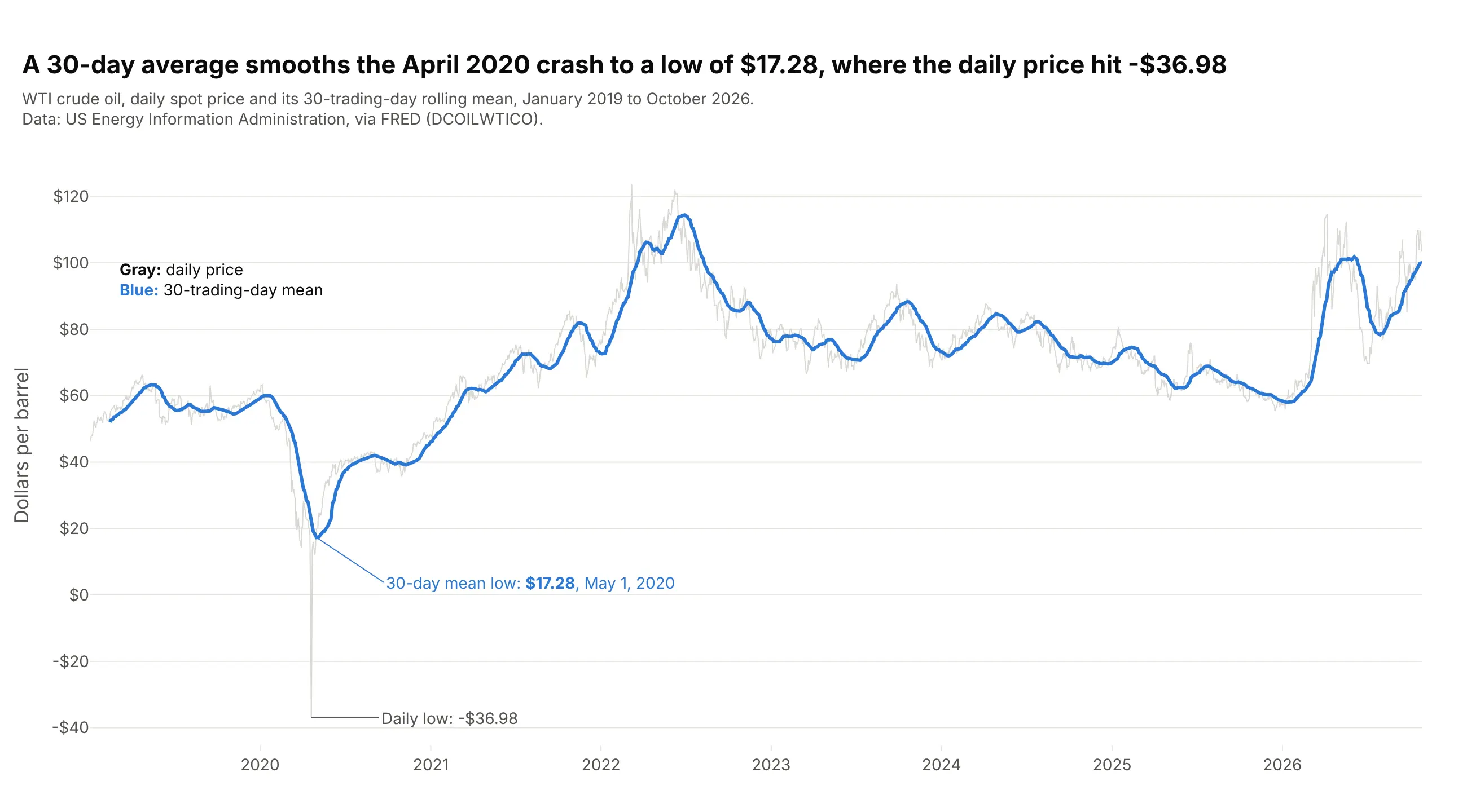
A 30-trading-day rolling mean drawn over the raw price in light gray shows the trend and keeps the noise as context. The mean's low was $17.28 on May 1, 2020, so it hides the negative day entirely, which is the trade-off of any smoothing. Compute it with df.price.rolling(30).mean() and add it as a second trace, raw first so the mean sits on top.

Prompt: Get daily WTI crude oil spot prices from FRED (DCOILWTICO, US EIA) since January 2019. Make a plotly line chart with the daily price as a 1 px light gray line and its 30-trading-day rolling mean (pandas rolling(30).mean()) as a 3 px blue line on top. Label the rolling mean's lowest point and the daily low, and explain the two lines in a small legend note on the chart.

3. A log axis

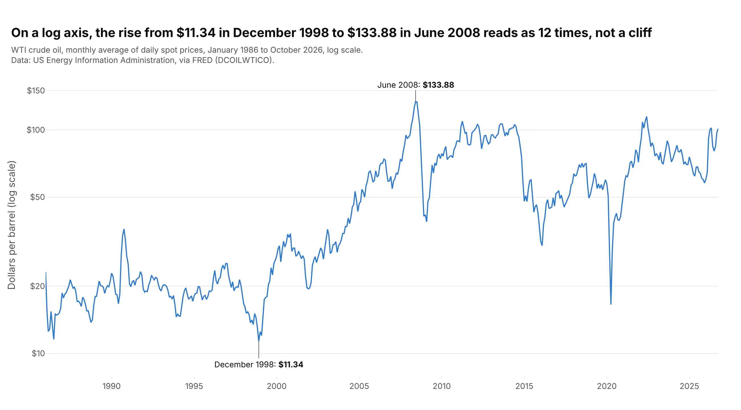
On a log axis equal heights are equal percentage changes, so the rise from $11.34 a barrel in December 1998 to $133.88 in June 2008, about 12 times, looks as large as it was, and the cheap years before 2000 are readable instead of squeezed against the bottom. Use it when values span an order of magnitude or more and you care about growth rates. In Plotly, log_y=True (or yaxis.type="log"); a log axis can't show zero or negative values, which is why this chart uses monthly averages.

Prompt: Get daily WTI crude oil spot prices from FRED (DCOILWTICO, US EIA) since 1986 and resample them to monthly averages. Make a plotly line chart with log_y=True, ticks at $10, $20, $50, $100 and $150, and the lowest and highest monthly averages labeled with their month and price. Say "log scale" in the subtitle.

4. Indexed to 100

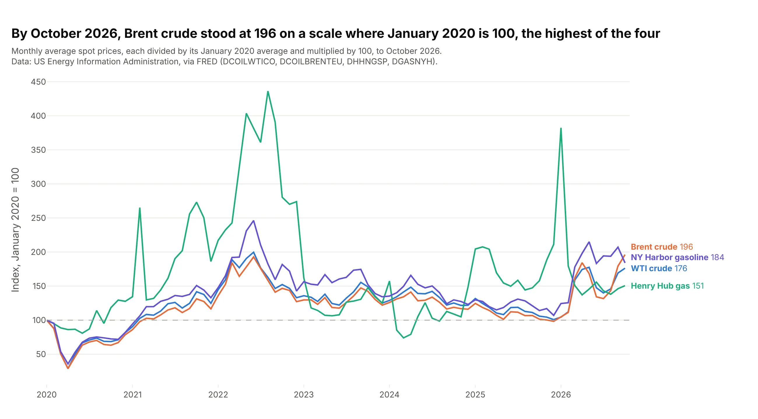
Dividing every series by its own starting value puts dollars per barrel, per million Btu and per gallon on one scale, so the chart compares percentage change instead of price. By October 2026 Brent crude stood at 196, nearly double its January 2020 average, and the Henry Hub line shows how much more volatile gas is than oil. Compute df / df.iloc[0] * 100 before plotting and add a dashed add_hline(y=100).

Prompt: Get daily spot prices from FRED for WTI (DCOILWTICO), Brent (DCOILBRENTEU), Henry Hub gas (DHHNGSP) and New York Harbor gasoline (DGASNYH), all from the US EIA, since January 2020. Resample to monthly averages and divide each series by its January 2020 value times 100. Make a plotly line chart with one colored line per series, a dashed line at 100, and each line labeled at its right end with its latest index value.

5. Small multiples

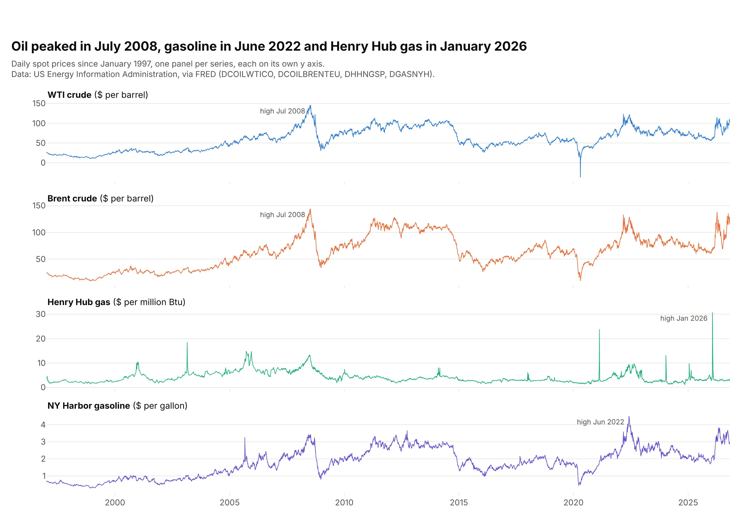
When series have different units, one panel each with its own y axis is clearer than one crowded chart. The shared x axis still lines up the events: both crudes peaked in July 2008, gasoline in June 2022 and Henry Hub gas in January 2026. In Plotly Express this is facet_row="series" with fig.update_yaxes(matches=None), or make_subplots(rows=4, shared_xaxes=True).

Prompt: Get daily spot prices from FRED for WTI (DCOILWTICO), Brent (DCOILBRENTEU), Henry Hub gas (DHHNGSP) and New York Harbor gasoline (DGASNYH) since 1997 into a long table (date, series, price). Make a plotly line chart with facet_row="series", independent y axes (matches=None), a shared x axis, one color per series, each panel titled with its unit, and each series' highest day marked with its month.

6. Year-over-year overlay with one year highlighted

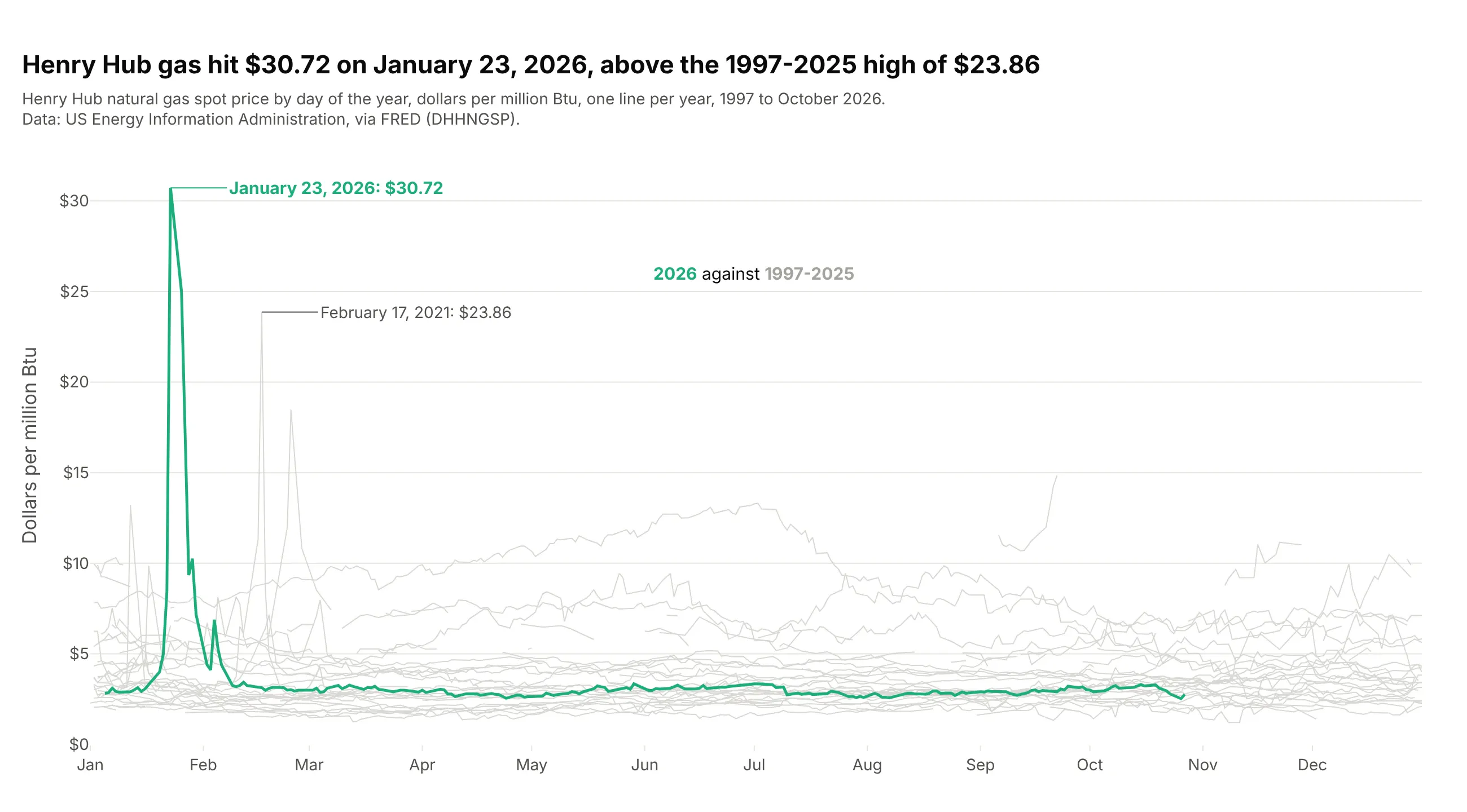
Putting the day of the year on the x axis and drawing one line per year shows the seasonal pattern, and coloring a single year against the gray history answers "is this year unusual?". Henry Hub gas reached $30.72 on January 23, 2026, above the 1997-2025 high of $23.86 in February 2021, and then stayed between $2.52 and $3.34 from March to October. Build it by mapping each date to the same year ("2000-" + date.strftime("%m-%d")) and drawing the highlighted year last so it sits on top.

Prompt: Get daily Henry Hub natural gas spot prices from FRED (DHHNGSP, US EIA) since 1997. Make a plotly line chart with day of the year on the x axis (map every date to the year 2000), one 1 px light gray line per year from 1997 to 2025, and 2026 as a 2.5 px green line drawn last. Break lines where data is missing for more than a week, and label the 2026 high and the previous record.

7. A min/max band

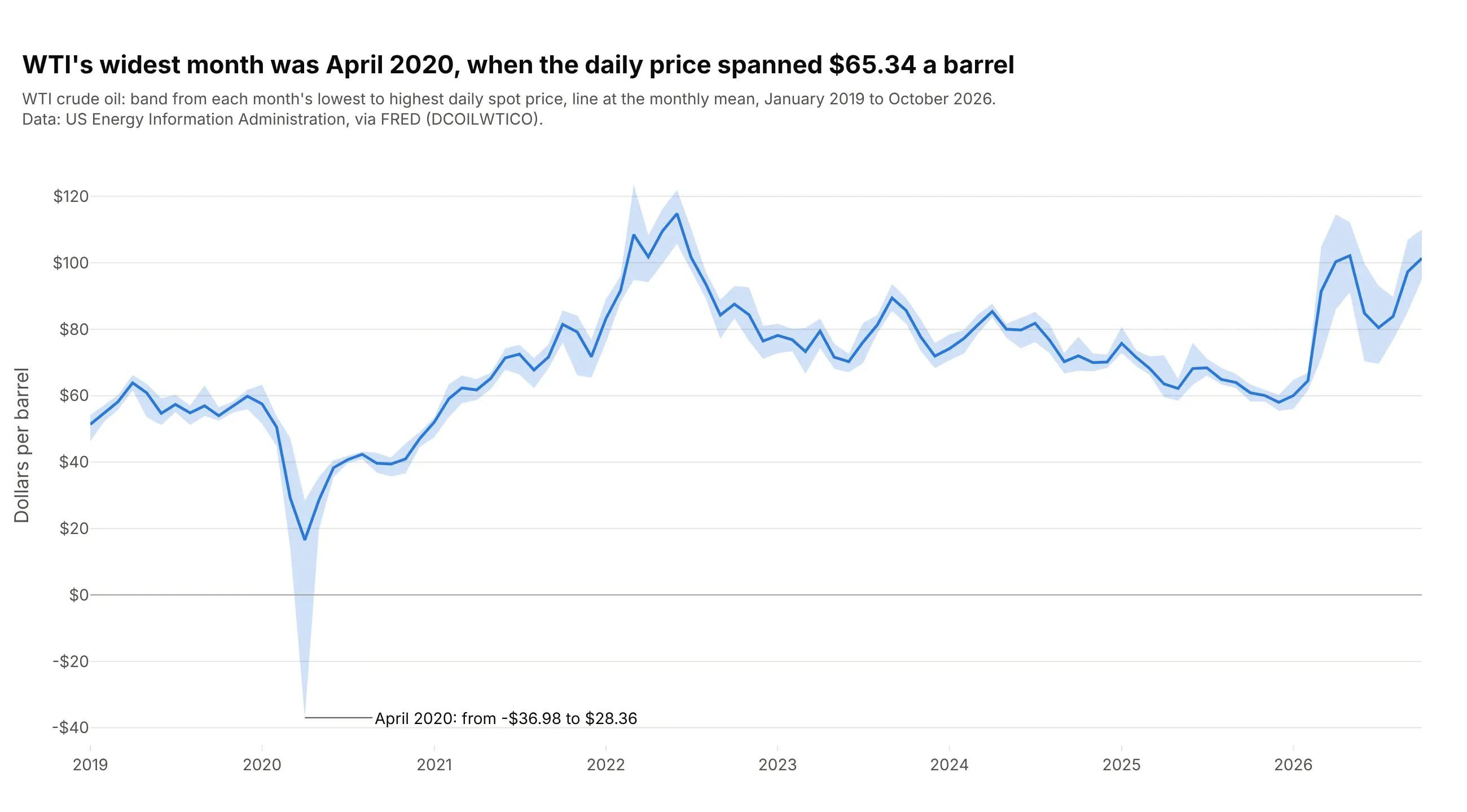
A shaded band from each month's lowest to highest daily price, with the monthly mean as a line, shows both the level and how much the price moved within the month. April 2020 stands out with a range of $65.34 a barrel, from -$36.98 to $28.36. The same pattern draws forecast intervals and confidence bands: add the upper bound, then the lower bound with fill="tonexty", then the line.

Prompt: Get daily WTI crude oil spot prices from FRED (DCOILWTICO, US EIA) since January 2019 and compute each month's minimum, maximum and mean. Make a plotly chart with the maximum as an invisible line, the minimum as an invisible line with fill="tonexty" in light blue, and the mean as a 2.5 px blue line on top. Label the month with the widest range.

8. Annotated events

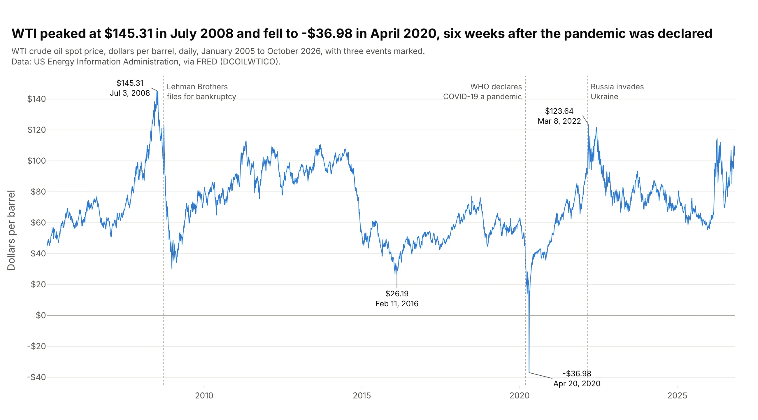
Labels for the turning points and a few dated events turn a price chart into a timeline the reader can follow without a separate explanation. WTI peaked at $145.31 on July 3, 2008 and fell to -$36.98 on April 20, 2020, six weeks after the WHO declared COVID-19 a pandemic on March 11. Use add_vline for the events and add_annotation for the values, and keep it to a handful, because every label competes with the line.

Prompt: Get daily WTI crude oil spot prices from FRED (DCOILWTICO, US EIA) since 2005. Make a plotly line chart with a dotted add_vline and a short gray label for three events (Lehman Brothers' bankruptcy on September 15, 2008, the WHO pandemic declaration on March 11, 2020 and Russia's invasion of Ukraine on February 24, 2022), and add_annotation labels with price and date on the 2008 high, the 2016 low, the April 2020 low and the 2022 high.

9. Two lines with the gap filled

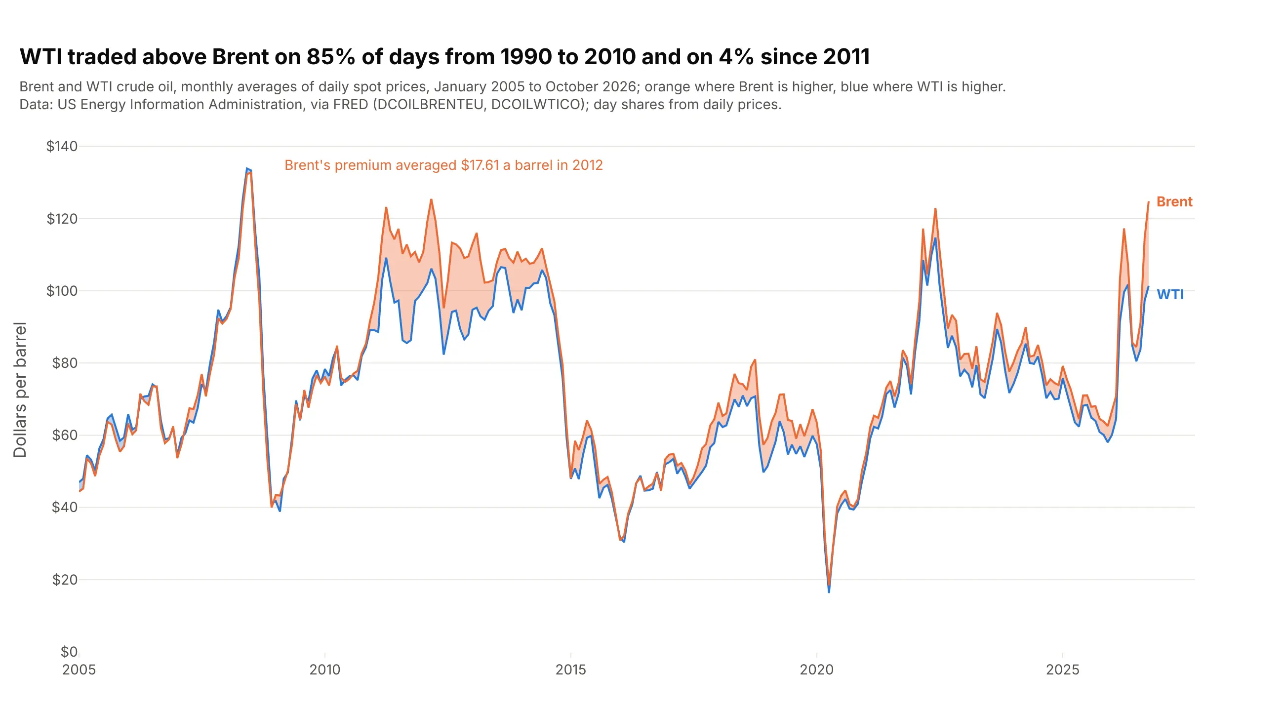
Shading the area between two lines turns attention from the levels to the difference. WTI traded above Brent on 85% of days from 1990 to 2010 and on 4% of days since 2011, and Brent's premium averaged $17.61 a barrel in 2012. In Plotly, draw the lower of the two as an invisible line and the higher as a line with fill="tonexty", once for each direction so each gets its own color.

Prompt: Get daily Brent (DCOILBRENTEU) and WTI (DCOILWTICO) spot prices from FRED (US EIA) since 2005 and resample to monthly averages. Make a plotly line chart with both lines, and fill the area between them with fill="tonexty" in orange where Brent is higher and in blue where WTI is higher. Put the share of days WTI traded above Brent, before and after 2011, in the title.

10. Two y axes (and when not to use them)

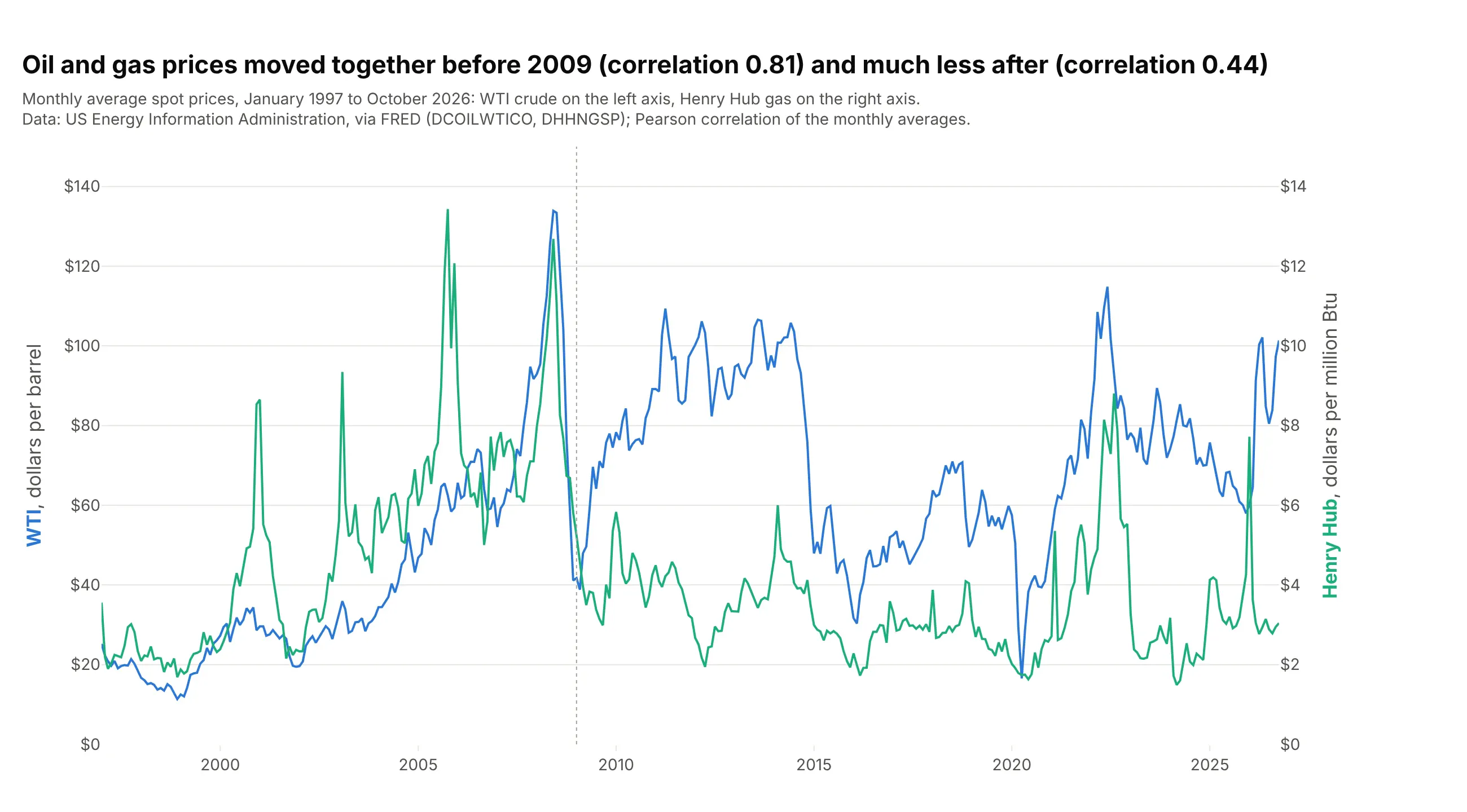
A second y axis puts two series with different units on one chart, here oil in dollars per barrel and gas in dollars per million Btu. Their monthly averages had a correlation of 0.81 from 1997 to 2008 and 0.44 from 2009 on, and the chart shows the split. The catch is that the crossings and the apparent gap depend entirely on how you scale each axis, so state both ranges and don't read meaning into where the lines cross; indexing (way 4) or small multiples (way 5) are safer. In Plotly, make_subplots(specs=[[{"secondary_y": True}]]) and secondary_y=True on the second trace.

Prompt: Get daily WTI (DCOILWTICO) and Henry Hub gas (DHHNGSP) spot prices from FRED (US EIA) since 1997 and resample to monthly averages. Make a plotly chart with make_subplots(specs=[[{"secondary_y": True}]]): WTI in blue on the left axis ($0-$150), Henry Hub in green on the right axis ($0-$15), each axis title colored like its line. Print the correlation before and after 2009 and put both in the title.

11. A row of sparklines

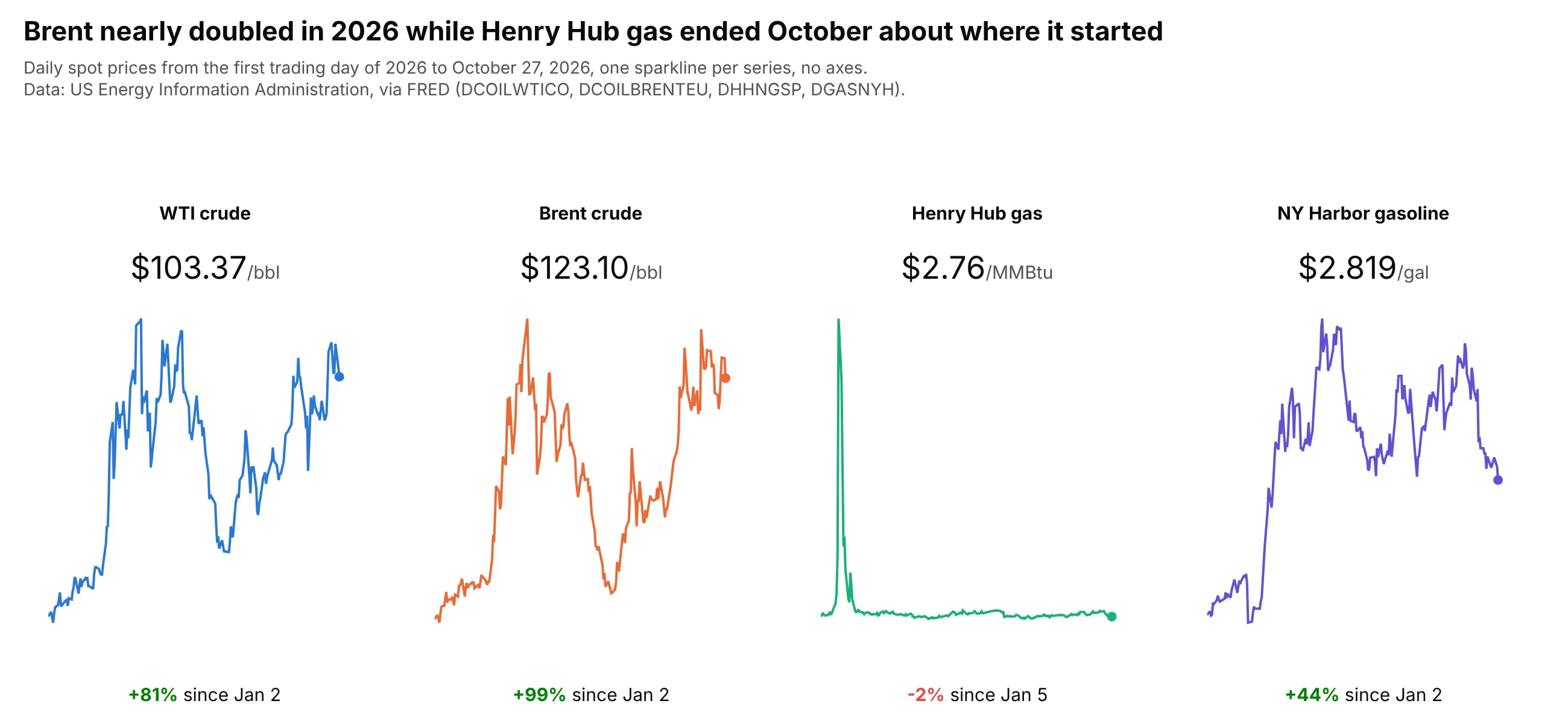
A sparkline is a small line with no axes next to a number, the way dashboards and app headers show trends. This row shows that Brent nearly doubled in 2026, up 99% from January 2 to October 27, while Henry Hub gas ended almost where it started after its January spike. Each one is a subplot with fig.update_xaxes(visible=False) and fig.update_yaxes(visible=False), a dot on the last value, and the numbers as annotations.

Prompt: Get 2026 daily spot prices from FRED for WTI (DCOILWTICO), Brent (DCOILBRENTEU), Henry Hub gas (DHHNGSP) and New York Harbor gasoline (DGASNYH). Make a plotly figure with make_subplots(rows=1, cols=4), one small line per series with hidden axes and a dot on the latest price. Above each, the series name and latest price in large type; below, the percent change since the first trading day in green or red.

12. Percent change from a year earlier

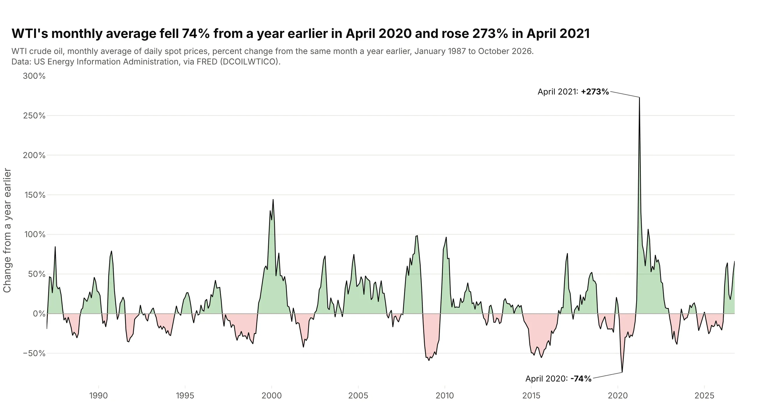
Plotting the change from the same month a year earlier removes the seasonal pattern and the long-run level, so booms and busts look the same size whatever the price. WTI's monthly average was 74% below a year earlier in April 2020 and 273% above it in April 2021, the same crash seen from both sides. Compute monthly / monthly.shift(12) - 1 and fill above and below zero in different colors with fill="tozeroy" on clipped copies of the series.

Prompt: Get daily WTI crude oil spot prices from FRED (DCOILWTICO, US EIA) since 1986, resample to monthly averages and compute the percent change from the same month a year earlier. Make a plotly line chart of it with a black line, green fill="tozeroy" above zero and red below (using clipped copies of the series), a gray zero line and the largest rise and fall labeled.