Chris Parmer

November 9, 2026

Tornado Charts - A Complete Guide

TL;DR

A tornado chart shows how much one model output, such as a project's cost or value, moves when each input is set to a low and a high value while every other input stays at its base case. Each input gets a horizontal bar centered on the base case, and the bars are sorted so the widest is on top, which gives the chart its funnel shape.
Tornado charts are also known as tornado diagrams and tornado plots, and the method behind them is one-way or one-at-a-time sensitivity analysis. They are similar to spider plots, which draw each input's whole range as a line, to bar charts and diverging (Likert) charts in shape, and to waterfall charts when inputs change one after another.
Decision analysts, oil and gas engineers, energy planners, drug developers and health economists use them to decide which assumptions deserve more data before a decision. They can't show interactions between inputs or inputs that move together, so a wide bar is a reason to look closer, not a forecast.
You can make a tornado chart with Plotly from two go.Bar traces with orientation="h" and base= set to the base-case output. A short helper function is below.

What is a tornado chart?

Tornado charts look like this:

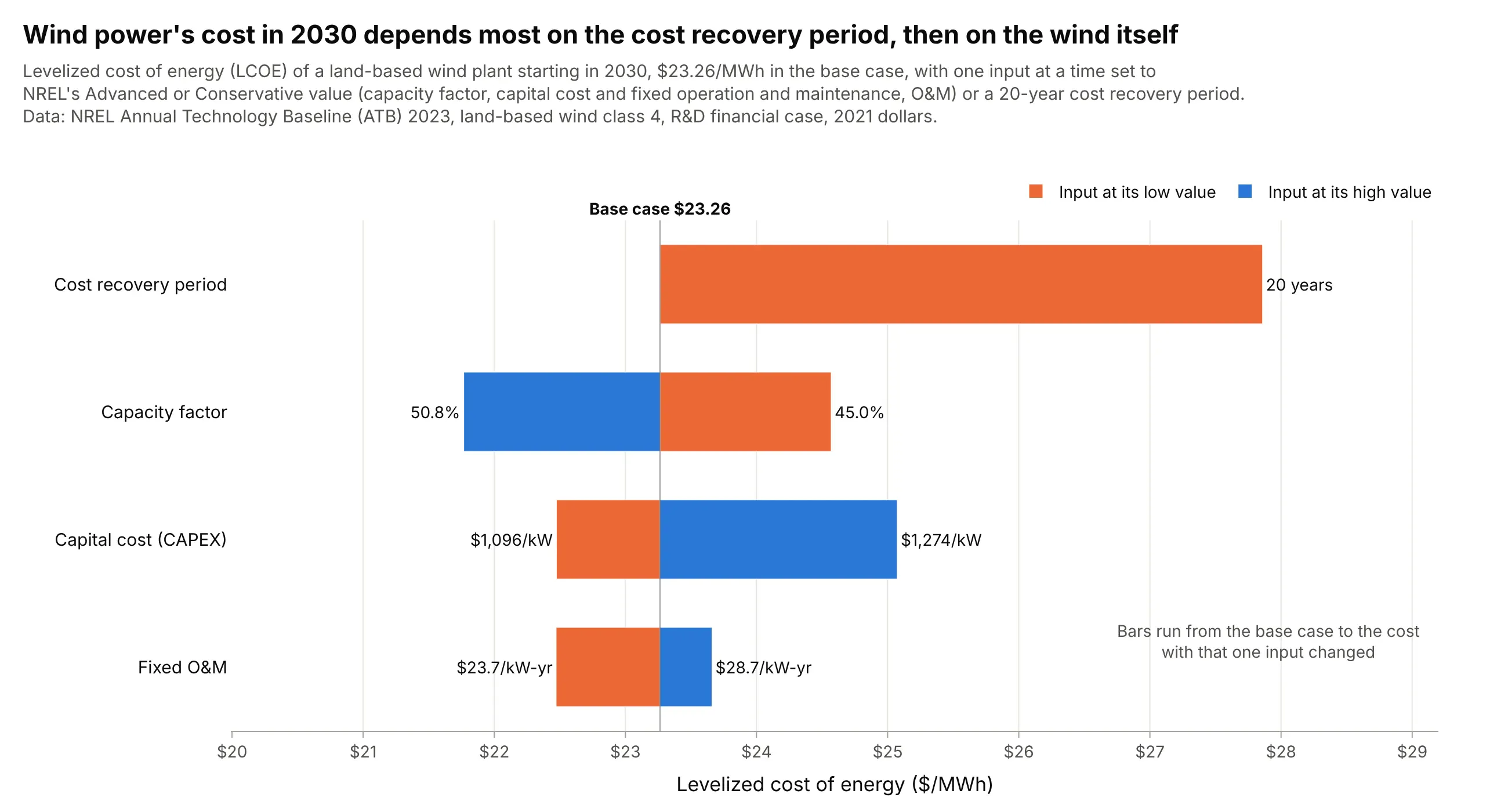
Tornado chart of the levelized cost of energy of a land-based wind plant starting in 2030, base case 23.26 dollars per megawatt-hour: a 20-year cost recovery period raises it to 27.86 in an orange bar to the right only; capacity factor runs from 21.77 at 50.8% in blue to 24.57 at 45.0% in orange; capital cost from 22.47 at 1,096 dollars per kilowatt to 25.07 at 1,274; fixed O&M from 22.47 to 23.66

Data: National Renewable Energy Laboratory (NREL), Annual Technology Baseline (ATB) 2023, land-based wind, resource class 4.

How do you read a tornado chart? In the example above, notice these things:

The output is the levelized cost of energy (LCOE), the price per megawatt-hour (MWh) a wind plant needs to cover its costs over its life. The black line is the base case, $23.26/MWh, computed with NREL's middle (Moderate) value of every input.
Each row changes one input and nothing else. Orange bars show the cost with the input at its low value and blue bars with it at its high value, and the input values sit at the bar ends: a capacity factor (the share of the year's maximum output the plant delivers) of 45.0% instead of 47.5% raises the cost to $24.57.
The rows are sorted by swing, the distance between the two ends. Recovering the capital over 20 years instead of 30 adds $4.59, more than the $2.80 swing of the capacity factor or the $2.60 swing of the capital cost (CAPEX, capital expenditure).
The top bar has only one side, because the base case already uses the longer of the two periods. A short bar, like fixed operation and maintenance (O&M) at $1.19, is an input that matters less for this decision.

It's often used for charts like these:

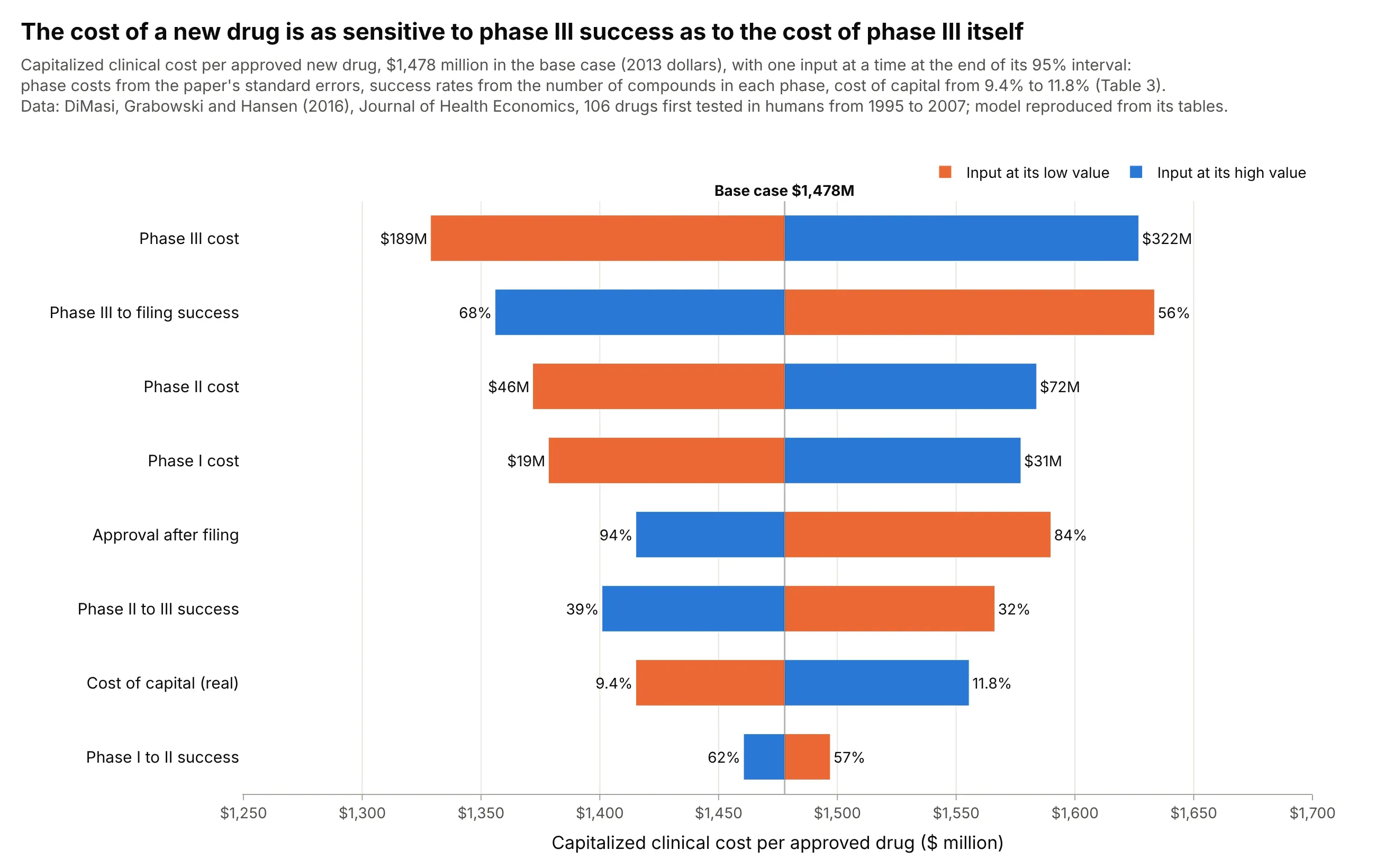
Tornado chart of the capitalized clinical cost per approved new drug, base case 1,478 million dollars: phase III cost between 189 and 322 million moves it from 1,329 to 1,627; phase III to filing success between 56% and 68% moves it from 1,633 to 1,356; then phase II cost, phase I cost, approval after filing, phase II to III success, cost of capital between 9.4% and 11.8%, and phase I to II success with the narrowest bar

Drug development cost in pharma. In a model rebuilt from DiMasi, Grabowski and Hansen's 2016 study, the uncertainty in phase III's success rate moves the cost per approved drug almost as much as the uncertainty in phase III's cost, $278 million against $298 million. Data: DiMasi, Grabowski and Hansen (2016), Journal of Health Economics.

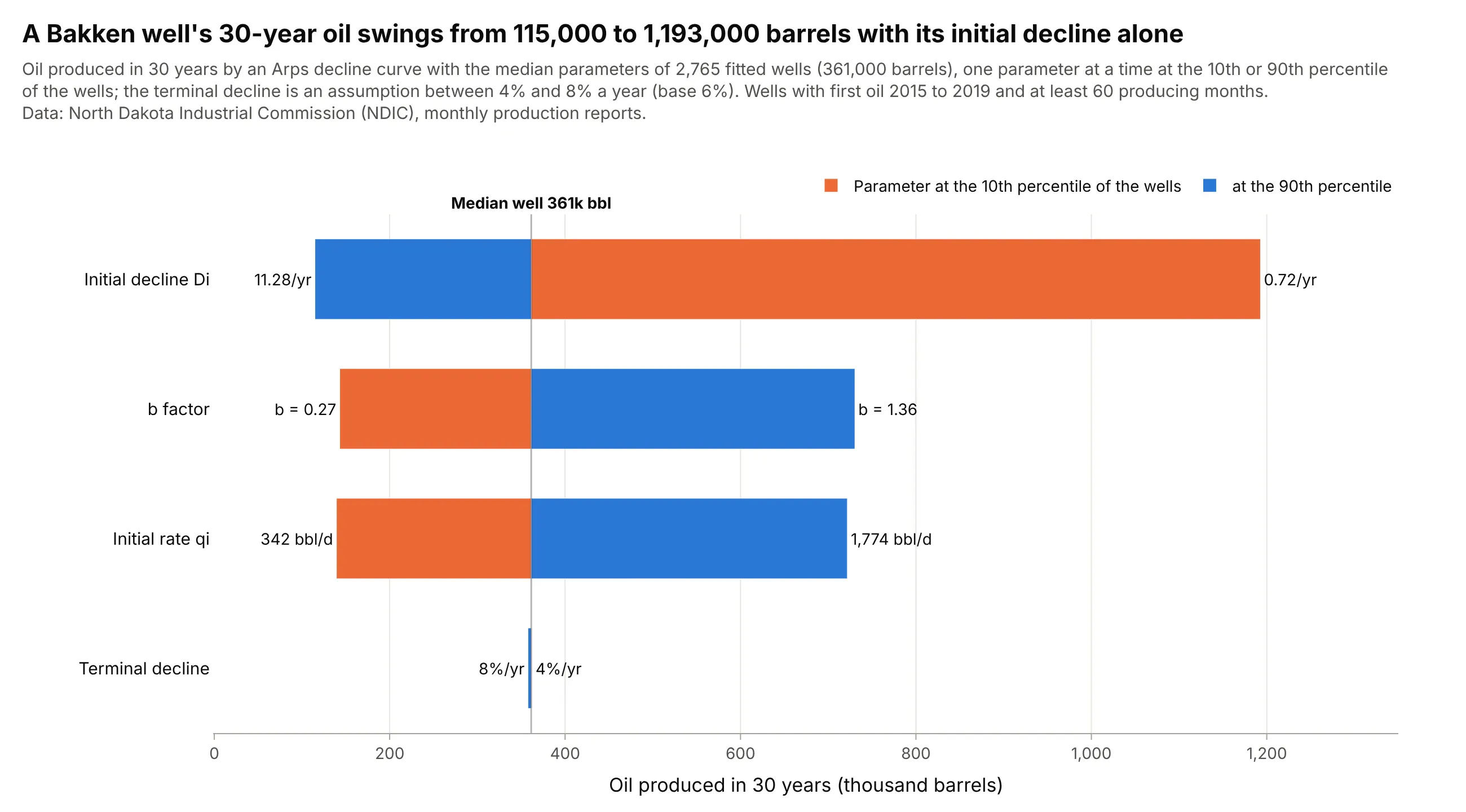
Tornado chart of a Bakken well's 30-year oil, base case 361 thousand barrels for the median parameters of 2,765 wells: the initial decline at its 10th and 90th percentile moves it from 1,193 thousand to 115 thousand; the b factor from 143 to 730 thousand; the initial rate from 139 to 722 thousand; the terminal decline between 4% and 8% a year barely moves it

Reserves and well economics in oil and gas. Setting each Arps decline parameter of a North Dakota shale well to the 10th or 90th percentile of 2,765 real wells shows the initial decline rate moves 30-year oil the most, from 115,000 to 1,193,000 barrels. Data: North Dakota Industrial Commission (NDIC), monthly production reports.

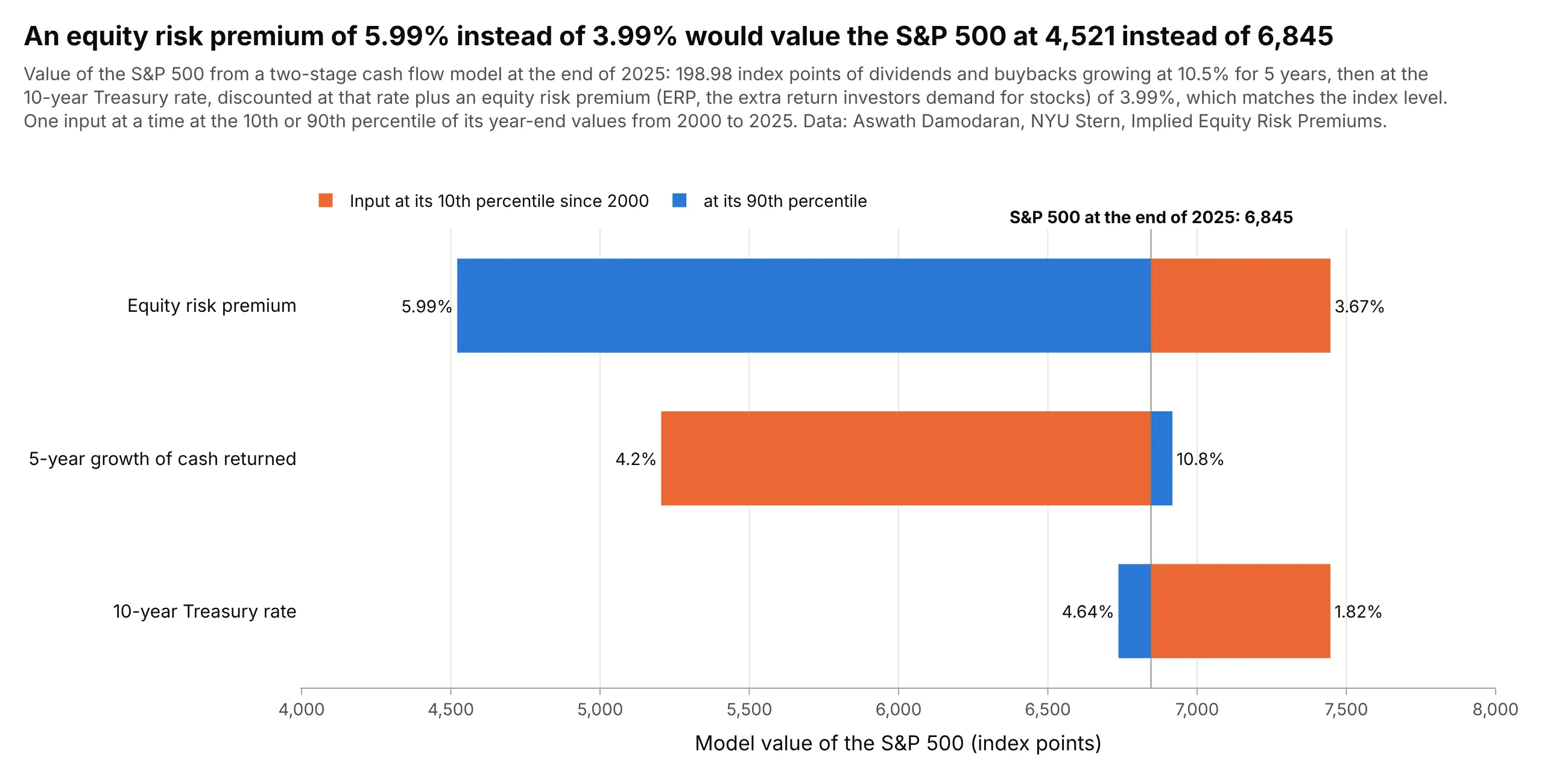
Tornado chart of a two-stage cash flow model of the S&P 500 at the end of 2025, base 6,845: the equity risk premium between 3.67% and 5.99% moves it from 7,448 to 4,521; the 5-year growth of cash returned between 4.2% and 10.8% from 5,204 to 6,919; the 10-year Treasury rate between 1.82% and 4.64% from 7,448 to 6,735

Valuation in finance. In a two-stage cash flow model of the S&P 500, an equity risk premium (ERP, the extra return investors demand for owning stocks) of 5.99% instead of 3.99% would value the index at 4,521 instead of 6,845. Data: Aswath Damodaran, NYU Stern, Implied Equity Risk Premiums.

A short history

Tornado diagrams come from decision analysis, the practice of structuring large, uncertain business decisions with models and probabilities, and Ronald Howard's 1988 review of the field, "Decision Analysis: Practice and Promise" in Management Science, already treats them as a standard tool for finding the uncertainties that matter. Ted Eschenbach's 1992 paper "Spiderplots versus Tornado Diagrams for Sensitivity Analysis" describes tornado diagrams as the decision analysts' tool and spider plots as the engineering economists', and recommends using both. Spreadsheet risk tools then made them routine: Oracle Crystal Ball has a Tornado Analysis tool and @RISK draws tornado graphs from its simulations. Project managers know them from the PMBOK Guide (A Guide to the Project Management Body of Knowledge), and health economists use them to show one-way sensitivity analyses of cost-effectiveness models (Encyclopedia of Medical Decision Making, 2009). The name comes from the shape: wide at the top, narrow at the bottom.

How a tornado chart is built

A tornado chart is the picture of a simple experiment run on a model. Knowing the steps tells you what the chart can and can't claim.

1. A model and a base case

You need a model that turns inputs into one output: a cost formula, a discounted cash flow, a reservoir forecast, an engineering equation. The base case is the output with every input at its best estimate. In the wind example the model is NREL's LCOE formula, the fixed charge rate (the yearly share of the capital cost that pays back investors) times the capital cost, plus fixed O&M, divided by the energy produced per kilowatt in a year, and the base case is $23.26/MWh.

2. One input at a time

Each bar comes from two runs of the model. Set one input to its low value with every other input at its base value, run the model, then do the same with the input at its high value. Here is the capacity factor bar:

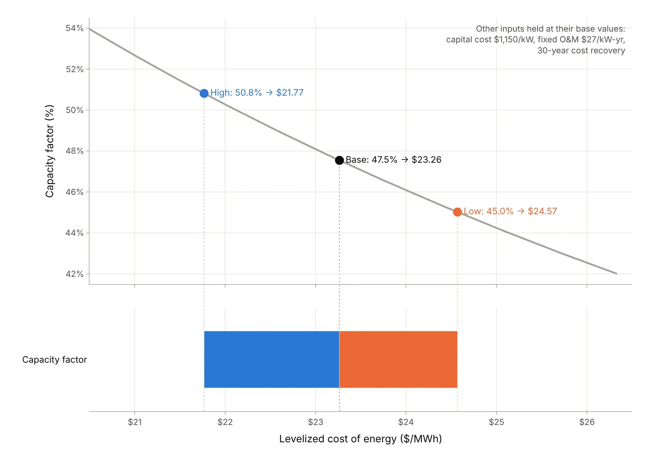
The wind LCOE as a function of capacity factor, a gray curve falling from about 26.3 dollars at 42% to 20.5 at 54%, with three points marked: high 50.8% gives 21.77, base 47.5% gives 23.26, low 45.0% gives 24.57; dotted lines drop from each point to a single tornado bar below that runs from 21.77 in blue to 24.57 in orange

Data: NREL ATB 2023, land-based wind class 4; the other inputs are held at their base values.

Crystal Ball's documentation describes the same method: the tool "freezes the other variables at their base values" and is "also known as one-at-a-time perturbation or parametric analysis". With n inputs, the chart needs 2n + 1 runs of the model, which is why it is the first sensitivity analysis people run on a spreadsheet.

3. Low and high values: P10 and P90

The bars are only as fair as the ranges behind them. A common choice is the 10th and 90th percentile of each input's uncertainty (called P10 and P90), so every bar covers the same 80% range of belief; Crystal Ball lets you choose the percentiles. Other ranges in this guide are a published low and high scenario (NREL's Advanced and Conservative values), a 95% confidence interval from a study's standard errors, the 10th and 90th percentile across 2,765 real wells, and the design range of an engineering variable. Say on the chart which one you used. In the oil and gas industry, watch the direction: reserves engineers call the high estimate P10 (a 10% chance of more), the opposite of a statistician's 10th percentile.

Giving every input the same percentage, such as plus and minus 10%, answers a different question. It ranks the inputs by elasticity, how strongly the output responds to a proportional change, rather than by how uncertain they are. Example 5 below shows the wind model both ways.

4. Sort by swing, and color by the input's end

The swing is the absolute difference between the two outputs. Sorting with the widest bar on top is what makes the chart a tornado, and it is the whole point: the reader sees at once which assumptions matter. We color each bar by which end of the input's range produced it (orange for low, blue for high), which shows direction: a high capacity factor lowers the cost, a high capital cost raises it. Crystal Ball's tornado chart does the same, with the upside of each variable in blue and the downside in red.

5. Bars that break the pattern

Three shapes are worth recognizing. A one-sided bar means the base case sits at one end of the input's range, like the 30-year cost recovery period. An asymmetric bar means the output responds nonlinearly: because cost is divided by capacity factor, a 10% lower capacity factor adds 11.1% and a 10% higher one saves 9.1%. A bar with both ends on the same side means the input is non-monotonic: the output rises at both ends, so the "swing" between them is close to zero even though the input matters (the sweep angle in example 4 and x2 below).

6. What a tornado chart can't show

Holding everything else at base leaves out interactions, where one input's effect depends on another's value. The Ishigami function, a standard test of sensitivity methods, is built to show this. With every input at zero, its third input has no effect at all one at a time, yet it explains 24% of the output's variance once all inputs vary together, because it multiplies the first:

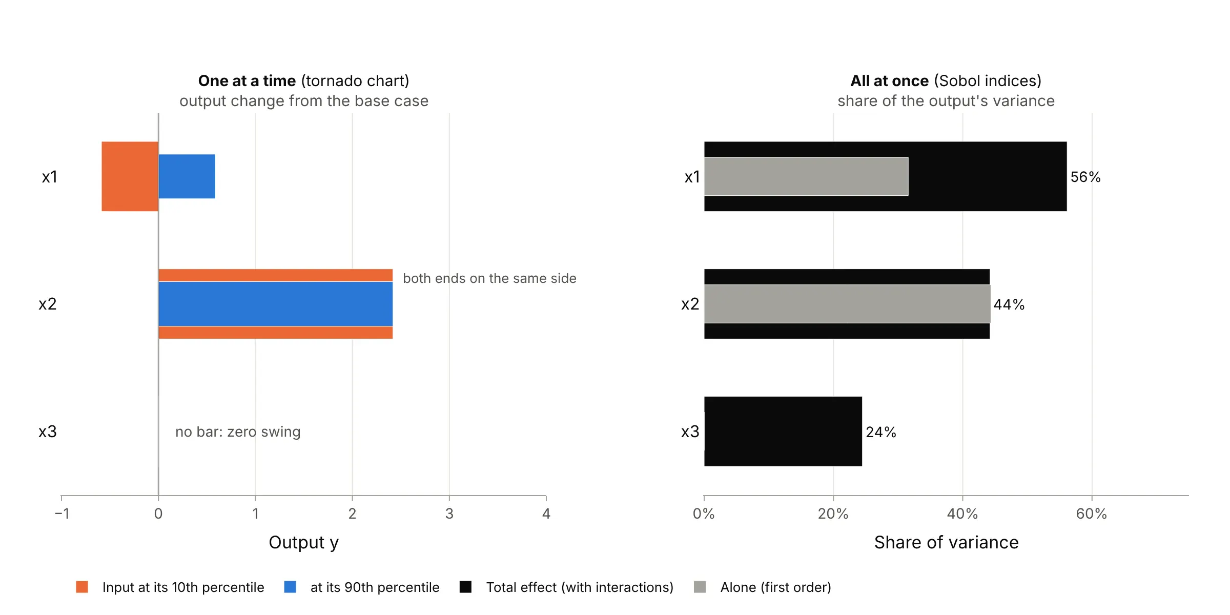
Two panels on the Ishigami test function. Left, a tornado chart from the base case at zero: x1 has bars from -0.59 to +0.59, x2 has both bars on the same side reaching 2.42, x3 has no bar. Right, Sobol variance shares: x1 56% total and 32% alone, x2 44% total and alone, x3 24% total and 0% alone

Data: the Ishigami function (Ishigami and Homma 1990), a theoretical test function, not data; Sobol indices estimated with 200,000 Monte Carlo samples.

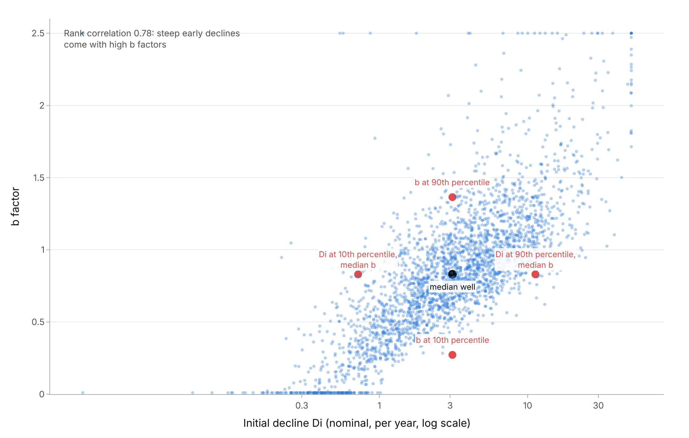
The same goes for inputs that move together. Real Bakken wells with a steep initial decline also have a high b factor (rank correlation 0.78), so the tornado in example 03 pairs values that rarely occur together (see "Another way to see it" under "More tornado chart examples"). And because each bar varies one input, the bars don't add up: putting all four wind inputs at their costlier values gives $32.27/MWh, $0.90 more than the base plus the four bars. When interactions or correlations matter, run a Monte Carlo simulation, which varies every input at once, and rank the inputs by variance-based (Sobol) indices or by the regression coefficients that @RISK's tornado graphs use.

A spider plot is the usual companion. It draws the output against the percent change of each input across its whole range, so you can see the shape of each response, where a line crosses a break-even value, and how far each input can move:

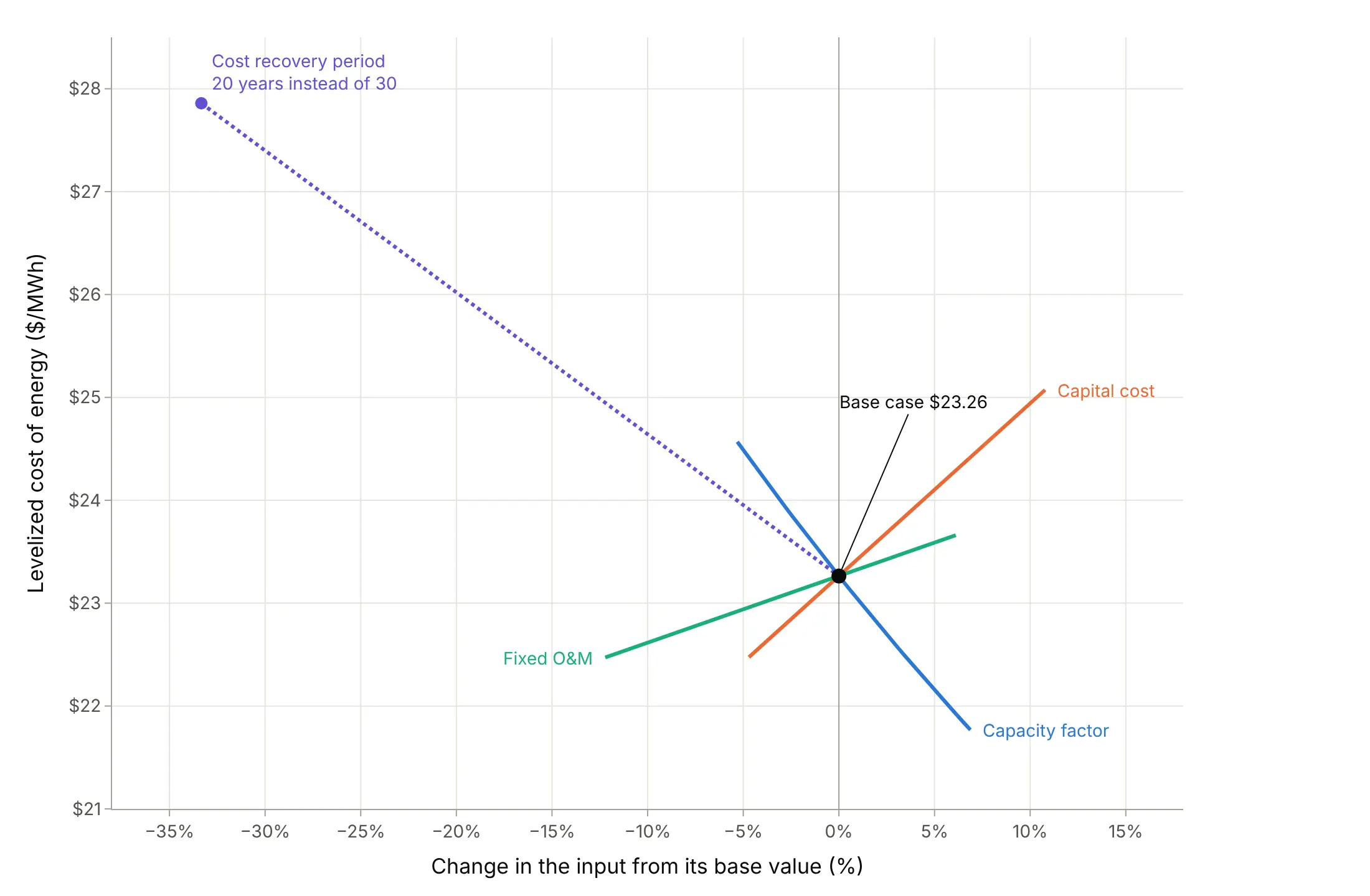
Spider plot of the wind LCOE against the percent change of each input: capital cost rises from 22.47 at -4.7% to 25.07 at +10.8%, capacity factor falls from 24.57 at -5.3% to 21.77 at +6.9%, fixed O&M rises gently from -12% to +6%, and a dotted purple line runs from 27.86 at -33% (a 20-year cost recovery period) to the base case of 23.26 at 0%

Data: NREL ATB 2023, land-based wind class 4.

Alternatives to a tornado chart

Here's the wind cost sensitivity drawn six ways. Some are better for the question, some worse, some just different:

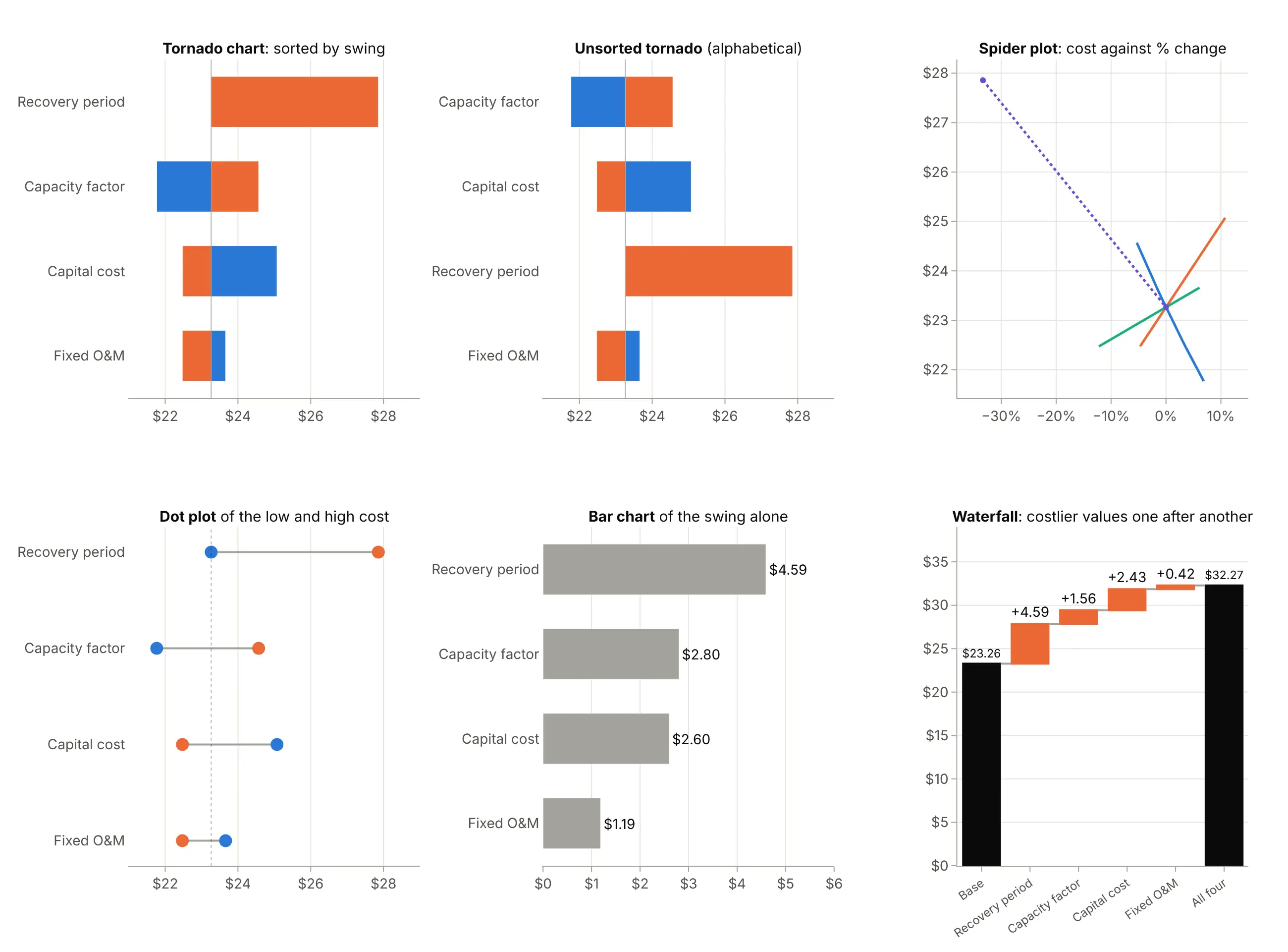
The wind LCOE sensitivity drawn six ways: a tornado chart sorted by swing; the same bars in alphabetical order with the widest bar third; a spider plot of cost against percent change; a dot plot of the low and high cost for each input; a gray bar chart of the swing alone, 4.59, 2.80, 2.60 and 1.19; and a waterfall that applies the costlier value of each input one after another from 23.26 to 32.27

Unsorted tornado (worse). In alphabetical or model order the reader has to hunt for the widest bar, which is the one thing the chart exists to show.
Spider plot (works too, with fewer inputs). It shows each input's full response and where it crosses a threshold, but past five or six lines it becomes hard to read, and inputs whose ranges differ in percent sit at different widths.
Dot plot or dumbbell chart (works too). The low and high outputs as two dots on a line carry the same numbers with less ink, though the base case is easier to miss.
Bar chart of the swing (worse). It ranks the inputs but loses the base case and the direction of each effect.
Waterfall chart (different). Changing the inputs one after another shows how a worst case builds up and includes the interactions, but the size of each step depends on the order you choose.
Diverging (Likert) chart and butterfly chart (different). They look alike, bars running both ways from a center line, but show shares of survey answers or two populations back to back, not sensitivity. Some sources, Wikipedia among them, list "butterfly chart" as another name for a tornado chart; most people use it for the back-to-back chart, as in a population pyramid.

How to make a tornado chart

With AI

ChatGPT, Claude Code, GitHub Copilot, Cursor and other AI tools are excellent at writing Plotly code. Name Plotly in the prompt, and give it the model, the base case and the range for each input, so it computes the bars instead of inventing them:

Make a plotly tornado chart of a wind plant's levelized cost of energy, LCOE = (fcr * capex + fom) * 1000 / (cf * 8760).

- Base case: capex 1150 $/kW, cf 0.475, fom 27 $/kW-yr, fcr 0.0608. Low/high: cf 0.450/0.508, capex 1096/1274,
  fom 23.7/28.65, fcr 0.0774 (20 years) / 0.0608 (30 years, the base).
- Vary one input at a time with the others at base; two go.Bar traces with orientation="h" and base=<base LCOE>.
- Sort by swing with the widest on top; orange for the low input, blue for the high; input values at the bar ends.
- A black line at the base case, labeled with its value. Check: print the table of low, high and swing.

With Plotly Studio

Plotly Studio is a desktop app where you point an AI at a dataset and it builds charts and a Dash app around your questions. Ask for a tornado chart the same way:

From the table of model runs (input, output_low, output_high, base), show a tornado chart sorted by swing with bars starting at the base case, the input values at the bar ends, and a dropdown to switch between the wind, solar and offshore wind cases.

Make a tornado chart in Python or JavaScript

This is the code AI tools write under the hood. Plotly has no dedicated tornado trace, so a tornado chart is two horizontal go.Bar traces whose base is the base-case output and whose x is each output's distance from it, overlaid and sorted by swing. This helper returns a go.Figure, and the code below it runs the one-at-a-time analysis on the wind cost formula:

import pandas as pd
import plotly.graph_objects as go


def tornado(df, base):
    """A tornado chart in Plotly: one row per input, bars from the base case to the low and high outputs."""
    df = df.assign(swing=(df.high - df.low).abs()).sort_values("swing")  # Plotly draws the last row on top
    fig = go.Figure([
        go.Bar(y=df.input, x=df.low - base, base=base, orientation="h", name="Input at its low value",
               marker_color="#eb6834", text=df.low_text, textposition="outside", cliponaxis=False),
        go.Bar(y=df.input, x=df.high - base, base=base, orientation="h", name="Input at its high value",
               marker_color="#2a78d6", text=df.high_text, textposition="outside", cliponaxis=False),
    ])
    fig.add_vline(x=base, line_color="black")
    fig.update_layout(barmode="overlay", template="simple_white")
    return fig


def lcoe(capex, cf, fom, fcr):
    """Levelized cost of energy ($/MWh), NREL ATB's formula for a wind or solar plant."""
    return (fcr * capex + fom) * 1000 / (cf * 8760)


# Land-based wind starting in 2030 (NREL ATB 2023, class 4): base inputs, then each input's low and high value
base_inputs = dict(capex=1150, cf=0.47543, fom=27.0, fcr=0.060774)
ranges = [("Capacity factor", "cf", 0.45018, 0.50812, "45.0%", "50.8%"),
          ("Capital cost", "capex", 1095.9, 1274.0, "$1,096/kW", "$1,274/kW"),
          ("Fixed O&M", "fom", 23.7, 28.65, "$23.7/kW-yr", "$28.7/kW-yr"),
          ("Cost recovery period", "fcr", 0.077414, 0.060774, "20 years", "")]  # fixed charge rate, 20 and 30 years

base = lcoe(**base_inputs)
rows = [dict(input=label, low=lcoe(**{**base_inputs, k: lo}), high=lcoe(**{**base_inputs, k: hi}),
             low_text=lo_text, high_text=hi_text) for label, k, lo, hi, lo_text, hi_text in ranges]
fig = tornado(pd.DataFrame(rows), base)
fig.update_xaxes(title="Levelized cost of energy ($/MWh)")
fig.show()

For your own model, replace lcoe with any function that takes the inputs as keyword arguments, and ranges with your low and high values. The examples in this guide build on the same helper with a title, a legend at the top and a label for the base case.

In JavaScript, plotly.js draws the same chart from the computed outputs:

<div id="chart"></div>
<script src="https://cdn.plot.ly/plotly-4.1.1.min.js"></script>
<script>
  // Levelized cost of land-based wind in 2030 ($/MWh) with one input at a time at its low and high value (NREL ATB 2023)
  const base = 23.26;
  const rows = [  // input, cost with the input low, cost with it high, low and high input values; widest first
    ["Cost recovery period", 27.86, 23.26, "20 years", ""],
    ["Capacity factor", 24.57, 21.77, "45.0%", "50.8%"],
    ["Capital cost", 22.47, 25.07, "$1,096/kW", "$1,274/kW"],
    ["Fixed O&M", 22.47, 23.66, "$23.7/kW-yr", "$28.7/kW-yr"],
  ].reverse();  // plotly.js draws the first row at the bottom
  const bar = (i, name, color) => ({
    type: "bar", orientation: "h", name: name, marker: {color: color}, base: base,
    y: rows.map(r => r[0]), x: rows.map(r => r[i] - base), text: rows.map(r => r[i + 2]),
    textposition: "outside", cliponaxis: false
  });
  Plotly.newPlot("chart", [bar(1, "Input at its low value", "#eb6834"), bar(2, "Input at its high value", "#2a78d6")], {
    width: 900, height: 450, barmode: "overlay", margin: {l: 160},
    xaxis: {title: {text: "Levelized cost of energy ($/MWh)"}, range: [20, 29.5]},
    shapes: [{type: "line", x0: base, x1: base, yref: "paper", y0: 0, y1: 1, line: {color: "black"}}]
  });
</script>

Share it

Every Plotly chart has a Share chart button (the cloud icon in its toolbar) that uploads it to Plotly Cloud and gives you a link. Only you can see it until you change its visibility.

For a live app, put the chart in a Dash app and publish it with the Plotly Cloud CLI. Coding agents can run these commands for you:

pip install "dash[cloud]"
plotly user login
plotly app publish

If your data has to stay in your own cloud or data center, publish to Dash Enterprise instead.

Dos and don'ts

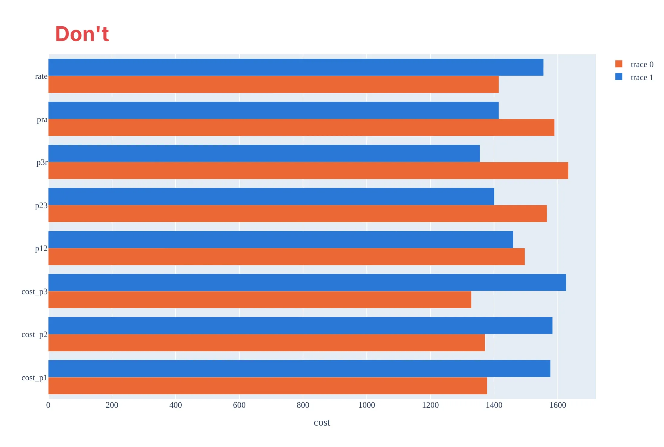
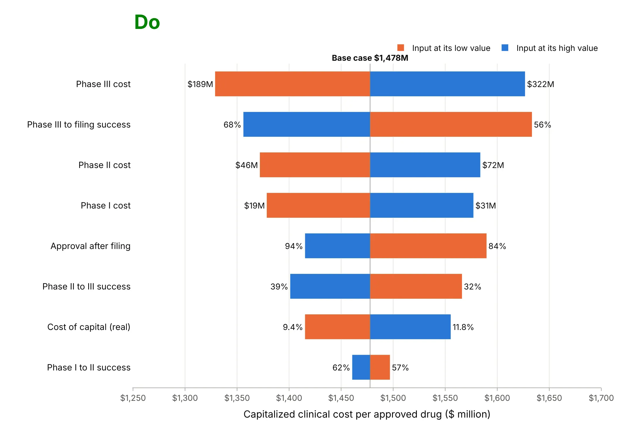
Most of the work in a tornado chart is keeping the base case visible and the order honest. Here is the drug cost model both ways, in the same orange and blue.

Don't draw the low and high outputs as grouped bars from zero, which hides the base case and squeezes every difference into the last few percent of each bar, list the inputs in the order the model defines them, label them with code names, leave out the input values, or keep the default legend and a serif font:

Grouped horizontal bars from zero for eight inputs labeled cost_p1, cost_p2, cost_p3, p12, p23, p3r, pra and rate, every bar between about 1,330 and 1,630 on an axis from 0 to 1,600 titled cost, a legend reading trace 0 and trace 1, a gray background and a serif font

Do start the bars at the base case, sort them by swing, name the inputs in plain words, put the low and high input values at the bar ends, and label the base case:

The same eight inputs as a tornado chart around a base case of 1,478 million dollars, sorted from phase III cost at the top to phase I to II success at the bottom, with the input values at the ends of each orange and blue bar and a legend explaining the colors

Checklist

Say what the base case is, and label its value on the chart.
Say where each low and high value comes from (P10 and P90, a confidence interval, published scenarios), and use comparable ranges for every input.
Sort by swing with the widest bar on top, and keep one color for the low end of an input and one for the high end.
Put the input values at the bar ends, so readers can judge whether the range is reasonable.
Mark one-sided and non-monotonic bars instead of hiding them.

Don't

Present a tornado chart as the probability of an outcome: it shows what each input could do alone, not how likely the result is.
Add the bars together to get a worst case.
Vary inputs that move together (price and volume, decline and b factor) as if they were independent without saying so.
Mix ranges of different kinds (a 95% interval for one input, plus and minus 50% for another) on one chart.

Options to customize

A tornado chart in Plotly is two go.Bar traces plus a line, so these are the options that matter most. The full lists are in the bar trace reference and the horizontal bar charts documentation.

orientation="h": horizontal bars, one row per input on the y axis.
base=: where each bar starts; set it to the base-case output and give x as the distance from it.
barmode="overlay": draw the low and high bars on the same row instead of side by side.
y order or yaxis.categoryorder="array" with categoryarray: sort by swing; Plotly draws the first category at the bottom, so put the widest last.
marker_color: one color for the low end of every input and one for the high end (or color by whether the output goes up or down).
text, textposition="outside" and cliponaxis=False: the input values at the ends of the bars.
fig.add_vline(x=base) with annotation_text: the base-case line and its value.
width on the trace and bargap in the layout: bar thickness; a narrower second trace can show two values on the same side.
customdata and hovertemplate: the input value and the output on hover.
make_subplots(shared_xaxes=True) or shared_yaxes=True: several tornado charts side by side, as in example 2 below.

More tornado chart examples

Five more tornado charts, from energy, pharma and engineering, each with its source, the technique that makes it work and a prompt to rebuild it.

1. A solar farm's site matters more than its cost assumptions

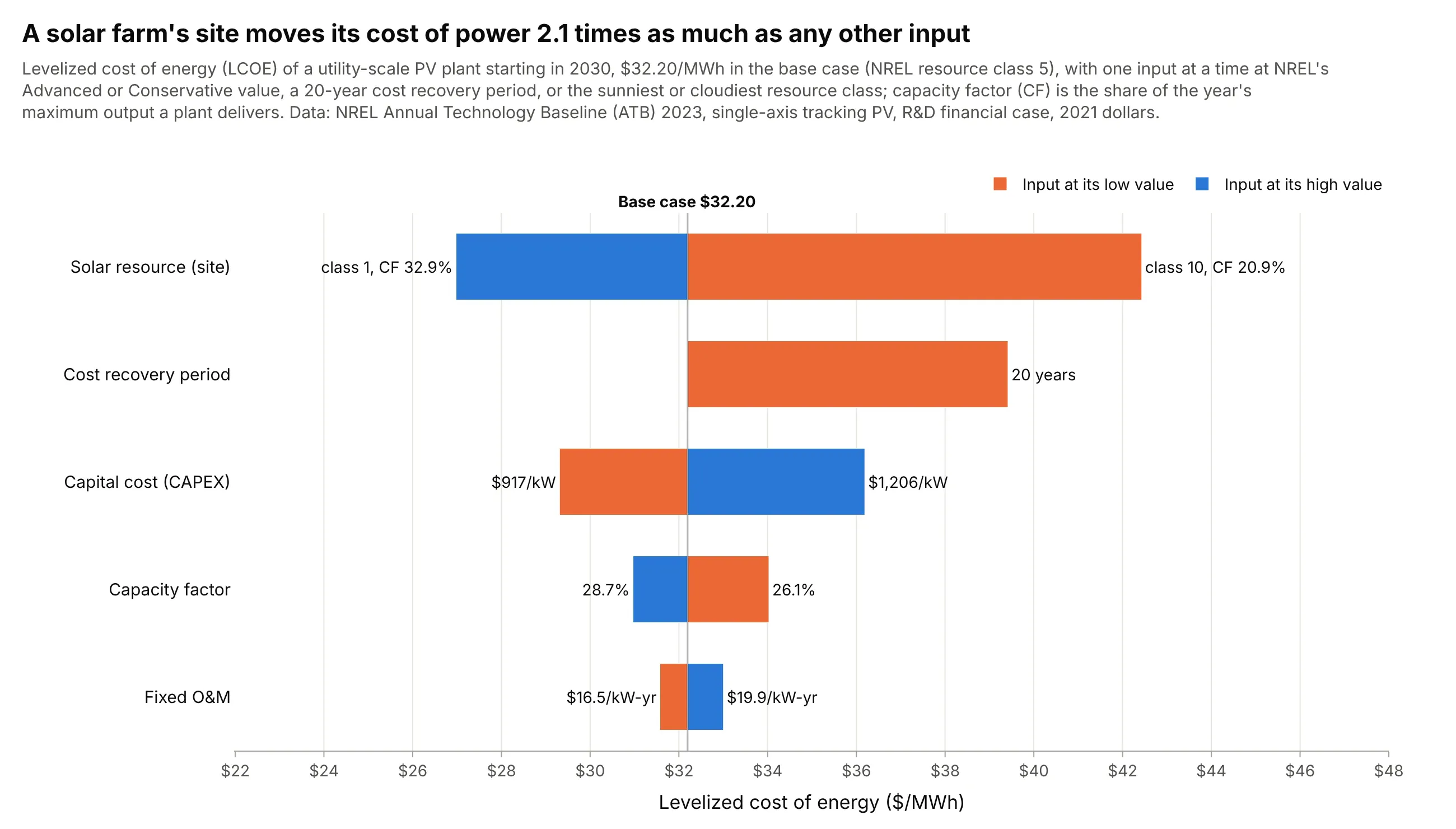
Tornado chart of the levelized cost of a utility-scale solar plant in 2030, base case 32.20 dollars per MWh: the solar resource from class 1 with a 32.9% capacity factor to class 10 with 20.9% moves it from 26.98 to 42.43; a 20-year cost recovery period raises it to 39.42; capital cost 917 to 1,206 dollars per kW from 29.31 to 36.19; capacity factor and fixed O&M bars are narrow

Adding the site to NREL's cost uncertainties puts it on top: moving the same solar plant from NREL's sunniest resource class to its cloudiest raises its cost from $26.98 to $42.43/MWh, a swing 2.1 times that of the next input. Data: NREL Annual Technology Baseline 2023, utility-scale PV.

Tip: put a choice you control (the site) on the same axis as the uncertainties you don't, so the reader can compare them.

Get the data from NREL's Annual Technology Baseline 2023 (OEDI data lake, ATB/electricity/parquet/2023/ATBe.parquet)
and keep utility-scale PV for 2030, R&D financial case (columns: resource_class, scenario, recovery_years, capex_kw,
cf, fom_kw_yr, fcr).

Build a plotly tornado chart of LCOE for class 5 with CAPEX, CF and fixed O&M at their Advanced and Conservative
values, a 20-year cost recovery period, and the capacity factor of class 1 and class 10, sorted by swing.

2. Wind, solar and offshore wind on one percentage axis

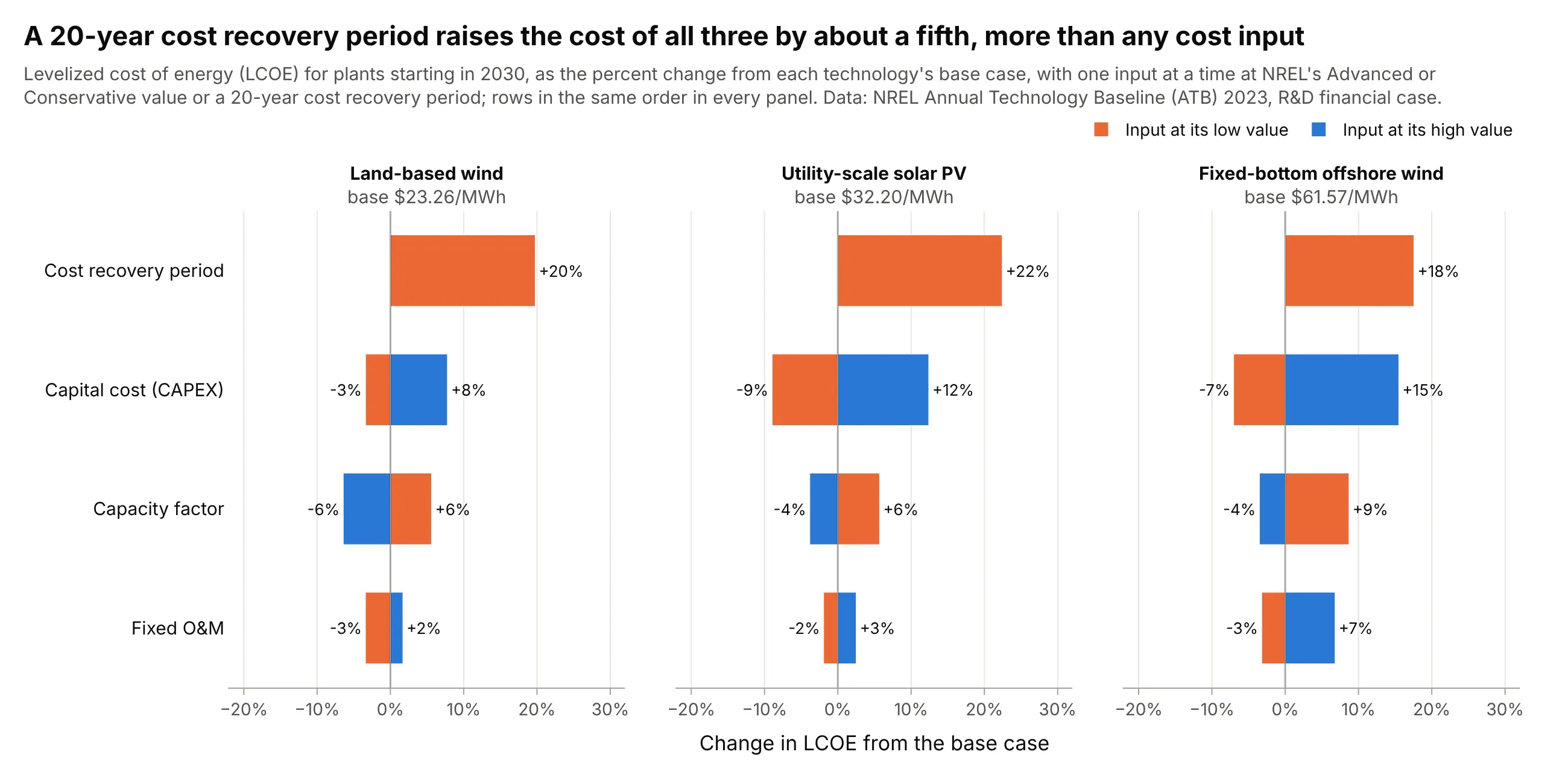
Three tornado charts side by side on a shared axis of percent change in levelized cost: land-based wind (base 23.26), utility-scale solar (32.20) and fixed-bottom offshore wind (61.57), rows in the same order; a 20-year cost recovery period adds 20%, 22% and 18%; capital cost moves them from -3% to +8%, -9% to +12% and -7% to +15%

On a shared percentage axis, a 20-year cost recovery period raises the cost of all three technologies by 18% to 22%, more than any single cost input, while offshore wind's capital cost adds up to 15.5%. Data: NREL Annual Technology Baseline 2023, 2030.

Tip: in small multiples keep the rows in the same order in every panel instead of re-sorting each one, so the eye can compare along a row.

Get the data from NREL's Annual Technology Baseline 2023 (OEDI data lake, ATBe.parquet) for land-based wind class 4,
utility-scale PV class 5 and fixed-bottom offshore wind class 3 in 2030 (columns: technology, scenario,
recovery_years, capex_kw, cf, fom_kw_yr, fcr).

Build three plotly tornado charts with make_subplots(cols=3, shared_yaxes=True), each as the percent change from its
own base LCOE, with the same row order in every panel and the base value in each panel title.

3. Why the cost of a new drug rose 145%

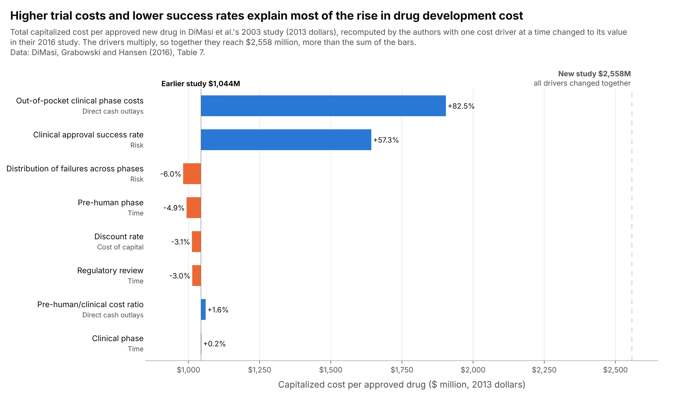
One-sided tornado chart starting at the earlier study's 1,044 million dollars per approved drug: out-of-pocket clinical phase costs at their new values raise it 82.5% and the lower clinical approval success rate 57.3%, while the distribution of failures, pre-human time, discount rate and regulatory review time each lower it 3% to 6%; a dashed line marks the new study's 2,558 million with all drivers changed together

The authors of the 2016 study ran their own one-at-a-time analysis: higher clinical trial costs alone would have raised the earlier study's $1,044 million by 82.5%, and the lower success rate by 57.3%. Together the drivers reach $2,558 million, more than the bars add up to, because they multiply. Data: DiMasi, Grabowski and Hansen (2016), Table 7.

Tip: when each input moves from one known value to another instead of across a range, draw one-sided bars and mark the all-inputs result as a reference line.

Get the data from DiMasi, Grabowski and Hansen (2016), "Innovation in the pharmaceutical industry: New estimates of
R&D costs", Journal of Health Economics, Table 7 (columns: category, factor, total_musd, pct_change), with the prior
study's 1,044 and the new study's 2,558 million.

Build a plotly tornado chart with one bar per factor starting at 1,044 (base=1044), blue for increases and orange
for decreases, the published percent change at each bar end, and a dashed line at 2,558.

4. Five of ten design variables decide a light aircraft's wing weight

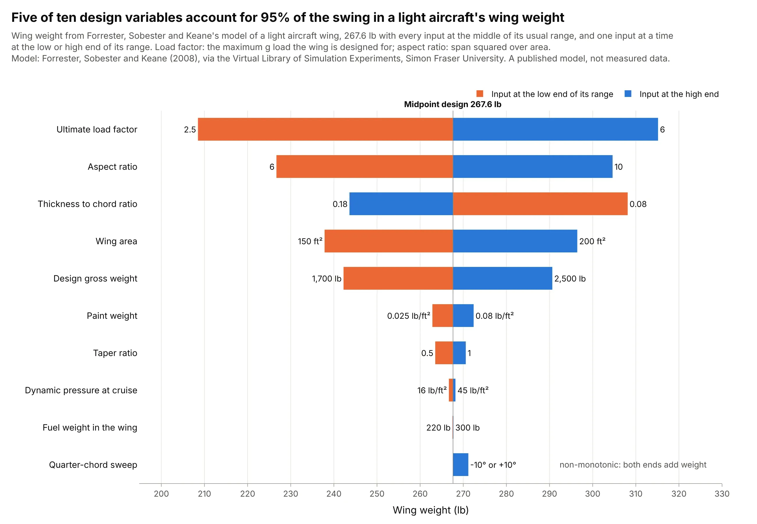
Tornado chart of a light aircraft wing's weight with ten design variables, base 267.6 lb at the middle of every range: ultimate load factor 2.5 to 6 moves it from 208 to 315 lb, aspect ratio 6 to 10 from 227 to 305, thickness to chord ratio from 308 to 244, wing area 150 to 200 square feet from 238 to 296, design gross weight 1,700 to 2,500 lb from 242 to 291; four inputs barely move it; sweep's bar sits on one side because both minus 10 and plus 10 degrees add weight

In a published engineering model of a light aircraft wing, the load factor the wing is designed for swings its weight by 107 lb, and the top five of ten variables account for 95% of the summed swings. Sweep is non-monotonic, adding 3.6 lb at either end of its range. Data: Forrester, Sobester and Keane (2008), via the Virtual Library of Simulation Experiments, Simon Fraser University.

Tip: with many inputs, keep the long tail of short bars: it is the evidence that those inputs can be fixed at their base values.

Get the data from the Virtual Library of Simulation Experiments (sfu.ca/~ssurjano/wingweight.html): the wing weight
function of Forrester, Sobester and Keane (2008) with its 10 inputs and their usual ranges.

Write the function in Python, evaluate it with every input at its midpoint and then one input at a time at each end
of its range, and build a plotly tornado chart sorted by swing with the input values at the bar ends.

5. The same wind model with every input moved by 10%

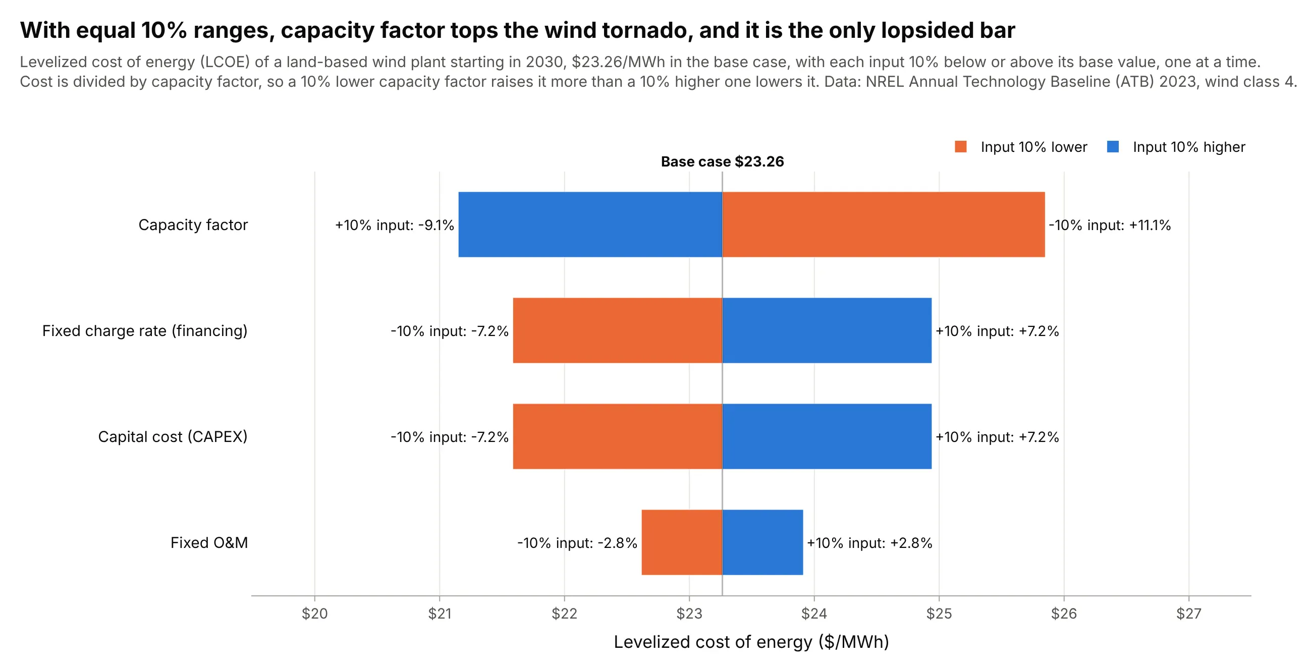
Tornado chart of the wind LCOE with each input 10% lower or higher: capacity factor on top with +11.1% for a 10% lower value and -9.1% for a 10% higher one, then fixed charge rate and capital cost at plus and minus 7.2% each, and fixed O&M at plus and minus 2.8%

With every input moved by the same 10%, capacity factor tops the chart and its bar is lopsided, +11.1% against -9.1%, because the cost is divided by it. The ranking now measures how the formula responds, not how uncertain each input is, which is why it differs from the chart at the top of this guide. Data: NREL Annual Technology Baseline 2023, land-based wind class 4.

Tip: if you use equal percentage ranges, say so in the title, because readers will assume the bars rank the uncertainties.

Get the data from NREL's Annual Technology Baseline 2023 (OEDI data lake, ATBe.parquet), land-based wind class 4,
2030, Moderate scenario, R&D financial case (columns: capex_kw, cf, fom_kw_yr, fcr).

Build a plotly tornado chart of LCOE with each input 10% below and above its base value, the output change in percent
at each bar end, sorted by swing.

Another way to see it: example 03's decline parameters plotted against each other show why a tornado chart can mislead when inputs move together. The red points are the combinations the tornado chart used, and two of them sit where almost no real well is:

Scatter plot of the fitted initial decline Di on a log axis against the b factor for 2,765 Bakken wells, rising together with a rank correlation of 0.78; the median well is a black point and the four red points used in the tornado chart sit at the 10th and 90th percentile of one parameter with the other at its median, two of them away from the cloud