Mina Mirzaei

July 26, 2023

How Polars Can Help You Build Fast Dash Apps for Large Datasets

Working in the world of data visualization can feel like the average data size keeps growing exponentially but compute power stays the same. While that may be true, we have to ask ourselves: are we actually running in the most optimal way?

There are many ways to accomplish this with Dash: Leveraging tooling or strategies including caching and memorization, minimizing data transfer over the network, and using partial property updates are just a few. We always recommend profiling an application before trying to optimize it: Premature optimization can cost weeks or even months of unnecessary labor. So choose the right fit for each use case.

In Professional Services at Plotly, we frequently encounter use cases with large datasets. Many of these applications require bespoke architectures and there is no complete “one size fits all” data format or database system for any application.

One strategy that has gained significant popularity in recent years is to leverage a memory-mapped data architecture, and in Python pairing Parquet files with a tool like Vaex or Polars is a fantastic strategy to accomplish this.

A recent Professional Services project for an equity firm led to our employment of this system as part of an application build, which paired well with the Dash framework and the Dash Enterprise deployment stack.

It might make sense to look into a memory-mapped data architecture for your Dash application if you have completed profiling your application and are observing some common performance problems:

Callbacks in the app taking very long or just timing out.
Maxing out RAM and CPU in the deployment environment, and upgrading your machine is not a viable option.
Directly reading data from a SQL warehouse that was not intended to be the back-end for a real time web application and can’t be modified to accommodate this demand.

In this article, I will go through how we accomplished this in a production environment using Polars, and describe how Polars could be leveraged into your large data Dash application architecture. We’ll also review a sandboxed use case of Polars and Dash in an open-source Dash application, whose source code is available in our Github: This application uses a dataset with 65 million rows and 25 columns, and illustrates other tools and techniques like Datashader and aggregation to support visualization of that data in a browser window.

What is Polars?

Polar Bear

Polars is a dataframe query engine implemented in Rust with a Python API, it’s a great pandas alternative for when your data starts reaching millions of entries in size.

The underlying data frames in Polars are based on the Apache Arrow format, and with a Rust backend. Rust is the up-and-coming favorite coding language of performance-minded programmers that promises to be fast and memory efficient.

Why is Apache Arrow good for large datasets?

To quote the Apache Org FAQ, Arrow is an “in-memory columnar format, a standardized, language-agnostic specification for representing structured, table-like datasets in-memory.”

One great thing about Apache Arrow datasets is that there’s no serialization and deserialization between on-disk and in memory representation of them. This makes memory-mapped Arrow files super fast to read.

Memory mapping is holding a representation of a file in memory to increase I/O efficiency. This would be challenging or counter productive with large datasets that are bigger than RAM size but with virtual memory on an SSD disk, and no deserialization, memory mapped Arrow files are fast to read with very little memory footprint.

Another useful big data aspect of Arrow files is that they are columnar, so unlike a CSV file where you have to hold an entire row of data in memory just to access one single column, you can efficiently just read in columns you need. With wide datasets, this makes a noticeable difference in the memory footprint.

There’s a brilliant explanation of why Apache Arrow is great at handling large data in this article by one of the cofounders of the Apache Arrow project.

Polars lazy vs eager computations

Cartoon Turtle

Polars will handle your data in one of two ways.

Let’s say you want to read from a parquet file. This method will instantly load the parquet file into a Polars dataframe using the polars.read_parquet() function. This will “eagerly” compute the command, taking 6 seconds in my local jupyter notebook to run. During this time Polars decompressed and converted a parquet file to a Polars dataframe.

Import polars a pl 
df = pl.read_parquet("data/fhvhv_data.parquet")

But if I use scan_parquet, the runtime is zero. What happened here?

ldf = pl.scan_parquet("data/fhvhv_data.parquet")

Well, Polars didn’t actually run any computations; it's now constructed a lazyframe based on my parquet file and is waiting for us to tell it when it’s time to collect the data, utilizing lazy loading!

df = ldf.collect()

Now when I use the collect method, data is being read from the parquet file and constructed into a Polars dataframe. This is a very powerful concept: we can build a lazyframe from all sorts of data loading and wrangling logic, and collect our data only when we need it.

Polars expressions and data wrangling

Polars handles data wrangling with expressions. Expression in the Polars are like functions that can be chained together and applied to a dataframe or series. When you chain a bunch of expressions and apply it to a dataset, Polars will take care of parallelizing wherever possible to run as fast as possible.

It’s recommended you use lazyframes wherever possible to allow Polars to optimize on the entire process from start to end. The Polars API is easy to use once you learn the basics, it’s pretty intuitive what a Polars query is supposed to do. I’ve put together a notebook that can help you jumpstart using Polars. I also highly recommend checking out the Polars user guide.

How to use Polars in a Dash application

If you have large amounts of structured data in a data lake, chances are you have parquet files. Parquet is another Apache project and also a columnar data type. The big difference between parquet and Arrow is that parquet files are compressed and optimized for storage. This is a good article on the differences between Arrow and parquet if you’re curious for more, or to help you decide which file type makes sense for your application.

Building an Arrow file from parquet files can be as simple as a few lines of code.

import polars as pl
df = pl.read_parquet("data/fhvhv_data.parquet")
df.write_ipc("data/fhvhv_data.Arrow")

Store this Arrow file in the Dash Enterprise Persistent Filesystem for a low maintenance, fast performing large data application.

Just note that depending on the nature of the underlying data, you may need to set up a data hydration process that periodically updates your Arrow file. This can be done with a scheduled task running on Celery. Also note that this hydration part will be the most memory consuming part of your Dash application as decompressing parquet files takes memory, so only do when necessary.

There’s plenty of other IO support with Polars to read in from: Avro, CSV, and many more.

Now that we have our data reading set up, let’s go over some good use cases of Polars in Dash apps. We want to utilize what makes Polars fast and efficient by using Arrow files and lazy API.

This sample project showcases how to do this, and we’ll be walking through the code from this sample app as part of this blog. Always refer to the original Polars documentation for more detailed usage guides. This app uses the NYC taxi data and we want to enable a user to browse through this data in a Dash app, filter and select what they want and then visualize some features in scatter plots.

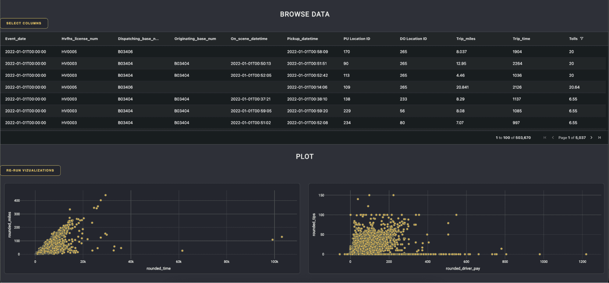
So we have two main challenges: browsing large data sets then visualizing it. Let’s go over these two functions and how to utilize Polars in each case.

Polars in a Dash AG Grid table with infinite scroll

Our data set size is 65 million rows and 25 columns.

We can use a Dash AG Grid with infinite scroll to load only one page at a time in combination with a column selection modal to allow the user to add or remove columns they don’t want to see. Remember we are dealing with columnar data, not row based data, so this little modification can really improve performance.

By storing the data in an IPC Arrow file, we can use Polars in the callbacks for these applications to filter and select the necessary data in a memory efficient way.

The components here are a list of checkboxes for the user to choose which columns to view and then hit an apply button:

dmc.Container(
           [
               *(
                   dmc.Checkbox(
                       label=col,
                       id={"type": "checkbox", "field": col},
                   )
                   for col in all_columns
               ),
               html.Button(
                   "apply",
                   id="apply-bttn",
               ),
           ],
       ),

A Dash AG Grid with infinite row mode:

dag.AgGrid(
           id="infinite-grid",
           rowModelType="infinite",
           enableEnterpriseModules=True,
           columnDefs=layout_utils.generate_column_defintions(),
           pagination=True,
           paginationPageSize=100,
           className="ag-theme-alpine-dark",
           defaultColDef={"filter": True},
       ),

A dcc Store to save the current state of the filter model (more on why we do this in the next part):

dcc.Store(id="filter-model"),

AG Grid with infinite scroll mode, sends a request to the server with a filter model to be applied. We can translate this filter model to Polars expressions:

def parse_column_filter(filter_obj, col_name):
   """Build a polars filter expression based on the filter object"""
   if filter_obj["filterType"] == "set":
       expr = None
       for val in filter_obj["values"]:
           expr |= pl.col(col_name).cast(pl.Utf8).cast(pl.Categorical) == val
   else:
       if filter_obj["filterType"] == "date":
           crit1 = filter_obj["dateFrom"]


           if "dateTo" in filter_obj:
               crit2 = filter_obj["dateTo"]


       else:
           if "filter" in filter_obj:
               crit1 = filter_obj["filter"]
           if "filterTo" in filter_obj:
               crit2 = filter_obj["filterTo"]


       if filter_obj["type"] == "contains":
           lower = (crit1).lower()
           expr = pl.col(col_name).str.to_lowercase().str.contains(lower)


       elif filter_obj["type"] == "notContains":
           lower = (crit1).lower()
           expr = ~pl.col(col_name).str.to_lowercase().str.contains(lower)
       elif filter_obj["type"] == "startsWith":
           lower = (crit1).lower()
           expr = pl.col(col_name).str.starts_with(lower)


       elif filter_obj["type"] == "notStartsWith":
           lower = (crit1).lower()
           expr = ~pl.col(col_name).str.starts_with(lower)


       elif filter_obj["type"] == "endsWith":
           lower = (crit1).lower()
           expr = pl.col(col_name).str.ends_with(lower)


       elif filter_obj["type"] == "notEndsWith":
           lower = (crit1).lower()
           expr = ~pl.col(col_name).str.ends_with(lower)


       elif filter_obj["type"] == "blank":
           expr = pl.col(col_name).is_null()


       elif filter_obj["type"] == "notBlank":
           expr = ~pl.col(col_name).is_null()


       elif filter_obj["type"] == "equals":
           expr = pl.col(col_name) == crit1


       elif filter_obj["type"] == "notEqual":
           expr = pl.col(col_name) != crit1


       elif filter_obj["type"] == "lessThan":
           expr = pl.col(col_name) < crit1


       elif filter_obj["type"] == "lessThanOrEqual":
           expr = pl.col(col_name) <= crit1


       elif filter_obj["type"] == "greaterThan":
           expr = pl.col(col_name) > crit1


       elif filter_obj["type"] == "greaterThanOrEqual":
           expr = pl.col(col_name) >= crit1


       elif filter_obj["type"] == "inRange":
           if filter_obj["filterType"] == "date":
               expr = (pl.col(col_name) >= crit1) & (pl.col(col_name) <= crit2)
           else:
               expr = (pl.col(col_name) >= crit1) & (pl.col(col_name) <= crit2)
       else:
           None


   return expr

We can then apply these expressions to a lazyframe:

def scan_ldf(
   filter_model=None,
   columns=None,
   sort_model=None,
):
   ldf = DATA_SOURCE
   if columns:
       ldf = ldf.select(columns)
   if filter_model:
       expression_list = make_filter_expr_list(filter_model)
       if expression_list:
           filter_query = None
           for expr in expression_list:
               if filter_query is None:
                   filter_query = expr
               else:
                   filter_query &= expr
           ldf = ldf.filter(filter_query)
   return ldf

Finally, we’ll use these functions to query the Arrow file and retrieve data inside our callback, slice based on start and end row, and then convert the end result to pandas for the return statement.

@app.callback(
   Output("infinite-grid", "getRowsResponse"),
   Output("filter-model", "data"),
   Input("infinite-grid", "getRowsRequest"),
   Input("infinite-grid", "columnDefs"),
   manager=long_callback_manager,
)
def infinite_scroll(request, columnDefs):
   if request is None:
       raise PreventUpdate
   columns = [col["field"] for col in columnDefs]
   ldf = scan_ldf(filter_model=request["filterModel"], columns=columns)
   df = ldf.collect()
   partial = df.slice(request["startRow"], request["endRow"]).to_pandas()


   return {
       "rowData": partial.to_dict("records"),
       "rowCount": len(df),
   }, request["filterModel"]

Aggregate data for rasterized plots

Remember the filter-model we stored in the last callback? It’s time to utilize it for visualizations and make some plots!

dcc.Store(id="filter-model"),
       dmc.Group(
           [
               dmc.Button(
                   "re-run visualizations",
                   id="viz-bttn",
               ),
           ],
       ),
       dmc.Group(
           [
               html.Div(
                   dcc.Graph(
                       id="mileage-time-graph",
                   ),
               ),
               html.Div(
                   dcc.Graph(
                       id="request-dropoff-graph",
                   ),
               ),
           ]
       ),

Let’s strategize. By default we have 6 million rows, putting this much data in a scatter plot could crash your browser. We can check the size of our dataset and aggregate on our target columns if it’s too big:

def aggregate_on_pay_tip(ldf):
   results = (
       ldf.with_columns(
           [
               pl.col("driver_pay").round(0).alias("rounded_driver_pay"),
               pl.col("tips").round(0).alias("rounded_tips"),
           ]
       )
       .collect()
       .groupby(["rounded_driver_pay", "rounded_tips"])
       .count()
   )
   return results

What if even an aggregation is still too large? We can use a rasterized plot in these cases. This means rendering of a visualization is happening server side and a flat image is passed back to the browser instead of an SVG with vectors representing each data point. This type of plot, although less interactive by a user, is great for visualizing large datasets that would otherwise crash a web browser on regular plots.

def generate_data_shader_plot(df, x_label, y_label):
   cvs = ds.Canvas(plot_width=100, plot_height=100)
   agg = cvs.points(df.to_pandas(), x=x_label, y=y_label)
   zero_mask = agg.values == 0
   agg.values = np.log10(agg.values, where=np.logical_not(zero_mask))
   agg.values[zero_mask] = np.nan
   fig = px.imshow(agg, origin="lower", labels={"color": "Log10(count)"}, color_continuous_scale='solar')
   fig.update_traces(hoverongaps=False)
   fig.update_layout(coloraxis_colorbar=dict(title="Count", tickprefix="1.e",), font=dict(color="#FFFFFF"), paper_bgcolor="#23262E", plot_bgcolor="#23262E",)
   return fig

So the final callback can be something like the following. With Polars, we can query the data quickly and efficiently:

If the data size is too big, aggregate it to have fewer rows.
If our aggregation is still too big, generate a rasterized plot using Datashader.
In all other cases, we can generate a good old scatter plot for the user to view and interact with.

@app.callback(
   Output("mileage-time-graph", "figure"),
   Output("request-dropoff-graph", "figure"),
   State("filter-model", "data"),
   Input("viz-bttn", "n_clicks"),
   manager=long_callback_manager,
)
def visualize(filter_model, n_clicks):
   columns = ["trip_time", "trip_miles", "driver_pay", "tips"]
   if filter_model:
       columns_to_filter = [col for col in filter_model]
       columns = list(set([*columns_to_filter, *columns]))
   ldf = scan_ldf(filter_model=filter_model, columns=columns)
   df = ldf.collect()
   if len(df) > 20000:
       agg1 = aggregate_on_trip_distance_time(ldf)
       if len(agg1) < 20000:
           fig1 = generate_scatter_go(agg1, "rounded_time", "rounded_miles")
       else:
           fig1 = generate_data_shader_plot(agg1, "rounded_time", "rounded_miles")


       agg2 = aggregate_on_pay_tip(ldf)
       if len(agg2) < 25000:
           fig2 = generate_scatter_go(agg2, "rounded_driver_pay", "rounded_tips")
       else:
           fig2 = generate_data_shader_plot(agg2, "rounded_driver_pay", "rounded_tips")
       return fig1, fig2
   else:
       fig1 = generate_scatter_go(df, "trip_time", "trip_miles")
       fig2 = generate_scatter_go(df, "driver_pay", "tips")
       return fig1, fig2

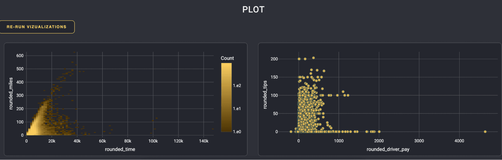
Here’s the resulting visualization for 49 million rows of data. The miles vs time plot ends up being rasterized and the tips vs driver pay is a scatter plot of the aggregated data:

Polars with Plotly Express

In the previous examples, Polars was used for data wrangling in Dash callbacks, and then the resulting Polars dataframes were converted to either a Pandas dataframe, numpy or python list before passing as an argument to the Plotly figure.

As of the latest Plotly python graphing library (v5.16) you can directly pass a Polars DataFrame to Plotly Express.

Wrap Up

We went over what Polars is and why it’s good at handling large data. We also went through two very common, real use cases that come up in Dash applications that can utilize Polars for better performance. I’m sure you’ll find many more ways to implement this library with Dash applications as you dive deeper.

Thinking back to the equity firm that started us down this path, the intended purpose of the Dash application was to leverage the firm’s existing wealth of company data — spanning across the world and all industry sectors, and create an exploratory tool for their team to identify potential companies to invest in.

Before the Professional Services team was involved, this data existed solely in a Redshift database and investment strategists would have to request specific filters/search parameters which the data team would then use to query the dataset to acquire Excel documents with the requested companies.

The Dash application is built utilizing Polars for back-end data handling and is now deployed to Dash Enterprise.

User feedback suggests that the app overall has been a great improvement to their BI workflows, by simplifying this process by providing a platform for their investment team to discover companies, save those companies to lists for future consideration, and share saved companies with colleagues for a more collaborative process — all in one place.

(Image sources: Giphy @gifnews, Reddit)