Chris Parmer

November 9, 2026

Concentration-Time Curves - A Complete Guide

TL;DR

A concentration-time curve plots how much of a drug is in a patient's blood (usually the plasma, the liquid part of the blood) against the time since the dose. After a tablet it rises to a peak and then falls, and pharmacologists draw it twice: on a linear axis to read the peak and the area under the curve, and on a semi-log axis (a logarithmic y axis), where the fall becomes a straight line whose slope gives the half-life.
Concentration-time curves are also known as plasma concentration-time profiles, pharmacokinetic (PK) profiles, and blood level curves. They are line charts with a few conventions of their own, and are the time-course partner of the dose-response curve.
Four numbers come off the curve: Cmax (the peak concentration), Tmax (when it happens), AUC (the area under the curve, the total exposure), and the half-life (the time for the concentration to halve). A green band for the therapeutic range shows whether a dosing schedule keeps the drug where it works.
Drug companies use these curves in phase 1 studies and in the bioequivalence studies that show a generic tablet matches the original, regulators read them in drug submissions, and hospital pharmacists use them to set doses for drugs with a narrow safe range.
You can make a concentration-time curve with Plotly in Python with px.line(..., log_y=True), shade the AUC with fill="tozeroy", and draw the therapeutic range with add_hrect. Code is below.

What is a concentration-time curve?

Concentration-time curves look like this:

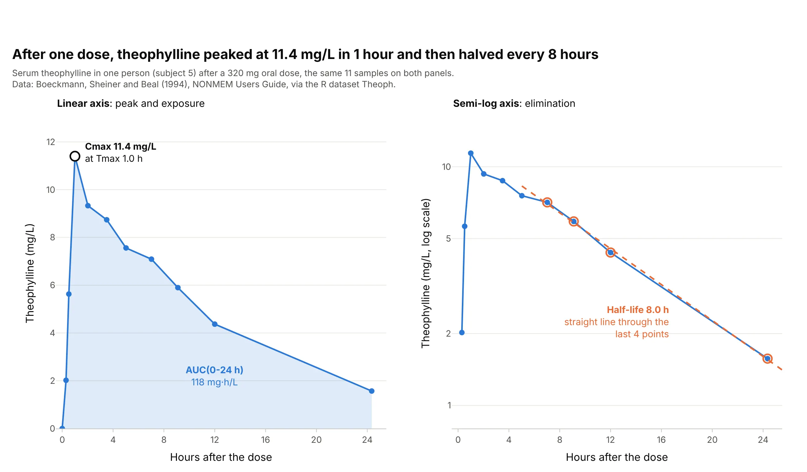
Two panels with the same 11 blood samples of one person after a 320 mg oral dose of theophylline. On the linear left panel, the concentration rises from 0 to a peak of 11.4 mg/L at 1 hour, marked with an open circle as Cmax at Tmax, and falls to 1.6 mg/L at 24 hours, with the area under the curve shaded and labeled AUC(0-24 h) 118 mg·h/L. On the semi-log right panel, the fall after 7 hours is a straight line, and an orange dashed line through the last 4 points is labeled half-life 8.0 h

Data: R dataset Theoph, from a study by Robert Upton reported in Boeckmann, Sheiner, and Beal (1994), NONMEM Users Guide.

How do you read a concentration-time curve? In the example above, notice these things:

The x axis is the time since the dose, in hours, and the y axis is the concentration of theophylline, an asthma drug, in the serum in milligrams per liter (mg/L). Each dot is one blood sample, and the lines join them in a straight line because nothing was measured in between.
The concentration rises while the tablet is absorbed from the gut and falls while the liver clears the drug. Its peak, Cmax, is 11.4 mg/L, measured at Tmax = 1.0 hour after the dose.
The shaded area is the AUC from 0 to 24 hours, 118 mg·h/L. It measures the total exposure to the drug, and it is the number regulators compare when they decide that a generic tablet works like the original.
On the semi-log panel, the same points after 7 hours fall along a straight line, because the body removes a fixed fraction of the drug every hour. The slope of that line gives the half-life: 8.0 hours, so the concentration halves every 8 hours.

It's often used for charts like these:

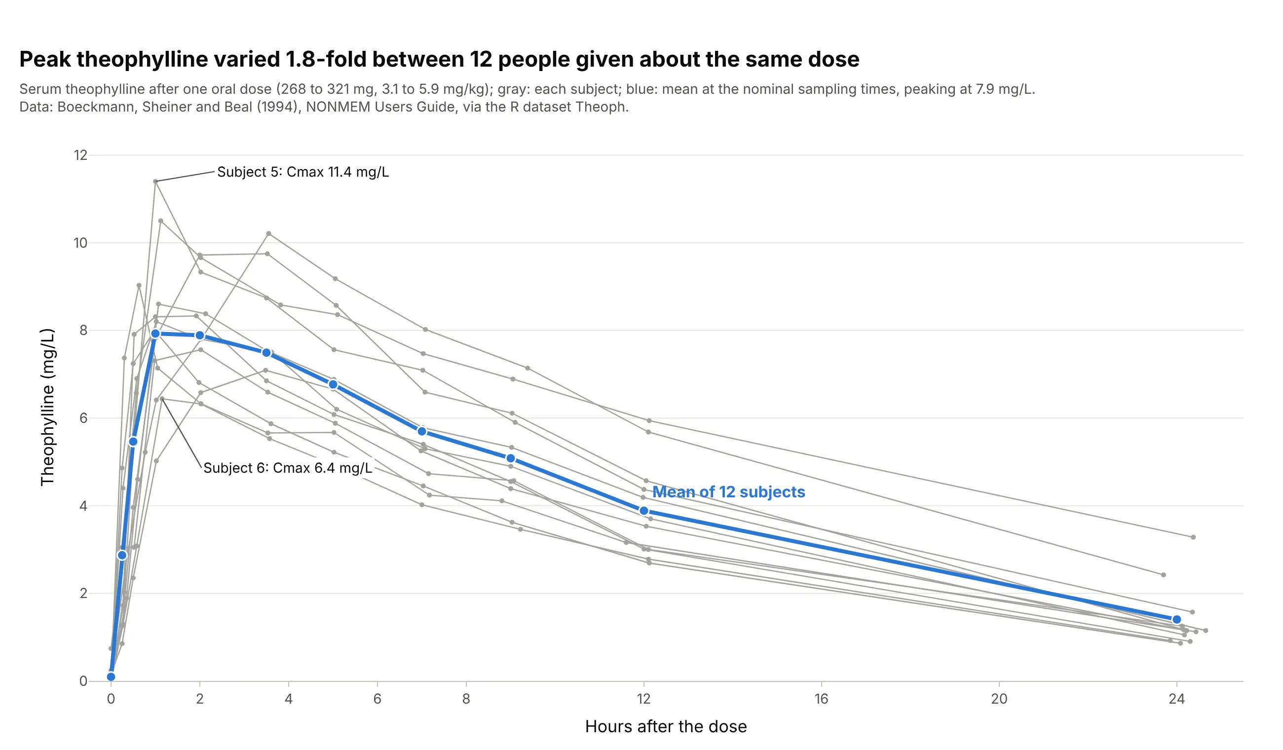
Twelve gray concentration-time curves of theophylline, one per person, rising to peaks between 6.4 mg/L (subject 6) and 11.4 mg/L (subject 5) in the first 4 hours and falling to about 1 mg/L at 24 hours, with the mean of the 12 drawn as a thick blue line that peaks at 7.9 mg/L

Showing how much people differ. A phase 1 study draws every person as a thin line (a spaghetti plot) with the mean on top: in the Theoph study, 12 people given about the same dose reached peaks 1.8-fold apart, from 6.4 to 11.4 mg/L. Data: R dataset Theoph (Boeckmann, Sheiner, and Beal 1994).

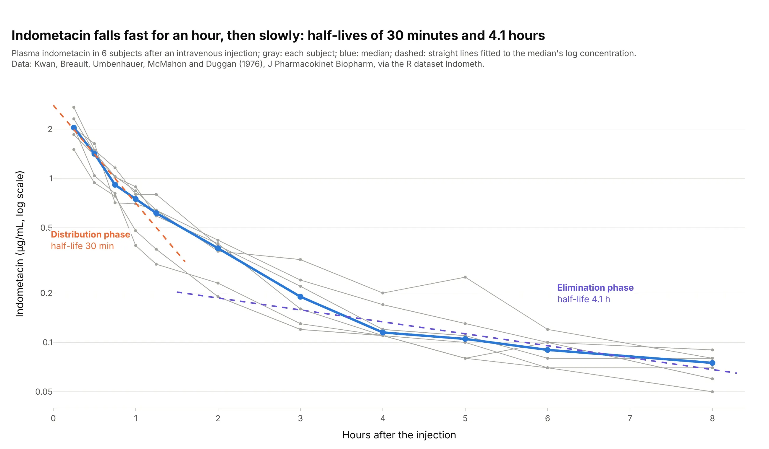
Indometacin concentration after an intravenous injection on a log axis from 0.05 to 2 µg/mL over 8 hours: six gray lines and a blue median fall steeply in the first hour along an orange dashed line labeled distribution phase, half-life 30 min, then slowly along a purple dashed line labeled elimination phase, half-life 4.1 h

Telling how a drug spreads through the body. After an intravenous (IV) injection, indometacin falls along two straight lines on a log axis: a half-life of 30 minutes while the drug spreads from the blood into the tissues, then 4.1 hours while the body eliminates it. Data: R dataset Indometh, from Kwan et al. (1976), Journal of Pharmacokinetics and Biopharmaceutics.

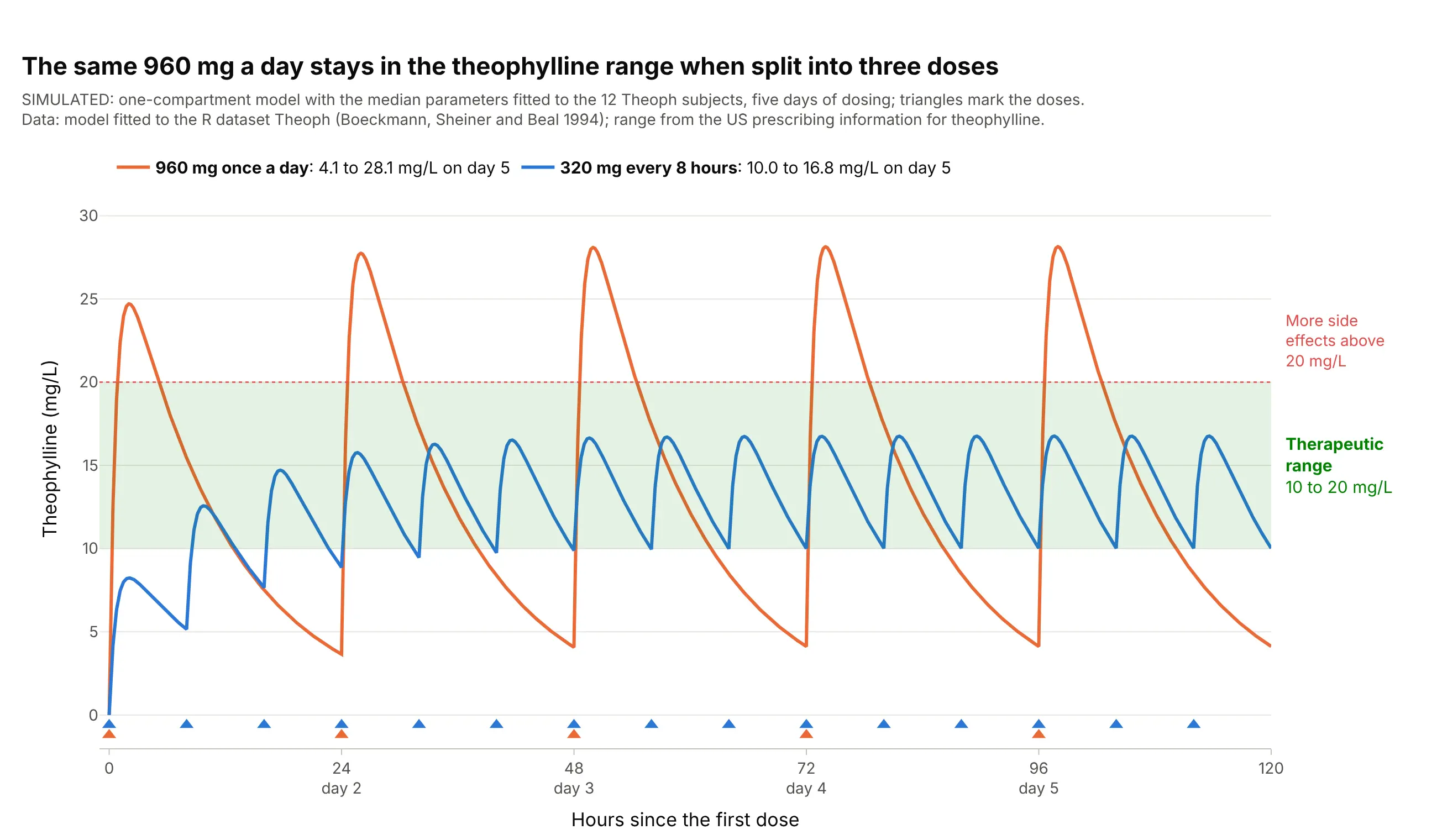
Simulated theophylline concentrations over five days: the orange curve of 960 mg once a day swings from 4.1 to 28.1 mg/L on day 5, far above and below a green band from 10 to 20 mg/L labeled therapeutic range, while the blue curve of 320 mg every 8 hours builds up over two days and then stays between 10.0 and 16.8 mg/L inside the band; triangles at the bottom mark each dose

Choosing a dosing schedule. Dosing decisions are made by drawing the predicted curve against the therapeutic range: in this simulation, the same 960 mg a day stays between 10.0 and 16.8 mg/L when split into three doses, but swings from 4.1 to 28.1 mg/L when given at once. Data: simulated from a one-compartment model fitted to the R dataset Theoph; range from the US prescribing information for theophylline.

A short history

Pharmacokinetics, the study of how the body absorbs, distributes, and eliminates drugs, is usually dated from Torsten Teorell's two 1937 papers on the kinetics of substances given to the body, which earned him the title of father of pharmacokinetics (Paalzow 1995); F. H. Dost named the field in his 1953 book Der Blutspiegel (the blood level), and John Wagner's history of pharmacokinetics (1981) covers the years after. Wagner and Nelson showed in 1963 how to compute the share of a dose absorbed over time from blood level data (Wagner and Nelson 1963), and Yeh and Kwan compared trapezoidal, Lagrange, and spline methods of computing the AUC in 1978 (Yeh and Kwan 1978). The Theoph data in this guide come from the user guide of NONMEM (1994), software for population pharmacokinetic models, and now ship with R. Today the chart is part of the rules: the European Medicines Agency (EMA) asks that "individual plasma concentration/time curves should be presented in linear/linear and log/linear scale" (EMA 2010), and the US Food and Drug Administration (FDA) asks for 12 to 18 samples per subject over at least three half-lives (FDA 2026).

How a concentration-time curve works

A concentration-time curve looks like any line chart over time, but each number on it has a definition that regulators and software agree on. This section explains them one at a time for a reader who doesn't work in pharmacology, using the theophylline data.

Why the curve rises and falls

A drug only works where it reaches, and the blood is where it can be measured. After a tablet, the drug is absorbed from the gut into the blood, so the concentration rises; at the same time the liver and kidneys remove it, so once absorption slows down, the concentration falls. The peak comes when the two rates are equal. An intravenous injection puts the whole dose into the blood at once, so its curve starts at the top and only falls, as in the indometacin chart above.

Most drugs are removed by first-order elimination: the body clears a fixed fraction of what is there every hour, not a fixed amount. That is why the fall is exponential, fast when the concentration is high and slow when it is low, and why it takes the same time to go from 8 to 4 mg/L as from 2 to 1 mg/L.

Cmax and Tmax

Cmax is the highest concentration measured and Tmax is the time it was measured, read straight off the points without fitting anything. Cmax matters for side effects, which often depend on the peak, and Tmax for how fast a drug starts working. Both depend on when the samples were taken: if no sample falls near the real peak, Cmax is underestimated, which is why the EMA asks for frequent samples around the expected Tmax and for the sampling to "avoid Cmax being the first point of a concentration time curve".

AUC: the area under the curve

The AUC adds up the concentration over time, so its unit is concentration times time (mg·h/L), and it measures the total exposure to the drug. Software computes it from the measured points with the trapezoidal rule, one trapezoid per interval between samples:

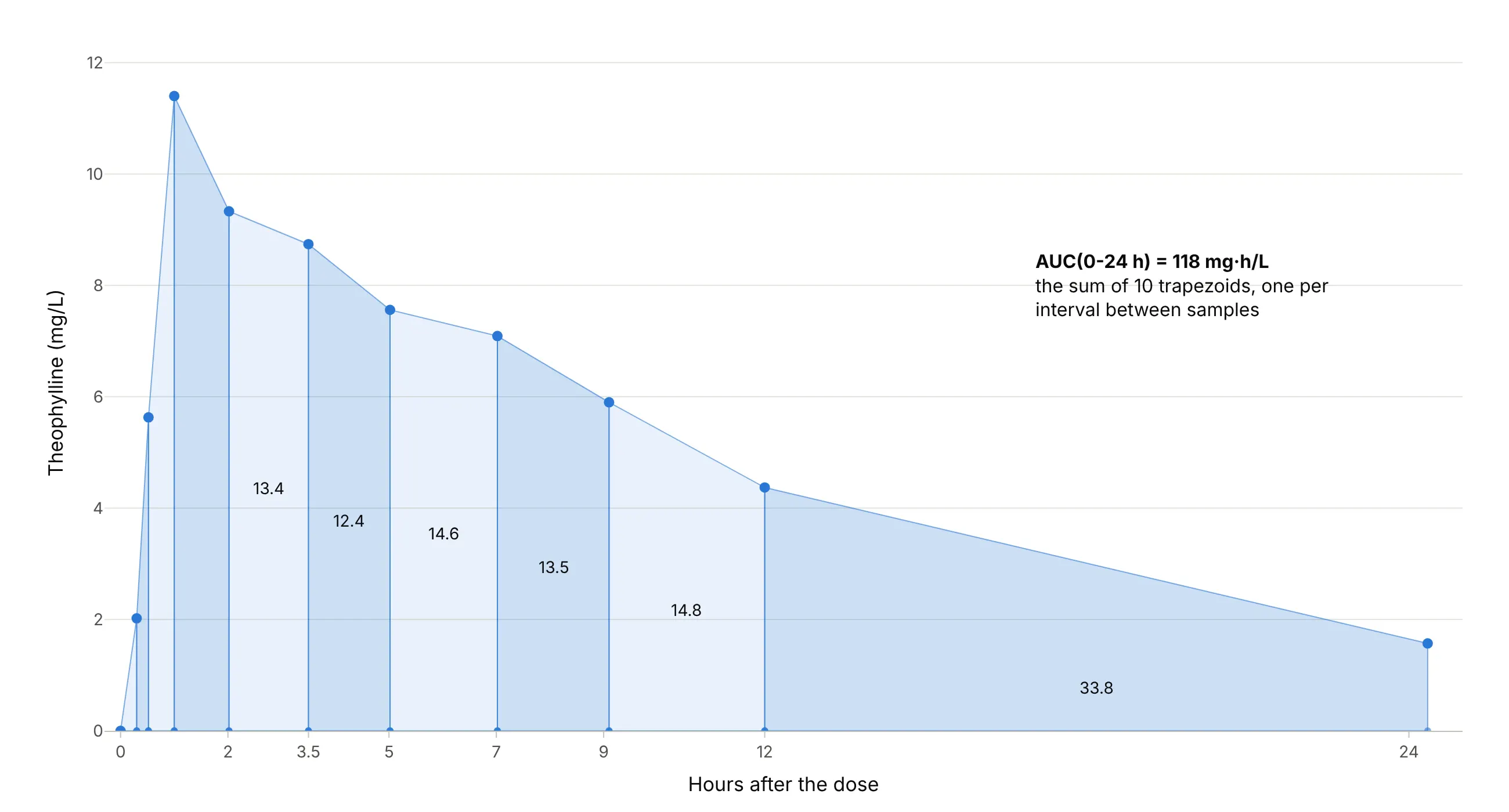
The theophylline curve of subject 5 with the area under it split into 10 trapezoids, one per interval between samples, shaded in alternating light and darker blue, with the areas of the wider ones labeled 13.4, 12.4, 14.6, 13.5, 14.8 and 33.8, and the note AUC(0-24 h) = 118 mg·h/L, the sum of 10 trapezoids

Data: R dataset Theoph, subject 5.

On the falling part the true curve bends below a straight line, so most software uses the linear-up / log-down rule: straight trapezoids while the concentration rises and an exponential shape while it falls. For subject 5 that gives 118 mg·h/L against 121 mg·h/L for straight trapezoids everywhere. The AUC to infinity, AUC(0-inf), adds the area beyond the last sample by extending the terminal slope; regulators want that extrapolated part under 20% of the total, which example 4 below shows.

Half-life and the semi-log axis

On a log y axis, equal ratios get equal distances, so a curve that halves every 8 hours drops by the same distance every 8 hours and becomes a straight line. The slope of that line in natural-log units is the terminal elimination rate constant, λz (lambda z), and the half-life is ln 2 / λz. Software fits the line to the last three or more points after the peak, and the FDA asks for "at least three samples ... during the terminal log-linear phase". In the main example the line through the last 4 points gives λz = 0.087 per hour and a half-life of 8.0 hours, close to the 8.7 hours the theophylline label gives for adults with asthma who don't smoke.

The semi-log axis also shows what a linear axis hides. If the late part of the curve bends instead of running straight, the drug has more than one phase, as for indometacin above, and if the last points flatten out, the assay may be reaching its limit of quantification.

The therapeutic range and steady state

Most drugs are given more than once, and each dose adds a new curve on top of what is left of the last one. The concentration builds up until the amount removed between doses equals the dose, a balance called steady state, reached after about five half-lives (97% of the way, because 1 − 2⁻⁵ = 0.97). For the theophylline model that is about 38 hours, which is why the curves in the dosing chart above level off on day 2.

The therapeutic range (or therapeutic window) is the band between the lowest concentration that works and the concentration where side effects become common. For theophylline the label gives 10 to 20 mg/L and says side effects increase above 20 mg/L, so the chart draws that band in green and asks one question of each schedule: does the curve stay inside it? Drugs with a narrow range, such as theophylline, are often dosed by measuring the concentration in each patient, called therapeutic drug monitoring.

Alternatives to a concentration-time curve

Here's the same Theoph study drawn six ways. Some are better for the question, some worse, some just different:

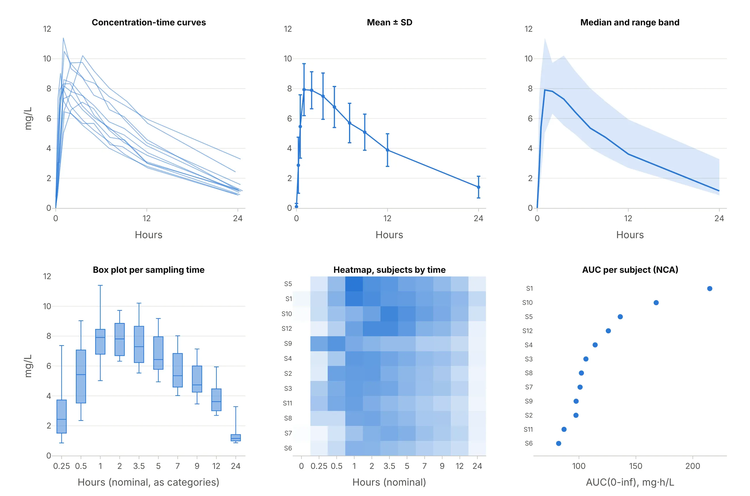
The 12 theophylline profiles drawn six ways: thin concentration-time curves on a true time axis; the mean with standard deviation error bars; the median with a band from the lowest to the highest value at each time; a box plot at each sampling time with the times as equally spaced categories, so 12 to 24 hours looks as short as 0.25 to 0.5; a heatmap of subjects by sampling time in white to blue; and a dot plot of each subject's AUC from about 82 to 215 mg·h/L

Data: R dataset Theoph (Boeckmann, Sheiner, and Beal 1994).

Mean ± standard deviation (SD) error bars (works too, for reports). Study reports and drug labels summarize a group this way, as in example 3 below. It hides individual shapes, and the mean curve's peak (7.9 mg/L) is lower than the average of the individual peaks (8.8 mg/L), because people peak at different times.
Median and range band (works too). A band from the lowest to the highest value at each time, or between percentiles, shows the spread without 12 lines, which is how population model checks are drawn.
Box plot per sampling time (worse). It treats the times as categories, so the 12 hours from 12 to 24 take the same width as the 15 minutes from 0.25 to 0.5, and the shape of the curve is lost.
Heatmap of subjects by time (different). Useful for hundreds of subjects or for spotting a subject whose peak is late, but reading a concentration off a color is hard.
Parameter dot plot (better for comparing many subjects). Once the AUC or Cmax of each subject is computed, one dot per subject ranks them at a glance, and a forest plot of the ratios is how bioequivalence results are reported. It hides the time course that produced the numbers.

The concentration-time curve itself, with the individual lines and a semi-log companion, is the one chart that shows the peak, the exposure, the elimination, and how much people differ, which is why regulators ask for it.

How to make a concentration-time curve

With AI

ChatGPT, Claude Code, GitHub Copilot, Cursor, and other AI tools are excellent at writing Plotly code. Name Plotly in the prompt, and say which axis scales, which parameters, and which reference band you want:

Make plotly concentration-time curves from theoph.csv (columns: Subject, Wt, Dose, Time in hours, conc in mg/L;
12 subjects x 11 samples).

- One thin gray line with markers per subject and the mean at the nominal times in blue, on a linear y axis and
  again on a log y axis side by side.
- For subject 5, shade the AUC to zero, mark Cmax and Tmax, and fit a straight line to ln(conc) over the last
  3 points to get the half-life.
- Draw the therapeutic range of 10 to 20 mg/L as a light green band.
- Check: print Cmax, Tmax, AUC (linear-up / log-down) and the half-life of every subject.

With Plotly Studio

Plotly Studio is a desktop app where you point an AI at a dataset and it builds charts and a Dash app around your questions. Ask for a concentration-time curve the same way:

Show concentration-time curves of conc against Time for each subject, with a toggle between a linear and a log y axis, the mean in bold, a shaded therapeutic range from 10 to 20 mg/L, and a table of each subject's Cmax, Tmax, AUC and half-life.

Make a concentration-time curve in Python or JavaScript

This is the code AI tools write under the hood. You can make a concentration-time curve with Plotly Express from a long table of subject, time, and concentration: px.line with line_group draws one line per subject, log_y=True gives the semi-log version, fill="tozeroy" shades the AUC, and add_hrect draws the therapeutic range.

import numpy as np
import pandas as pd
import plotly.express as px

df = pd.read_csv("theoph.csv")  # Subject, Wt, Dose, Time (h), conc (mg/L): 12 subjects x 11 samples

# Spaghetti plot: one line per subject, on a linear and a log y axis
fig = px.line(df, x="Time", y="conc", line_group="Subject", markers=True)
fig.update_traces(line_color="#a3a29b")
fig.update_layout(template="simple_white", xaxis_title="Hours after the dose", yaxis_title="Theophylline (mg/L)")
fig.show()
fig_log = px.line(df, x="Time", y="conc", line_group="Subject", markers=True, log_y=True)
fig_log.show()


def nca(t, c):
    """Cmax, Tmax, AUC(0-t) by the linear trapezoidal rule, and the half-life from the last 3 points."""
    i = int(np.argmax(c))
    auc = float(np.sum((c[1:] + c[:-1]) / 2 * np.diff(t)))
    slope = np.polyfit(t[-3:], np.log(c[-3:]), 1)[0]
    return dict(cmax=c[i], tmax=t[i], auc=auc, t_half=np.log(2) / -slope)


one = df[df.Subject == 5]
r = nca(one.Time.to_numpy(), one.conc.to_numpy())
fig = px.line(one, x="Time", y="conc", markers=True)
fig.update_traces(fill="tozeroy")                                   # the AUC, shaded to zero
fig.add_hrect(y0=10, y1=20, fillcolor="green", opacity=0.1, line_width=0)  # therapeutic range
fig.add_annotation(x=r["tmax"], y=r["cmax"], text=f"Cmax {r['cmax']:.1f} mg/L at {r['tmax']:.1f} h")
fig.update_layout(template="simple_white", title=f"AUC {r['auc']:.0f} mg·h/L, half-life {r['t_half']:.1f} h")
fig.show()
print({k: round(float(v), 2) for k, v in r.items()})

For subject 5 it prints a Cmax of 11.4 mg/L at 1.0 hour, an AUC of 121.29 mg·h/L, and a half-life of 8.09 hours. The make_pk.py helper in this guide's source code uses the linear-up / log-down rule and picks the number of terminal points by the best adjusted R², a common choice in non-compartmental analysis (NCA) software, which gives 118 mg·h/L and 8.0 hours here.

In JavaScript, plotly.js draws the same curve from the arrays:

<div id="chart"></div>
<script src="https://cdn.plot.ly/plotly-4.1.1.min.js"></script>
<script>
  // Theophylline in subject 5 of R's Theoph dataset after a 320 mg oral dose
  const hours = [0, 0.3, 0.52, 1, 2.02, 3.5, 5.02, 7.02, 9.1, 12, 24.35];
  const conc = [0, 2.02, 5.63, 11.4, 9.33, 8.74, 7.56, 7.09, 5.9, 4.37, 1.57];  // mg/L

  Plotly.newPlot("chart", [{
    x: hours, y: conc, mode: "lines+markers", fill: "tozeroy", name: "Subject 5",
    line: {color: "#2a78d6"}
  }], {
    width: 900, height: 500,
    xaxis: {title: {text: "Hours after the dose"}},
    yaxis: {title: {text: "Theophylline (mg/L)"}},
    shapes: [{type: "rect", xref: "paper", x0: 0, x1: 1, y0: 10, y1: 20, fillcolor: "green", opacity: 0.1,
              line: {width: 0}, layer: "below"}]  // therapeutic range, 10 to 20 mg/L
  });
</script>

Set yaxis: {type: "log"} for the semi-log version, and leave out the zero at time 0, which a log axis can't show.

Share it

Every Plotly chart has a Share chart button (the cloud icon in its toolbar) that uploads it to Plotly Cloud and gives you a link. Only you can see it until you change its visibility.

For a live app, put the chart in a Dash app and publish it with the Plotly Cloud CLI. Coding agents can run these commands for you:

pip install "dash[cloud]"
plotly user login
plotly app publish

If your data has to stay in your own cloud or data center, publish to Dash Enterprise instead.

Dos and don'ts

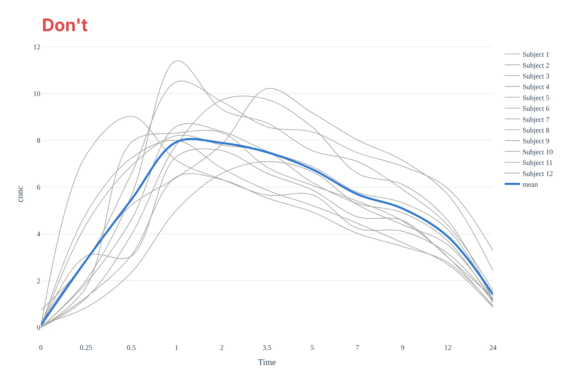
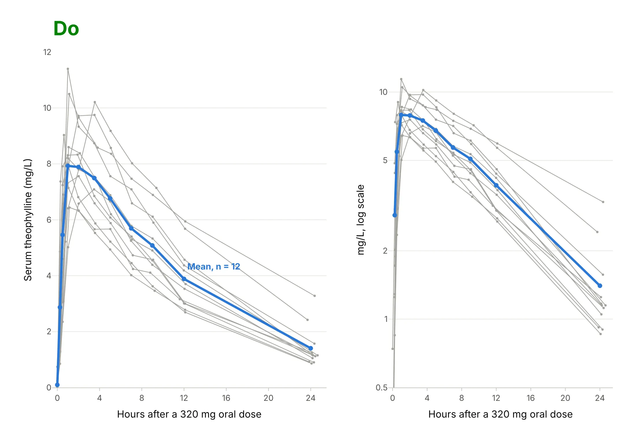
Most mistakes on a concentration-time curve come from treating time as a label instead of a number. Here are the 12 Theoph profiles both ways, in the same gray and blue.

Don't plot the nominal sampling times as equally spaced categories, which makes the 12 hours from 12 to 24 as short as the 15 minutes from 0.25 to 0.5, smooth the lines with splines that invent peaks between samples, leave raw column names without units, or list 12 subjects in a legend:

The 12 theophylline profiles as smooth gray splines and a blue mean against 11 equally spaced time categories from 0 to 24, so the fall from 12 to 24 hours looks as steep as the rise in the first half hour, with axis titles Time and conc, a serif font and a legend of Subject 1 to Subject 12 and mean

Do use a true time axis, join the measured points with straight lines, label the axes with units and the dose, label the mean directly, and add the semi-log panel so the elimination phase can be read:

The same 12 profiles in gray with the blue mean on a true time axis from 0 to 24 hours after a 320 mg oral dose, straight segments between measured points, a y axis titled serum theophylline (mg/L) and the label Mean, n = 12, next to a second panel with a log y axis where the falling parts are straight lines

Checklist

Show the linear and the semi-log view, as the EMA asks for individual curves.
Use the actual sampling times for each subject, and say so if you plot nominal times.
Draw the measured points with straight lines between them, and the fitted model, if any, as a separate smooth line.
Put units on both axes (mg/L or ng/mL, hours or minutes) and state the dose and route.
Draw the therapeutic range or a target as a band, and mark the dose times on repeated-dose charts.
Label simulated curves as simulated.

Don't

Plot zero concentrations on a log axis; they disappear or break the line, so leave them out or mark them as below the limit of quantification.
Estimate the half-life from fewer than three points, or from points that include the peak.
Report an AUC(0-inf) when more than 20% of it is extrapolated.
Average curves of people who peak at different times and present the mean peak as a typical Cmax.

Options to customize

A concentration-time curve in Plotly is a go.Scatter or px.line of concentration against time, so these are the options that matter most. The full lists are in the scatter trace reference, the log axes documentation and the shapes documentation.

px.line(df, x="Time", y="conc", line_group="Subject"): one line per subject from a long table; add color="Subject" only when there are few subjects.
log_y=True or fig.update_yaxes(type="log"): the semi-log axis; set range in log10 units, for example range=[-1, 1.3] for 0.1 to 20 mg/L.
fill="tozeroy": shades the area under the curve; use a second trace for the extrapolated tail.
fig.add_hrect(y0=10, y1=20): the therapeutic range as a band; add_hline for a single target or toxic level.
add_vrect and add_vline: an infusion period or dose times; or a marker trace with symbol="triangle-up" along the bottom.
mode="lines+markers": shows that the line joins measurements; keep line_shape="linear", not "spline".
error_y=dict(type="data", array=sd): mean ± SD at the nominal times.
make_subplots(rows=1, cols=2) or facet_col: linear and semi-log side by side, or one panel per subject.
hovertemplate: subject, time, and concentration with units on hover.
go.Scattergl with all subjects in one trace separated by None: thousands of profiles, as in a population simulation.

More concentration-time curve examples

Six more concentration-time curves built from real public data, each with its source, the technique that makes it work, and a prompt to rebuild it. Most use datasets that ship with R, which is how pharmacokinetics is taught.

1. Warfarin: the concentration peaks in hours, the effect in days

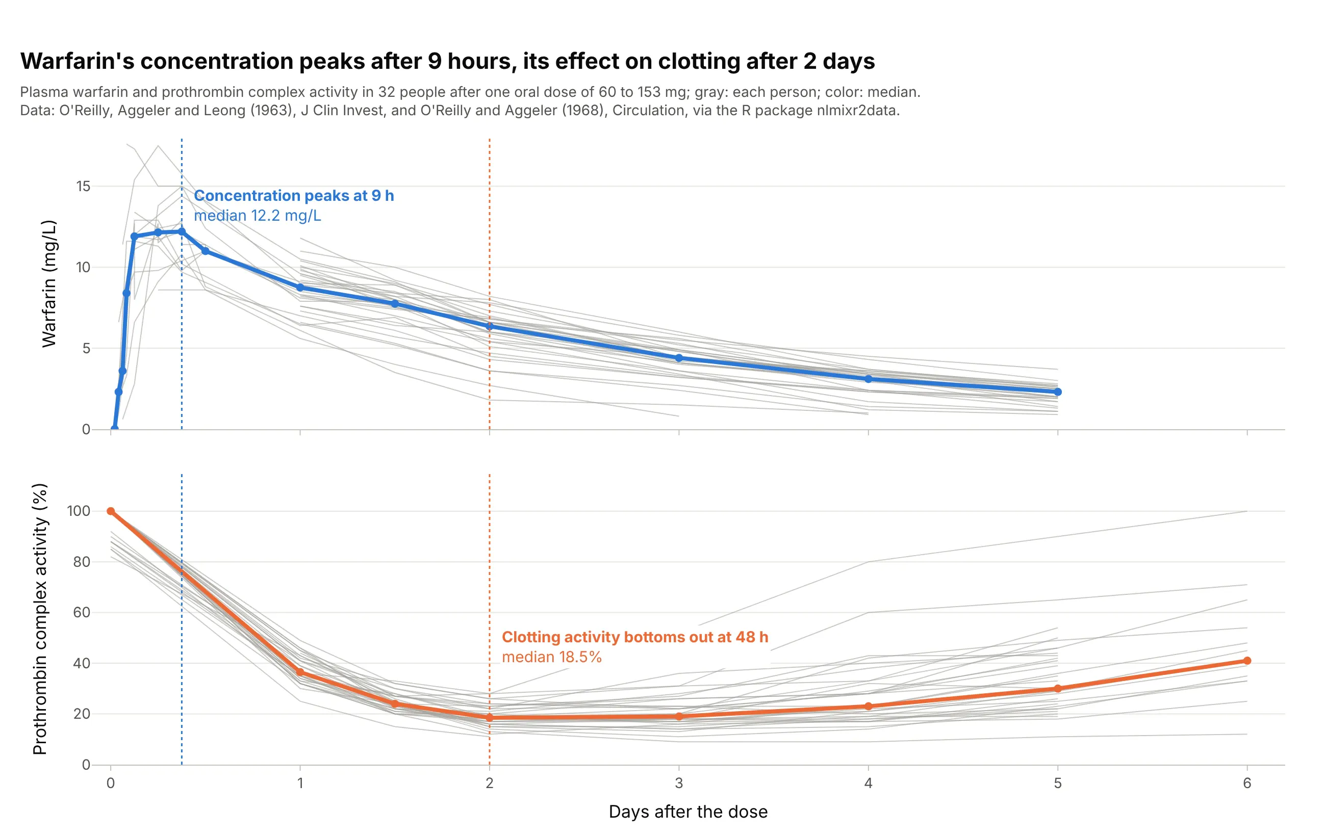
Two panels on one time axis in days for 32 people after one oral dose of warfarin: the top panel's blue median concentration peaks at 12.2 mg/L at 9 hours and falls to 2.3 mg/L at 5 days; the bottom panel's orange median prothrombin complex activity falls from 100% to its lowest, 18.5%, at 48 hours and recovers to 41% at 6 days, with dotted vertical lines at 9 hours and 2 days

Warfarin, a blood thinner, acts on clotting with a delay. The median concentration peaks 9 hours after the dose, but prothrombin complex activity (PCA), a measure of clotting, bottoms out at 48 hours. Data: O'Reilly, Aggeler, and Leong (1963) and O'Reilly and Aggeler (1968), via the R package nlmixr2data.

Tip: stack the concentration and the effect in two panels with a shared time axis, and draw the peak times as vertical lines across both.

Get the data from the warfarin dataset of the R package nlmixr2data (O'Reilly et al. 1963 and 1968: warfarin
concentration in mg/L and prothrombin complex activity in 32 people after one oral dose) and shape it into a table
(columns: id, time_h, dose_mg, value, measure).

Build two plotly panels with a shared x axis in days: concentration and PCA, a thin gray line per person, the
median at each time in color, and dotted vertical lines at the median concentration peak and the lowest PCA.

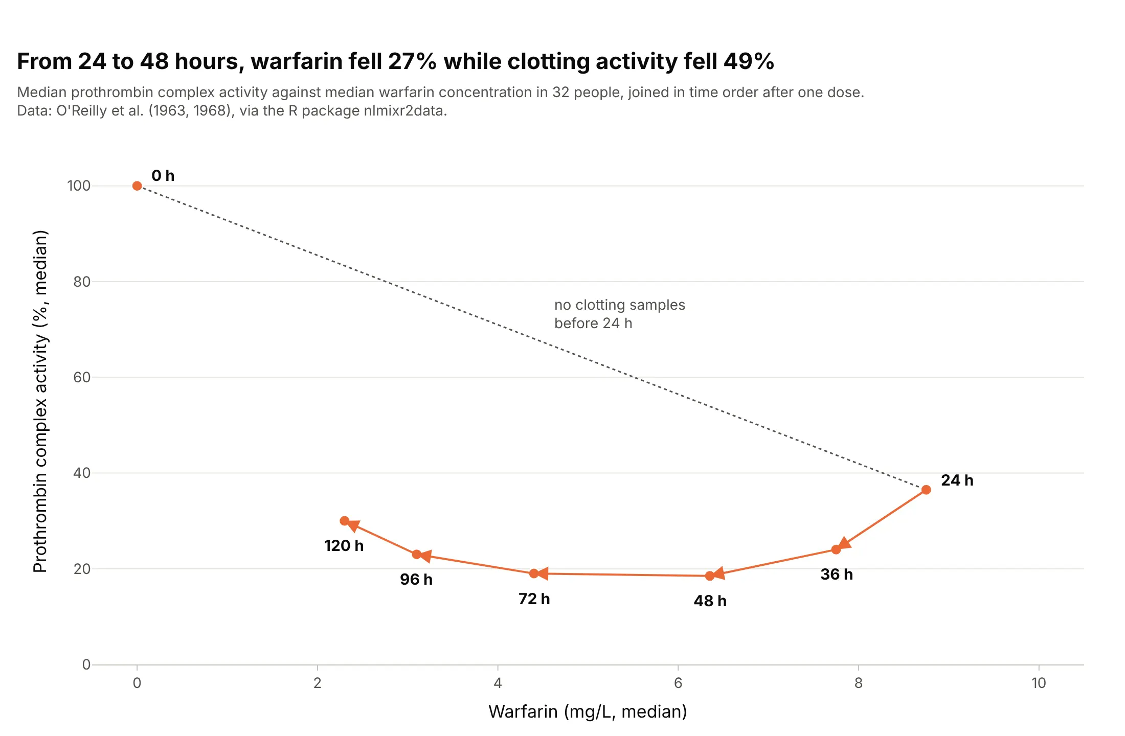
Another way to see it: plotting the effect against the concentration, joined in time order, gives a loop (hysteresis) instead of a single curve. Between 24 and 48 hours, the concentration fell 27% while clotting activity fell 49%:

Median prothrombin complex activity against median warfarin concentration in time order: a dotted line from 100% at 0 mg/L at 0 hours to 36.5% at 8.75 mg/L at 24 hours, labeled no clotting samples before 24 h, then orange arrows to 24% at 36 hours, 18.5% at 48 hours, 19% at 72 hours, 23% at 96 hours and 30% at 2.3 mg/L at 120 hours

2. Remifentanil: half gone in under two minutes

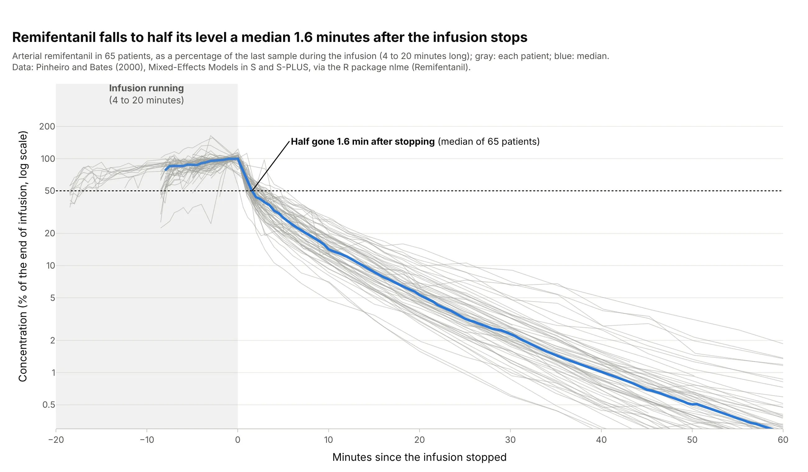
Remifentanil concentration in 65 patients as a percentage of the last sample during an infusion, on a log axis from 0.5% to 200% against minutes since the infusion stopped: gray lines near 100% in a shaded infusion period, then a steep fall through a dotted 50% line, with the blue median reaching 50% 1.6 minutes after stopping and about 1% at 40 minutes

Remifentanil, a strong painkiller given by intravenous infusion, disappears fast once the pump stops. Across 65 patients, the concentration fell to half its end-of-infusion level a median 1.6 minutes after the infusion ended. Data: R package nlme (Remifentanil), from Pinheiro and Bates (2000), Mixed-Effects Models in S and S-PLUS.

Tip: align every patient to the moment the infusion stopped and divide by their level at that moment, so infusions of different lengths and rates can share one axis.

Get the data from the Remifentanil dataset of the R package nlme (Pinheiro and Bates 2000: remifentanil
concentration in ng/ml in 65 patients during and after intravenous infusions, with the infusion rate) and shape it
into a table (columns: id, time_min, conc_ng_ml, rate_ug_min).

Build a plotly chart of minutes since each infusion stopped against concentration as % of the last value during
the infusion, on a log y axis, one gray line per patient, the median in blue, a shaded infusion period and a
dotted line at 50%.

3. The mean ± SD figure from a study report

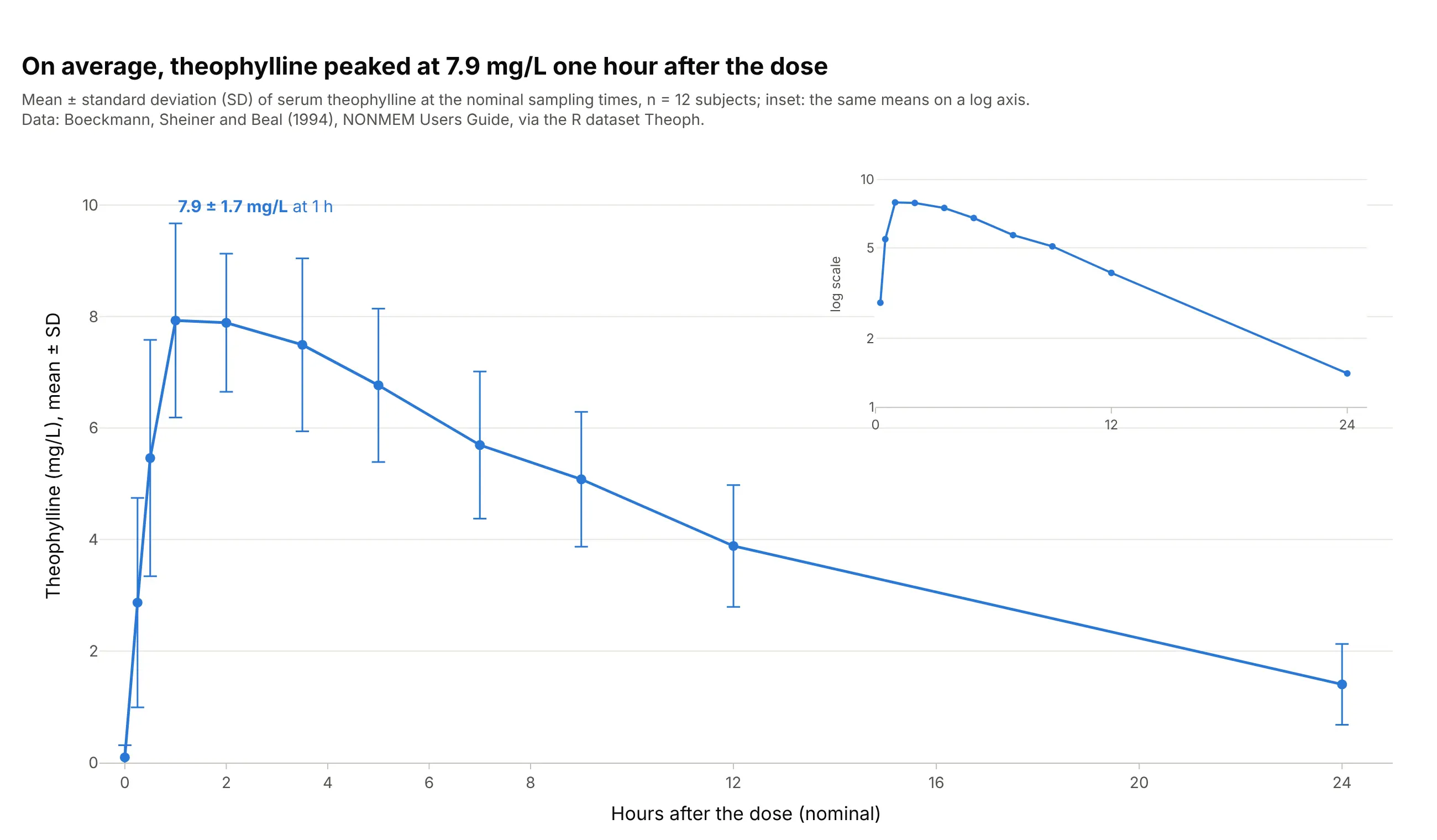
The mean theophylline concentration of 12 subjects at the 11 nominal sampling times with standard deviation error bars on a linear axis, peaking at 7.9 ± 1.7 mg/L at 1 hour and falling to 1.4 mg/L at 24 hours, with an inset in the upper right showing the same means on a log axis where the fall after 2 hours is nearly straight

This is the figure clinical study reports and drug labels use: the mean concentration at each scheduled time with SD error bars, n stated, and the semi-log version as an inset. On average, theophylline peaked at 7.9 ± 1.7 mg/L one hour after the dose. Data: R dataset Theoph (Boeckmann, Sheiner, and Beal 1994).

Tip: put the semi-log inset on its own axes in the empty upper right corner with xaxis2 and yaxis2 domains, so one figure shows both scales.

Get the data from the Theoph dataset in base R (Boeckmann, Sheiner, and Beal 1994: serum theophylline in mg/L of
12 subjects at 11 times over 24 hours after one oral dose) and shape it into a table (columns: subject,
nominal_h, conc_mg_l).

Build a plotly chart of the mean at each nominal time with ± 1 SD error bars on a linear axis, with an inset of
the means on a log y axis in the upper right, and the peak labeled with its mean and SD.

4. When too much of the AUC is extrapolated

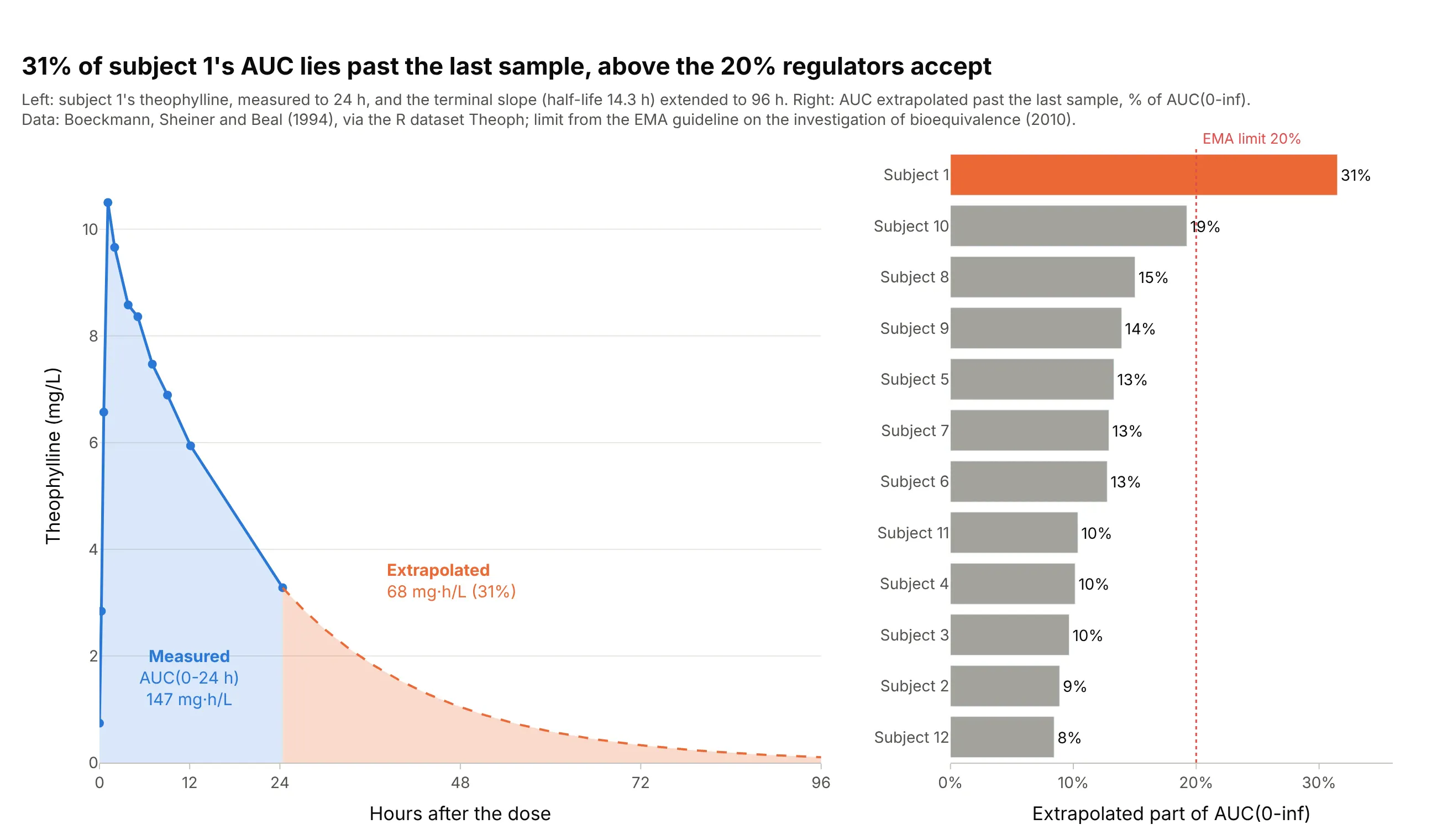
Left: subject 1's theophylline curve with the measured area to 24 hours shaded blue, 147 mg·h/L, and an orange dashed tail extended to 96 hours shaded orange, labeled extrapolated 68 mg·h/L (31%). Right: a sorted bar chart of the extrapolated percentage for all 12 subjects, from 8% to 19% in gray and 31% for subject 1 in orange, with a red dotted line at the EMA limit of 20%

AUC to infinity adds the area past the last sample, estimated from the terminal slope. Subject 1 eliminated theophylline slowly (half-life 14.3 hours), so 31% of their AUC(0-inf) lies past the 24-hour sample, above the 20% the EMA accepts; the other 11 subjects are between 8% and 19%. Data: R dataset Theoph; limit from the EMA bioequivalence guideline.

Tip: shade the extrapolated tail in a second color, so readers see how much of the number is measured.

Get the data from the Theoph dataset in base R (Boeckmann, Sheiner, and Beal 1994: serum theophylline in mg/L of
12 subjects at 11 times over 24 hours after one oral dose) and shape it into a table (columns: subject, time_h,
conc_mg_l).

Compute AUC(0-t) by the linear-up / log-down rule and lambda_z from the last 3 or more points, then build two
plotly panels: subject 1's curve with the measured AUC in blue and the extrapolated tail to 96 h in orange, and a
sorted bar chart of the extrapolated percentage of every subject with a dotted line at 20%.

5. One model fitted to every subject

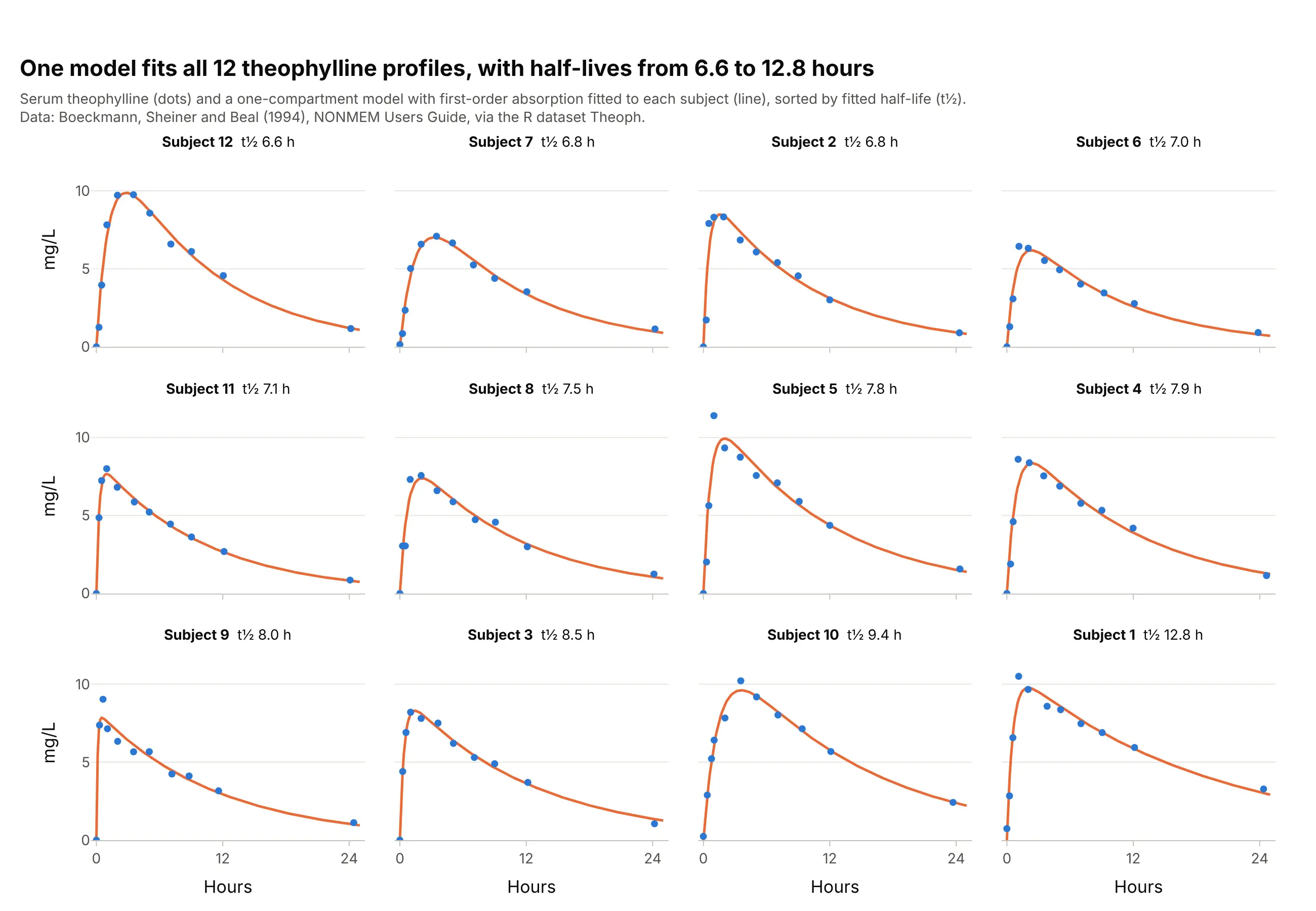
Twelve small panels, one per Theoph subject sorted by fitted half-life from 6.6 hours (subject 12) to 12.8 hours (subject 1), each with the measured concentrations as blue dots and an orange one-compartment model curve rising to a peak in the first 3 hours and falling to about 1 mg/L at 24 hours

Model-based pharmacokinetics fits a compartment model to each person; here a one-compartment model with first-order absorption, the model R's documentation names for the Theoph data (SSfol). One panel per subject shows where the model misses, such as subject 5's sharp early peak, and the fitted half-lives range from 6.6 to 12.8 hours. Data: R dataset Theoph (Boeckmann, Sheiner, and Beal 1994).

Tip: sort the small multiples by a fitted parameter, so the outlier lands at the end instead of somewhere in the middle.

Get the data from the Theoph dataset in base R (Boeckmann, Sheiner, and Beal 1994: serum theophylline in mg/L of
12 subjects at 11 times over 24 hours after one oral dose of about 320 mg) and shape it into a table (columns:
subject, dose_mg, time_h, conc_mg_l).

Fit a one-compartment model with first-order absorption to each subject with scipy, and build a 3 x 4 grid of
plotly panels sorted by fitted half-life, with the measured points, the fitted curve and the half-life in each
panel title.

6. A two-compartment fit on a semi-log axis

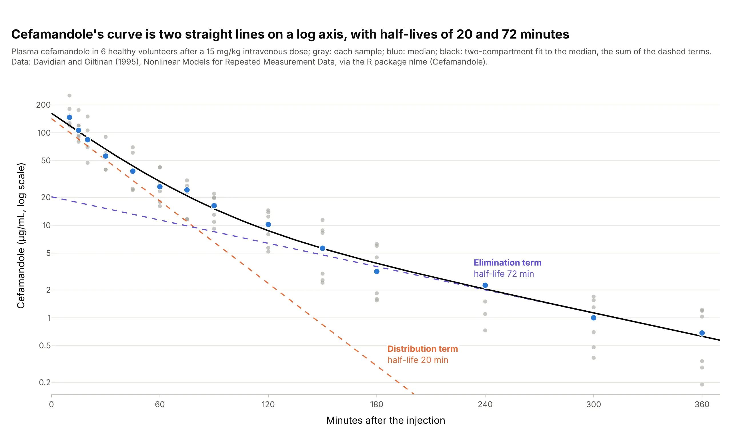
Cefamandole concentrations of 6 people after an intravenous dose on a log axis from 0.2 to 200 µg/mL over 360 minutes: gray samples, blue medians, a black fitted curve that bends, and two dashed straight lines, an orange distribution term with a half-life of 20 minutes and a purple elimination term with a half-life of 72 minutes, whose sum is the black curve

A two-compartment model writes the curve as the sum of two exponentials, and on a semi-log axis each one is a straight line. For the antibiotic cefamandole, the fast term has a half-life of 20 minutes and the slow one 72 minutes. Data: R package nlme (Cefamandole), from Davidian and Giltinan (1995), Nonlinear Models for Repeated Measurement Data.

Tip: draw each term of the fitted model as its own dashed line, so the reader can see which phase dominates when.

Get the data from the Cefamandole dataset of the R package nlme (Davidian and Giltinan 1995: plasma cefamandole in
mcg/ml of 6 healthy volunteers at 14 times over 360 minutes after a 15 mg/kg intravenous dose) and shape it into a
table (columns: subject, time_min, conc).

Fit a biexponential A1 exp(-k1 t) + A2 exp(-k2 t) to the median at each time, and build a plotly chart on a log y
axis with the samples in gray, the medians in blue, the fit in black and each term as a dashed line labeled with
its half-life.