Chris Parmer

November 7, 2026

Dose-Response Curves - A Complete Guide

TL;DR

A dose-response curve plots how strongly something responds (a cell, a plant, a patient) against how much of a drug or chemical it received, with the dose on a logarithmic axis, so the response usually traces an S-shaped (sigmoid) curve between two plateaus.
Dose-response curves are also known as concentration-response curves, dose-response relationships, and exposure-response curves, and when they are fitted with the standard model, four-parameter logistic (4PL) curves. They are similar to scatter plots with a fitted line, and usually carry error bars for the replicates at each dose.
The 4PL, or Hill, model gives four numbers: the bottom and top plateaus, the EC50 (the half-maximal effective concentration, or IC50 for an inhibitor), which measures potency, and the Hill slope, which says how steep the middle is.
Pharmacologists use the curve to rank drug candidates by potency, clinical teams to choose the dose for a phase 3 trial, toxicologists to set safe exposure levels, and labs to read unknown samples off an immunoassay standard curve.
You can make a dose-response curve with Plotly in Python by fitting the 4PL with scipy.optimize.curve_fit and drawing the replicate means with error bars and the fitted curve on a log x axis (type="log"). A short helper function is below.

What is a dose-response curve?

Dose-response curves look like this:

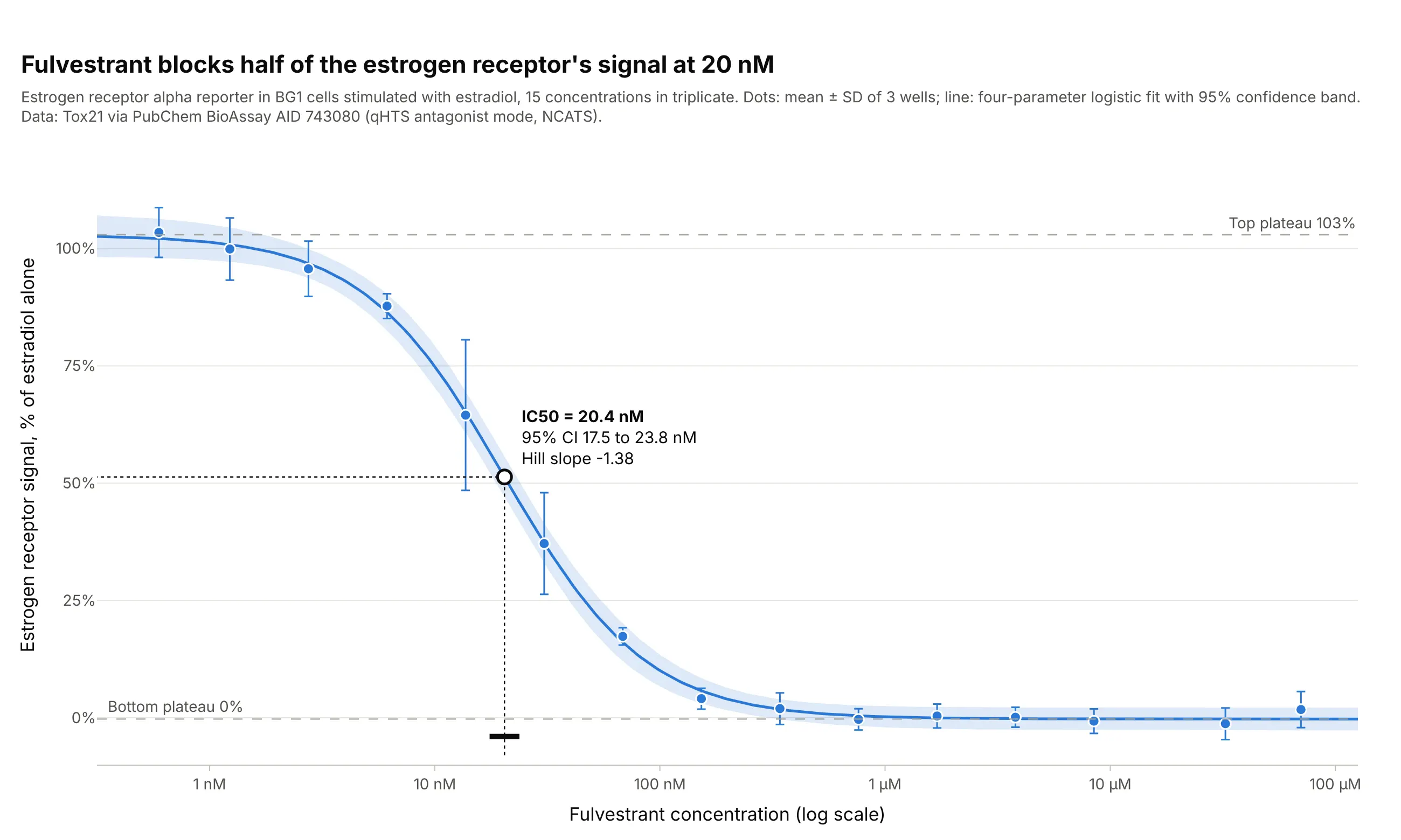
Dose-response curve of fulvestrant in the Tox21 estrogen receptor assay: the signal stays near 100% of estradiol alone up to about 3 nM, falls through a steep S between 6 and 70 nM and flattens near 0% above 300 nM, with blue means and standard deviation error bars of 3 wells, a fitted four-parameter logistic curve with a light blue 95% band, dashed plateaus at 103% and 0%, and an open circle at the IC50 of 20.4 nM, 95% CI 17.5 to 23.8 nM, Hill slope -1.38

Data: Tox21 via PubChem BioAssay AID 743080, the estrogen receptor alpha antagonist screen in BG1 cells run by the US National Center for Advancing Translational Sciences (NCATS).

How do you read a dose-response curve? In the example above, notice these things:

The x axis is the concentration of fulvestrant, a breast cancer drug, on a log scale: each gridline is ten times the one before, from 1 nanomolar (nM) to 100 micromolar (µM). The 15 concentrations are mostly 2.2-fold apart, so they fall almost evenly across the axis.
The y axis is the signal of the estrogen receptor in cells stimulated with estradiol, as a percentage of the signal with estradiol alone. Each dot is the mean of three wells, and its error bar is ± 1 standard deviation (SD) of those wells.
The line is a four-parameter logistic fit. Its top plateau is 103%, its bottom plateau 0%, so fulvestrant blocks the receptor’s signal completely at high concentrations.
The open circle is the IC50, the half-maximal inhibitory concentration: 20.4 nM, with a 95% confidence interval of 17.5 to 23.8 nM (the black bar on the axis). Half the signal is gone at that concentration, and a drug with a lower IC50 is more potent.
The Hill slope of -1.38 says how steep the fall is. It is negative because the curve falls; at a slope of 1, the response goes from 10% to 90% of its range over an 81-fold range of doses, and at 1.38 it takes about 24-fold.

It’s often used for charts like these:

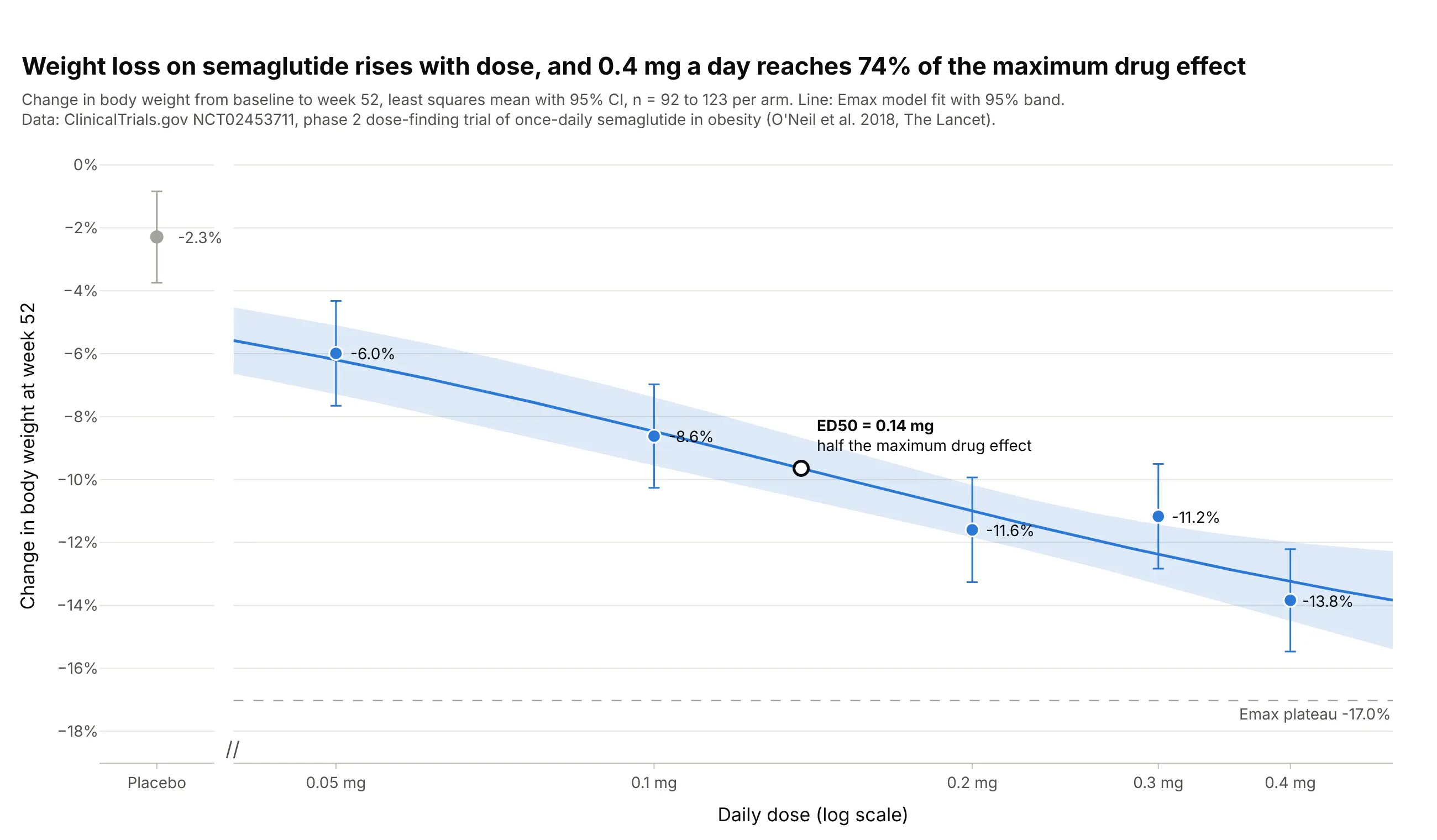
Clinical dose-response curve of weight loss at week 52 for placebo and five daily doses of semaglutide: placebo at -2.3% in its own panel, then -6.0% at 0.05 mg, -8.6% at 0.1 mg, -11.6% at 0.2 mg, -11.2% at 0.3 mg and -13.8% at 0.4 mg with 95% confidence intervals, an Emax curve with its band flattening toward a dashed plateau at -17.0%, and the ED50 of 0.14 mg marked

Choosing the dose in a clinical trial. In a phase 2 trial of daily semaglutide, an Emax model puts half the maximum drug effect at 0.14 mg and 0.4 mg at 74% of it, which is the kind of curve dose-finding studies use to pick the dose for phase 3. Data: ClinicalTrials.gov NCT02453711, O’Neil et al. (2018), The Lancet.

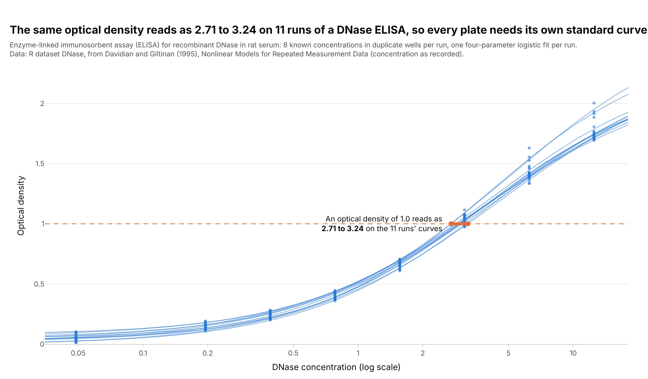
Eleven thin blue four-parameter logistic curves of optical density against DNase concentration on a log axis, one per run of an ELISA, rising from about 0.05 to about 1.9, with the measured wells as small dots and an orange dashed line at an optical density of 1.0 that crosses the curves between concentrations of 2.71 and 3.24

Immunoassay standard curves. An enzyme-linked immunosorbent assay (ELISA) reads unknown samples off a 4PL curve of known standards, and in 11 runs of a DNase ELISA the same optical density of 1.0 reads as 2.71 to 3.24, a 20% spread, which is why every plate gets its own standard curve. Data: R dataset DNase, from Davidian and Giltinan (1995), Nonlinear Models for Repeated Measurement Data.

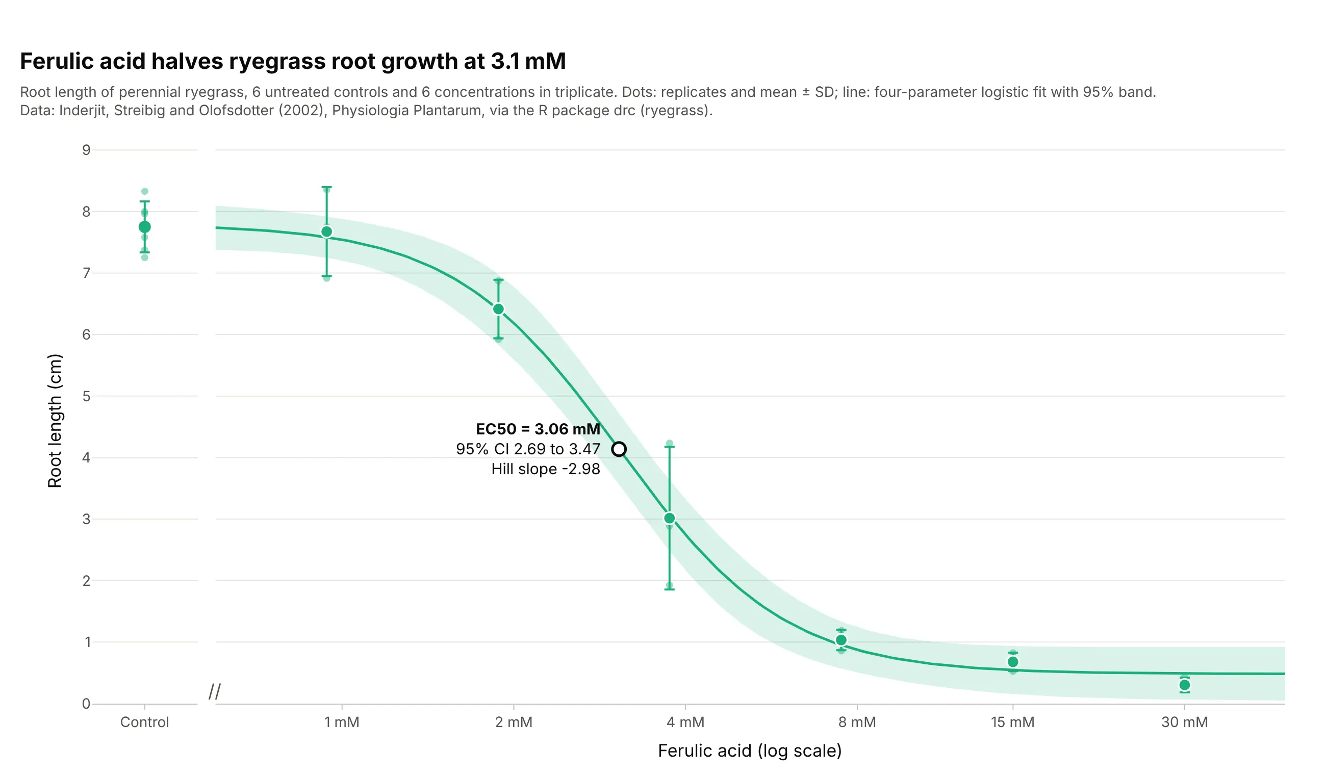
Dose-response curve of ryegrass root length against ferulic acid: 6 untreated controls near 7.7 cm in a narrow panel left of a broken axis, then means with SD error bars at 0.94 to 30 mM falling from 7.7 to 0.3 cm along a green four-parameter logistic curve with a 95% band, and the EC50 marked at 3.06 mM, 95% CI 2.69 to 3.47, Hill slope -2.98

Toxicology and plant science bioassays. The dataset the R package drc starts its documentation with: ferulic acid halves the root growth of ryegrass at 3.06 mM, and the six untreated controls sit in their own panel because a dose of zero has no place on a log axis. Data: Inderjit, Streibig, and Olofsdotter (2002), Physiologia Plantarum, via the R package drc.

A short history

The S-shaped curve comes from physiology. In 1910 A. V. Hill described how hemoglobin takes up oxygen with the equation that now carries his name (Hill 1910), and in 1926 A. J. Clark showed that the response of frog muscle to acetylcholine followed the same form when plotted against the log of the concentration (Clark 1926). J. W. Trevan argued in 1927 that the dose that affects half of a group is a more reliable measure than the smallest dose that has an effect, the idea behind the ED50 and its relatives (Trevan 1927), and Chester Bliss’s probit method (1934) gave a way to fit curves to the share of a group that responds (Bliss 1934). R. P. Stephenson introduced efficacy in 1956, the size of the response a drug can produce, as separate from how strongly it binds (Stephenson 1956), and DeLean, Munson, and Rodbard showed in 1978 how to fit and compare families of four-parameter logistic curves for bioassays, radioligand assays, and physiological dose-response studies (DeLean, Munson, and Rodbard 1978). Today the R package drc (Ritz et al. 2015), GraphPad Prism, and NCATS’s quantitative high-throughput screening (qHTS) pipeline (Inglese et al. 2006) fit these curves by the thousand, and regulators ask for dose-response information in drug submissions: the ICH E4 guideline of the International Council for Harmonisation (ICH), Dose-Response Information to Support Drug Registration (1994), and the US Food and Drug Administration’s exposure-response guidance.

How a dose-response curve works

A dose-response curve looks like a scatter plot with a line through it, but each part follows a convention from pharmacology. This section explains them one at a time, with the fulvestrant data where real data shows the point best and with curves drawn from the equation where it doesn’t.

Why the dose axis is logarithmic

Doses that matter span many orders of magnitude, and the body responds to ratios of dose more than to differences. On a linear axis the fulvestrant data, from 0.6 nM to 70 µM, crush against the left edge; on a log axis each doubling of the dose gets the same room, and the response becomes a symmetric S:

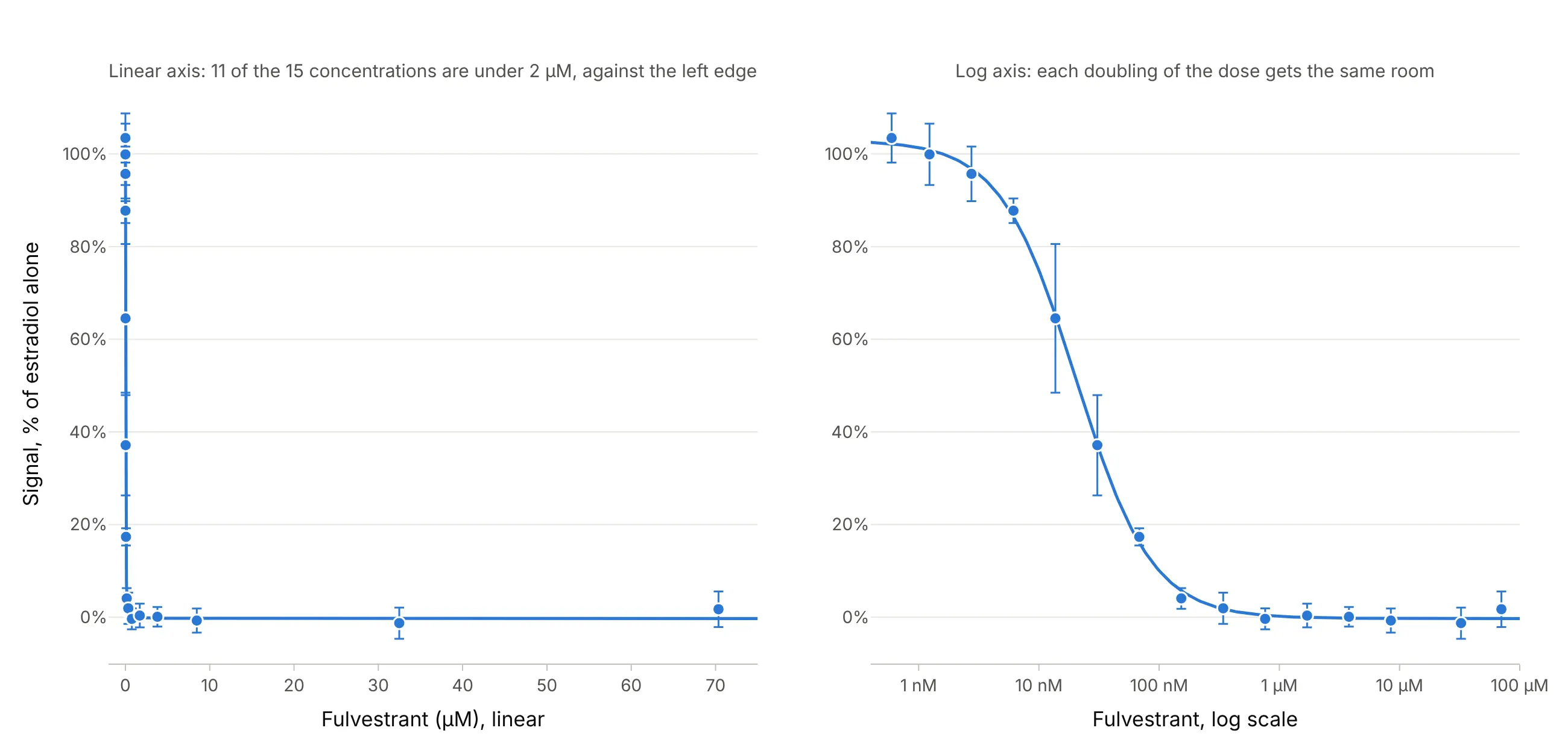
The fulvestrant means plotted twice: on a linear axis from 0 to 70 µM, 11 of the 15 concentrations are under 2 µM and the whole fall from 100% to 0% is a vertical line at the left edge; on a log axis from 1 nM to 100 µM the same points form an even S-shaped curve

Data: Tox21 via PubChem BioAssay AID 743080.

Experiments are designed for this axis too: concentrations are usually a dilution series with a fixed ratio, such as 2-, 3-, or 10-fold steps, so they land evenly on it. GraphPad Prism asks you to enter the log of the concentration, and pharmacology papers often label the axis as the log of the molar concentration, with ticks at -9, -8, and -7 (GraphPad). Labeling the ticks with the concentrations themselves (1 nM, 10 nM) on a log axis shows the same thing and is easier to read.

The four parameters of the 4PL (Hill) equation

The standard model is the four-parameter logistic, also called the Hill equation or, in GraphPad Prism, “log(agonist) vs. response, variable slope”. Each parameter is one feature you can point to on the curve:

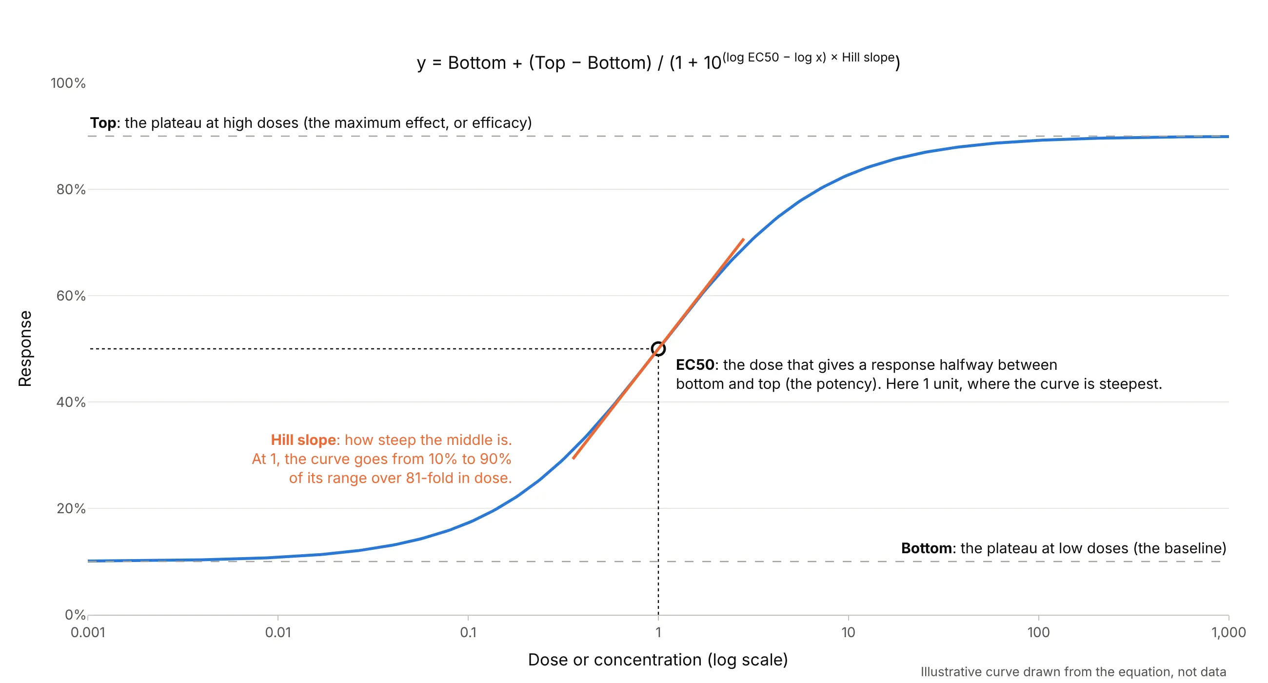
An illustrative S-shaped curve with the 4PL equation above it: a dashed top plateau labeled as the maximum effect or efficacy, a dashed bottom plateau labeled as the baseline, an open circle at the EC50 halfway between them labeled as the potency, and an orange tangent at the middle labeled Hill slope, with the note that at a slope of 1 the curve goes from 10% to 90% over 81-fold in dose

Data: an illustrative curve drawn from the equation, not data.

The EC50 (half-maximal effective concentration) is the dose that gives a response halfway between the bottom and the top, which is not always a response of 50% (GraphPad): the 4-hydroxytamoxifen curve in example 1 below has a top of 118%, so its halfway point is at 62%. For an inhibitor it is called the IC50 (half-maximal inhibitory concentration), for a dose given to a whole animal or person the ED50 (median effective dose), and in the US National Cancer Institute’s NCI-60 cancer cell screen the GI50 (50% growth inhibition). Medicinal chemists often report pEC50 or pIC50, the negative log10 of the molar value, so an IC50 of 20 nM is a pIC50 of 7.7, following the terms of the International Union of Basic and Clinical Pharmacology (IUPHAR) (Neubig et al. 2003).

The Hill slope

The Hill slope, or Hill coefficient, sets how steep the middle of the curve is. At a slope of 1 the response goes from 10% to 90% of its range over an 81-fold range of doses; at 2 it takes 9-fold, and at 0.5 it takes 6,561-fold:

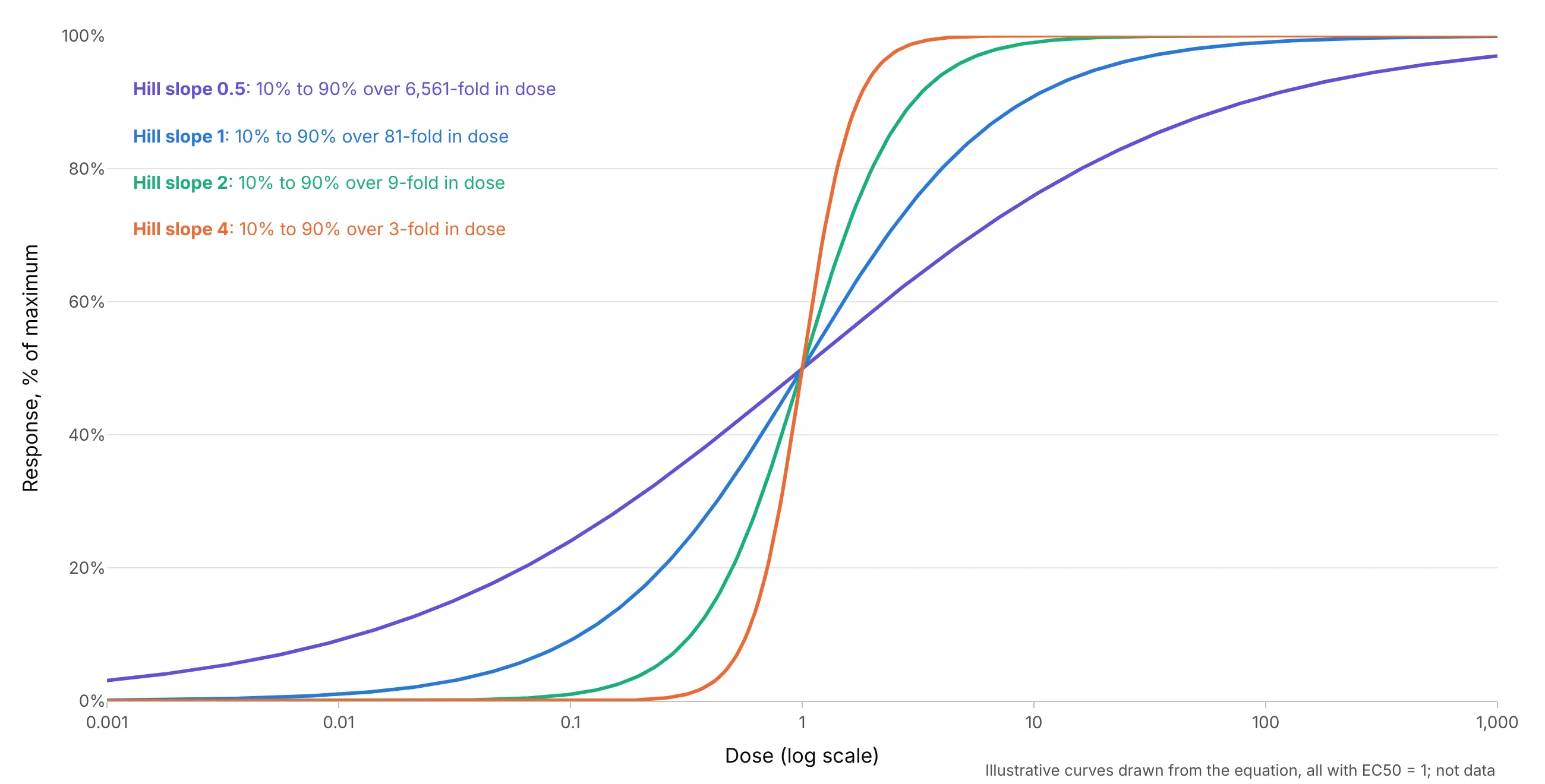
Four illustrative curves with the same EC50 of 1 and Hill slopes of 0.5, 1, 2 and 4, crossing at 50%: the slope 0.5 curve rises slowly over six decades, the slope 4 curve goes from near 0% to near 100% in less than one decade, with labels giving the 10% to 90% span of 6,561-fold, 81-fold, 9-fold and 3-fold

Data: illustrative curves drawn from the equation, all with EC50 = 1; not data.

A slope near 1 is what simple one-to-one binding of a drug to its receptor predicts. Much steeper curves can mean cooperative binding, as in Hill’s hemoglobin, or a threshold effect such as cells dying, and very shallow ones can mean a mix of targets or a compound coming out of solution. Inhibitors get negative slopes in GraphPad’s convention, and drc reports the same curve with the sign flipped, so check which convention a paper uses before comparing slopes.

Potency and efficacy

Two drugs can differ in two ways, and a dose-response curve separates them. Potency is how much drug it takes, read from the EC50: a more potent drug’s curve sits further left. Efficacy is how big the effect can get, read from the top plateau: a partial agonist turns the receptor on, but its curve flattens below a full agonist’s however much you add:

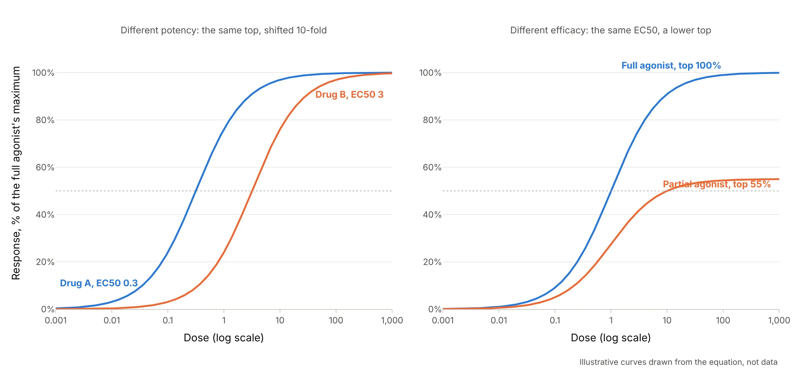
Two panels of illustrative curves: on the left, Drug A with EC50 0.3 and Drug B with EC50 3 have the same top of 100% and are shifted 10-fold apart; on the right, a full agonist reaches 100% while a partial agonist with the same EC50 flattens at 55%

Data: illustrative curves drawn from the equation, not data.

For treatment, efficacy often matters more than potency, since a less potent drug can be given at a higher dose, while no dose of a less efficacious drug makes up the difference. Example 1 below shows potency on real data: four drugs that all block the estrogen receptor completely, at IC50s from 3.4 nM to 12.2 µM.

Agonists and antagonists

An agonist turns a receptor on, so its curve rises with the dose. An antagonist blocks the receptor, so it is tested against an agonist that is already present, and its curve falls. The Tox21 program screens about 10,000 chemicals both ways on the estrogen receptor, which is how these two curves come from the same cells:

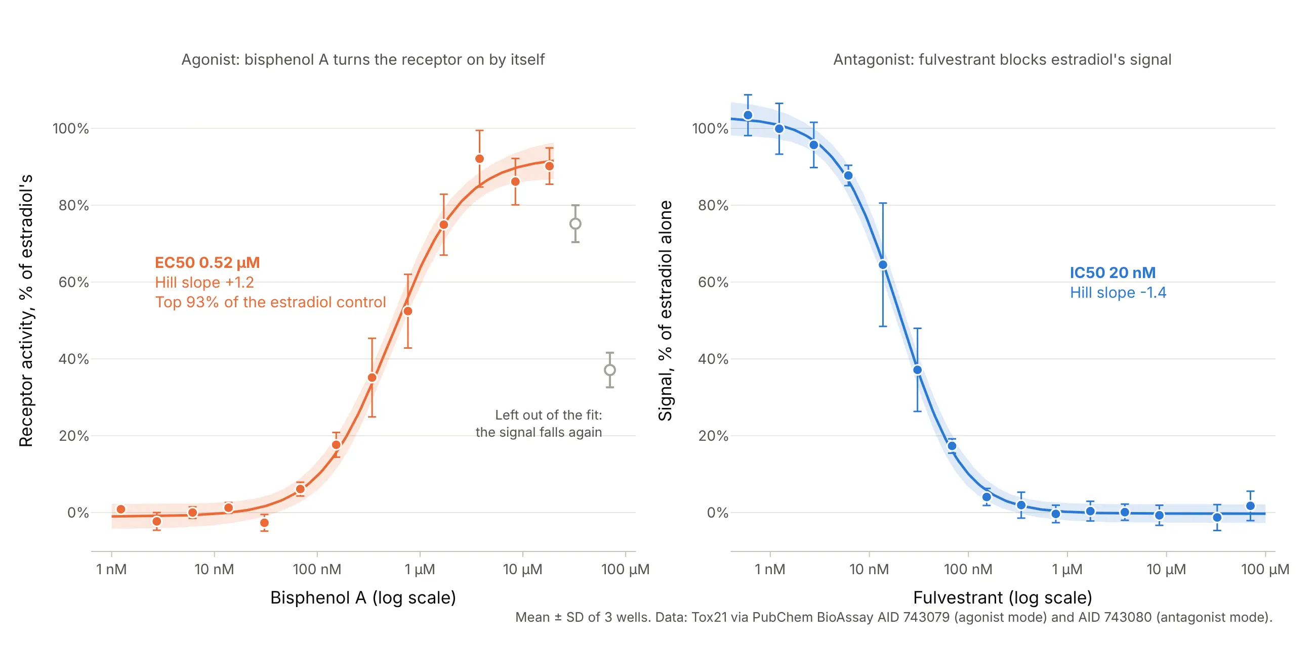
Two panels from the Tox21 BG1 estrogen receptor assays: on the left, bisphenol A in agonist mode rises from 0% to a top of 93% of the estradiol control with an EC50 of 0.52 µM and Hill slope +1.2, with two gray open circles at the highest concentrations left out of the fit because the signal falls again; on the right, fulvestrant in antagonist mode falls from 100% to 0% of estradiol alone with an IC50 of 20 nM and Hill slope -1.4

Data: Tox21 via PubChem BioAssay AID 743079 (agonist mode) and AID 743080 (antagonist mode).

Bisphenol A, a chemical used in some plastics, activates the receptor with an EC50 of 0.52 µM, which is how screening programs flag possible endocrine disruptors. Its signal falls again at the two highest concentrations, so those points are left out of the fit and shown as open circles. This is a common choice when a curve turns down for a reason the model doesn’t describe, such as cells starting to die, and it should be shown on the chart, not done silently.

Error bars and confidence bands

A dose-response chart usually carries two kinds of uncertainty, and they answer different questions. Error bars describe the replicates at each dose, and a confidence band describes the fitted curve:

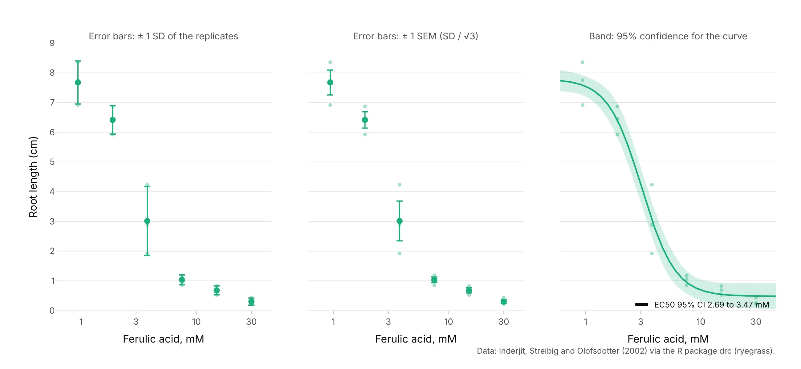
Three panels of the ryegrass data: means with error bars of plus or minus 1 standard deviation of the replicates, the same means with shorter error bars of plus or minus 1 standard error of the mean, and the fitted curve with its 95% confidence band and a black bar at the bottom for the EC50’s 95% confidence interval of 2.69 to 3.47 mM

Data: Inderjit, Streibig, and Olofsdotter (2002), via the R package drc (ryegrass).

The standard deviation (SD) shows how much single wells or plants vary, and the standard error of the mean (SEM), the SD divided by the square root of the number of replicates, shows how precisely the mean is known, so it shrinks as you add replicates. Both are common, so say which one you drew. The confidence band comes from the fit’s covariance matrix (the delta method, which drc uses) and is narrowest near the EC50, where the data pin the curve down. The EC50’s own interval is computed on the log scale, because that is the parameter the fit estimates, which is why it is asymmetric around the EC50 in concentration units. Our error bars guide covers the choice in more detail.

Controls at zero dose

A dose of zero is minus infinity on a log axis, so the untreated controls can’t be plotted there. The convention, which the drc package draws with plot(..., broken = TRUE) and the ryegrass and semaglutide charts above use, is a broken axis: the controls at the left, separated by a break mark, and the doses on the log axis to the right. The fit can still use the controls, because the 4PL approaches its top or bottom plateau as the dose goes to zero.

Alternatives to a dose-response curve

Here’s the same four estrogen receptor antagonists drawn six ways. Some are better for the question, some worse, some just different:

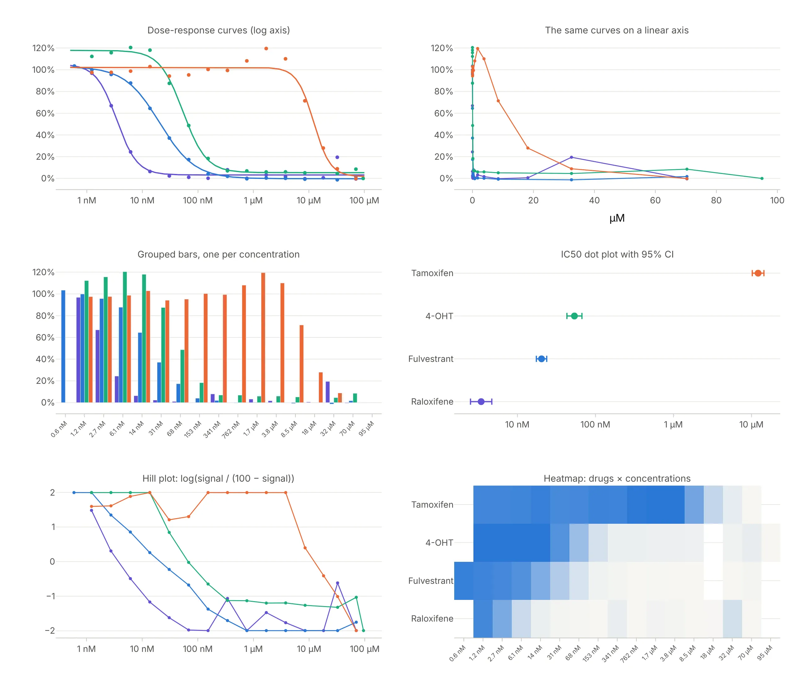
The four antagonists raloxifene, fulvestrant, 4-hydroxytamoxifen and tamoxifen drawn six ways: dose-response curves on a log axis with clear separation, the same curves on a linear axis where three collapse into a vertical line at the left, grouped bars at 17 concentrations, an IC50 dot plot with 95% confidence intervals on a log axis from about 3 nM to 12 µM, a Hill plot of log signal over 100 minus signal, and a heatmap of drugs by concentrations from blue to white

Data: Tox21 via PubChem BioAssay AID 743080.

Line chart or scatter on a linear axis (worse). Three of the four curves collapse into a vertical line at the left, and the difference in potency, the whole point, disappears.
Grouped bar chart (worse). One bar per drug per concentration makes 60 bars that are hard to compare, and the bars treat concentrations as categories, so uneven steps look even.
IC50 dot plot with confidence intervals (better for comparing many compounds). Once the curves are fitted, one dot per compound on a log axis ranks potency at a glance and scales to hundreds of compounds, like a forest plot. It hides the shape, so a partial or bell-shaped curve looks the same as a clean one.
Heatmap of compounds by concentration (different). This is how screening teams look at thousands of compounds at once; the shift of the color edge shows potency, but reading a number off it is hard.
Hill plot (different). Plotting log(response / (100 − response)) against log dose turns a 4PL into a straight line whose slope is the Hill coefficient. It was the way to estimate slopes before computers fitted curves, and it falls apart near the plateaus, as the noisy ends show.

The dose-response curve itself, a scatter plot of the replicates with a fitted line on a log axis, is the one chart that shows potency, efficacy, slope, and the data’s scatter together, which is why papers and regulators expect it.

How to make a dose-response curve

With AI

ChatGPT, Claude Code, GitHub Copilot, Cursor, and other AI tools are excellent at writing Plotly code. Name Plotly in the prompt, and say which model to fit, which error bars to draw, and how to handle the controls:

Make a plotly dose-response curve from fulvestrant.csv (columns: conc_um, signal; 15 concentrations x 3 wells).

- Fit a four-parameter logistic with scipy.optimize.curve_fit:
  y = bottom + (top - bottom) / (1 + 10 ** ((log_ec50 - log10(x)) * hill)).
- Plot the mean of each concentration with +/- 1 SD error bars, the fitted curve and its 95% confidence band
  (delta method from pcov), on a log x axis labeled in nM and µM.
- Mark the IC50 with an open circle and label it with its 95% CI, computed on the log scale.
- Check: print the four parameters and the IC50 with its interval.

With Plotly Studio

Plotly Studio is a desktop app where you point an AI at a dataset and it builds charts and a Dash app around your questions. Ask for a dose-response curve the same way:

Show dose-response curves of signal against concentration on a log axis for each compound, with mean ± SD error bars, a four-parameter logistic fit per compound, the IC50 of each in a table, and a dropdown to pick the compounds.

Make a dose-response curve in Python or JavaScript

This is the code AI tools write under the hood. You can make a dose-response curve with Plotly from a go.Scatter of the means with error_y, a second go.Scatter line of the fitted model, and a log x axis. This helper fits the 4PL with SciPy and returns the figure, and every example in this guide builds on the same idea:

import numpy as np
import pandas as pd
import plotly.graph_objects as go
from scipy.optimize import curve_fit


def logistic4(x, bottom, top, log_ec50, hill):
    """Four-parameter logistic (Hill) curve, in the form GraphPad Prism uses."""
    return bottom + (top - bottom) / (1 + 10 ** ((log_ec50 - np.log10(x)) * hill))


def dose_response(conc, resp, name="", color="#2a78d6"):
    """Means with SD error bars on a log axis and the fitted 4PL curve. Returns the figure and the fit."""
    df = pd.DataFrame({"conc": conc, "resp": resp})
    m = df.groupby("conc").resp.agg(["mean", "std"]).reset_index()
    rising = m["mean"].iloc[-1] > m["mean"].iloc[0]
    p0 = [m["mean"].min(), m["mean"].max(), np.log10(m.conc).median(), 1.0 if rising else -1.0]
    popt, pcov = curve_fit(logistic4, df.conc, df.resp, p0=p0, maxfev=20000)
    xg = np.logspace(np.log10(m.conc.min()) - 0.3, np.log10(m.conc.max()) + 0.3, 300)
    ec50 = 10 ** popt[2]
    fig = go.Figure([
        go.Scatter(x=m.conc, y=m["mean"], error_y=dict(array=m["std"]), mode="markers", name=name,
                   marker=dict(size=10, color=color)),
        go.Scatter(x=xg, y=logistic4(xg, *popt), mode="lines", name="4PL fit", line_color=color),
        go.Scatter(x=[ec50], y=[logistic4(ec50, *popt)], mode="markers+text", name=f"EC50 {ec50:.3g}",
                   text=[f"EC50 {ec50:.3g}"], textposition="middle right", marker=dict(size=12, color="black")),
    ])
    fig.update_xaxes(type="log", title="Concentration (µM, log scale)")
    fig.update_layout(template="simple_white", yaxis_title="Response (%)")
    return fig, popt, pcov


df = pd.read_csv("fulvestrant.csv")  # conc_um, signal: 15 concentrations x 3 wells
fig, popt, pcov = dose_response(df.conc_um, df.signal, name="Fulvestrant")
se = np.sqrt(np.diag(pcov))
print(f"IC50 {1000 * 10 ** popt[2]:.1f} nM, Hill slope {popt[3]:.2f}, log IC50 ± SE {popt[2]:.3f} ± {se[2]:.3f}")
fig.show()

On the fulvestrant data it prints an IC50 of 20.4 nM and a Hill slope of -1.38. For the confidence band, evaluate the curve’s gradient with respect to the four parameters at each x, combine it with pcov (the delta method), and draw the upper and lower bounds as one fill="toself" shape; the R package drc computes the same band for you. One thing to watch: shapes and annotations on a log axis take log10 positions, so put an annotation at x=np.log10(ec50), or draw markers as a trace as above.

In JavaScript, plotly.js draws the same thing from the means and the fitted parameters:

<div id="chart"></div>
<script src="https://cdn.plot.ly/plotly-4.1.1.min.js"></script>
<script>
  // Fulvestrant in the Tox21 estrogen receptor antagonist assay (PubChem AID 743080): mean and SD of 3 wells
  const conc = [0.0005955, 0.001231, 0.002749, 0.006139, 0.01371, 0.03063, 0.06841, 0.1529,
                0.3413, 0.7623, 1.703, 3.794, 8.468, 32.48, 70.35];                       // µM
  const mean = [103.4, 99.9, 95.7, 87.7, 64.5, 37.1, 17.3, 4.0, 1.9, -0.4, 0.4, 0.1, -0.7, -1.3, 1.7];
  const sd = [5.3, 6.6, 5.9, 2.6, 16.0, 10.8, 1.9, 2.2, 3.4, 2.3, 2.6, 2.1, 2.6, 3.4, 3.8];

  // 4PL parameters from the fit in Python: bottom, top plateau, log10 IC50 (µM), Hill slope
  const [bottom, plateau, logIC50, hill] = [-0.29, 102.94, -1.690, -1.381];
  const f = x => bottom + (plateau - bottom) / (1 + Math.pow(10, (logIC50 - Math.log10(x)) * hill));
  const xs = Array.from({length: 300}, (_, i) => Math.pow(10, -3.5 + i * 5.5 / 299));
  const ic50 = Math.pow(10, logIC50);

  Plotly.newPlot("chart", [
    {x: conc, y: mean, mode: "markers", name: "Fulvestrant", error_y: {type: "data", array: sd},
     marker: {size: 10, color: "#2a78d6"}},
    {x: xs, y: xs.map(f), mode: "lines", name: "4PL fit", line: {color: "#2a78d6"}},
    {x: [ic50], y: [f(ic50)], mode: "markers+text", text: [`IC50 ${(ic50 * 1000).toFixed(1)} nM`],
     textposition: "middle right", marker: {size: 12, color: "black"}, showlegend: false}
  ], {
    width: 900, height: 500,
    xaxis: {type: "log", title: {text: "Fulvestrant (µM, log scale)"}},
    yaxis: {title: {text: "Signal, % of estradiol alone"}, ticksuffix: "%"}
  });
</script>

Share it

Every Plotly chart has a Share chart button (the cloud icon in its toolbar) that uploads it to Plotly Cloud and gives you a link. Only you can see it until you change its visibility.

For a live app, put the chart in a Dash app and publish it with the Plotly Cloud CLI. Coding agents can run these commands for you:

pip install "dash[cloud]"
plotly user login
plotly app publish

If your data has to stay in your own cloud or data center, publish to Dash Enterprise instead.

Dos and don’ts

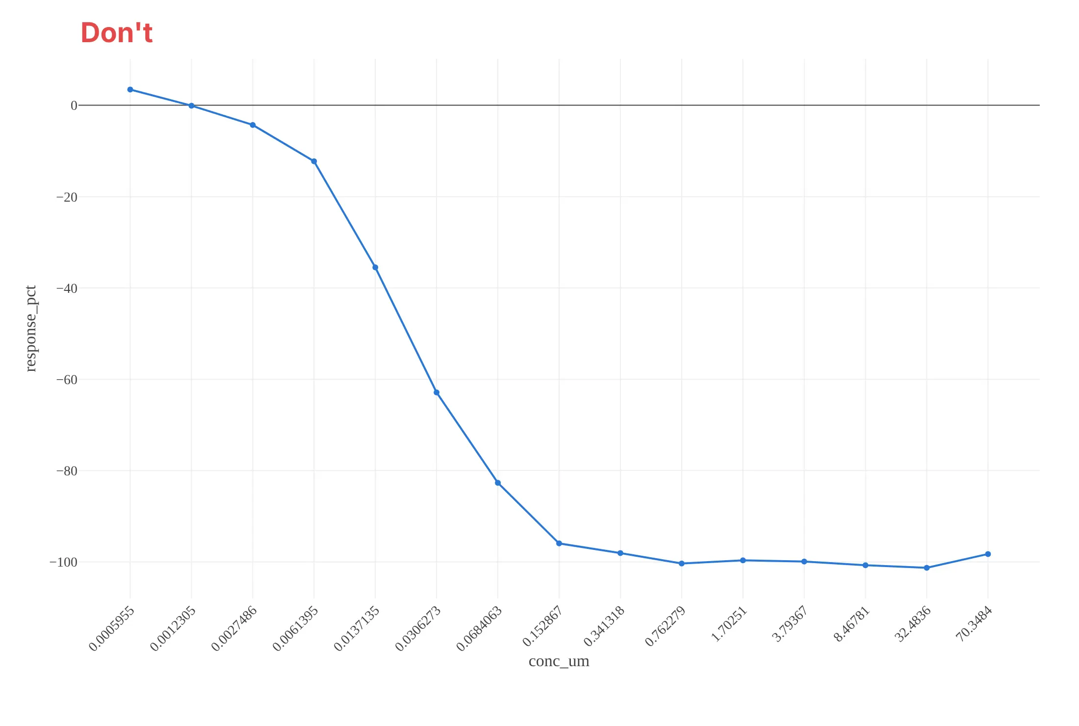
Most of the work in a dose-response chart is putting the doses on the right axis and showing the fit and its uncertainty. Here is the fulvestrant data both ways, in the same blue.

Don’t plot the concentrations as equally spaced categories with raw labels like 0.0005955, which hides that the step from 8.47 to 32.5 µM is 3.8-fold while the others are 2.2-fold, join the means with straight lines instead of fitting a curve, leave out the error bars, or keep raw column names and a serif font:

The fulvestrant means joined by straight blue line segments against 15 equally spaced category labels from 0.0005955 to 70.3484, rotated 45 degrees, with no error bars, the raw axis titles conc_um and response_pct on a scale from 0 to -100, and a serif font

Do use a log concentration axis labeled in nM and µM, show the replicate means with error bars and say what they are, draw the fitted curve with its confidence band, and mark the IC50 with its interval:

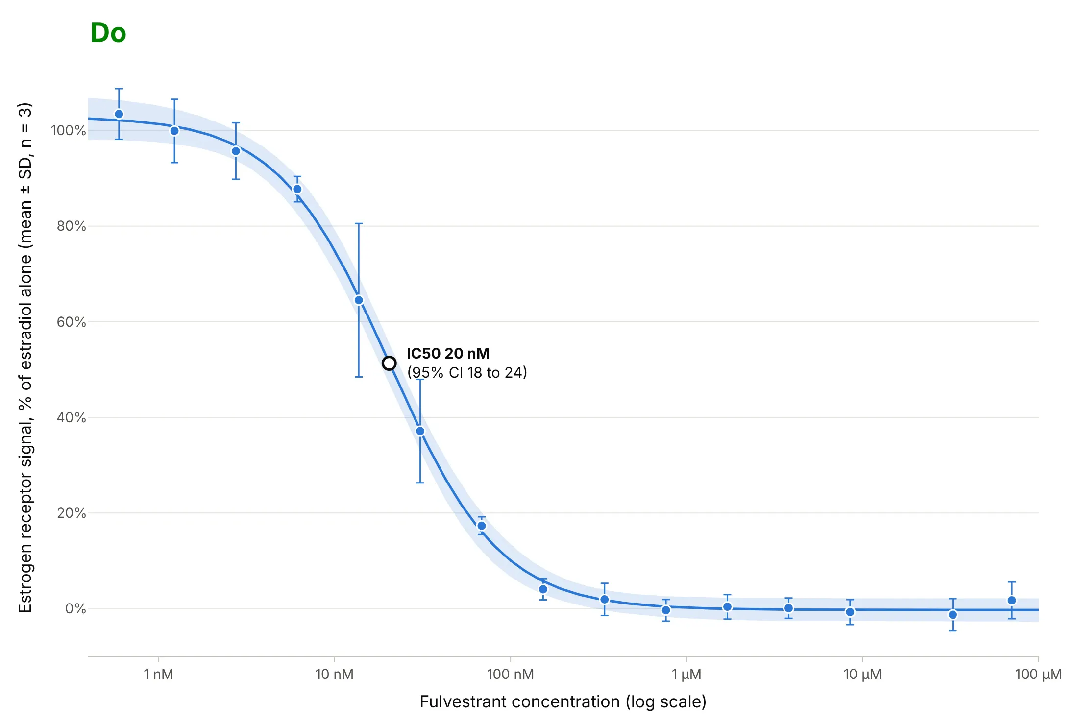
The same fulvestrant data on a log axis from 1 nM to 100 µM, as means with SD error bars along a fitted S-shaped curve with a light blue band, an open circle at the IC50 labeled 20 nM, 95% CI 18 to 24, and a y axis titled estrogen receptor signal, percent of estradiol alone, mean ± SD, n = 3

Checklist

Put the dose on a log axis, and label the ticks with concentrations and units.
Space the doses by a fixed ratio, and cover both plateaus, so the top and bottom are measured rather than guessed.
Show the replicates or their mean with error bars, and say whether the bars are SD, SEM, or a confidence interval.
Report the EC50 or IC50 with a confidence interval computed on the log scale, and the Hill slope.
Plot zero-dose controls in a separate panel on a broken axis.
Compare compounds on one axis in the same assay, and normalize each run to its own controls.

Don’t

Read the EC50 off where the curve crosses 50% when the plateaus aren’t 0% and 100%.
Extrapolate an EC50 beyond the doses you tested; if the curve never reaches a plateau, report “greater than” the top dose.
Drop points that don’t fit without saying so on the chart.
Fit a 4PL to a curve that rises and then falls; use a model for that shape, as in the hormesis example.

Options to customize

A dose-response curve in Plotly is a go.Scatter of the data plus a go.Scatter of the fit on a log axis, so these are the options that matter most. The full lists are in the scatter trace reference, the error bars documentation and the log axes documentation.

fig.update_xaxes(type="log"): the log dose axis; set range in log10 units, for example range=[-3.5, 2] for 0.3 nM to 100 µM.
tickvals and ticktext: label the decades as 1 nM, 10 nM, 100 nM instead of 0.001, 0.01, 0.1.
error_y=dict(type="data", array=sd): error bars from the replicates; add arrayminus for asymmetric intervals such as binomial ones.
go.Scatter(fill="toself"): a confidence band, drawn as one closed shape from the upper bound and the reversed lower bound.
mode="markers" for the data and mode="lines" for the fit, so the data isn’t joined dot to dot.
make_subplots(cols=2, shared_yaxes=True, column_widths=[0.1, 0.9]): a broken axis with the zero-dose controls in their own panel.
add_hline and add_annotation: plateaus, the 50% level, and the EC50 label; on a log axis give annotation positions in log10 units.
hovertemplate: the concentration, mean, and number of replicates on hover.
go.Scattergl: hundreds or thousands of curves on one chart, as in a screening overview.

More dose-response curve examples

Six more dose-response curves built from real public data, each with its source, the technique that makes it work, and a prompt to rebuild it. Five use datasets from the R package drc, which is how most courses teach dose-response analysis.

1. Four estrogen receptor drugs, from 3 nM to 12 µM

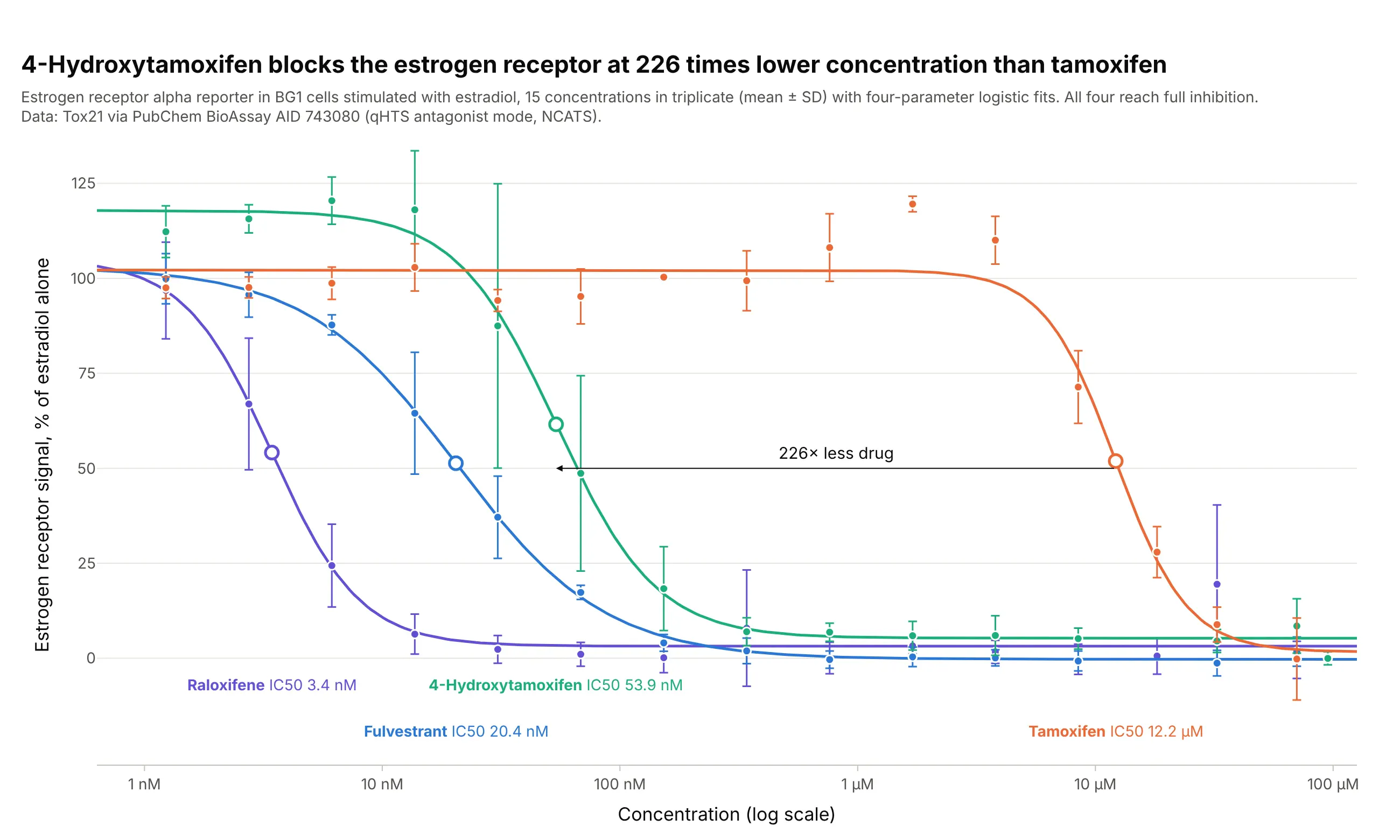
Four dose-response curves from the Tox21 estrogen receptor antagonist assay on one log axis: raloxifene in purple with an IC50 of 3.4 nM, fulvestrant in blue at 20.4 nM, 4-hydroxytamoxifen in green at 53.9 nM with a top near 118%, and tamoxifen in orange at 12.2 µM, all falling to near 0%, with an arrow from tamoxifen’s IC50 to 4-hydroxytamoxifen’s labeled 226 times less drug

All four drugs block the estrogen receptor completely, so they differ in potency, not efficacy. In this assay, 4-hydroxytamoxifen, the form tamoxifen is turned into in the body, needs 226 times less drug than tamoxifen to block half the signal. Data: Tox21 via PubChem BioAssay AID 743080.

Tip: label each curve directly with its IC50, which reads faster than a legend when the curves are side by side.

Get the data from PubChem BioAssay AID 743080 (Tox21 estrogen receptor alpha antagonist screen in BG1 cells,
per-well responses from the PUG REST doseresponse endpoint) for fulvestrant, raloxifene, 4-hydroxytamoxifen and
tamoxifen, and shape it into a table (columns: compound, conc_um, response_pct).

Build plotly dose-response curves of 100 + response_pct on a log axis, mean ± SD per concentration, one 4PL fit
and color per drug, IC50s as open circles, each curve labeled with its name and IC50.

2. Relative potency of two herbicides

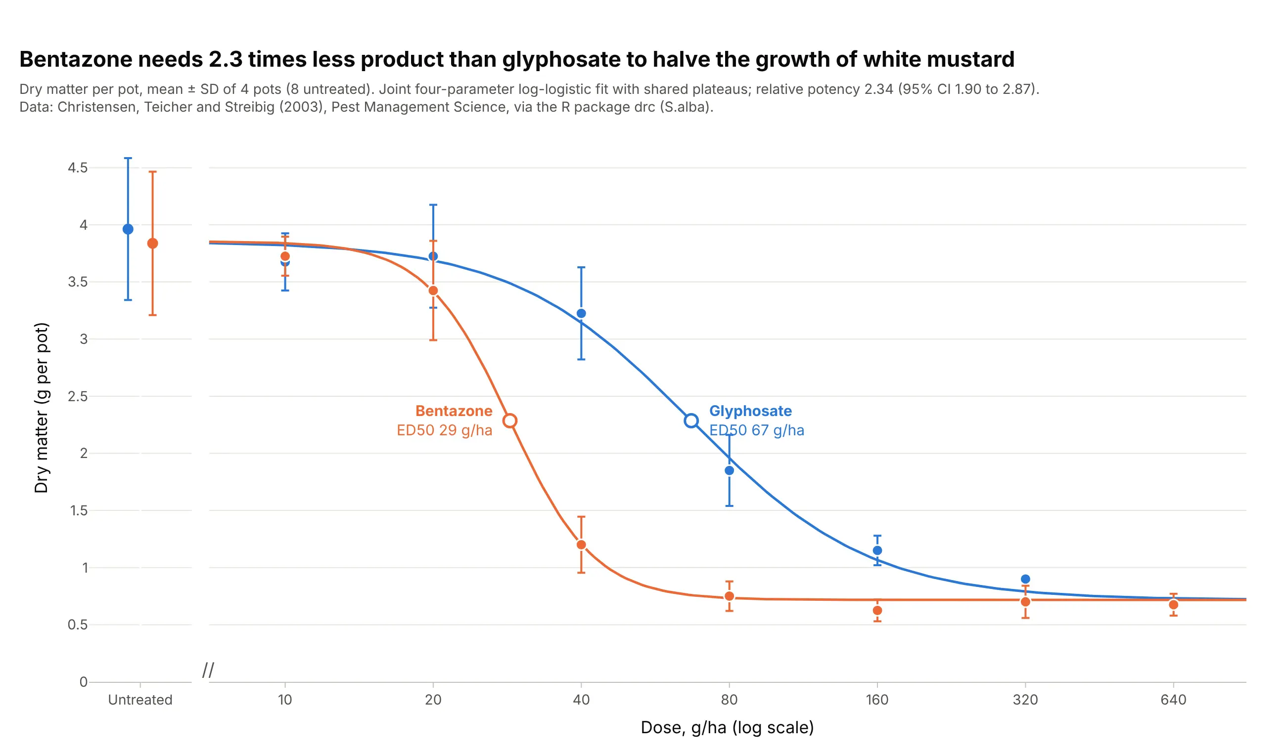
Dose-response curves of white mustard dry matter against glyphosate in blue and bentazone in orange on a log axis from 10 to 640 g/ha, with untreated pots near 3.9 g in a separate panel: both curves share a top of 3.85 g and a bottom of 0.72 g, bentazone’s ED50 is 29 g/ha and glyphosate’s 67 g/ha

When two curves share their plateaus, the ratio of their ED50s is a single relative potency. Bentazone needs 2.34 times less product than glyphosate (95% CI 1.90 to 2.87) to halve the growth of white mustard. Data: Christensen, Teicher, and Streibig (2003), Pest Management Science, via the R package drc (S.alba).

Tip: fit the curves jointly with shared top and bottom, so the potency ratio gets one confidence interval.

Get the data from the R package drc's S.alba dataset (Christensen, Teicher, and Streibig 2003, dry matter of white
mustard in g per pot after glyphosate or bentazone at 0 to 640 g/ha, 4 pots per dose) and shape it into a table
(columns: herbicide, dose_g_ha, dry_matter_g).

Build plotly dose-response curves with a joint 4PL fit that shares bottom and top across herbicides, a broken
axis for the untreated pots, mean ± SD, both ED50s marked and the relative potency with its 95% CI in the subtitle.

3. Water fleas at 24 and 48 hours: a quantal response

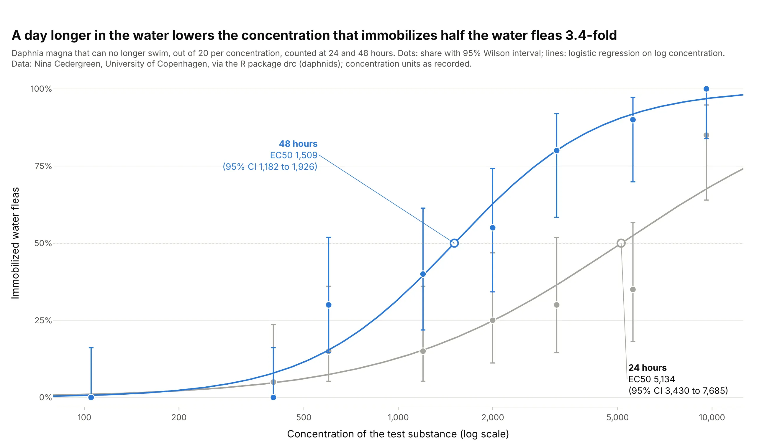
Two dose-response curves of the share of immobilized Daphnia magna out of 20 against concentration on a log axis: the 48 hour curve in blue reaches 100% at the top dose with an EC50 of 1,509, the 24 hour curve in gray is to the right with an EC50 of 5,134, both with 95% Wilson interval error bars

Here the response is the share of 20 water fleas that can no longer swim, a quantal (yes or no) response, fitted with a binomial logistic regression. A day longer in the water lowers the EC50 3.4-fold, from 5,134 to 1,509, which is why the OECD 202 acute immobilisation test reads the animals at both 24 and 48 hours. Data: Nina Cedergreen, University of Copenhagen, via the R package drc (daphnids); test guideline OECD Test No. 202.

Tip: draw binomial confidence intervals (Wilson) as asymmetric error bars with arrayminus, so they stay between 0% and 100%.

Get the data from the R package drc's daphnids dataset (Nina Cedergreen, University of Copenhagen; immobile
Daphnia magna out of 20 at 8 concentrations, counted at 24 h and 48 h) and shape it into a table (columns:
dose, immobile, total, time).

Build a plotly dose-response chart of the share immobilized on a log axis, one binomial logistic regression on
log10 dose per time, Wilson 95% intervals as asymmetric error bars, and each EC50 labeled with its 95% CI.

4. Hormesis: lettuce grows more at low doses

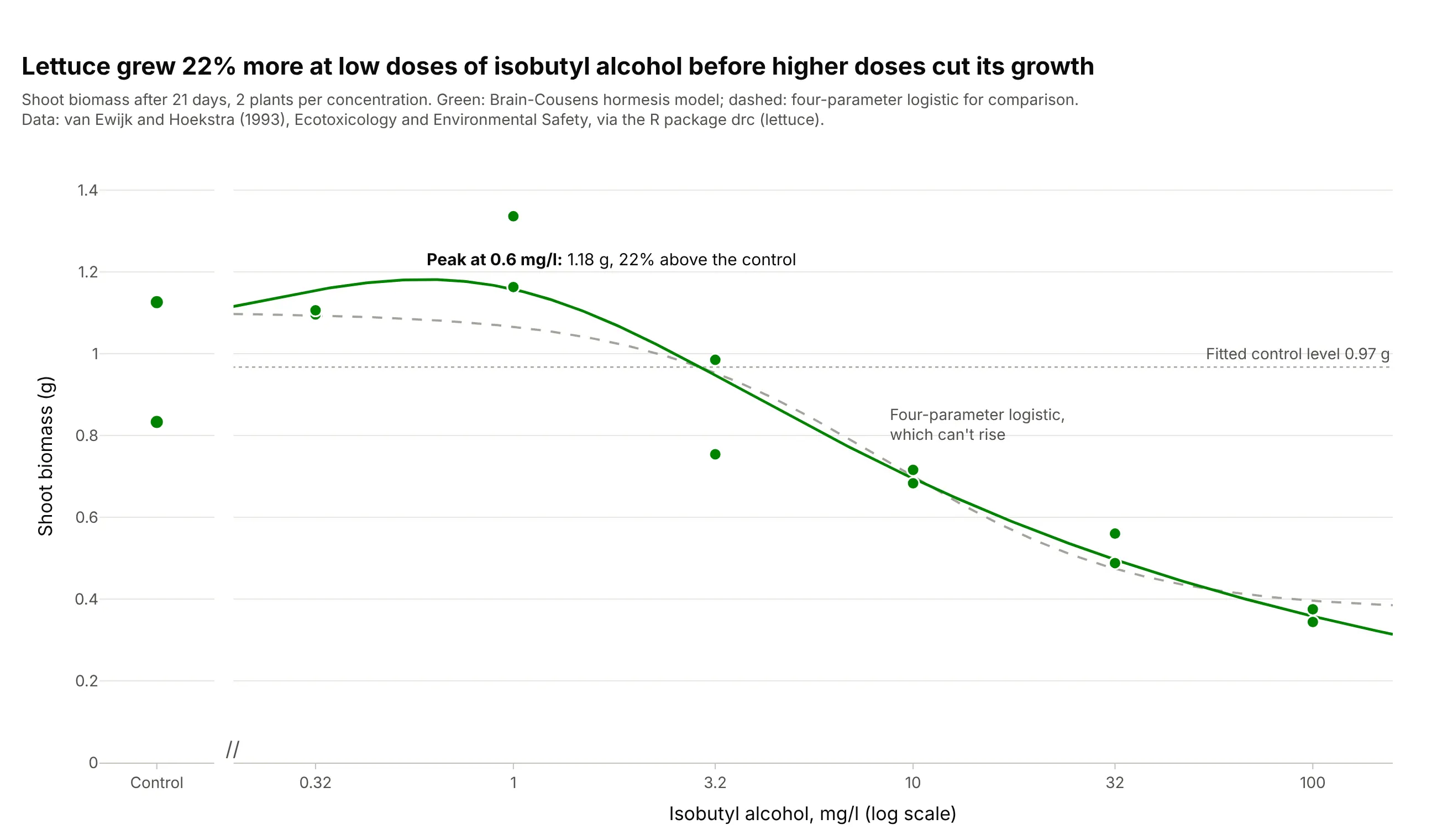
Lettuce shoot biomass against isobutyl alcohol on a log axis with controls in a separate panel: a green Brain-Cousens curve rises from the control level of 0.97 g to a peak of 1.18 g at 0.6 mg/l and then falls to about 0.35 g at 100 mg/l, while a dashed gray four-parameter logistic can only fall, and a dotted line marks the control level

Low doses of isobutyl alcohol raised lettuce growth by up to 22% before higher doses cut it, a pattern called hormesis. A 4PL can only rise or fall, so it misses the peak; the Brain-Cousens model adds a term for the low-dose rise. Data: van Ewijk and Hoekstra (1993), Ecotoxicology and Environmental Safety, via the R package drc (lettuce).

Tip: draw the control level as a reference line, so the rise above it is visible without reading the axis.

Get the data from the R package drc's lettuce dataset (van Ewijk and Hoekstra 1993, shoot biomass of lettuce in
g after 21 days in isobutyl alcohol at 0 to 100 mg/l, 2 plants per concentration) and shape it into a table
(columns: conc_mg_l, biomass_g).

Build a plotly dose-response chart with a Brain-Cousens hormesis fit, a dashed 4PL for comparison, a broken axis
for the controls, a dotted line at the fitted control level and the peak labeled.

5. The baroreflex: an asymmetric curve on a linear axis

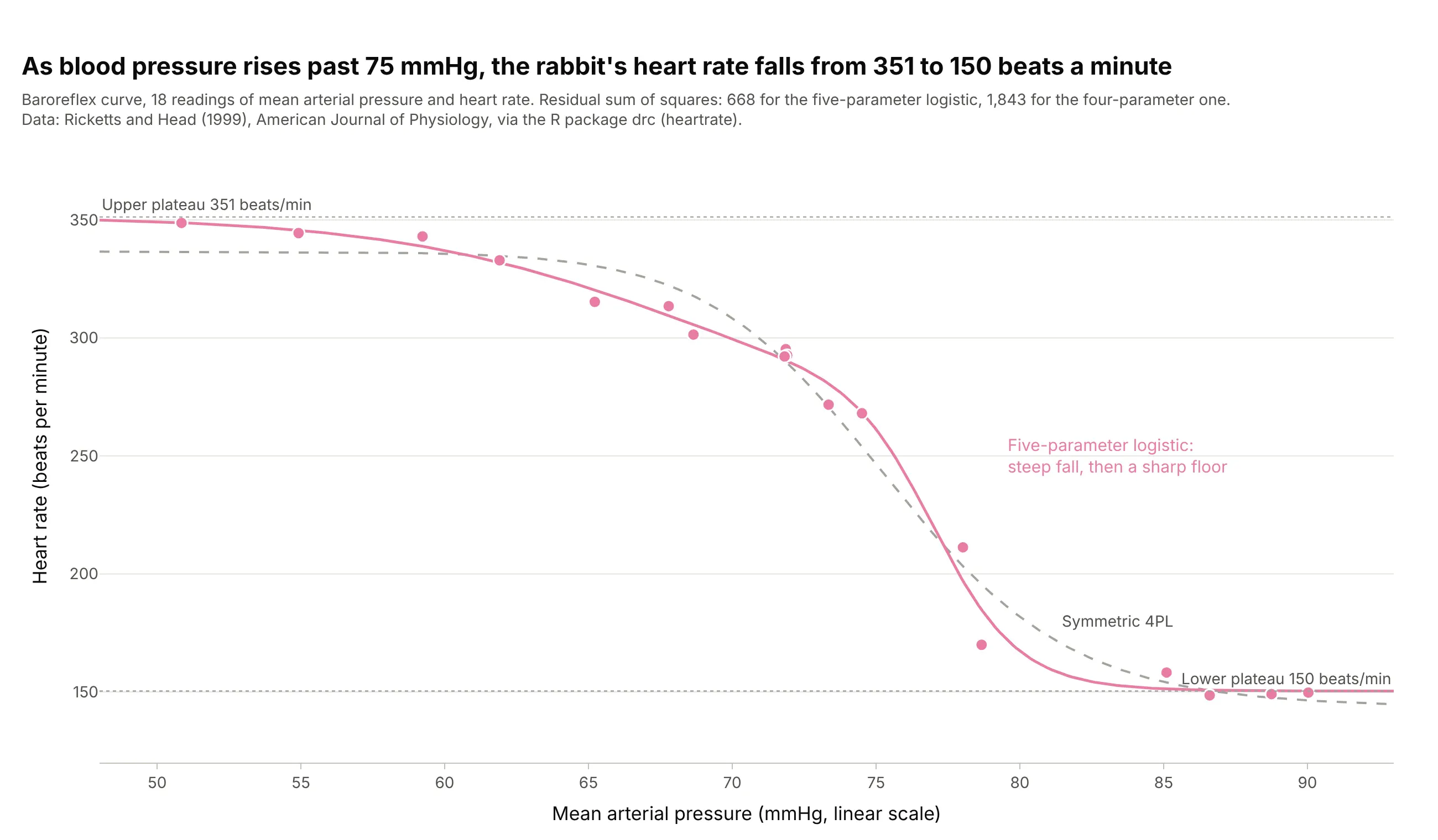
Heart rate of a rabbit against mean arterial pressure on a linear axis from 48 to 93 mmHg: the pink five-parameter logistic falls slowly from a plateau of 351 beats per minute, then steeply after 75 mmHg to a sharp floor at 150, while a dashed symmetric four-parameter logistic misses both bends

As blood pressure rises past 75 mmHg, a rabbit’s heart slows from 351 to 150 beats a minute. The fall bends more sharply at the bottom than at the top, so a five-parameter logistic fits with a residual sum of squares of 668 against 1,843 for the symmetric 4PL. Data: Ricketts and Head (1999), American Journal of Physiology, via the R package drc (heartrate).

Tip: use a linear axis when the “dose” is a physiological variable spread over a narrow range, such as pressure from 50 to 90 mmHg.

Get the data from the R package drc's heartrate dataset (Ricketts and Head 1999, 18 readings of mean arterial
pressure in mmHg and heart rate in beats per minute from a rabbit baroreflex study) and shape it into a table
(columns: pressure_mmhg, heart_rate_bpm).

Build a plotly chart with a five-parameter (baro5) logistic fit and a dashed 4PL for comparison on a linear x
axis, the plateaus labeled and both residual sums of squares in the subtitle.

6. One assay on six days: normalize to each day’s control

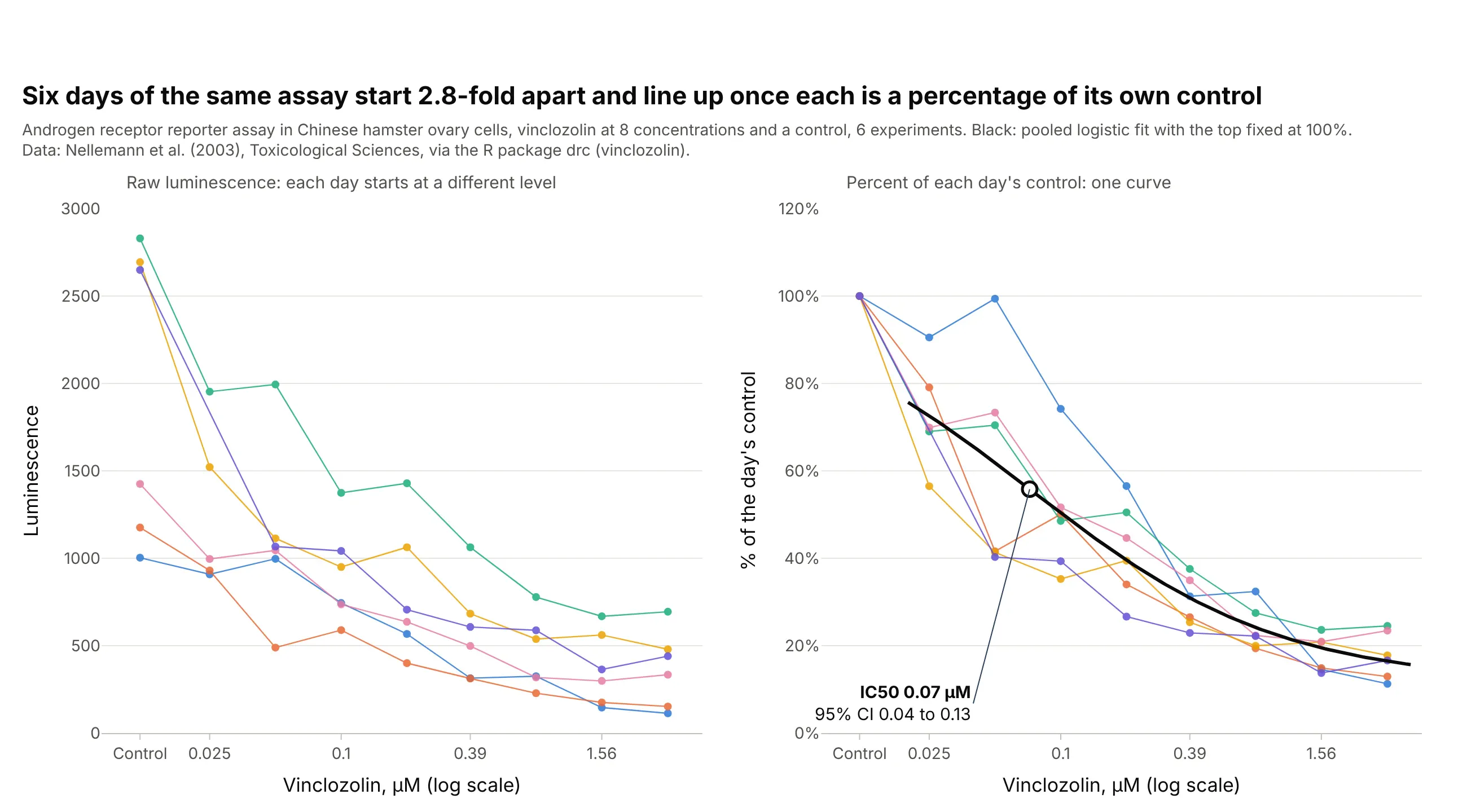
Two panels of an androgen receptor reporter assay with vinclozolin on six days: on the left, raw luminescence where the controls range from about 1,000 to 2,800 and the six colored lines fall in parallel at different heights; on the right, the same data as a percentage of each day’s control, overlapping along one black logistic curve with an IC50 of 0.07 µM

The controls of six runs of the same reporter assay differ 2.8-fold, from 1,003 to 2,830, so the raw curves don’t line up. As a percentage of each day’s control they overlap, and a pooled fit gives an IC50 of 0.07 µM (95% CI 0.04 to 0.13) for the fungicide vinclozolin. Data: Nellemann et al. (2003), Toxicological Sciences, via the R package drc (vinclozolin).

Tip: show the raw and normalized runs side by side once, so readers can trust the normalization.

Get the data from the R package drc's vinclozolin dataset (Nellemann et al. 2003, luminescence of an androgen
receptor reporter assay in Chinese hamster ovary cells at 8 vinclozolin concentrations and a control, 6
experiments) and shape it into a table (columns: experiment, conc_um, luminescence).

Build two plotly panels: raw luminescence by day, and each day as a percentage of its own control with a pooled
logistic fit (top fixed at 100%) and the IC50 with its 95% CI.