Chris Parmer

October 27, 2026

Forest Plots - A Complete Guide

TL;DR

A forest plot puts one estimate per row (a trial, a subgroup, a regression coefficient) with its confidence interval, on a shared axis with a line at "no effect", and often a diamond for the pooled result.
Forest plots are also known as blobbograms, and are similar to dot plots and coefficient plots.
It's the standard figure of meta-analysis and of subgroup results in clinical trials, and it works just as well for regression coefficients, A/B tests and repeated measurements.
Use a log axis for ratios (hazard, odds, risk ratios) so 0.5 and 2 sit the same distance from 1, and size each square by its weight.
You can make a forest plot with Plotly from a go.Scatter with error_x for the rows and a filled scatter for the diamond, and any coding agent can build one in a minute.

What is a forest plot?

Forest plots look like this:

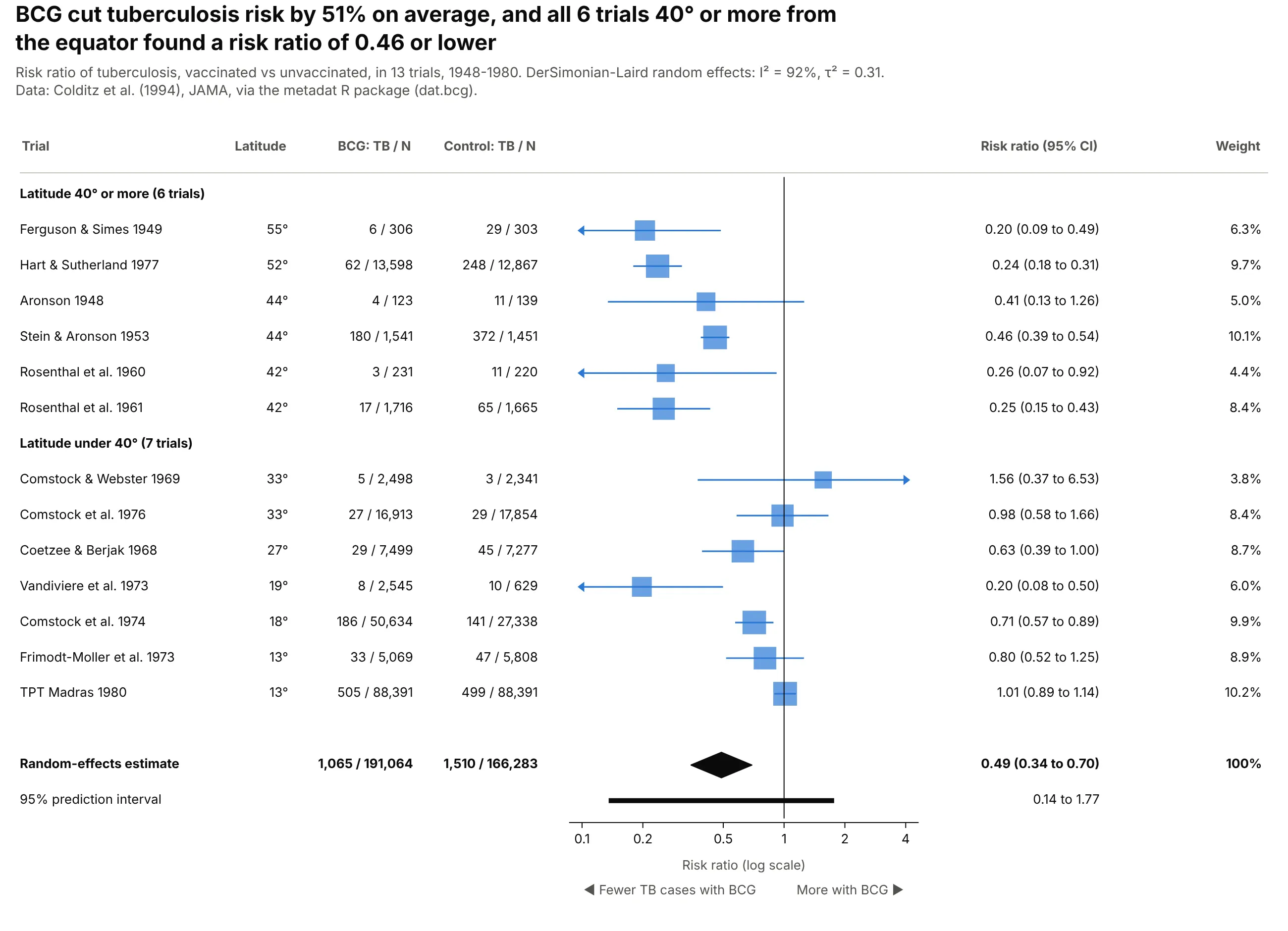
Forest plot of 13 trials of the BCG vaccine against tuberculosis, 1948 to 1980, sorted by latitude, with risk ratios on a log axis, squares sized by weight, a random-effects diamond at 0.49 (0.34 to 0.70) and a 95% prediction interval from 0.14 to 1.77. All six trials 40 degrees or more from the equator found a risk ratio of 0.46 or lower

Data: Colditz et al. (1994), JAMA, via the metadat R package.

How do you read a forest plot? In the example above, notice these things:

Each row is one trial. The blue square is that trial's risk ratio, and the line through it is its 95% confidence interval, so a short line like Stein & Aronson 1953 is a precise result and a long one like Aronson 1948 is a rough one.
The vertical line at 1 means the vaccine made no difference. Squares to its left mean fewer tuberculosis cases with BCG, and a trial whose line crosses 1, like TPT Madras 1980, can't rule out no effect on its own.
The axis is on a log scale, so halving the risk and doubling it sit the same distance from 1. The size of each square shows how much weight that trial gets in the average, and the arrows mark intervals that run off the edge of the axis.
The black diamond at the bottom pools all 13 trials. Its center is the average risk ratio and its width is the confidence interval of that average.
Grouping the rows by latitude shows why the trials disagree, because every trial far from the equator sits well to the left while the ones nearer the equator spread out on both sides of 1. When the rows disagree this much, read the thick prediction interval under the diamond, which crosses 1, as the range a new trial could land in.

It's often used for charts like these:

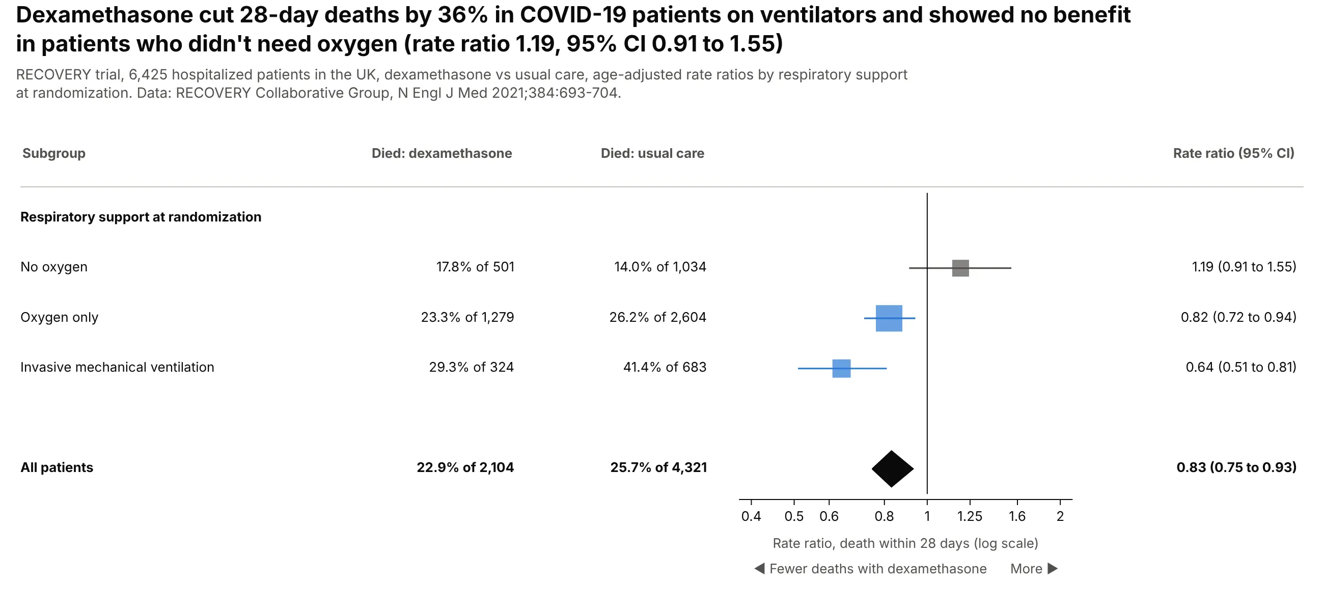
Forest plot of the RECOVERY trial's dexamethasone results by respiratory support: rate ratio 1.19 (0.91 to 1.55) with no oxygen, 0.82 (0.72 to 0.94) with oxygen only, 0.64 (0.51 to 0.81) on invasive ventilation, and 0.83 (0.75 to 0.93) for all 6,425 patients

Subgroups of one trial. Dexamethasone cut 28-day deaths among ventilated COVID-19 patients by 36% (rate ratio 0.64) and showed no benefit for patients who didn't need oxygen (1.19, 95% CI 0.91 to 1.55). Data: RECOVERY Collaborative Group, N Engl J Med 2021.

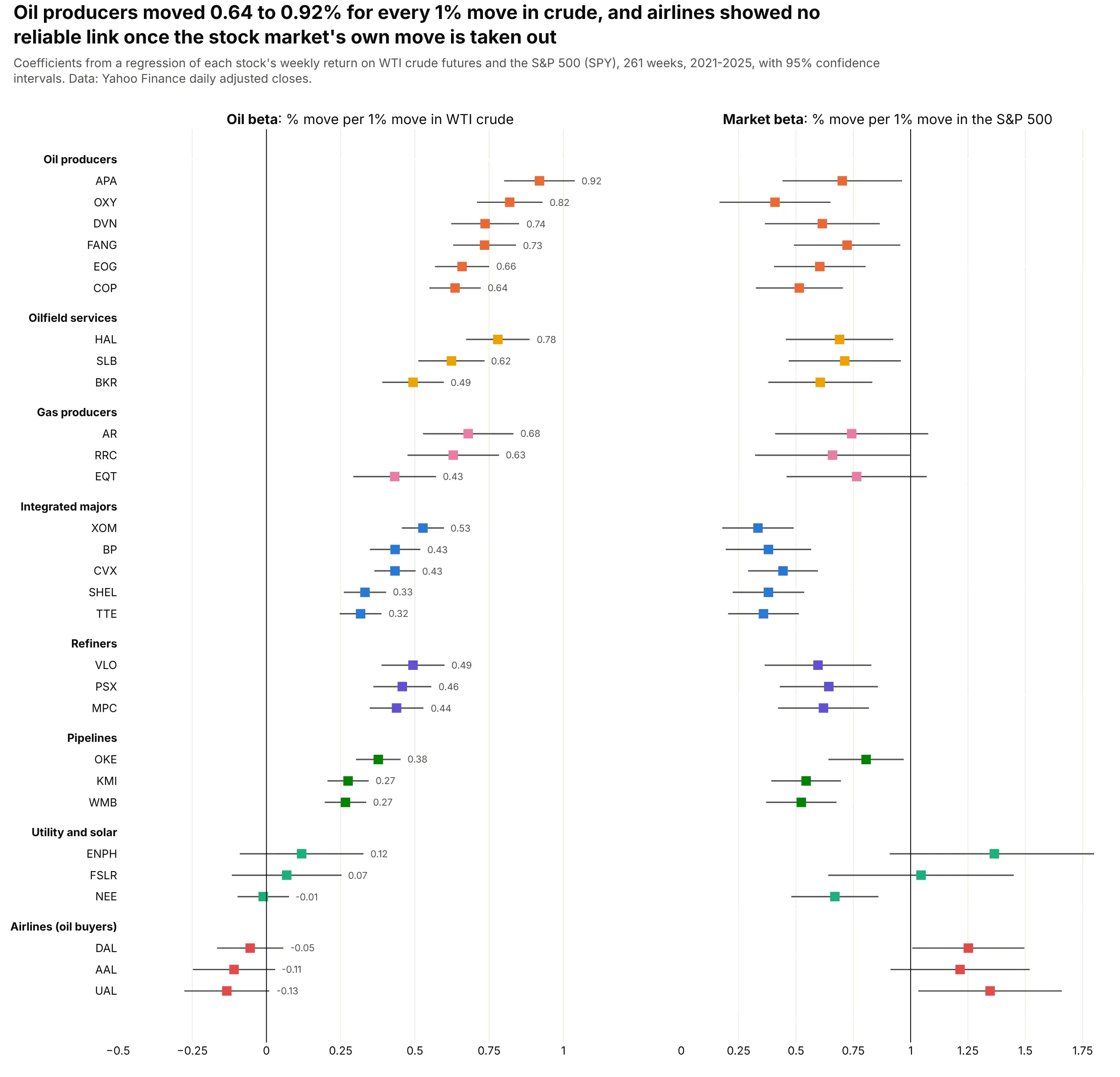
Coefficient plot of the oil beta and market beta of 29 energy, utility and airline stocks, grouped by subsector. Oil producers move 0.64 to 0.92% per 1% move in WTI crude, pipelines 0.27 to 0.38, and airlines -0.05 to -0.13 with intervals that cross zero

Regression coefficients. Over 261 weeks in 2021-2025, oil producers moved 0.64% (ConocoPhillips) to 0.92% (APA) for every 1% move in crude, after taking out the stock market's move. Data: Yahoo Finance, weekly returns.

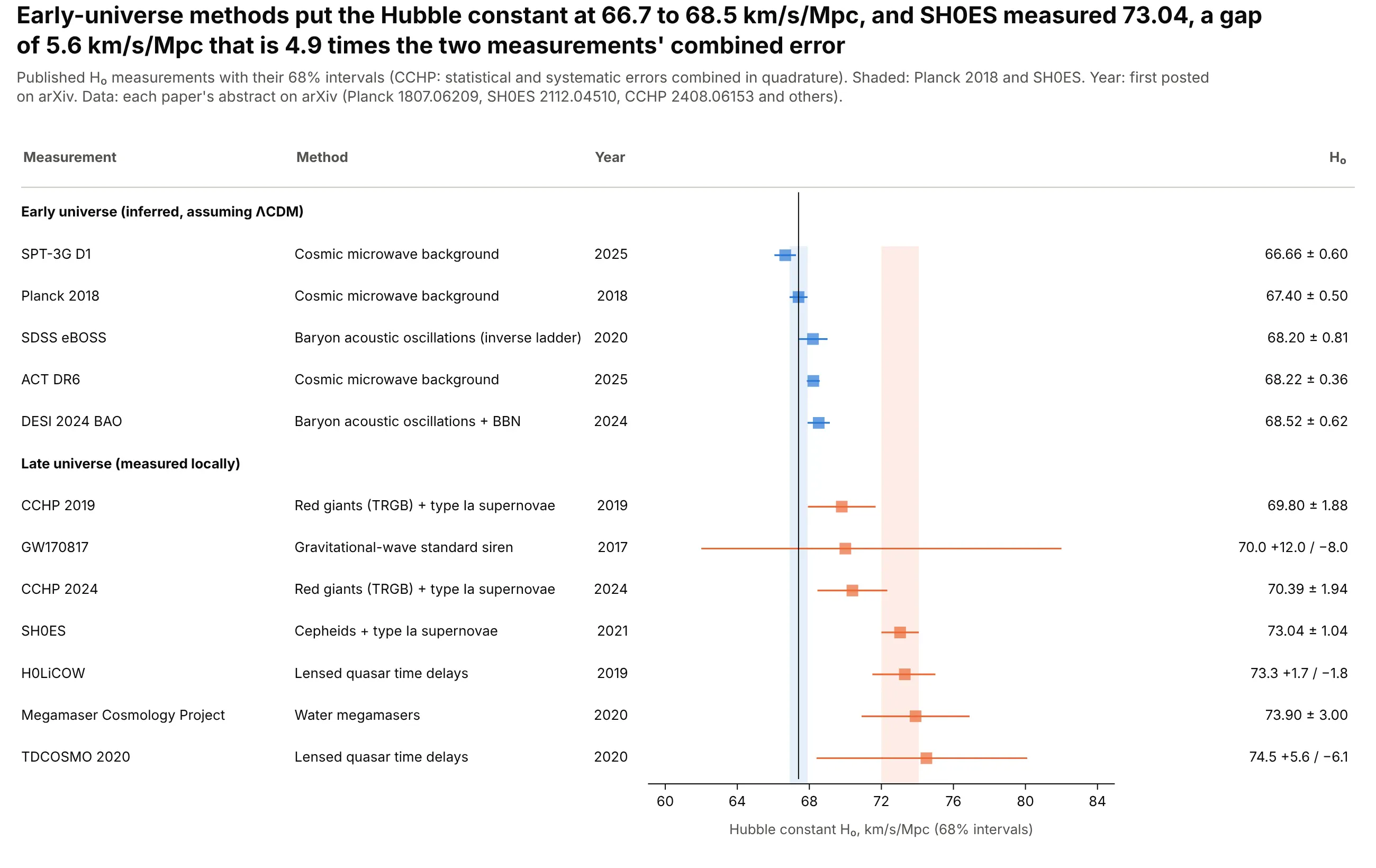
Forest plot of 12 published measurements of the Hubble constant with 68% intervals: five early-universe values from 66.66 to 68.52 km/s/Mpc and seven local measurements, including SH0ES at 73.04, with shaded bands for Planck and SH0ES

Repeated measurements of one quantity. Early-universe methods put the Hubble constant at 66.7 to 68.5 km/s/Mpc, while SH0ES measured 73.04, a gap 4.9 times the two measurements' combined error. Data: the papers' abstracts on arXiv.

A short history

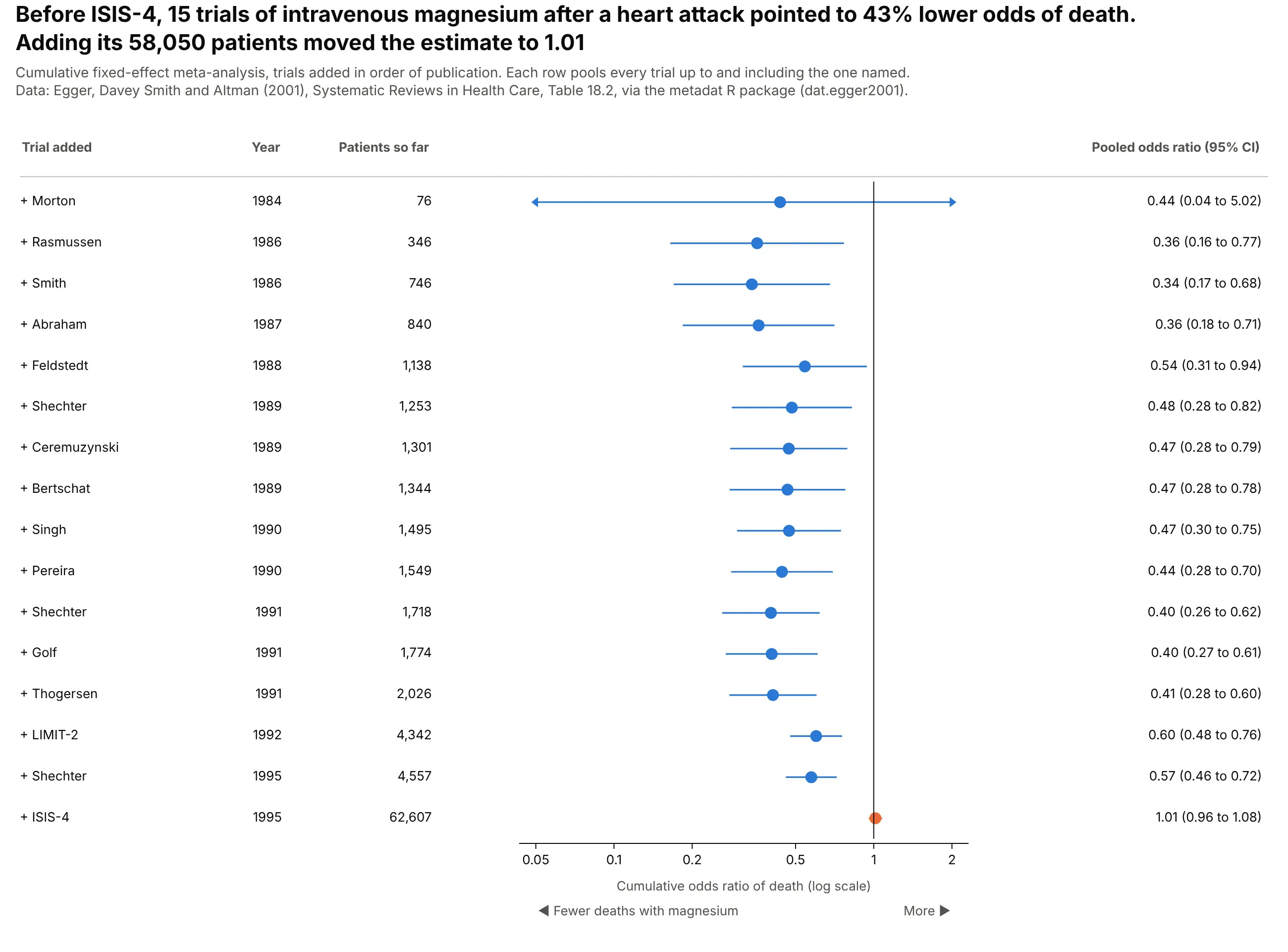
Forest plots became the standard figure of medical meta-analysis, where each row is a trial and the diamond is the combined answer. The random-effects method most of them still use was published by DerSimonian and Laird in 1986, and Lewis and Clarke's 2001 BMJ article explains how to read one. A cumulative forest plot of intravenous magnesium after a heart attack, the case Egger and Davey Smith described in 1995, shows why the format matters: small trials pointed to a large benefit for a decade, and the 58,050-patient ISIS-4 trial erased it.

Cumulative forest plot of 16 trials of intravenous magnesium after a heart attack, 1984 to 1995. The pooled odds ratio of death stays between 0.34 and 0.60 through 15 trials (0.57 after Shechter 1995) and moves to 1.01 (0.96 to 1.08) when ISIS-4 is added

Alternatives to a forest plot

Here's the same 13 BCG trials drawn six ways. Some are better for the question, some worse, some just different:

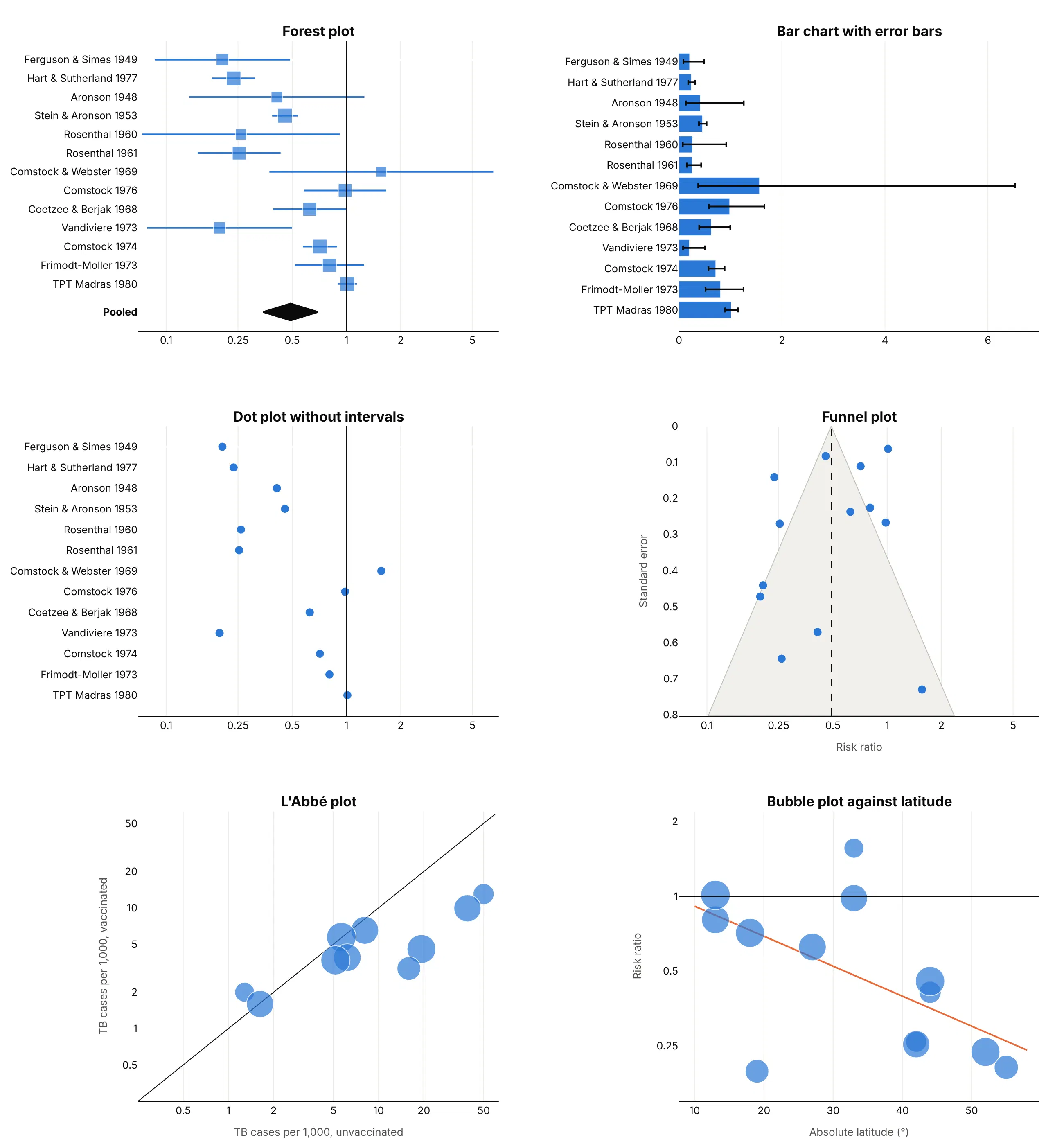
The 13 BCG vaccine trials drawn six ways: a forest plot with a pooled diamond, a bar chart of risk ratios from zero with error bars, a dot plot without intervals, a funnel plot of risk ratio against standard error, a L'Abbé plot of TB risk in vaccinated against unvaccinated groups, and a bubble plot of risk ratio against latitude with a falling trend line

Bar chart with error bars (worse). Bars start at zero, which means nothing for a ratio, and on a linear axis the one wide interval (Comstock and Webster, 0.37 to 6.53) squeezes the rest.
Dot plot without intervals (worse). It shows the estimates but not how sure each one is, so a trial with 14 TB cases (Rosenthal 1960) looks as convincing as one with 310 (Hart and Sutherland, 26,465 people).
Funnel plot (different). Plots each estimate against its standard error to check for small-study and publication bias. Use it next to the forest plot, not instead of it.
L'Abbé plot (different). Plots the event rate in the treated group against the control group, so it shows the baseline risk the forest plot hides. Points below the diagonal favor the vaccine.
Bubble plot against a moderator (better for explaining heterogeneity). Here the risk ratio falls with latitude, which a forest plot can only hint at by sorting. See our bubble chart guide.

How to make a forest plot

With AI

ChatGPT, Claude Code, GitHub Copilot, Cursor and other AI tools are excellent at writing Plotly code. Name Plotly in the prompt, say what each row is and what scale the effect is on, and list the checks you want:

Make a plotly forest plot from trials.csv (columns: trial, year, hr, ci_low, ci_high, n).

- Draw the squares with go.Scatter and the intervals with error_x
  (array = ci_high - hr, arrayminus = hr - ci_low), one row per trial, ordered by year.
- Log x axis with a vertical line at 1; square size by inverse-variance weight.
- Pool the trials with DerSimonian-Laird random effects and draw the result as a filled
  diamond under the rows. Print I² in the subtitle.
- Put a table to the right: "HR (95% CI)" formatted to two decimals.
- Label the axis ends "Favors drug" and "Favors placebo".
- Assert ci_low < hr < ci_high on every row.
- Save it as forest.html and as a PNG at 2x scale.

With Plotly Studio

Plotly Studio is a desktop app where you point an AI at a dataset and it builds charts and a Dash app around your questions. Ask for a forest plot the same way:

Show a forest plot of the trials in this file: hazard ratio with 95% CI on a log axis, a line at 1, squares sized by weight and a random-effects diamond. Add a dropdown to switch between the primary outcome and all-cause death.

Make a forest plot in Python or JavaScript

This is the code AI tools write under the hood. This helper builds a forest plot from go.Scatter and pools the rows with DerSimonian-Laird. Every example in this guide builds on the same idea:

import numpy as np
import plotly.graph_objects as go


def dersimonian_laird(y, v):
    """Random-effects pooling of effects y (log ratios or differences) with variances v."""
    w = 1 / v
    q = np.sum(w * (y - np.sum(w * y) / w.sum()) ** 2)
    tau2 = max(0.0, (q - (len(y) - 1)) / (w.sum() - np.sum(w ** 2) / w.sum()))
    wr = 1 / (v + tau2)
    return np.sum(wr * y) / wr.sum(), np.sqrt(1 / wr.sum()), wr / wr.sum()


def make_forest_plot(df, label, est, lo, hi, weight=None, pooled=None, ref=1, log=True):
    d = df.iloc[::-1].reset_index(drop=True)  # first row at the top
    y, ticks = list(range(len(d))), list(d[label])
    size = 9 if weight is None else 6 + 18 * np.sqrt(d[weight] / d[weight].max())
    fig = go.Figure(go.Scatter(
        x=d[est], y=y, mode="markers", marker=dict(symbol="square", size=size, color="#2a78d6"),
        error_x=dict(type="data", symmetric=False, array=d[hi] - d[est], arrayminus=d[est] - d[lo], width=0)))
    if pooled:  # (estimate, low, high) as a diamond under the rows
        m, l, h = pooled
        fig.add_scatter(x=[l, m, h, m, l], y=[-1.5, -1.1, -1.5, -1.9, -1.5], mode="lines",
                        fill="toself", fillcolor="#0b0b0b", line_color="#0b0b0b")
        y, ticks = [-1.5] + y, ["<b>Pooled</b>"] + ticks
    fig.add_scatter(x=[ref, ref], y=[min(y) - 0.6, len(d) - 0.4], mode="lines", line=dict(color="#0b0b0b", width=1))
    fig.update_layout(template="simple_white", showlegend=False,
                      xaxis=dict(type="log" if log else "linear"), yaxis=dict(tickvals=y, ticktext=ticks))
    return fig


# y = log risk ratios, v = their variances, df has label, rr, lo, hi:
# mu, se, df["w"] = dersimonian_laird(y, v)
# fig = make_forest_plot(df, "label", "rr", "lo", "hi", weight="w",
#                        pooled=(np.exp(mu), np.exp(mu - 1.96 * se), np.exp(mu + 1.96 * se)))

In JavaScript, plotly.js builds the same thing from three scatter traces:

<div id="chart" style="height:420px"></div>
<script src="https://cdn.plot.ly/plotly-4.1.1.min.js"></script>
<script>
  const rr = [1.19, 0.82, 0.64], lo = [0.91, 0.72, 0.51], hi = [1.55, 0.94, 0.81];
  Plotly.newPlot("chart", [
    { type: "scatter", mode: "markers", x: rr, y: [1, 2, 3],
      marker: { symbol: "square", size: 14, color: "#2a78d6" },
      error_x: { type: "data", symmetric: false, width: 0,
                 array: hi.map((h, i) => h - rr[i]), arrayminus: lo.map((l, i) => rr[i] - l) } },
    { type: "scatter", mode: "lines", fill: "toself", fillcolor: "#0b0b0b", line: { color: "#0b0b0b" },
      x: [0.75, 0.83, 0.93, 0.83, 0.75], y: [0, -0.3, 0, 0.3, 0] },
    { type: "scatter", mode: "lines", x: [1, 1], y: [-0.6, 3.6], line: { color: "#0b0b0b", width: 1 } }
  ], {
    showlegend: false,
    xaxis: { type: "log", tickvals: [0.5, 0.75, 1, 1.5], title: { text: "Rate ratio (log scale)" } },
    yaxis: { zeroline: false, autorange: "reversed", tickvals: [0, 1, 2, 3],
             ticktext: ["<b>All patients</b>", "No oxygen", "Oxygen only", "Ventilated"] }
  });
</script>

Share it

Every Plotly chart has a Share chart button (the cloud icon in its toolbar) that uploads it to Plotly Cloud and gives you a link. Only you can see it until you change its visibility.

For a live app, put the chart in a Dash app and publish it with the Plotly Cloud CLI. Coding agents can run these commands for you:

pip install "dash[cloud]"
plotly user login
plotly app publish

If your data has to stay in your own cloud or data center, publish to Dash Enterprise instead.

Dos and don'ts

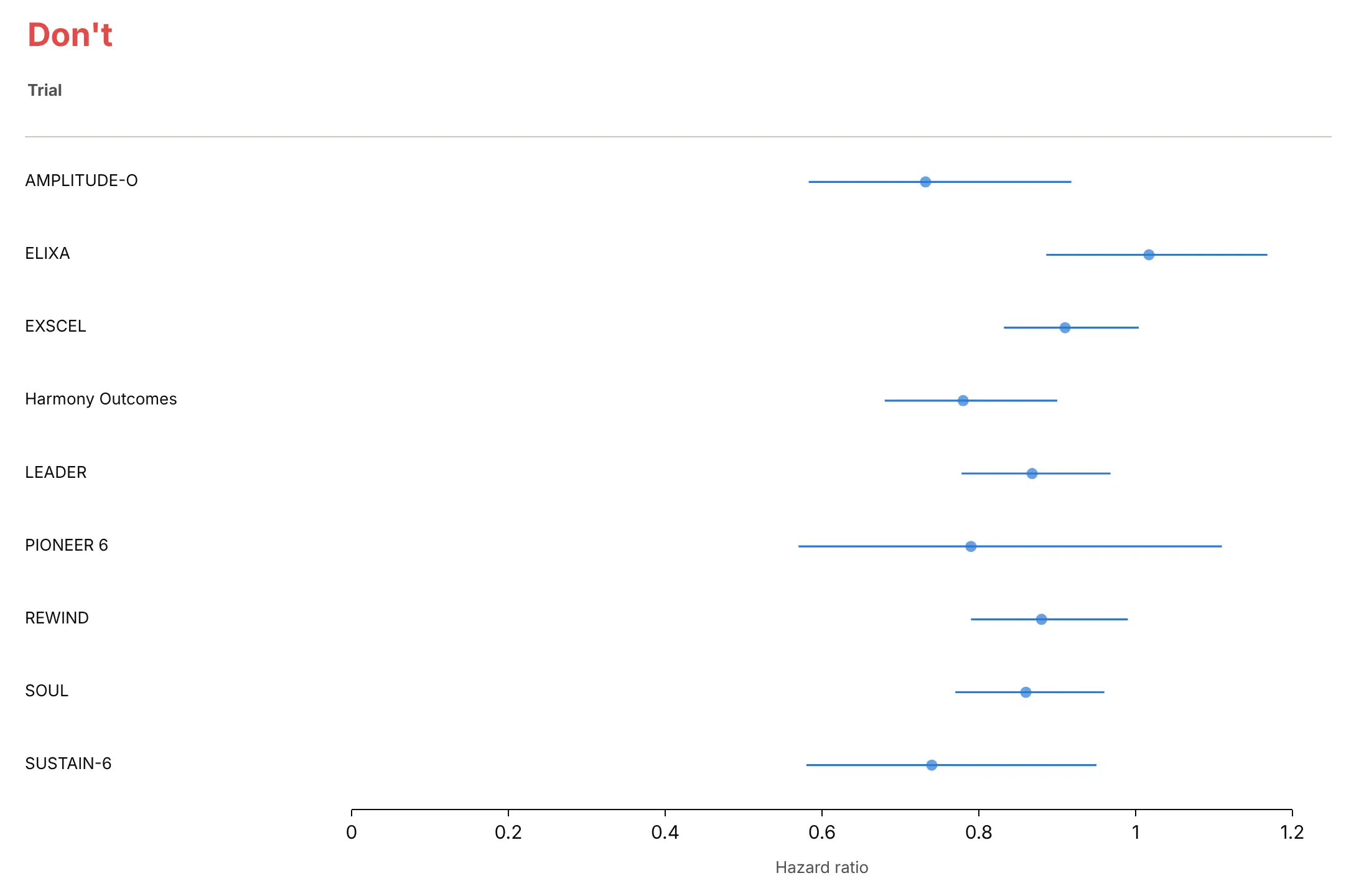
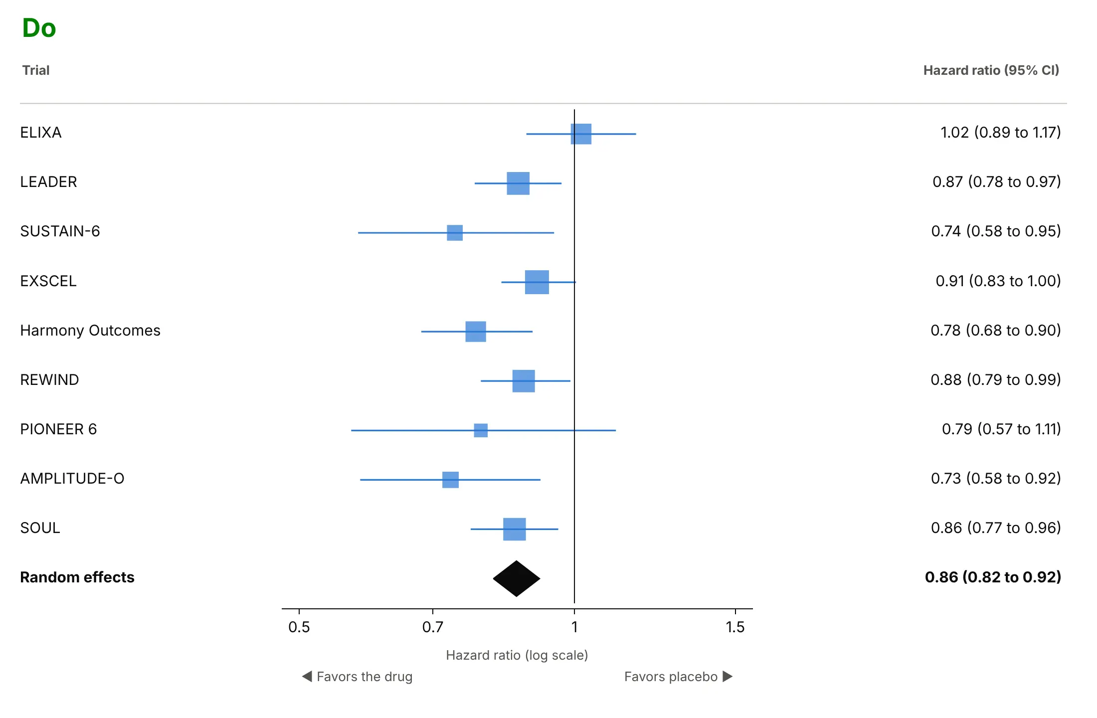
A forest plot is read by scanning the rows against the line of no effect, so most mistakes are about the axis, the order and what's missing. Here are nine GLP-1 heart trials both ways.

Don't list the rows alphabetically on a linear axis from zero, leave out the line at 1, draw every trial with the same marker and skip the numbers and the pooled result:

The nine GLP-1 trials as equal blue dots with confidence intervals, in alphabetical order on a linear axis from 0 to 1.2, with no line at 1, no numbers and no pooled estimate

Do order the rows by something meaningful (here, the date), use a log axis with a line at 1, size squares by weight, print the numbers and add the diamond:

The same nine trials ordered by completion date on a log axis from 0.5 to 1.5 with a line at 1, squares sized by weight, hazard ratios printed on the right and a random-effects diamond at 0.86 (0.82 to 0.92)

Choose what the color says

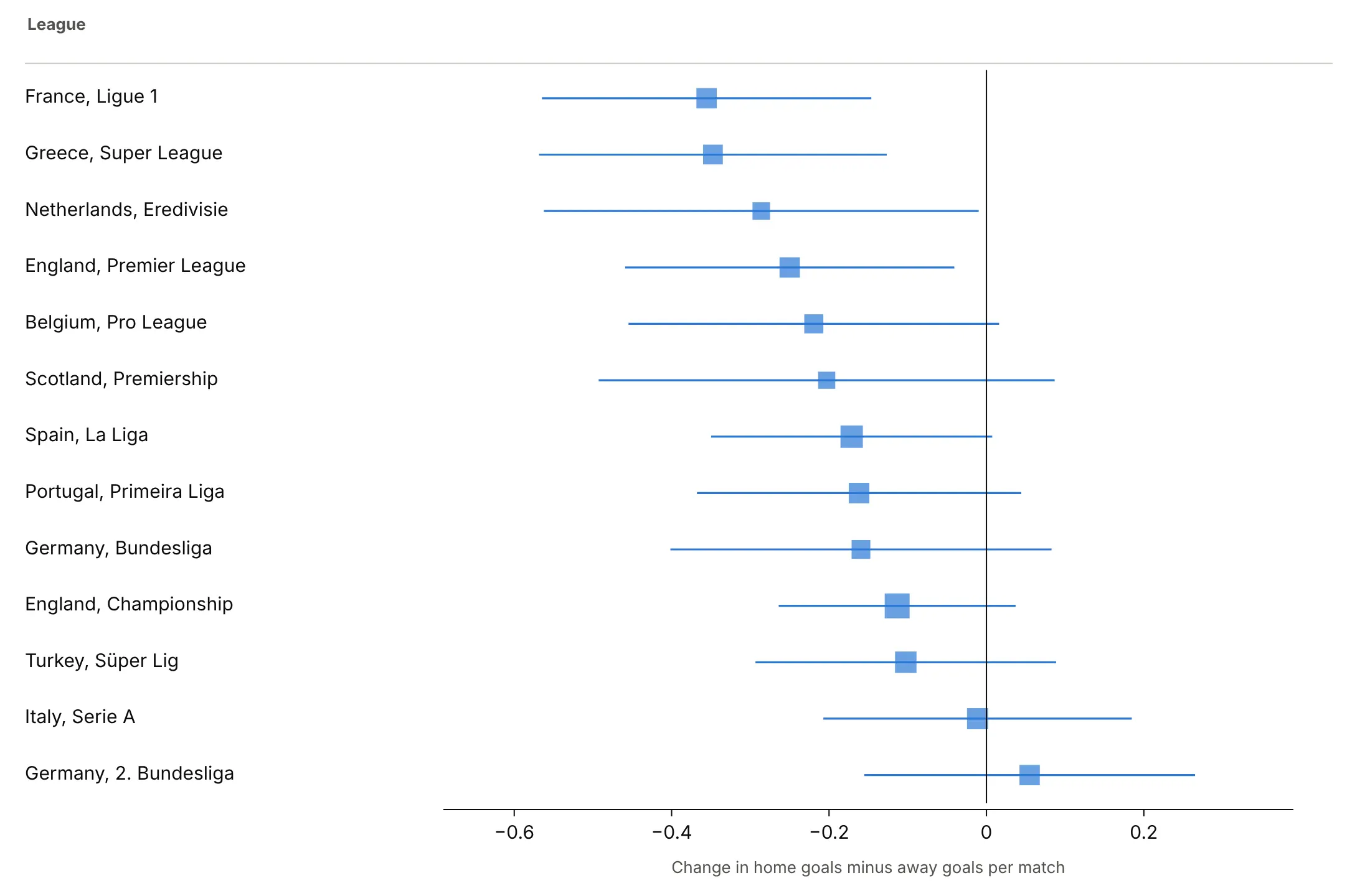
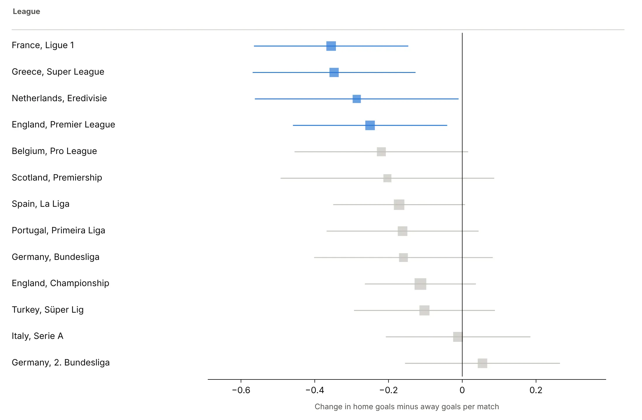
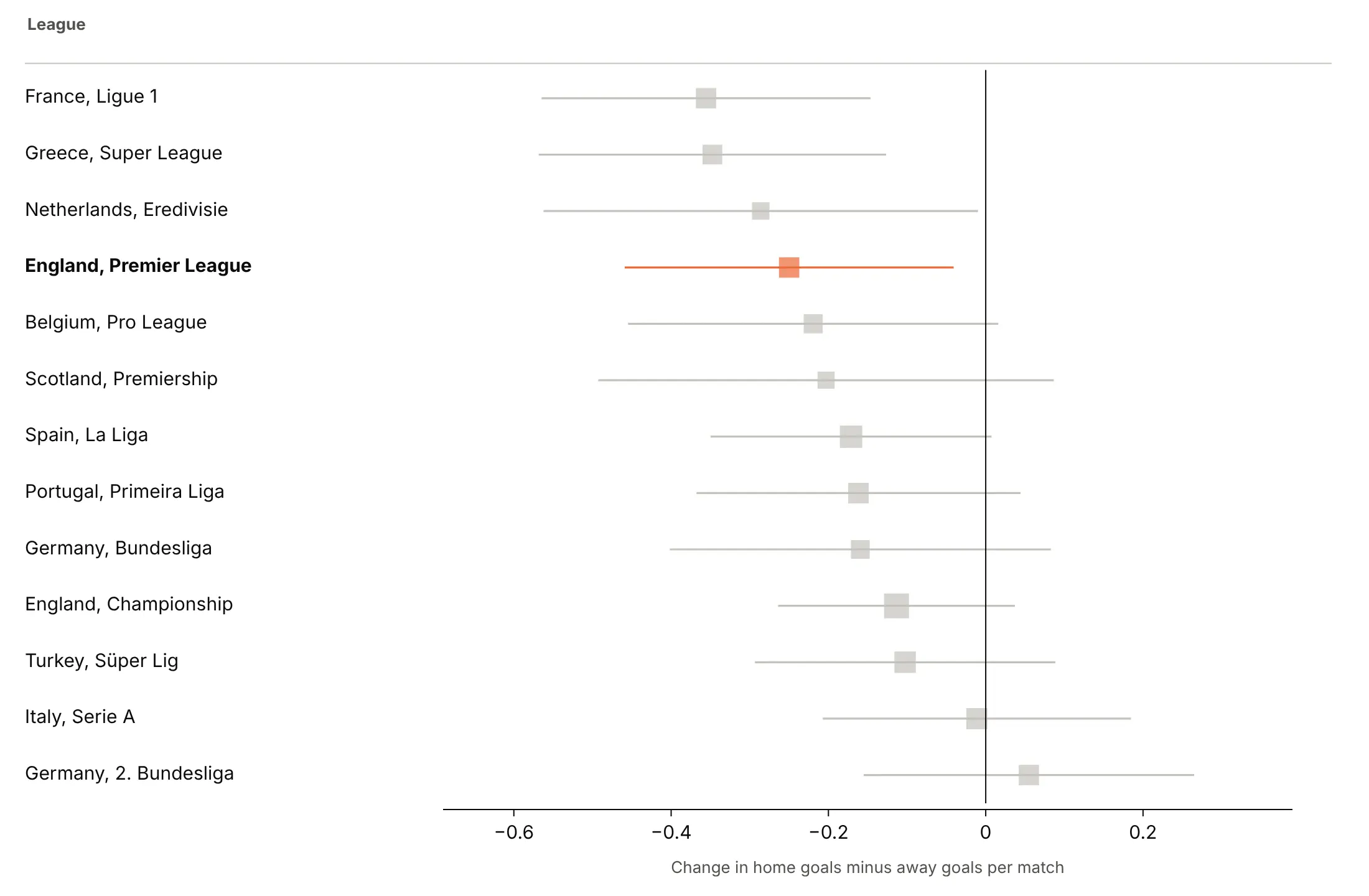
Here are three ways to color the change in home advantage when 13 football leagues played without crowds.

One color, sorted by the estimate. A good default when the order is the message.

Forest plot of 13 European football leagues sorted by the change in home goal difference without crowds, all in blue, from Ligue 1 at -0.36 to 2. Bundesliga at +0.05

Color by verdict. Blue where the interval excludes zero shows that only four leagues clear it on their own.

The same plot with four leagues in blue whose intervals sit entirely below zero, France, Greece, the Netherlands and the Premier League, and the other nine in gray

Highlight one row. For an audience that cares about one league, make it the only color.

The same plot with the Premier League in orange and bold at -0.25 and every other league in gray

Checklist

Use a log axis for ratios and a linear axis for differences, with a line at no effect.
Order rows by something that means something: date, size, a moderator or the estimate.
Size squares by weight so the eye goes to the trials that count.
Print the estimate and interval for every row, formatted to two decimals.
Label which side favors which group, and say what the interval is (95% CI, 68%, credible).

Don't

Start the axis at zero or use bars; a ratio of 1 is the reference, not 0.
Pool studies that measure different things, or put a diamond on a caterpillar of unrelated trials.
Read a subgroup as different just because its interval crosses 1 and another doesn't; test the difference.
Let an axis range cut intervals silently; end them in an arrow.

Options to customize

These are the go.Scatter and layout options that build a forest plot in Plotly. The full list is in the Plotly scatter reference and the error bars documentation.

error_x.array, error_x.arrayminus: the distance from the estimate to the upper and lower limits; set symmetric=False for asymmetric intervals.
error_x.width: the caps at the ends; 0 gives clean lines.
error_x.thickness, error_x.color: line weight and color of the intervals.
marker.symbol="square": the classic square; use circles for rows that aren't weighted studies.
marker.size as a list: square size by weight (use the square root so area tracks weight).
marker.color as a list: color by verdict, subgroup or a highlight.
fill="toself" on a closed go.Scatter: the pooled diamond, with its width as the interval.
xaxis.type="log": the right scale for hazard, odds and risk ratios.
xaxis.tickvals: readable ticks on a log axis (0.5, 1, 2).
yaxis.tickvals, ticktext: row labels at numeric positions, which leaves room for headers and diamonds.
yaxis.autorange="reversed": first row at the top.
mode="text" traces on a second x axis (xaxis2 with domain=[0, 1]): the table of numbers beside the chart.
fig.add_annotation: "favors" labels under the axis and arrows for clipped intervals.
make_subplots(shared_yaxes=True): two coefficient panels on the same rows.
hovertemplate, customdata: show the interval and the weight on hover.

More forest plot examples

Nine more forest plots built from real public data, each with its source, the technique that makes it work and a prompt to rebuild it.

1. GLP-1 drugs and heart attacks, strokes and cardiovascular deaths

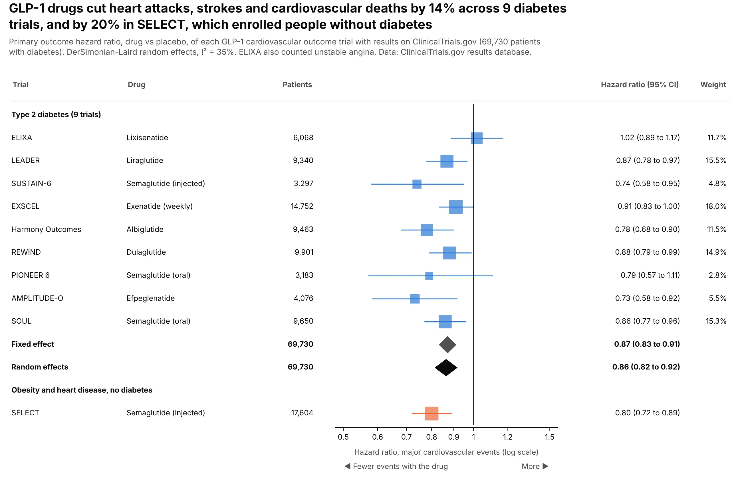
Forest plot of nine GLP-1 receptor agonist cardiovascular outcome trials in type 2 diabetes with a fixed-effect diamond at 0.87 and a random-effects diamond at 0.86 (0.82 to 0.92), and SELECT in orange below at 0.80 (0.72 to 0.89)

Across nine trials in 69,730 people with type 2 diabetes, GLP-1 drugs cut major cardiovascular events by 14% (random effects 0.86, 0.82 to 0.92). SELECT, in people with obesity but no diabetes, found 0.80 and stays out of the pool. Data: ClinicalTrials.gov results database.

Tip: show both the fixed-effect and random-effects diamonds when I² is moderate (35% here), so readers see the choice doesn't change the answer.

Get the data from the ClinicalTrials.gov API v2 (results section, first primary outcome and its
hazard ratio analysis) for ELIXA, LEADER, SUSTAIN-6, EXSCEL, Harmony Outcomes, REWIND, PIONEER 6,
AMPLITUDE-O, SOUL and SELECT
and shape it into a table (columns: trial, drug, population, n_drug, n_placebo, hr, ci_low, ci_high, primary_completion).

Build a plotly forest plot ordered by completion date, log axis, line at 1.
- Back out each SE from the CI; pool the diabetes trials with fixed and DerSimonian-Laird random effects.
- Two diamonds, then SELECT in its own group in orange, not pooled.
- Table columns: drug, patients, HR (95% CI), weight.

2. SGLT2 inhibitors in heart failure, by ejection fraction

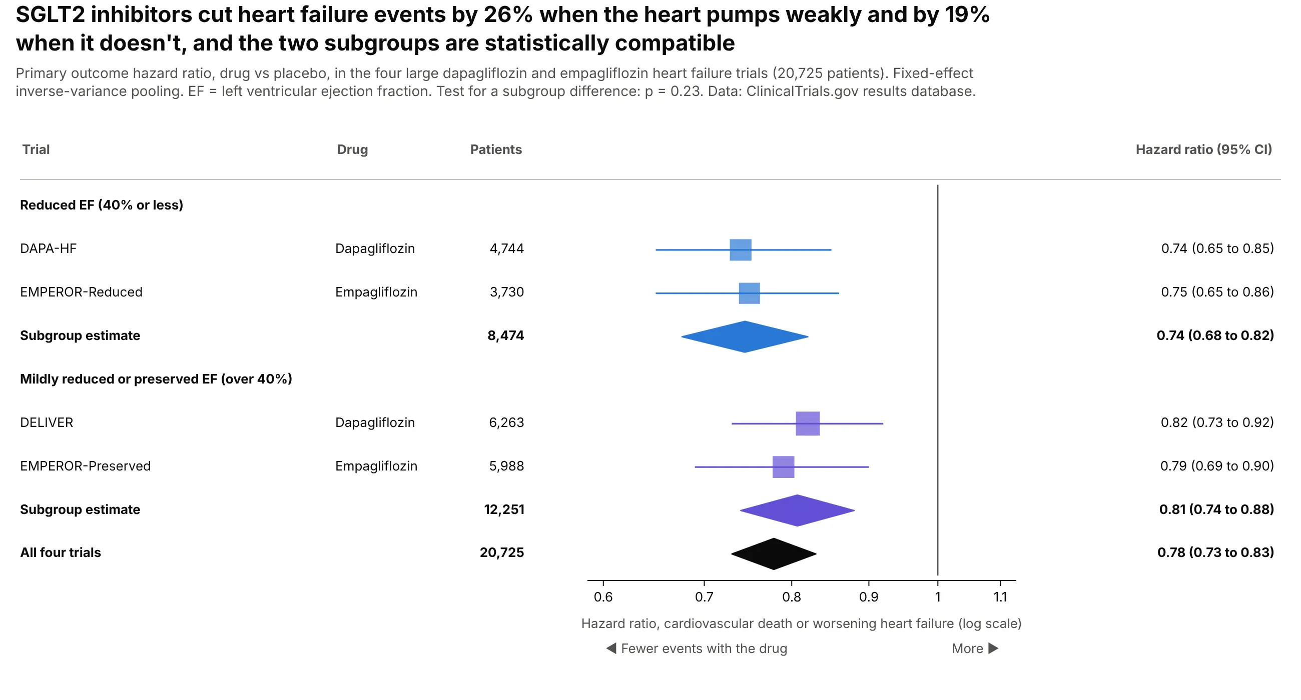
$Forest plot of four SGLT2 inhibitor heart failure trials in two subgroups: reduced ejection fraction pooled at 0.74 (0.68 to 0.82) in blue and mildly reduced or preserved at 0.81 (0.74 to 0.88) in purple, with all four at 0.78$

Dapagliflozin and empagliflozin cut cardiovascular death or worsening heart failure by 26% when ejection fraction was 40% or less and by 19% above it. The test for a difference between subgroups gives p = 0.23. Data: ClinicalTrials.gov results database.

Tip: give each subgroup its own color and its own diamond, and put the test for a difference in the subtitle.

Get the data from the ClinicalTrials.gov API v2 (first primary outcome hazard ratio) for DAPA-HF,
EMPEROR-Reduced, DELIVER and EMPEROR-Preserved
and shape it into a table (columns: trial, drug, ef_group, n_drug, n_placebo, hr, ci_low, ci_high).

Build a plotly forest plot with a header row per ef_group, a fixed-effect diamond per group in the
group's color, and a black diamond for all four. Compute the between-subgroup Q test and print its p.

3. Pfizer-BioNTech vaccine efficacy by subgroup

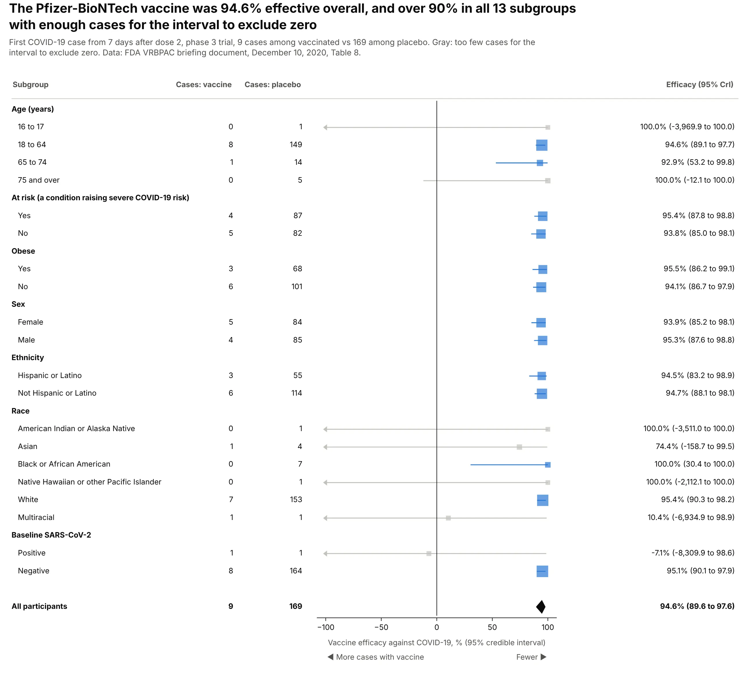
Forest plot of vaccine efficacy in 20 subgroups on a linear axis from -100% to 100%, with 13 blue rows near 95% and seven gray rows whose credible intervals run off the left edge, ending in arrows, and the overall diamond at 94.6%

Efficacy was 94.6% overall and over 90% in all 13 subgroups with enough cases for the interval to exclude zero. The gray rows aren't evidence of failure: the multiracial subgroup had one case in each arm. Data: FDA VRBPAC briefing document, December 10, 2020, Table 8.

Tip: cap the axis at a sensible limit and end longer intervals in an arrow, or one row with a lower bound of -8,310% flattens all the others.

Get the data from the FDA VRBPAC briefing document for the Pfizer-BioNTech COVID-19 vaccine
(December 10, 2020), Table 8
and shape it into a table (columns: group, subgroup, cases_vaccine, cases_placebo, ve, ve_low, ve_high).

Build a plotly forest plot on a linear axis from -100 to 100% with a line at 0.
- Header row per group; square size by total cases; gray where ve_low <= 0.
- Clip intervals at -100% and draw a triangle-left marker where they continue.
- Table: cases per arm and "94.6% (89.6 to 97.6)". Overall result as a diamond.

4. Hydroxychloroquine for COVID-19

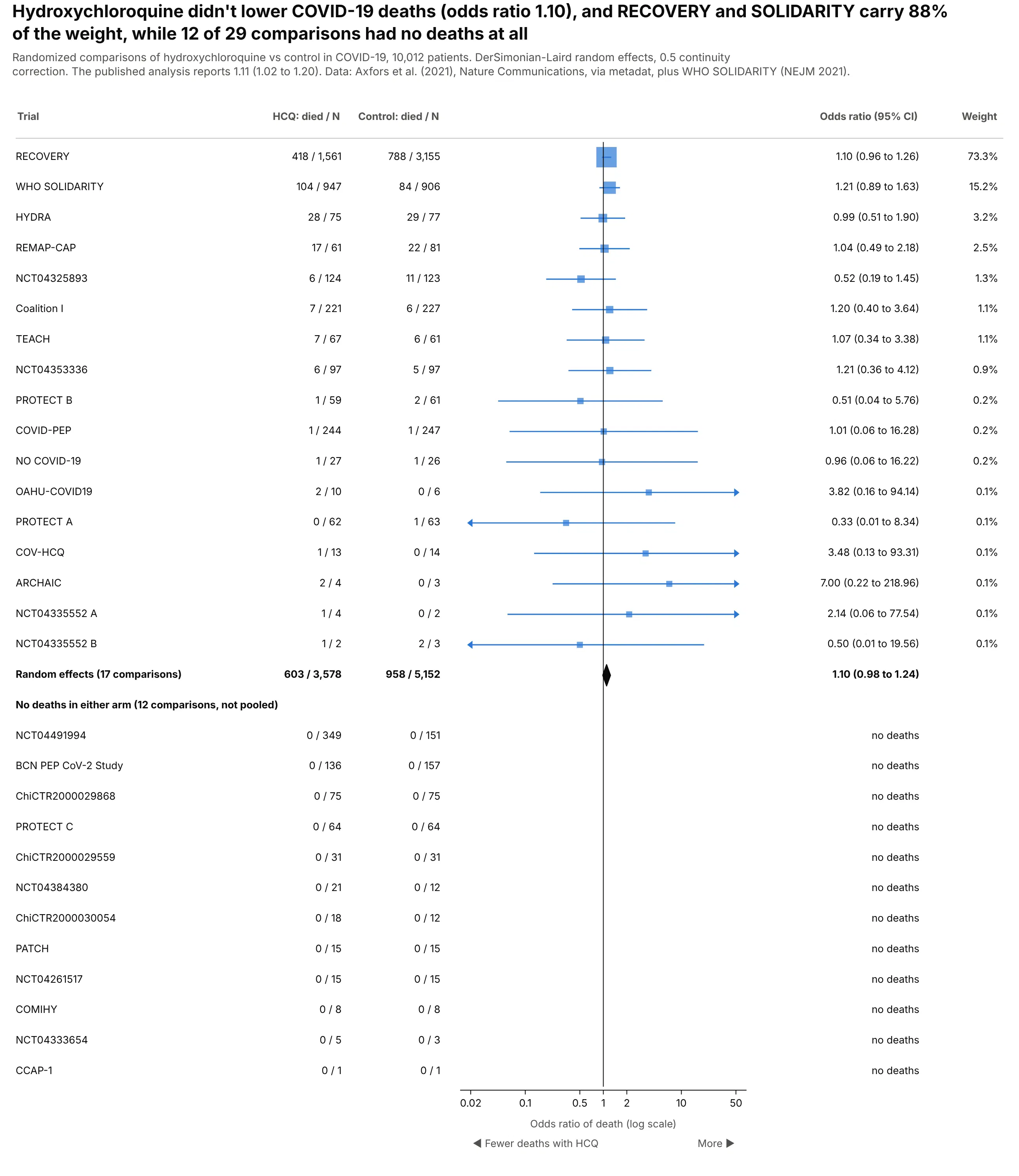
Forest plot of 29 randomized comparisons of hydroxychloroquine against control, sorted by weight: RECOVERY 1.10 (73.3%) and WHO SOLIDARITY 1.21 (15.2%) at the top, 15 small trials with wide intervals, the random-effects diamond at 1.10 (0.98 to 1.24), and 12 trials with no deaths listed below

The 29 comparisons pool to an odds ratio of 1.10 (0.98 to 1.24), and RECOVERY and SOLIDARITY carry 88% of the weight. Twelve trials had no deaths in either arm and can't contribute an odds ratio. The published analysis reports 1.11 (1.02 to 1.20). Data: Axfors et al. (2021), Nature Communications, via metadat, plus WHO SOLIDARITY.

Tip: sort by weight and list zero-event trials below the diamond, so readers see what was left out of the pool and why.

Get the data from the metadat R package dataset dat.axfors2021 (Axfors et al. 2021, deaths per arm in
COVID-19 trials of hydroxychloroquine) plus the WHO SOLIDARITY hydroxychloroquine arm (NEJM 2021)
and shape it into a table (columns: trial, hcq_deaths, hcq_n, control_deaths, control_n).

Build a plotly forest plot of odds ratios on a log axis, sorted by random-effects weight.
- 0.5 continuity correction where one arm has no deaths; trials with none in either arm listed under
  the diamond with "no deaths".
- Table: deaths/N per arm, OR (95% CI), weight.

5. Every phase 3 lung cancer trial with an overall survival result

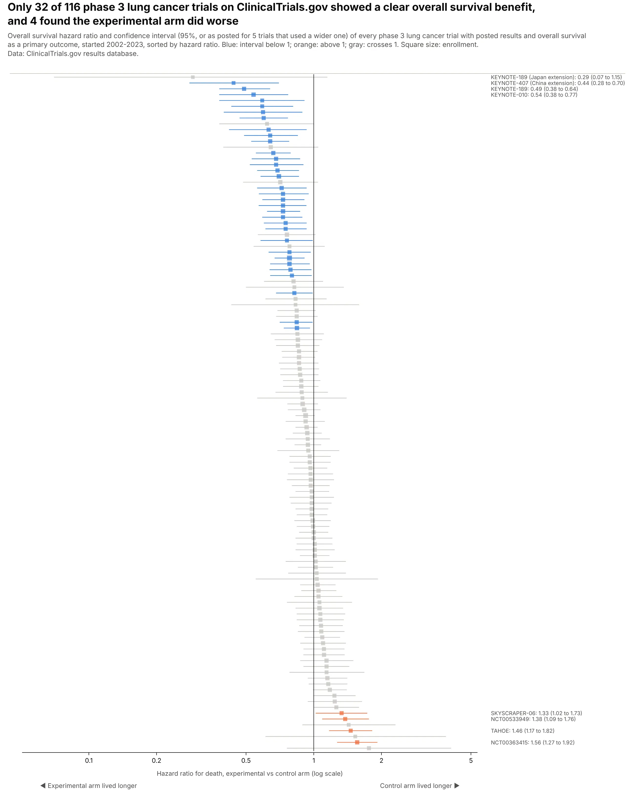
Caterpillar plot of 116 overall survival hazard ratios from phase 3 lung cancer trials, sorted from 0.29 to 1.76: 32 blue rows with intervals below 1 near the top, four orange rows above 1 at the bottom and the rest in gray

Of 116 phase 3 lung cancer trials on ClinicalTrials.gov with an overall survival hazard ratio, 32 showed a clear benefit and 4 found the experimental arm did worse. These trials test different drugs, so there's no diamond. Data: ClinicalTrials.gov results database.

Tip: with over 100 rows, drop the table, sort by the estimate and label only the extremes.

Get the data from the ClinicalTrials.gov API v2: phase 3 interventional studies with results and
condition "lung cancer", the first primary outcome mentioning overall survival with a hazard ratio
and shape it into a table (columns: nct_id, acronym, title, sponsor, start_year, enrollment, hr, ci_low, ci_high, ci_pct).

Build a plotly caterpillar forest plot: one thin row per trial sorted by hr, log axis, line at 1.
- Blue where ci_high < 1, orange where ci_low > 1, gray otherwise; square size by enrollment.
- Label the four lowest and every orange row in a column to the right. No pooled estimate.

6. The value premium, decade by decade

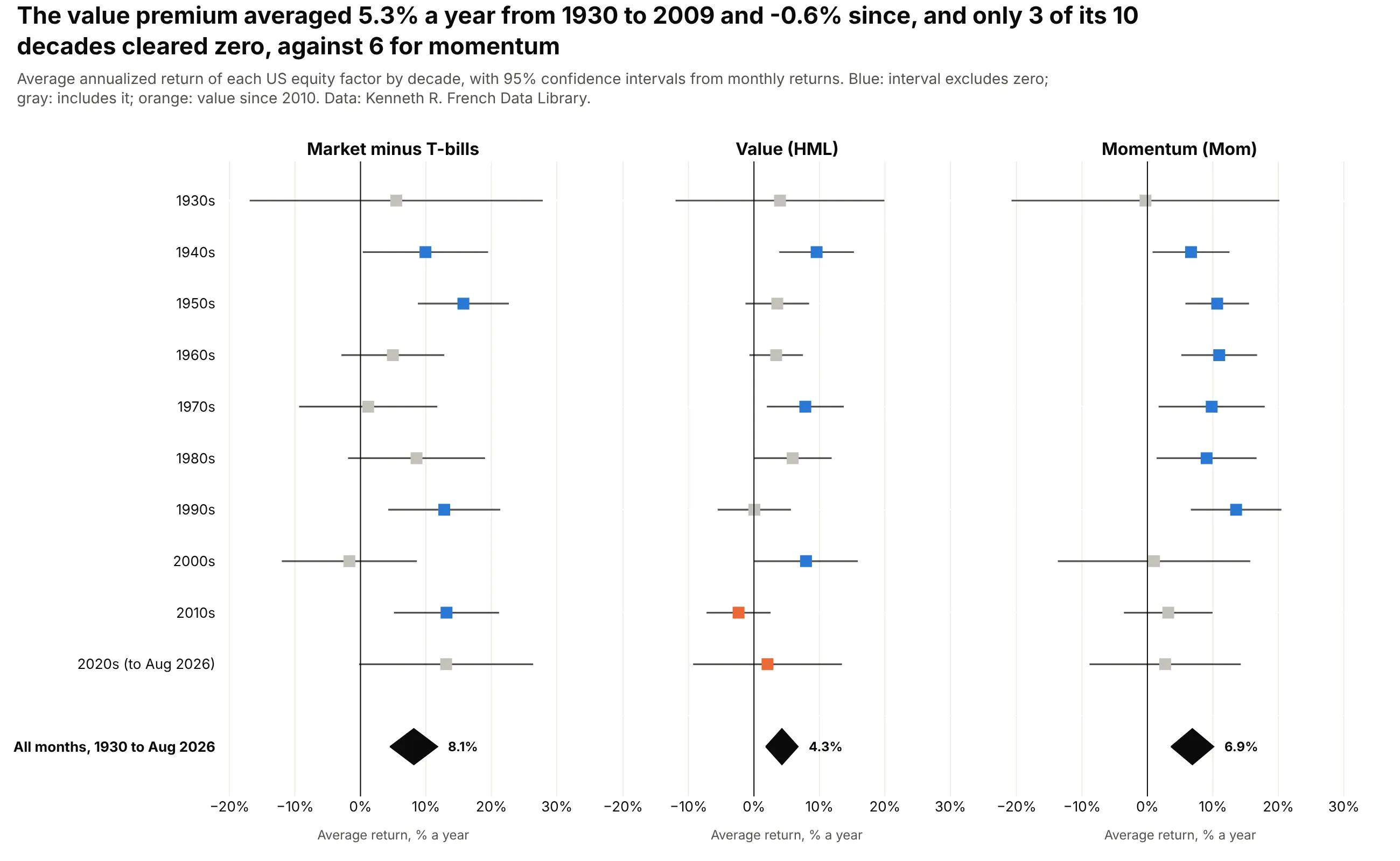
Three panels of annualized factor returns by decade from the 1930s to the 2020s with 95% confidence intervals: market, value and momentum, with value's 2010s (-2.3%) and 2020s (2.1%) in orange and diamonds for the whole period at 8.1%, 4.3% and 6.9%

The value premium averaged 5.3% a year from 1930 to 2009 and -0.6% since, and only 3 of its 10 decades have an interval that clears zero on its own, against 6 for momentum. Data: Kenneth R. French Data Library.

Tip: small multiples with shared rows let readers compare one decade across factors without a legend.

Get the data from Kenneth French's Data Library (F-F_Research_Data_Factors and F-F_Momentum_Factor,
monthly CSVs)
and shape it into a table (columns: month, mkt_rf, smb, hml, mom), returns in % per month.

Build three plotly forest plot panels (make_subplots, shared y) for mkt_rf, hml and mom:
one row per decade from the 1930s, annualized mean (x12) with a 95% CI (1.96 SE x 12),
a line at 0 and a diamond for the whole period. Blue if the CI excludes 0, gray otherwise.

7. How much each grid's demand rises with heat

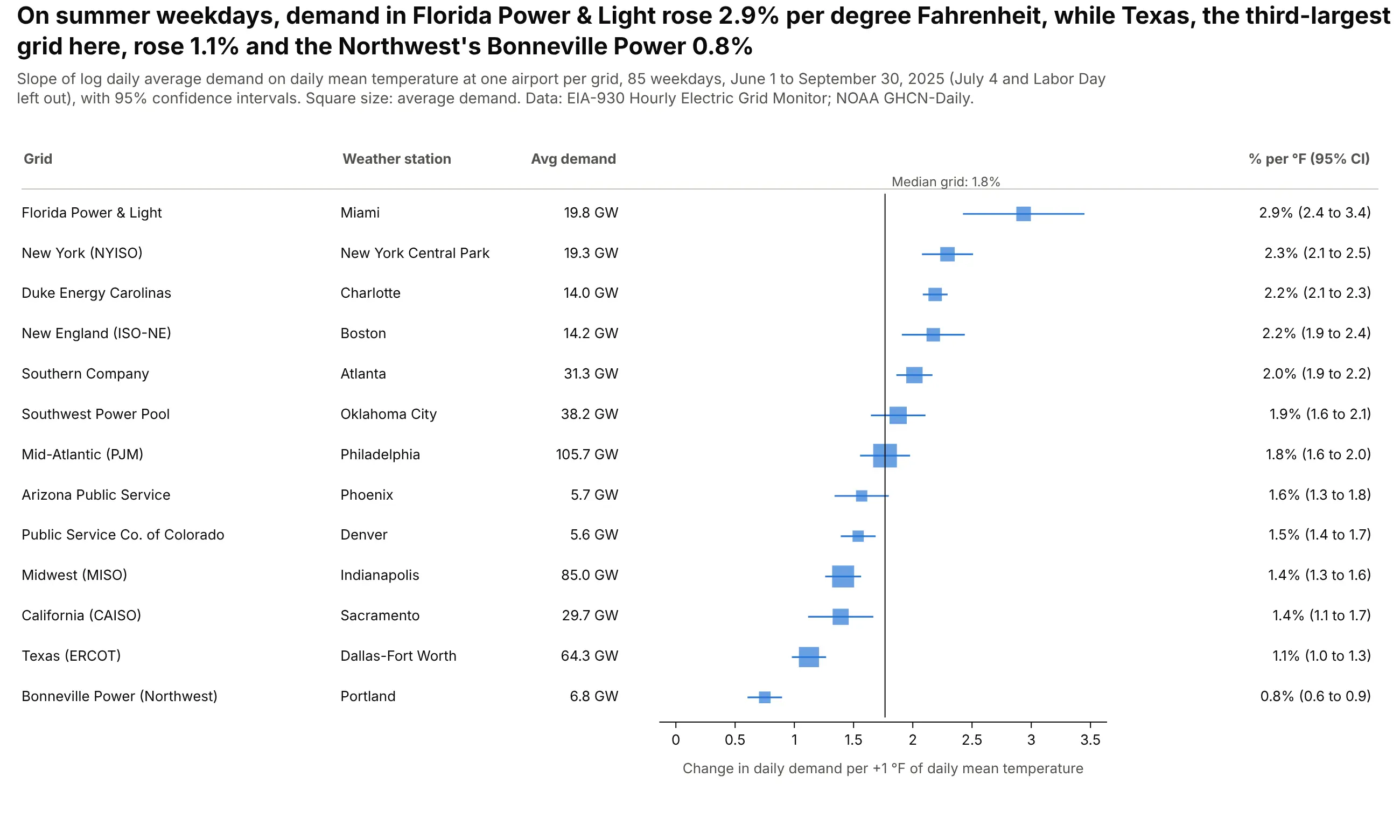
Forest plot of 13 US grids' summer weekday demand sensitivity to temperature, from Florida Power & Light at 2.9% per degree Fahrenheit to Bonneville Power at 0.8%, with ERCOT at 1.1% and a reference line at the 1.8% median

On summer weekdays in 2025, Florida Power & Light's demand rose 2.9% per degree Fahrenheit, against 1.1% for Texas and a median of 1.8% across 13 grids. Each row is a regression slope from 85 days. Data: EIA-930 Hourly Electric Grid Monitor and NOAA GHCN-Daily.

Tip: when there's no natural "no effect" value, draw the reference line at the median and say so.

Get the data from EIA-930 six-month BALANCE files (2025 Jan-Jun and Jul-Dec, adjusted demand) and
NOAA GHCN-Daily station CSVs (TMAX, TMIN) for one airport per grid
and shape it into a table (columns: ba, grid, station, date, demand_gw, tmean_f), June-September 2025.

For each grid, regress ln(demand_gw) on tmean_f over weekdays and convert the slope to % per °F
with a 95% CI. Build a plotly forest plot sorted by slope, squares sized by average demand,
a line at the median, and a table with the station and average GW.

8. An e-mail A/B test, by customer segment

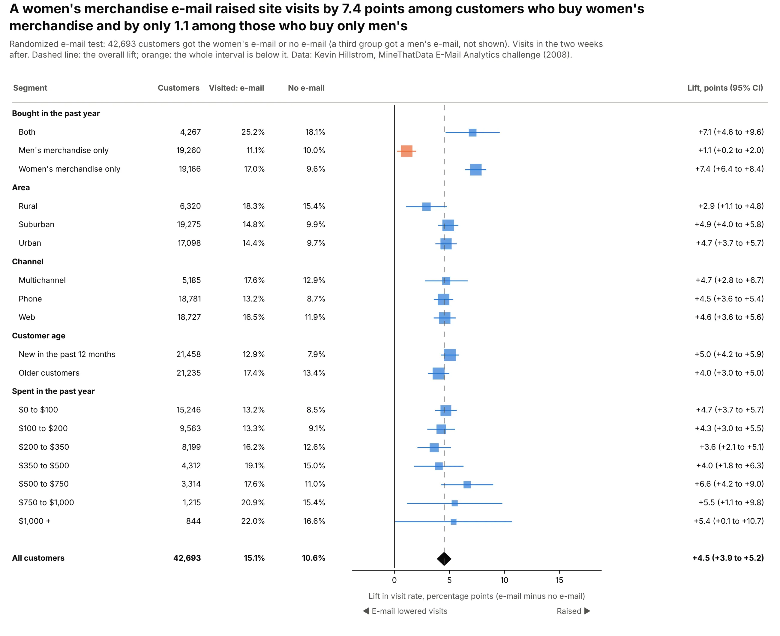
Forest plot of the lift in site visits from a women's merchandise e-mail in 18 customer segments, from +7.4 points for women's-only buyers to +1.1 for men's-only buyers in orange, with a dashed line at the overall +4.5

A women's merchandise e-mail raised visits by 4.5 points overall, by 7.4 among customers who buy women's merchandise and by only 1.1 among those who buy only men's. The other segments sit close to the overall lift. Data: Kevin Hillstrom, MineThatData E-Mail Analytics challenge (2008).

Tip: draw a dashed line at the overall effect, because the question for each segment is whether it differs from the average, not from zero.

Get the data from Kevin Hillstrom's MineThatData e-mail experiment CSV (64,000 customers randomly
sent a men's e-mail, a women's e-mail or none)
and shape it into a table (columns: segment, history_segment, mens, womens, zip_code, newbie, channel, visit).

Build a plotly forest plot of the visit-rate lift (women's e-mail minus no e-mail, percentage points)
with a 95% CI for each value of: past purchases, area, channel, new vs older, spend band.
Header row per variable, overall diamond, dashed line at the overall lift, line at 0.

9. Home advantage without crowds

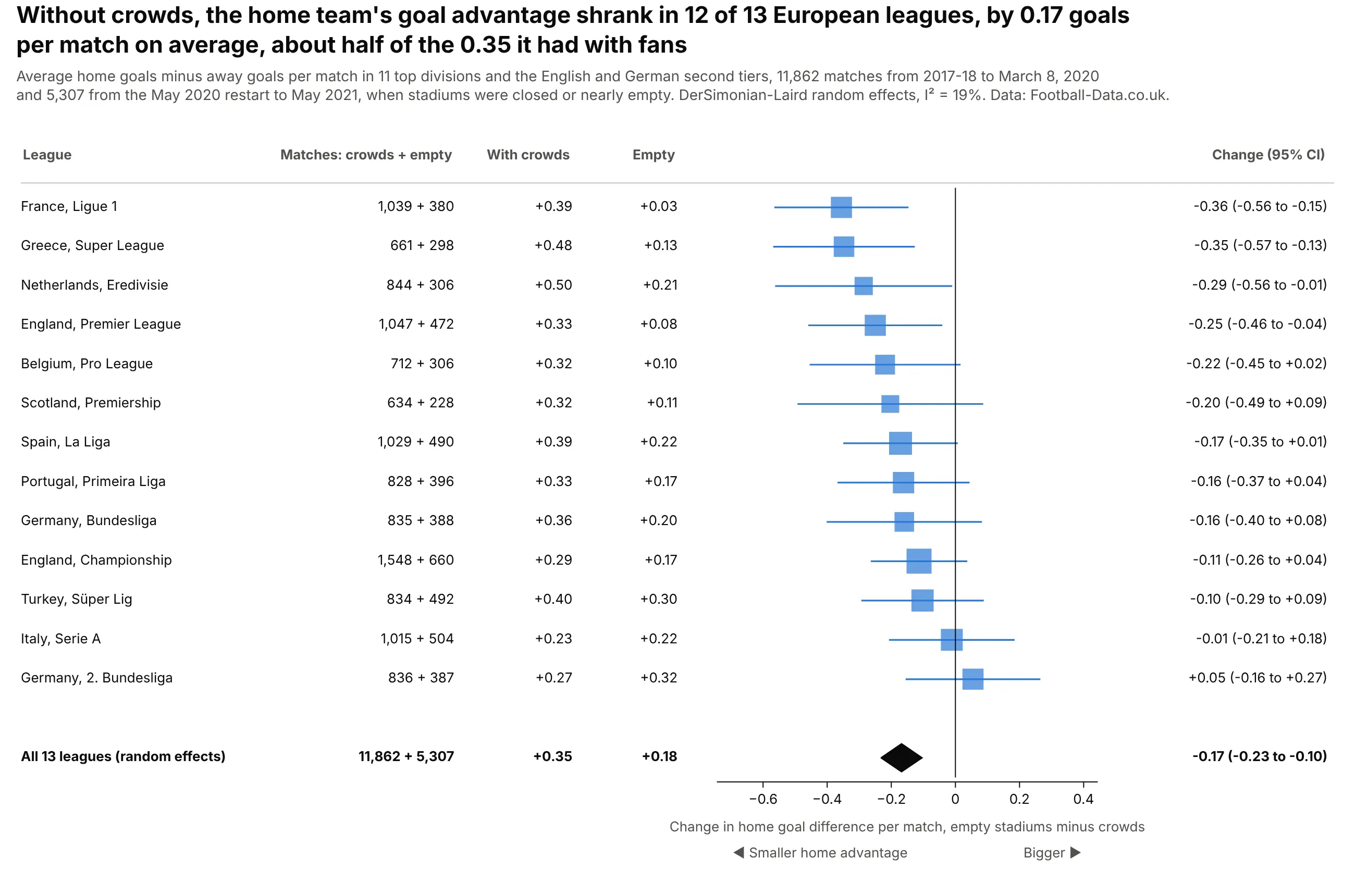
Forest plot of 13 European football leagues' change in home goal difference per match when stadiums were empty, from Ligue 1 at -0.36 to 2. Bundesliga at +0.05, with a random-effects diamond at -0.17 (-0.23 to -0.10)

When stadiums emptied in 2020-21, the home team's goal advantage shrank in 12 of 13 leagues, by 0.17 goals per match on average, about half of the 0.35 it had with fans. Pooling the leagues gives a far tighter answer than any one league. Data: Football-Data.co.uk.

Tip: treat each league as a study; a meta-analysis works on any set of comparable estimates, not only clinical trials.

Get the data from Football-Data.co.uk season CSVs (2017-18 to 2020-21) for E0, E1, D1, D2, SP1, I1,
F1, N1, P1, T1, B1, SC0 and G1
and shape it into a table (columns: league, season, date, home, away, home_goals, away_goals).

For each league, compare home minus away goals per match before March 9, 2020 and from May 16, 2020
(difference of means, 95% CI). Build a plotly forest plot sorted by the change, line at 0,
DerSimonian-Laird diamond, table with matches and the two averages.