Error Bars - A Complete Guide

TL;DR

• Error bars are the lines drawn above and below (or either side of) a value to show how uncertain it is or how spread out the data behind it are. A bar can show a standard deviation, a standard error or a 95% confidence interval, and for the same data those can differ several-fold, so a chart must say which one it uses.
• Charts with error bars are also known as interval plots and dot-and-whisker plots, the continuous version is an error band, and they are similar to forest plots, box plots and dot plots.
• Use 95% confidence intervals to compare estimates, standard deviations to show how much individuals vary, and a shaded error band when the x axis is continuous, like a time series.
• You can add error bars to any Plotly scatter, line or bar chart with error_y (or error_x), and asymmetric error bars with arrayminus; an error band is two lines with fill="tonexty".

What are error bars?

Error bars look like this:

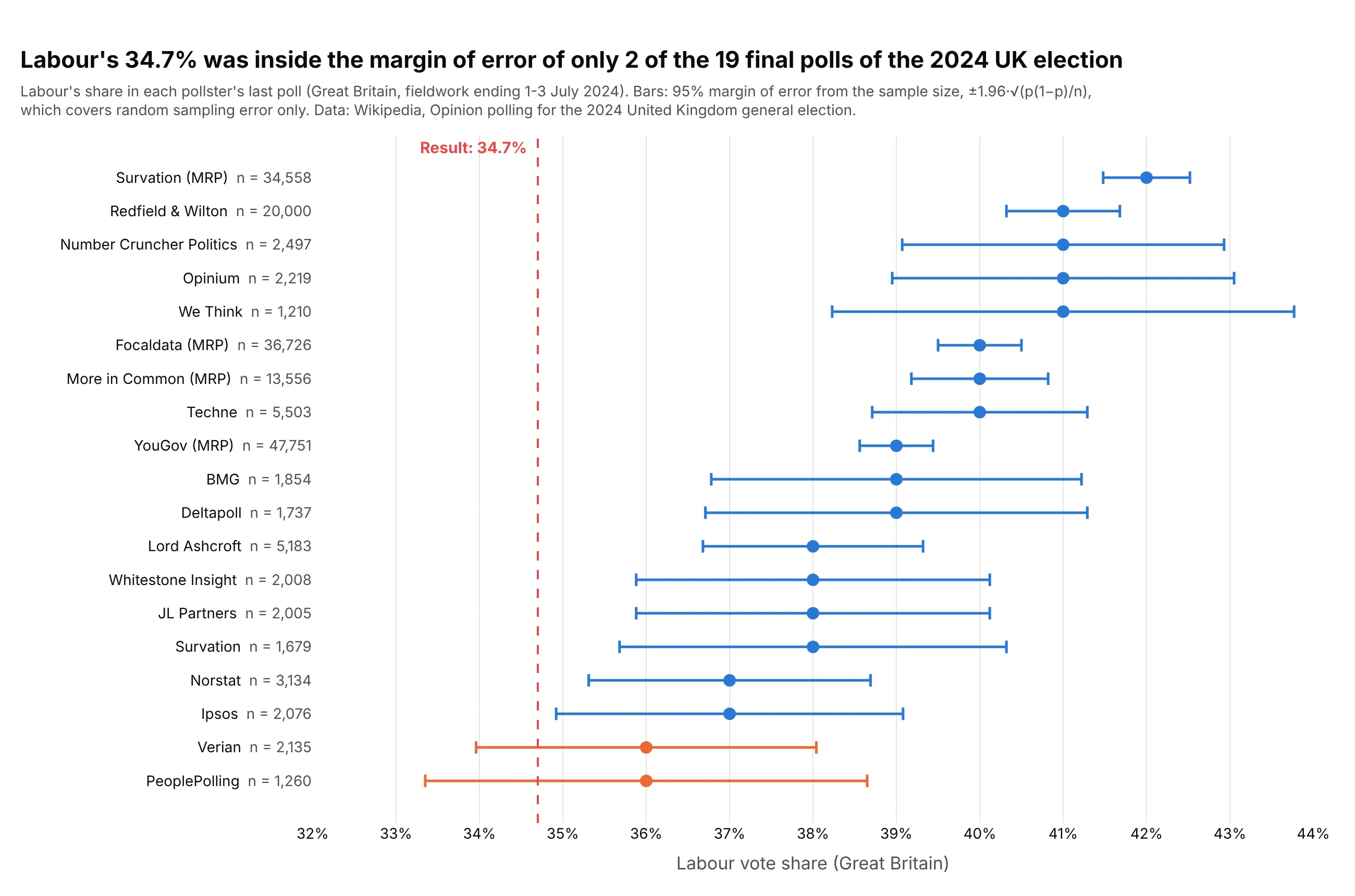
Data: Wikipedia, Opinion polling for the 2024 United Kingdom general election.

How do you read error bars? In the example above, notice these things:

• Each dot is one pollster's last estimate of Labour's vote share in Great Britain, and its bar is the 95% margin of error that its sample size alone implies. The subtitle says so, because a bar on its own doesn't tell you what it measures.
• Bars get shorter as samples get bigger. We Think asked 1,210 people and its margin is ±2.8 points; YouGov's MRP model used 47,751 respondents, about 40 times as many, and its bar is about a sixth as long.
• The result, 34.7%, sits inside the bars of only 2 of the 19 polls. Every poll had Labour higher, at 39.0% on average.
• A short bar is not a correct estimate. YouGov's MRP interval runs from 38.6% to 39.4%, nowhere near the result, because a margin of error covers random sampling error and nothing else.

It's often used for charts like these:

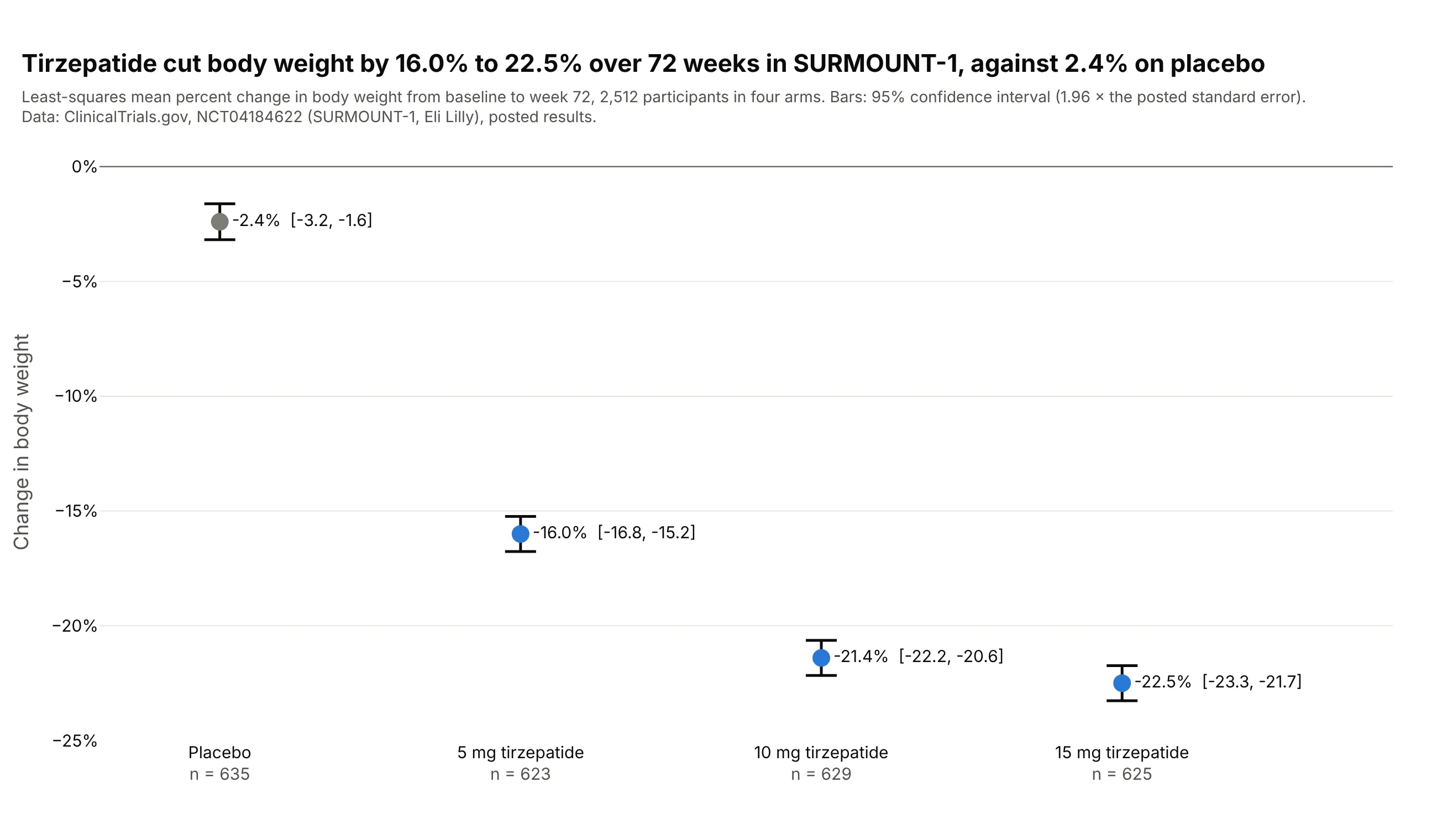
Clinical trial results. In SURMOUNT-1, tirzepatide cut body weight by 16.0% to 22.5% over 72 weeks against 2.4% on placebo, and the 95% intervals of the 10 mg and 15 mg arms overlap. Many trials side by side become a forest plot. Data: ClinicalTrials.gov, NCT04184622.

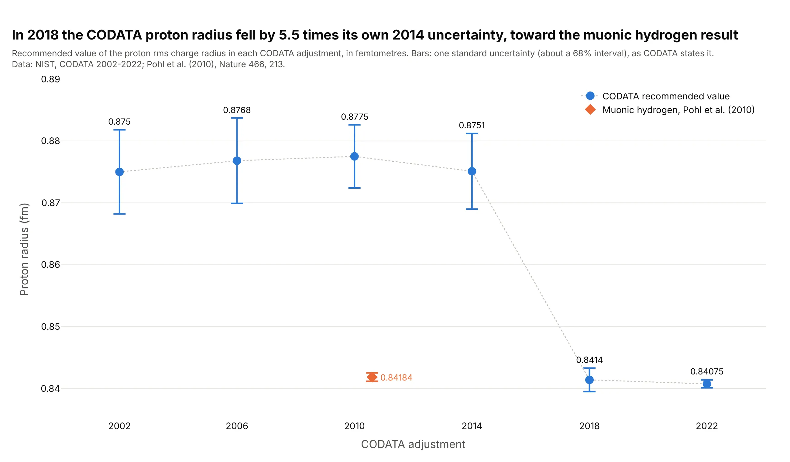
Physical constants. The CODATA value of the proton radius dropped by 5.5 times its own 2014 uncertainty in 2018, after muonic hydrogen measurements gave a smaller radius. Data: NIST CODATA 2002-2022; Pohl et al. (2010).

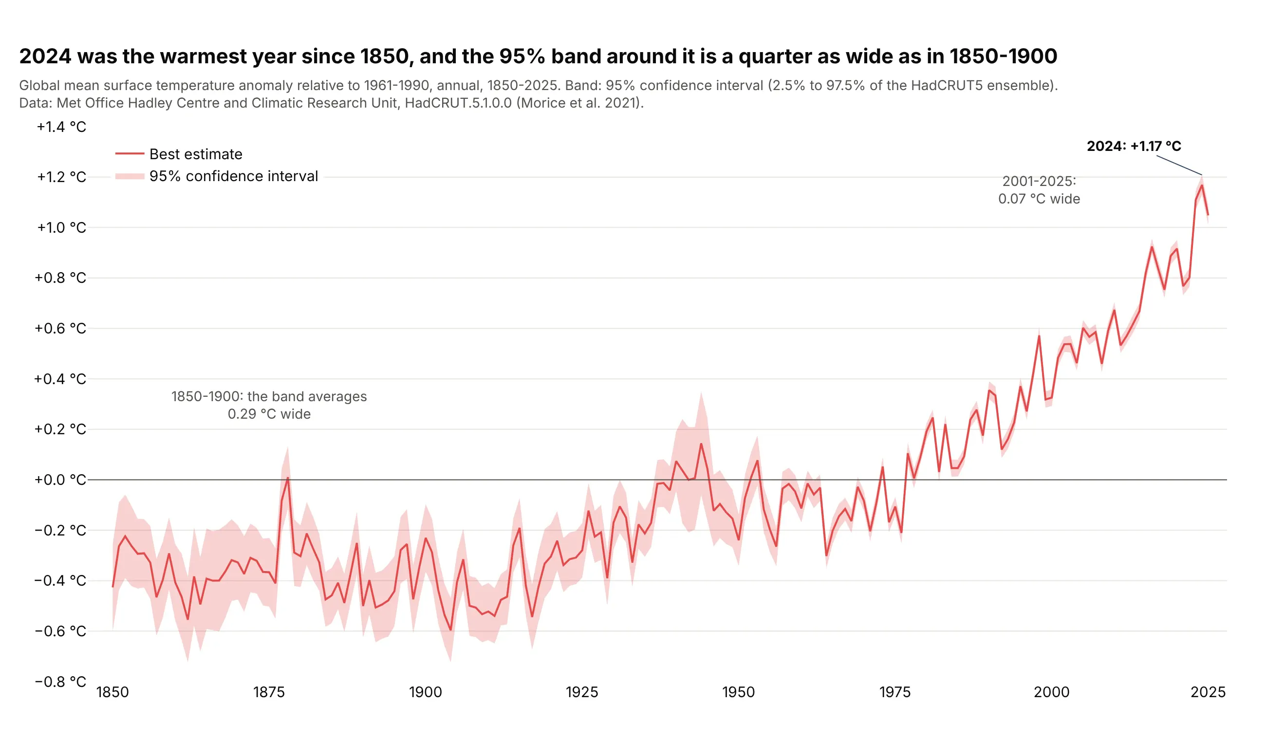
Climate records. 2024 was the warmest year in the HadCRUT5 record, and the 95% band around global temperature is about a quarter as wide now as in 1850-1900, when there were far fewer measurements. Data: Met Office Hadley Centre and CRU, HadCRUT5 (Morice et al. 2021).

A short history

Error bars draw quantities that statistics gave names to over the 20th century. Student's 1908 paper "The Probable Error of a Mean" showed how to judge a mean from a small sample, and Jerzy Neyman's 1937 theory of confidence intervals defined the 95% interval most bars show today. The confusion between the kinds of bars is just as old: Brown (1982) reviewed the misuse of standard deviation and standard error in medical journals, and when Belia et al. (2005) asked 473 authors in psychology, neuroscience and medicine to move two error bars until the means were just significantly different, many "do not adequately distinguish CIs and SE bars". The first of Cumming, Fidler and Vaux's (2007) eight rules for error bars is "always describe in the figure legends what they are".

Alternatives to error bars

Here's the same guinea pig experiment drawn six ways. Some are better for the question, some worse, some just different:

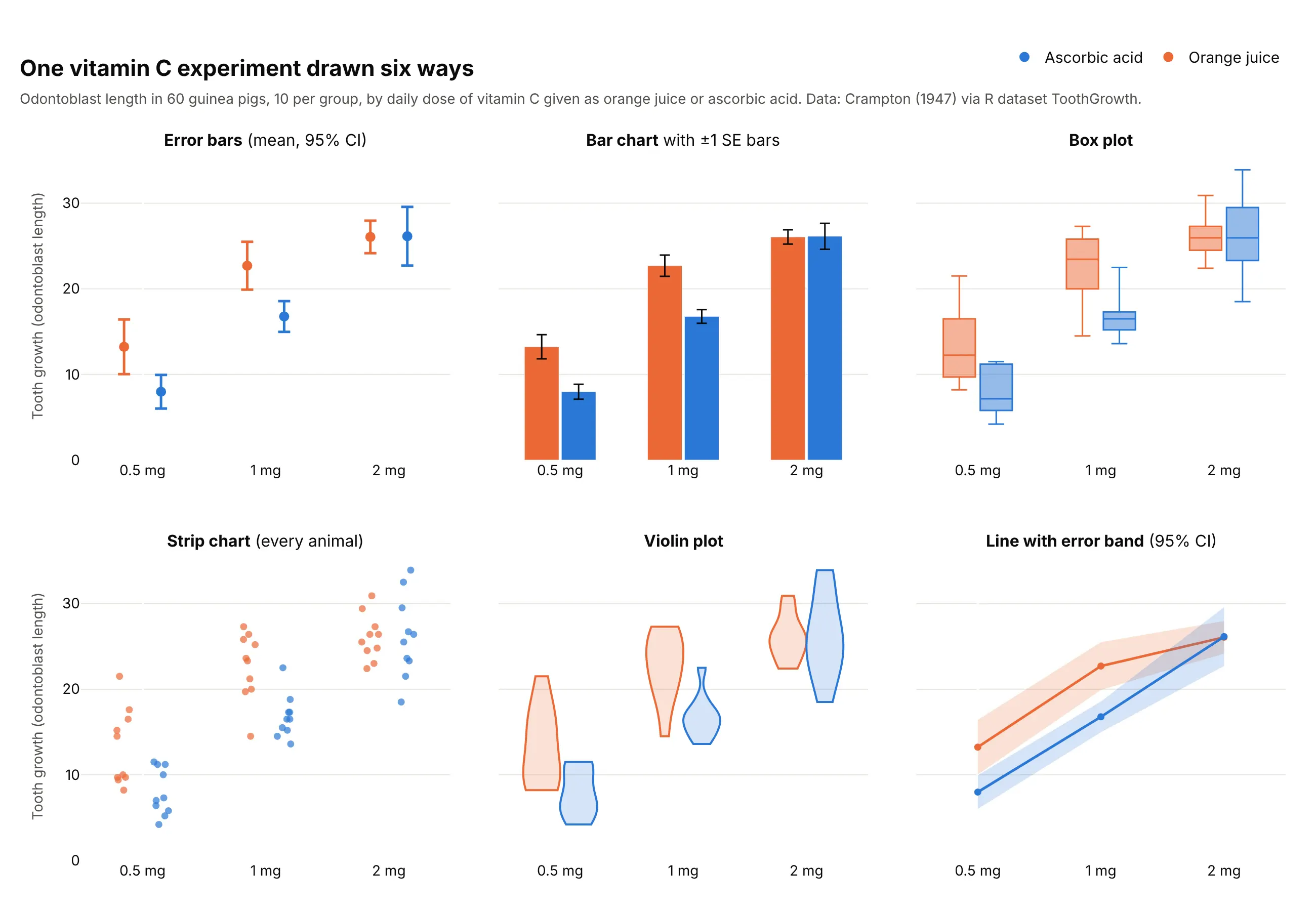
• Bar chart with error bars (worse for means). The bars fill the space from zero, which draws the eye to the area instead of the mean, and these standard error bars are about half as long as 95% intervals, so the groups look more different than they are. Bars from zero are fine for amounts that start at zero, as in the CO2 example below.
• Box plot (different). It shows the spread of the animals (median, quartiles, range) instead of the uncertainty of the mean, which is a different question.
• Strip chart (better for small groups). With 10 animals per group you can show every one, and Cumming et al. recommend plotting the individual points when n is very small. Add a mean and interval on top for the best of both.
• Violin plot (worse here). Ten points are too few for a smooth shape, so the outlines mostly show where the extremes happen to be.
• Line with error band (works too, for ordered x). When x is a dose, a time or another number, a shaded band between the lower and upper limits reads better than a row of bars, and it is how the temperature chart above is drawn.

How to make error bars

With AI

ChatGPT, Claude Code, GitHub Copilot, Cursor and other AI tools are excellent at writing Plotly code. Name Plotly in the prompt, and say what the bars should show, so the code computes the right thing:

With Plotly Studio

Plotly Studio is a desktop app where you point an AI at a dataset and it builds charts and a Dash app around your questions. Ask for error bars the same way:

Show the average monthly stock market return for each calendar month as dots with 95% confidence interval error bars, a line at zero, and the overall average as a dotted line.

Make error bars in Python or JavaScript

This is the code AI tools write under the hood. Plotly error bars come from one argument: in Plotly Express, error_x or error_y names the column with the bar length, and error_x_minus or error_y_minus makes them asymmetric. The Plotly error bars documentation has more:

An error band is two invisible lines with the space between them filled. Draw the lower limit first, then the upper one with fill="tonexty", as in the continuous error bands documentation:

To make a JavaScript error bars chart, give a plotly.js trace the same error_y object:

Plotly draws the bars; it doesn't compute them. Work out the standard deviation, standard error or interval first (pandas, NumPy or SciPy in Python), and pass the half-widths.

Share it

Every Plotly chart has a Share chart button (the cloud icon in its toolbar) that uploads it to Plotly Cloud and gives you a link. Only you can see it until you change its visibility.

For a live app, put the chart in a Dash app and publish it with the Plotly Cloud CLI. Coding agents can run these commands for you:

If your data has to stay in your own cloud or data center, publish to Dash Enterprise instead.

Dos and don'ts

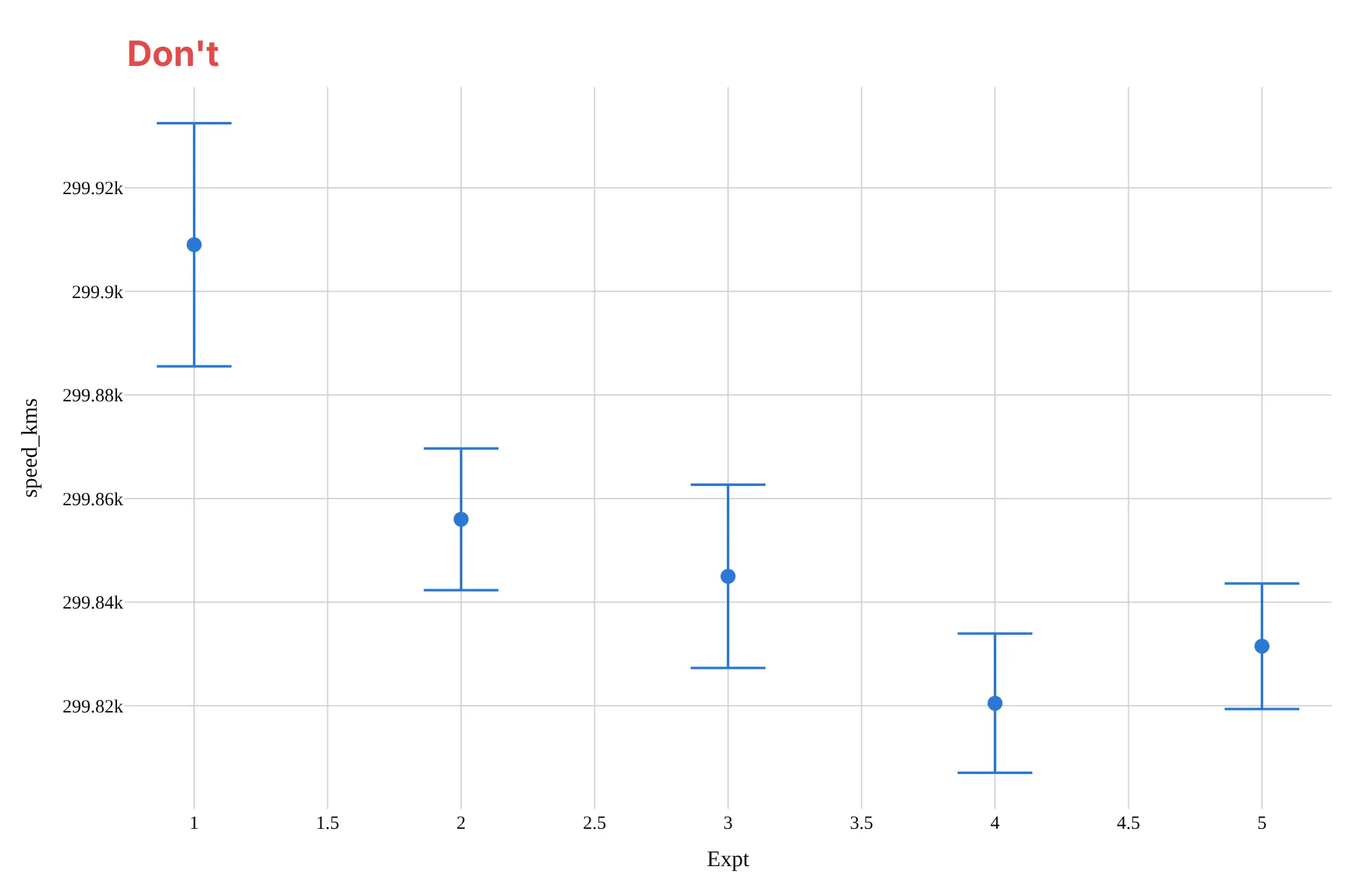
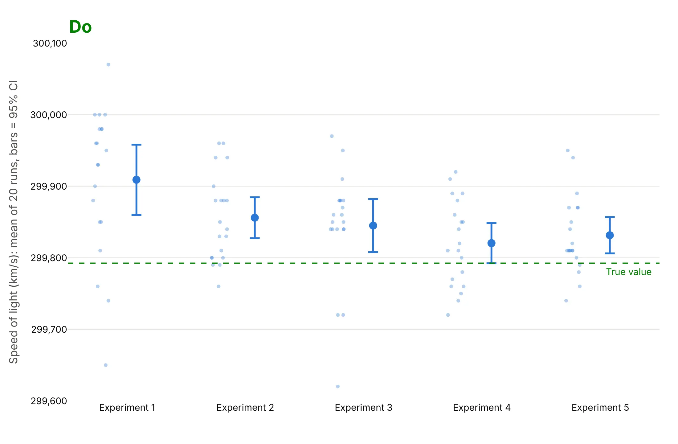
The most common mistake with error bars is not saying what they are. Here are Michelson's 1879 measurements of the speed of light, five experiments of 20 runs each, both ways, in the same color.

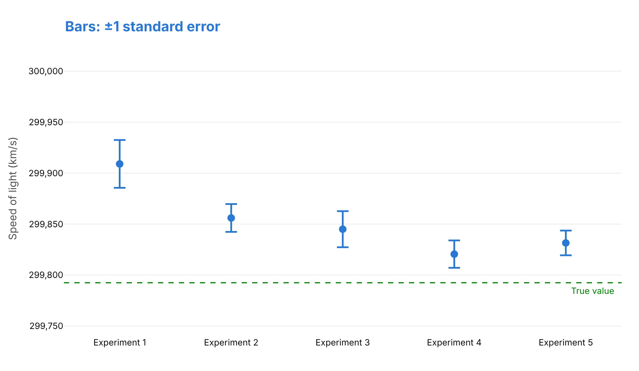
Don't draw bars without saying what they show (these are ±1 standard error, the shortest of the usual choices, so the experiments look more precise than they were), leave out the reference that gives them meaning, or use a default serif font, raw column names and ticks like "299.92k":

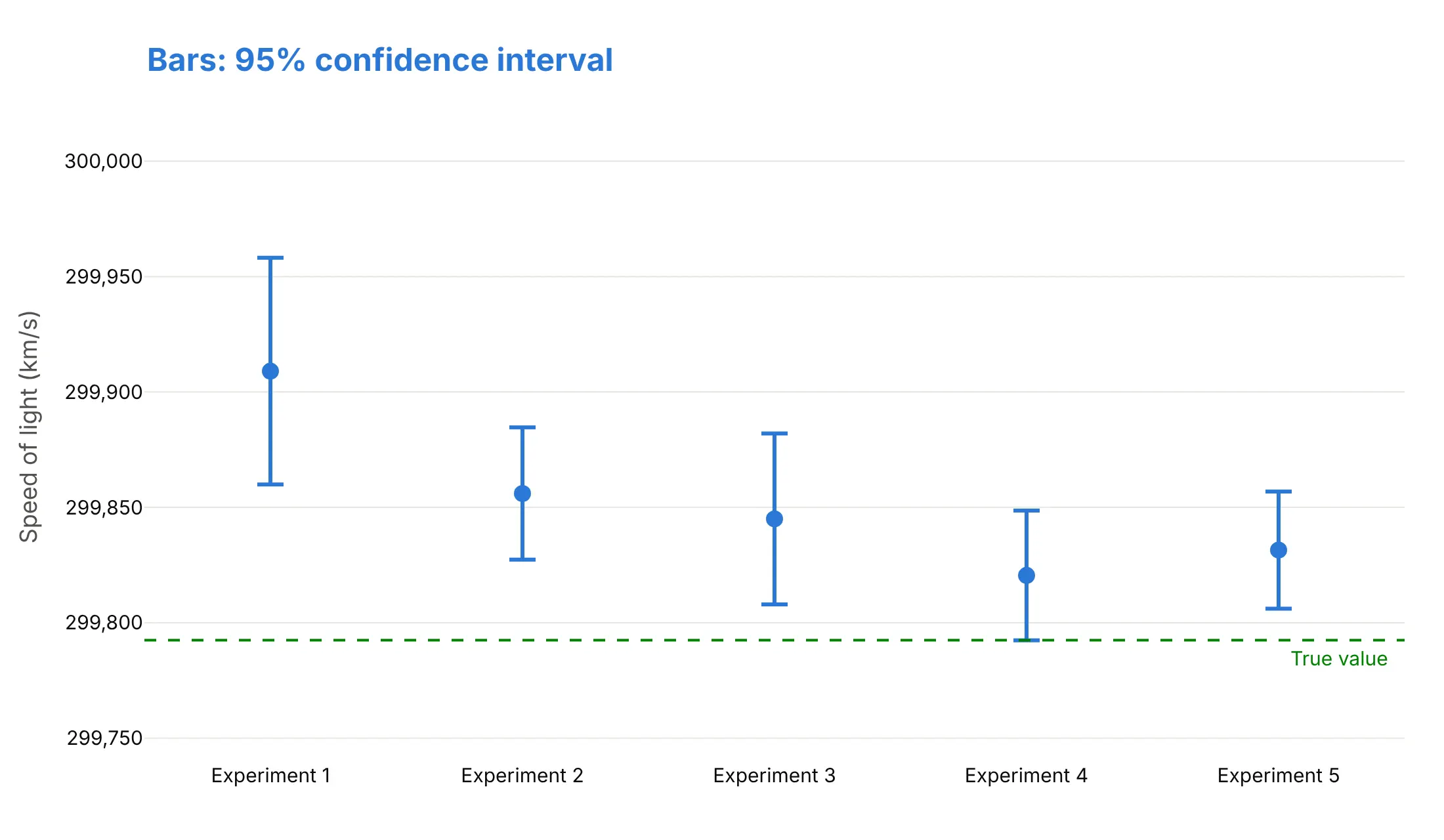
Do say what the bars are and how many values each mean comes from, show the runs behind the means when there are few of them, draw the true value, and format the axis:

What does the bar show?

The same five means with the three usual kinds of bar give three different answers to "was Michelson's apparatus biased?".

Standard deviation. It describes how spread out the 20 runs are and doesn't shrink with more runs. Three of the five bars reach the true value, which says single runs often landed near it.

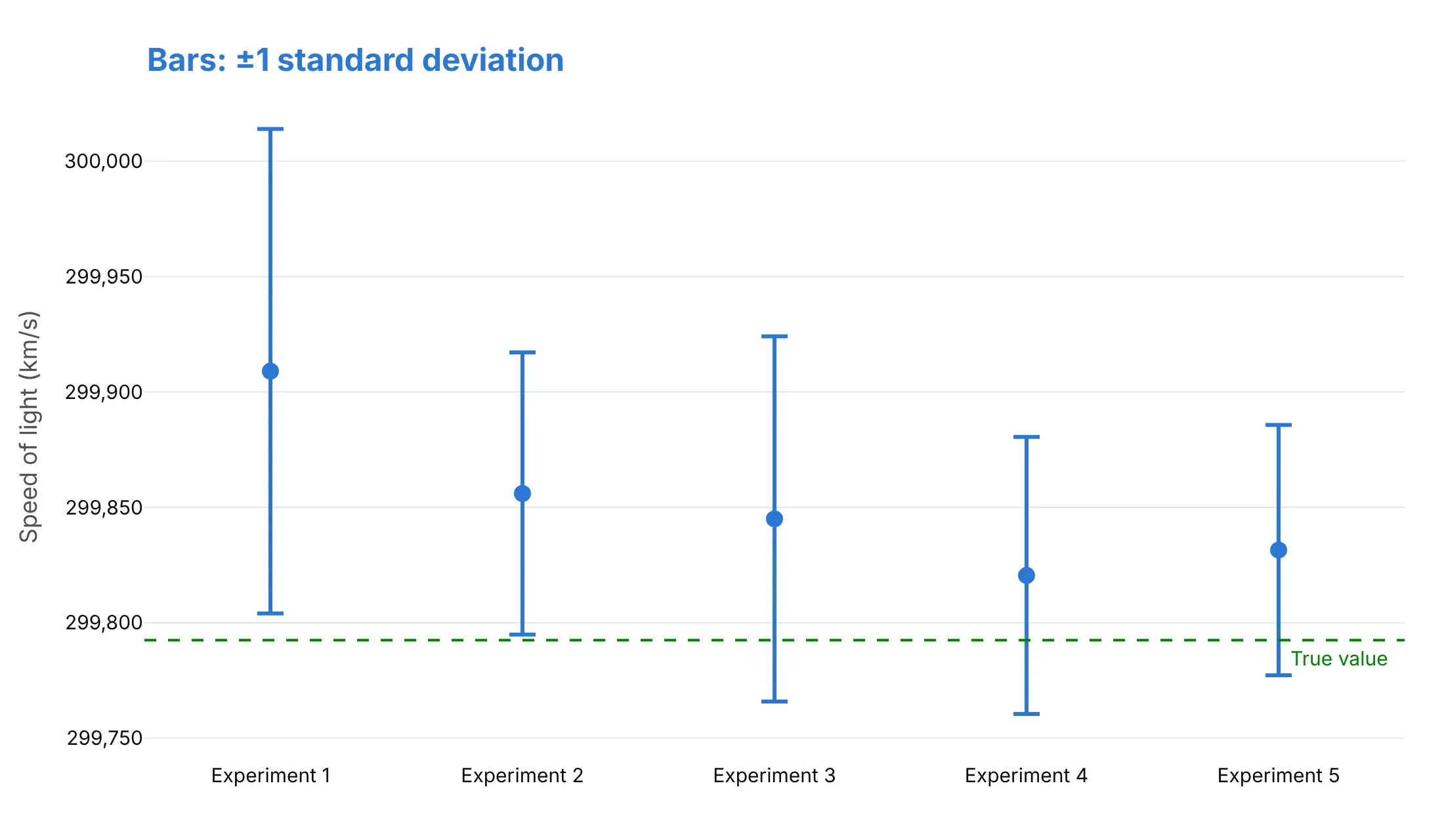
Standard error. It is the standard deviation divided by the square root of n (4.5 for 20 runs), and it measures how precisely the mean is known. None of the bars reaches the true value, but it is a 68% interval, not a 95% one.

95% confidence interval. It is the mean ± t × standard error, with t = 2.09 for 20 runs, so about twice the standard error. Only experiment 4's interval reaches the true value, just, so four of the five experiments were biased high. This is the bar to use when readers will compare means.

Checklist

Do

• Say in the subtitle, legend or axis title what the bars show (SD, SE or 95% CI) and the n behind each value.
• Use 95% confidence intervals when readers will compare groups, and standard deviations when they want to know how much individuals vary.
• Use a shaded error band for a continuous x axis, like a time series.
• Show the individual values when each group has only a few.
• Add the reference that matters: a true value, a result, a target or zero.
• Use asymmetric bars (arrayminus) when the interval isn't symmetric, and say whether a bar is uncertainty or spread.

Don't

• Leave the bars unexplained; in the Michelson example, ±1 SD bars are 4.5 times as long as ±1 SE bars.
• Read non-overlapping bars as "significant" without knowing what they are; for independent means with n of 10 or more, 95% CIs that overlap by half an arm still mean P ≈ 0.05 (Cumming et al. 2007).
• Treat a short bar as proof the estimate is right; it covers random error, not bias.
• Put means on bars from zero when zero isn't meaningful for the comparison.

Options to customize

Error bars in Plotly are an error_x or error_y object on a trace, and bands are filled scatter traces, so these are the options that matter most. The full lists are in the scatter trace reference and the Plotly Express reference.

1. px.scatter(..., error_y="col"), also in px.line and px.bar: the column with each bar's half-length; error_x for horizontal bars.
2. error_y_minus, error_x_minus (Plotly Express): a second column for the lower half, which makes the bars asymmetric.
3. error_y=dict(type="data", array=..., arrayminus=...) (graph objects): the bar lengths above and below each point; omit arrayminus for symmetric bars.
4. type="percent", "constant" or "sqrt" with value and valueminus: bars as a percentage of the value, one fixed length (the payroll example's ±122,000) or the square root of the value (Poisson counts).
5. thickness, width, color: line width, cap width (0 removes the caps) and color of the bars.
6. visible: turns a trace's bars on and off, for example from a button.
7. error_z on go.Scatter3d: bars in the third dimension.
8. fill="tonexty" with fillcolor: fills from this trace to the one before it, for error bands; use a transparent rgba color so the line shows through.
9. customdata and hovertemplate: put the interval's ends or the n in the hover text.
10. go.Scattergl: WebGL traces also take error_x and error_y, for tens of thousands of points.

More error bar examples

Six more charts with error bars built from real public data, each with its source, the technique that makes it work and a prompt to rebuild it.

1. Wind and solar output on the Texas grid

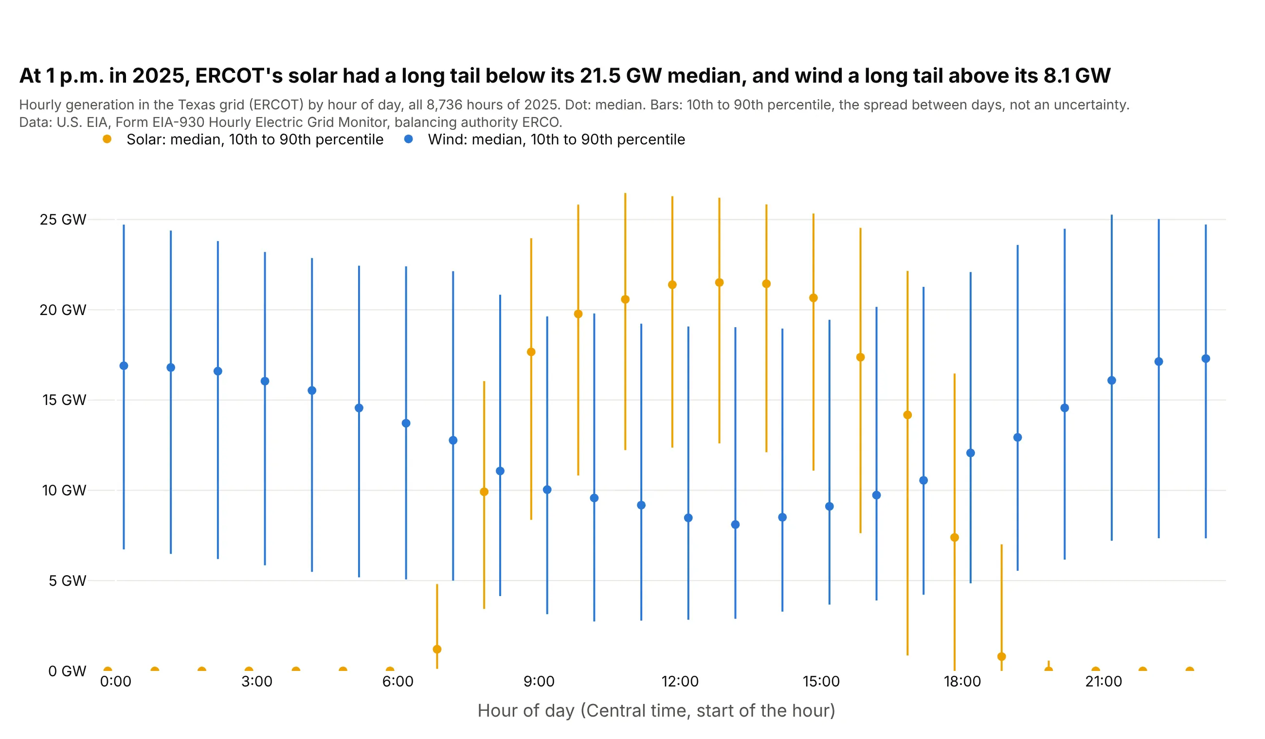
At 1 p.m. in 2025, ERCOT's median solar output was 21.5 GW, but on 1 day in 10 it was below 12.6 GW, while wind's median was 8.1 GW with 1 day in 10 above 19.0 GW. These bars show spread between days, not uncertainty, and the spread is lopsided. Data: U.S. EIA, Form EIA-930 Hourly Electric Grid Monitor.

Tip: for asymmetric error bars, pass the distance above the point as array and below it as arrayminus.

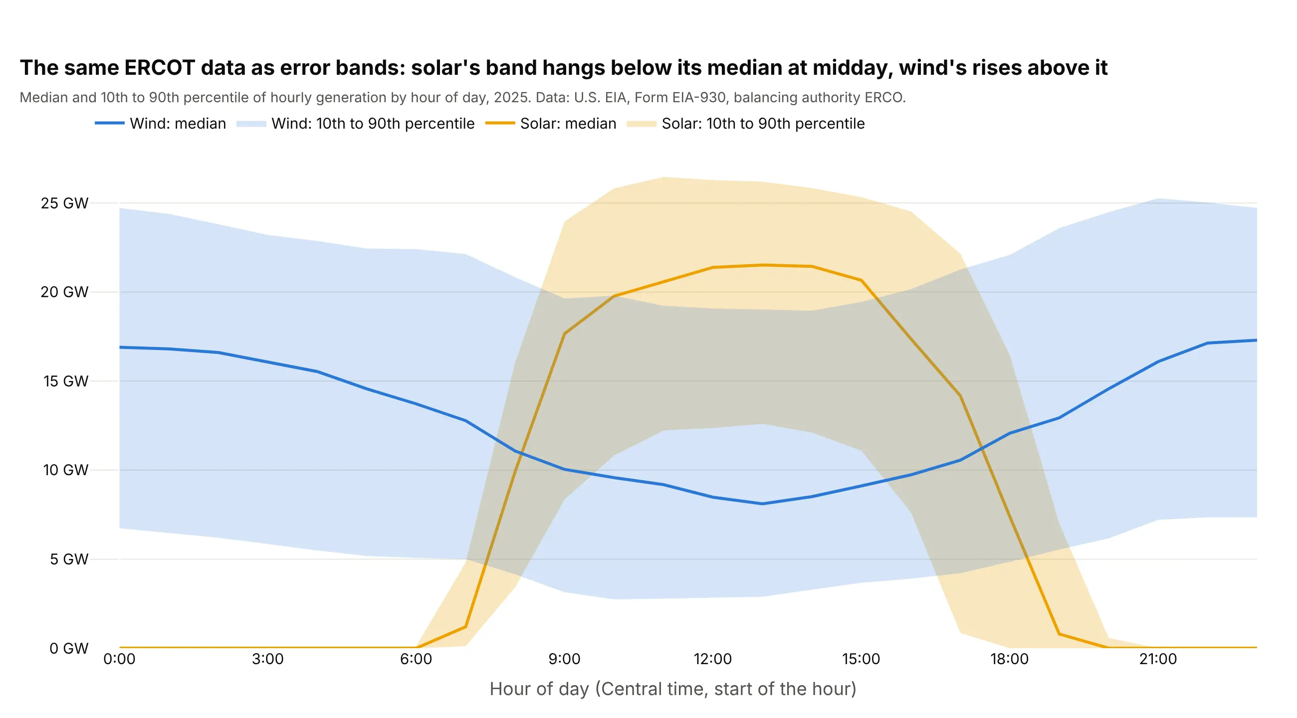
Another way to see it: the same percentiles as shaded error bands show the daily shapes at once, which works better when you have a value for every hour.

2. US job growth and the BLS margin of error

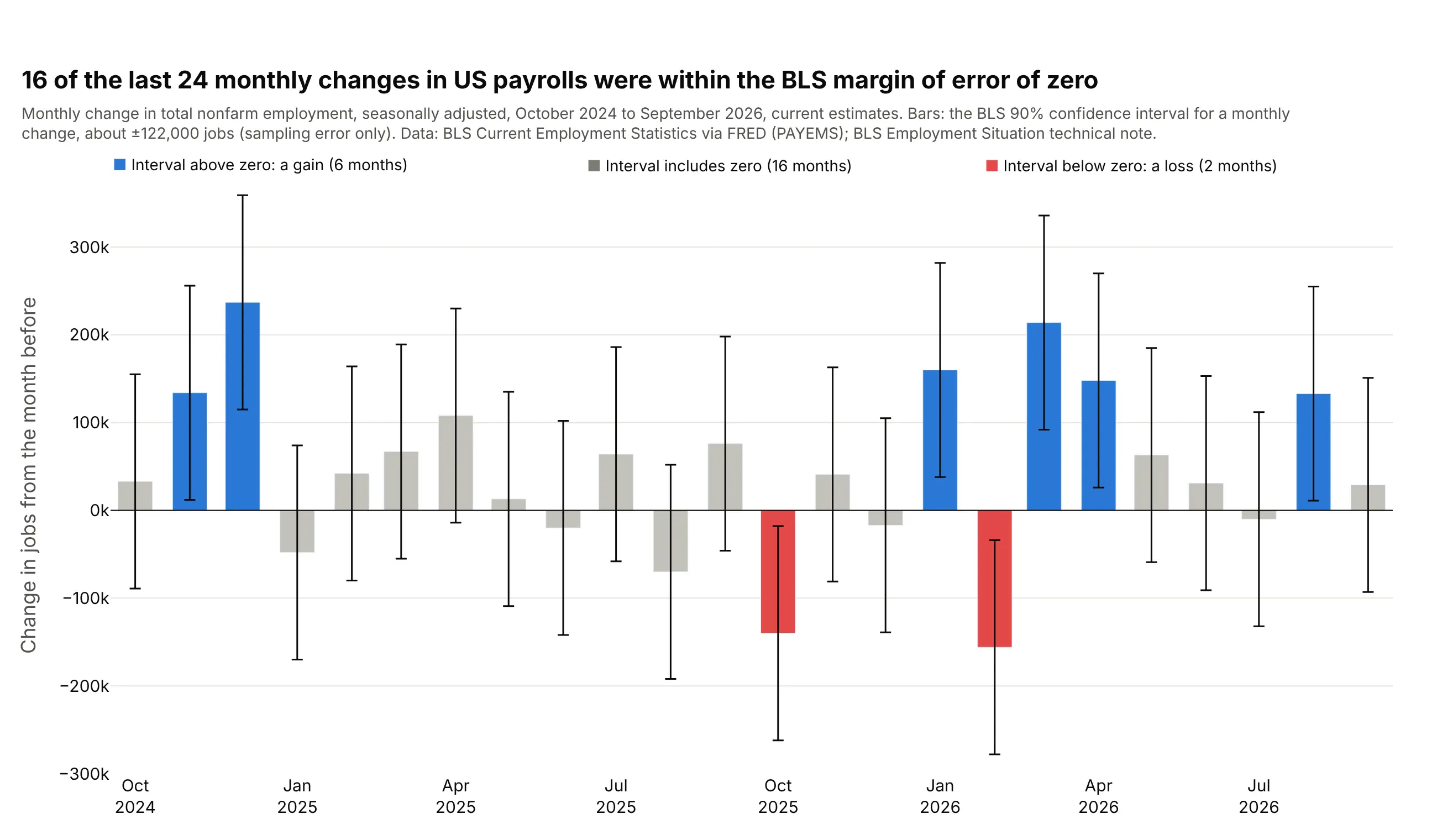
BLS says the 90% confidence interval for a monthly change in payrolls is about ±122,000 jobs, so 16 of the last 24 monthly changes can't be told apart from zero. Only 6 months were clearly gains and 2 clearly losses. Data: BLS Current Employment Statistics via FRED (PAYEMS); BLS Employment Situation technical note.

Tip: when every value has the same margin, error_y=dict(type="constant", value=122) draws it in one line.

3. Stock returns by calendar month

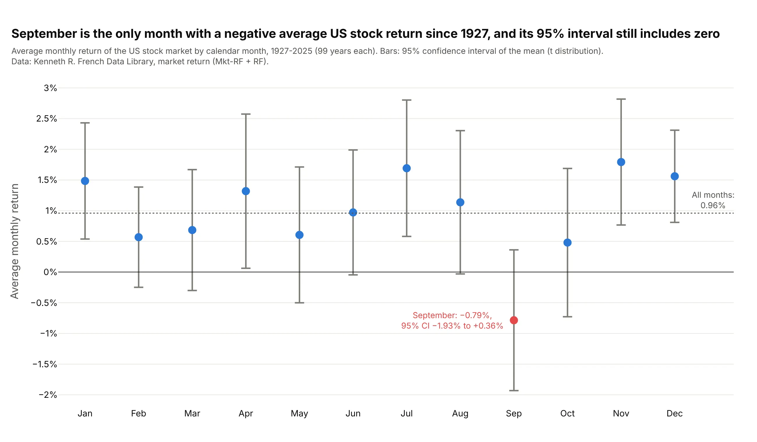
Since 1927, September is the only calendar month with a negative average US stock return, -0.79%, and its 95% interval still reaches +0.36%. Each month has 99 observations of a return with a standard deviation near 5%, which is why the intervals are about 2 points wide. Data: Kenneth R. French Data Library.

Tip: with 12 groups, one or two intervals can look unusual by chance alone, so draw the overall average as a reference and don't read much into a single month.

4. A pharmacokinetic profile, mean ± SD

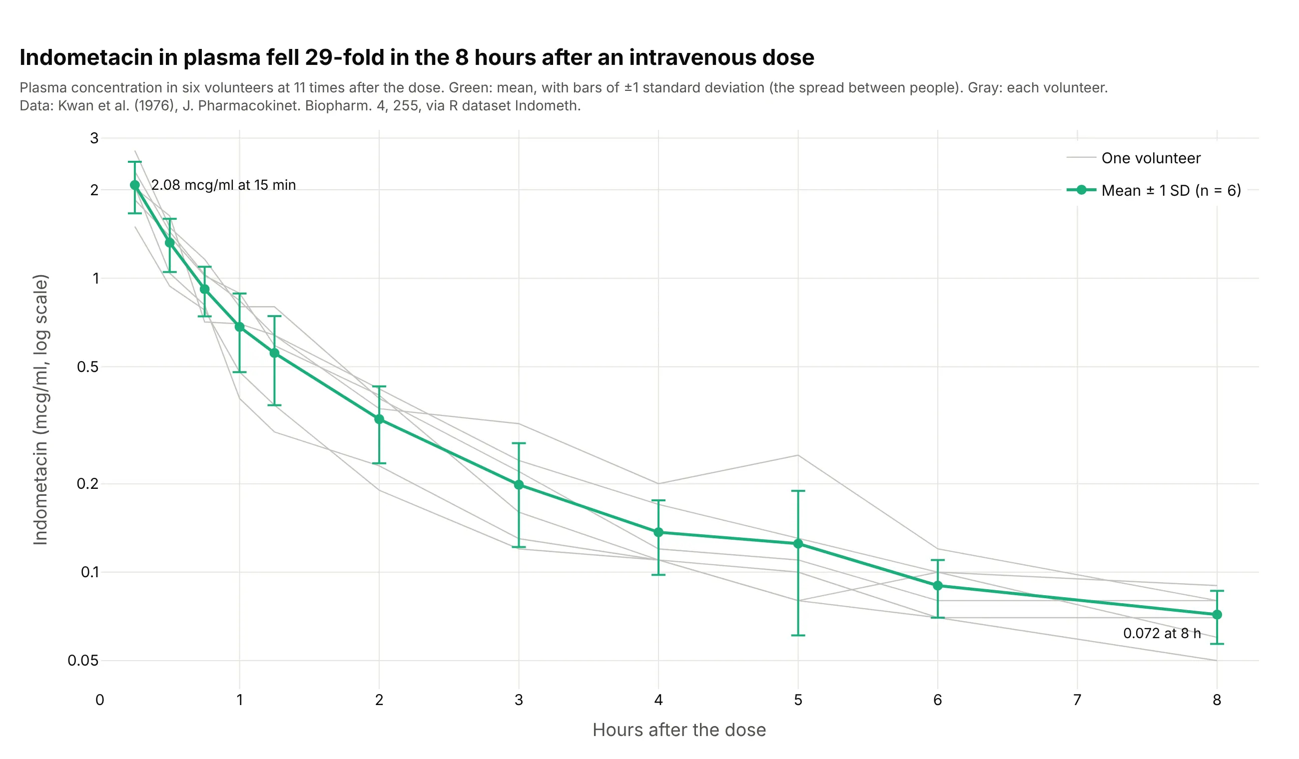
Indometacin in plasma fell 29-fold in the 8 hours after an intravenous dose in six volunteers. Pharmacokinetic tables usually report mean ± SD, so these bars show how much the people differ, and the gray lines show the same thing person by person. Data: Kwan et al. (1976) via R dataset Indometh.

Tip: on a log axis, ±SD bars look longer below the mean than above it, so say so or plot the individuals behind them.

5. Error bars in both directions: the TRAPPIST-1 planets

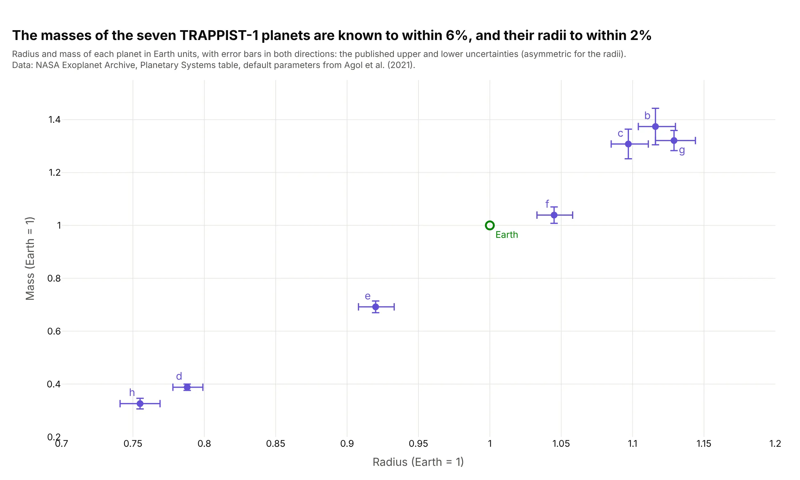
Transit timing pinned down the masses of all seven TRAPPIST-1 planets to within 6% and their radii to within 2%. Both coordinates are measurements, so each point needs a horizontal and a vertical bar, and the radius bars are slightly asymmetric. Data: NASA Exoplanet Archive, default parameters from Agol et al. (2021).

Tip: pass both error_x and error_y, each with array and arrayminus, to draw the published upper and lower uncertainties.

6. The record rise in atmospheric CO2

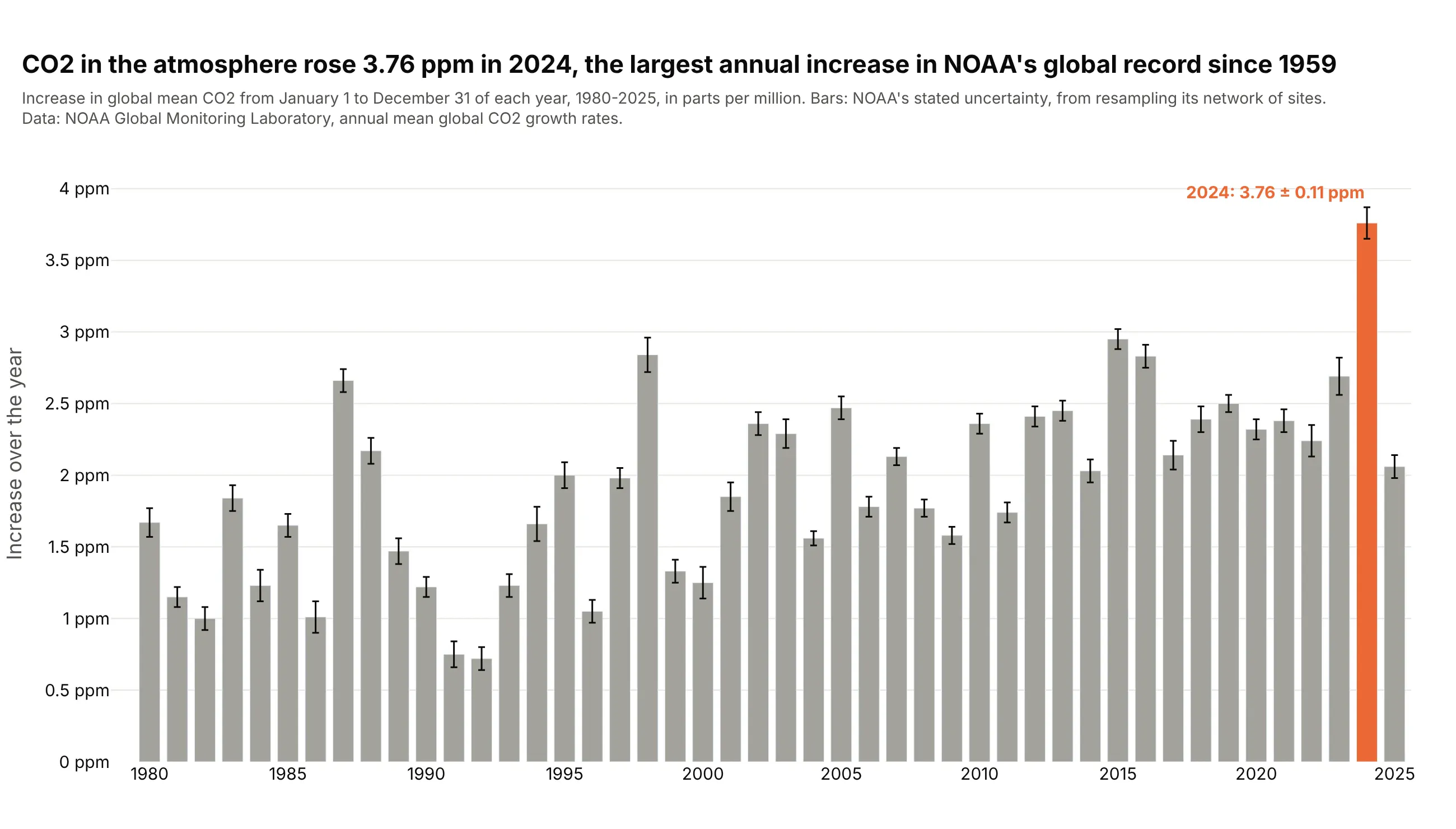
CO2 in the atmosphere rose 3.76 ± 0.11 ppm in 2024, the largest annual increase in NOAA's global record since 1959. The bottom of 2024's bar, 3.65 ppm, is above the top of every other year's. Data: NOAA Global Monitoring Laboratory.

Tip: error bars on bars are honest when the bar is an amount that starts at zero, and when the source doesn't state a confidence level, write "stated uncertainty".