Box Plots - A Complete Guide

TL;DR

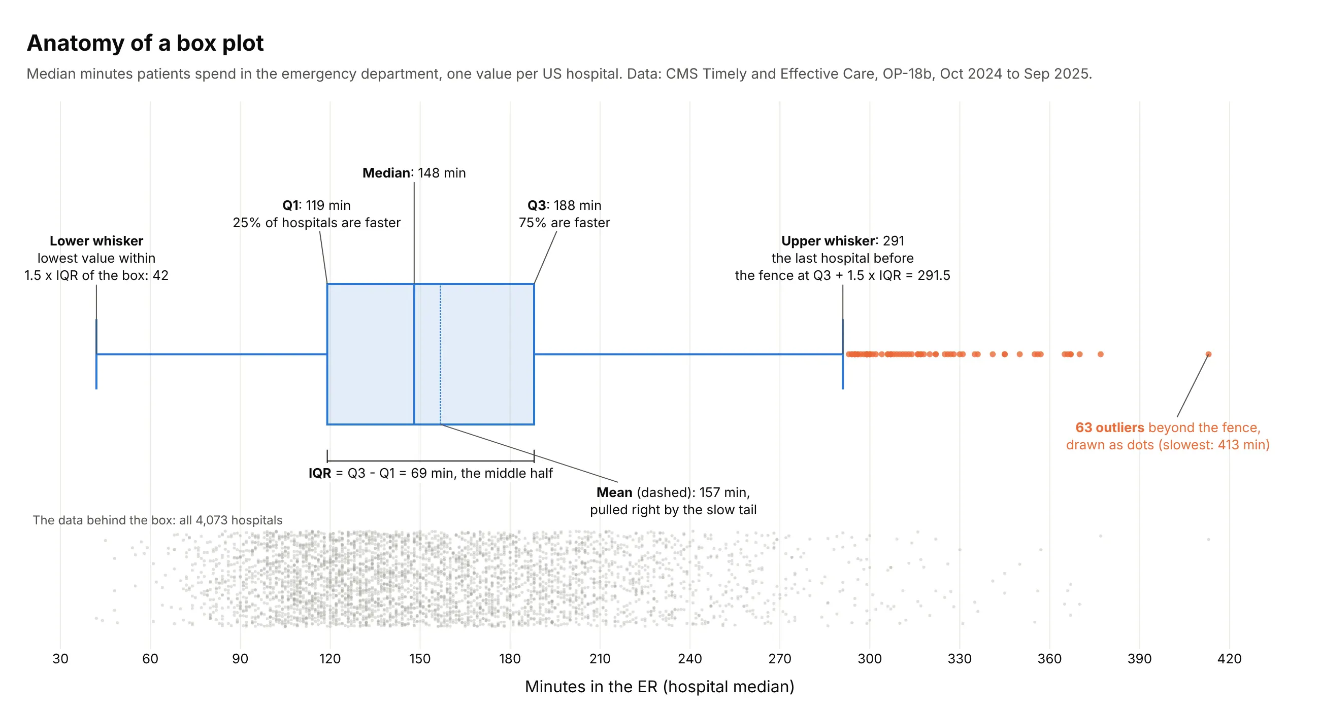
• A box plot summarizes a group of numbers with five values: a box from the first to the third quartile, a line at the median, and whiskers to the furthest points within 1.5 times the box's length, with anything beyond drawn as an outlier.
• Box plots are also known as box-and-whisker plots, box-and-whisker diagrams and boxplots, and are similar to violin plots, histograms and ridgeline plots.
• Use one to compare a number across many groups at once, such as 50 states, 49 industries or 20 drivers, where a histogram per group would no longer be readable.
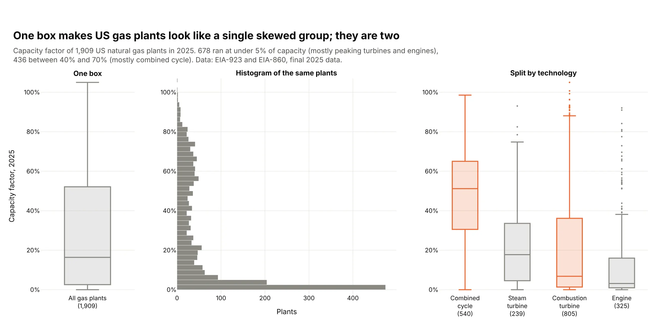
• A box hides the shape inside it, so two clusters or a tiny sample look like an ordinary box. Show the points or check a histogram before you publish.
• Any coding agent can make one with Plotly in a minute. In Python it's px.box(df, x="group", y="value").

What is a box plot?

Box plots look like this:

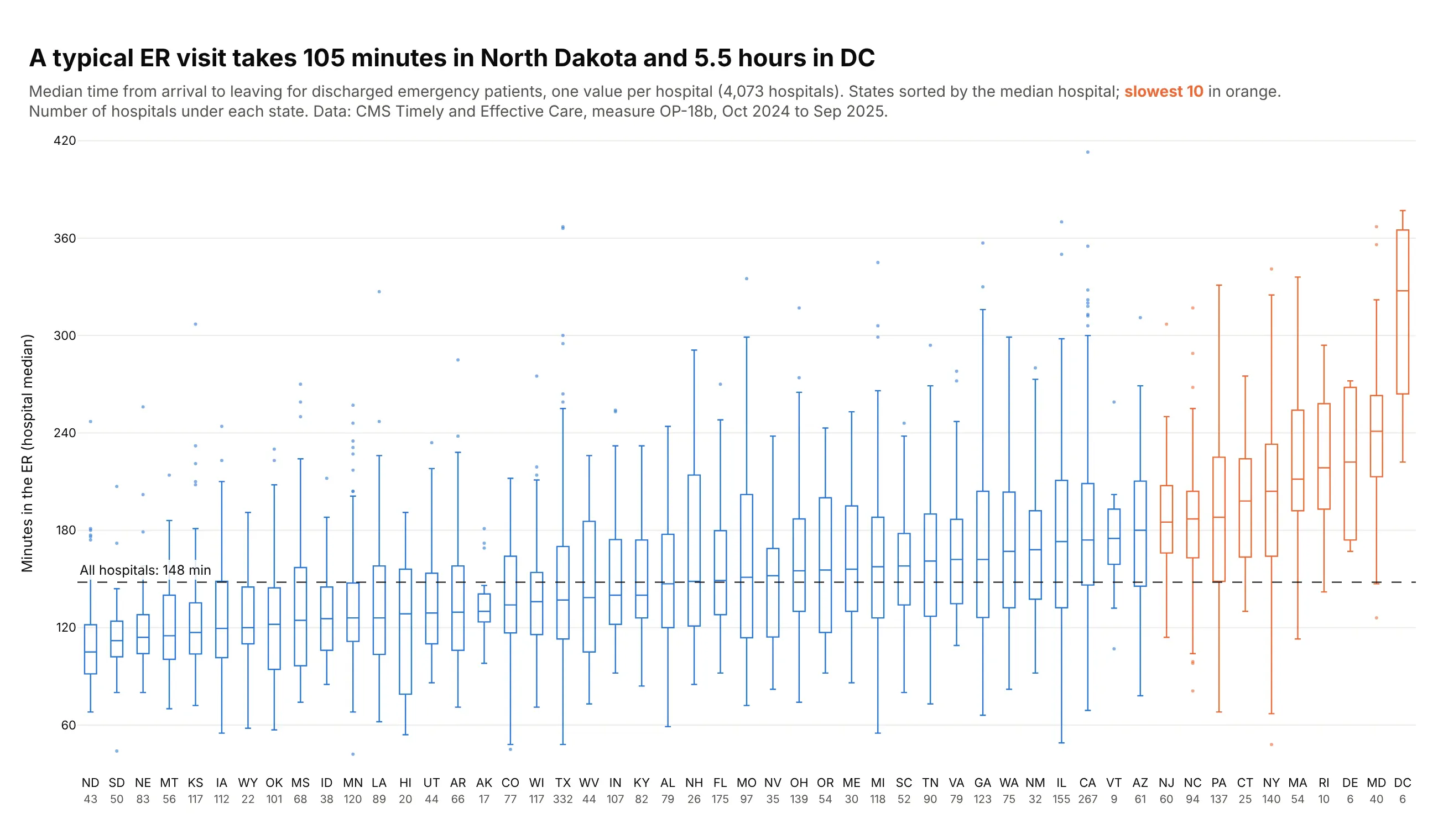
Data: CMS Timely and Effective Care, measure OP-18b, October 2024 to September 2025.

How do you read a box plot? In the example above, notice these things:

• Each box is one state, built from the median ER times of its hospitals, and the number of hospitals is printed under each state's name.
• The line inside a box is the state's median hospital, and the box covers the middle half of its hospitals, so North Dakota's box at the far left sits low and DC's at the far right sits high.
• The whiskers reach the furthest hospitals within 1.5 box lengths, and the dots beyond them are outliers, like Loma Linda University Medical Center in California, the slowest hospital in the chart.
• The states are sorted by their median and the dashed line marks the median of all hospitals, so you can see where states cross from faster than typical to slower, and the orange boxes for the 10 slowest states are mostly in the Northeast and Mid-Atlantic.
• Check the counts before trusting a box, because DC's tall box comes from only 6 hospitals, which is far less data than a box like Texas's.

It's often used for charts like these:

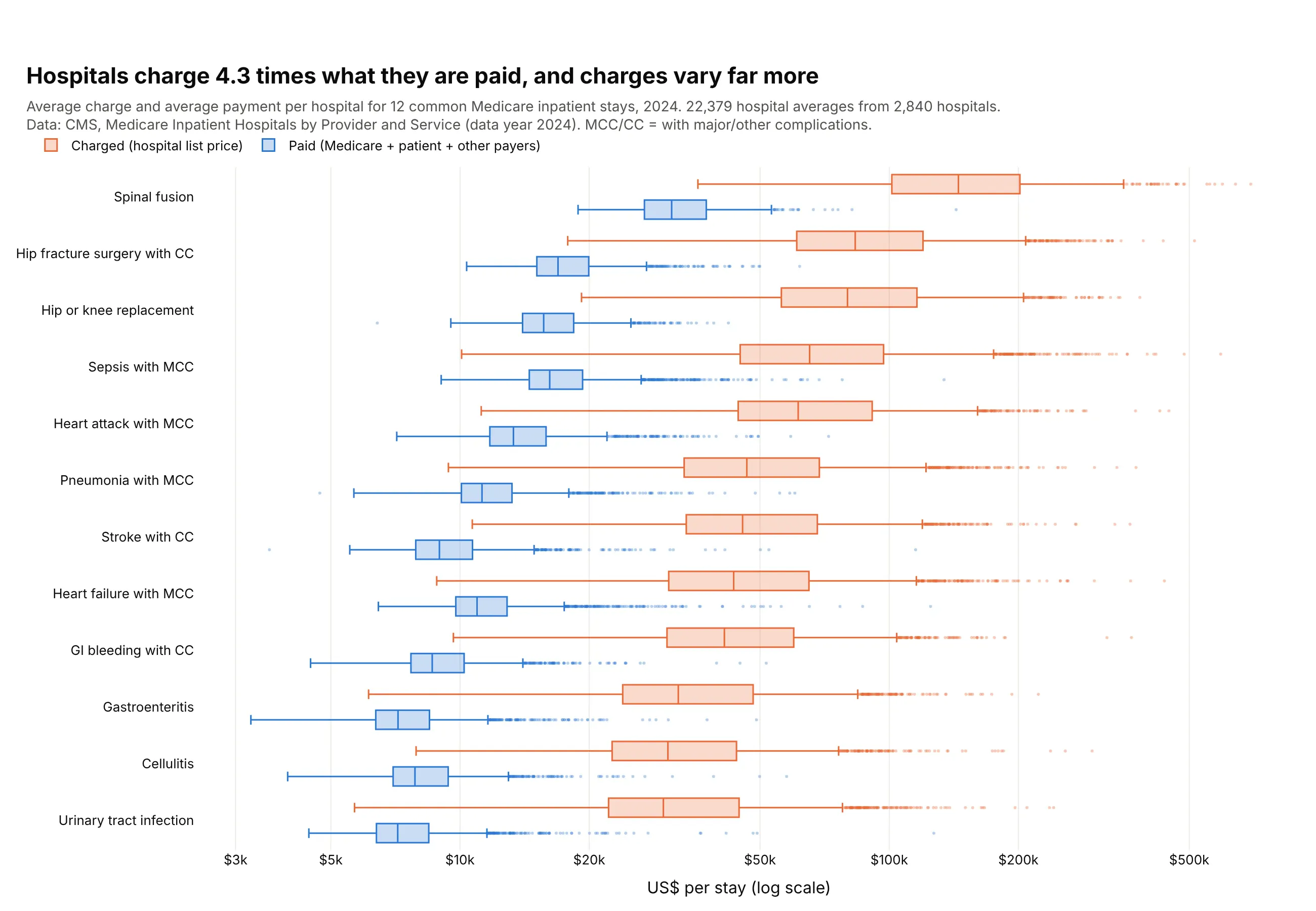
Prices across hospitals. Across 22,379 hospital averages for 12 common stays, hospitals charged a median 4.3 times what Medicare and other payers actually paid them. Data: CMS, Medicare Inpatient Hospitals by Provider and Service, 2024.

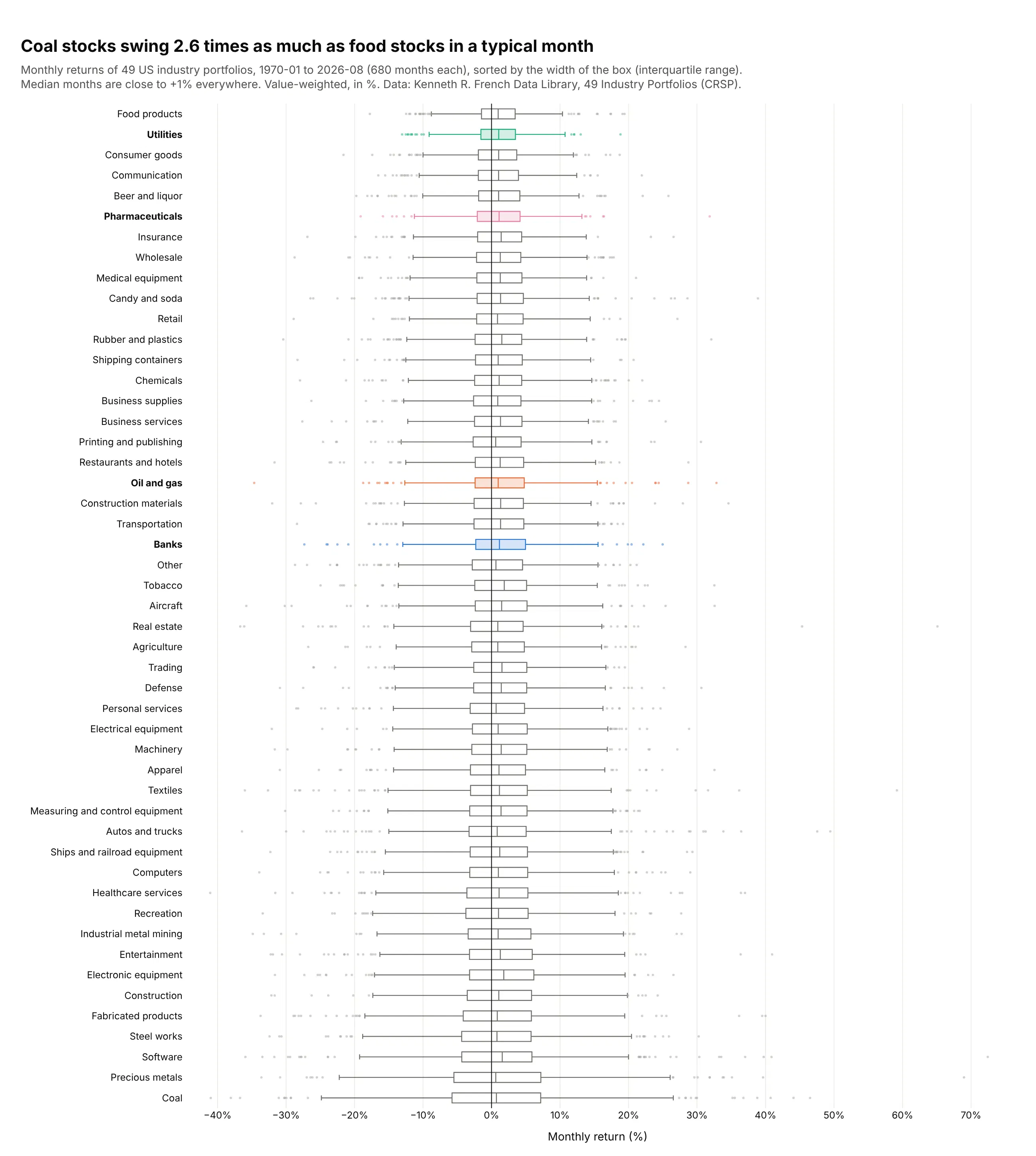
Risk across industries. Over 680 months the median month is between +0.6% and +1.9% for all 49 industries, but the middle half of coal's months spans 12.9 percentage points, 2.6 times food's 4.9. Data: Kenneth R. French Data Library, 49 Industry Portfolios, value-weighted, January 1970 to August 2026.

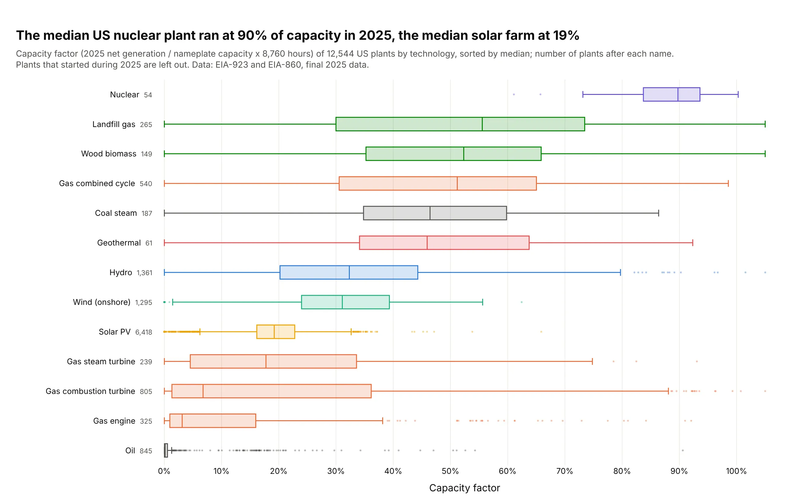
Performance across assets. The median US nuclear plant ran at 90% of its capacity in 2025 and the median solar farm at 19%, while gas plants span everything from 51% (combined cycle) to 7% (combustion turbines). Data: EIA-923 and EIA-860, final 2025 data.

To see what each part of a box means, here is one box taken apart, using all 4,073 hospitals from the ER example at once:

A short history

Mary Eleanor Spear drew a "range bar" with a box for the middle half and a median line in Charting Statistical Data (1952). John Tukey turned it into the box-and-whisker plot in Exploratory Data Analysis (1977), with whiskers that stop at 1.5 times the interquartile range and outliers drawn one by one, and a year later Robert McGill, Tukey and Wayne Larsen added notches in "Variations of Box Plots" (The American Statistician, 1978). Here are the three forms redrawn with Plotly on Albert Michelson's 1879 speed of light measurements, five experiments of 20 runs each:

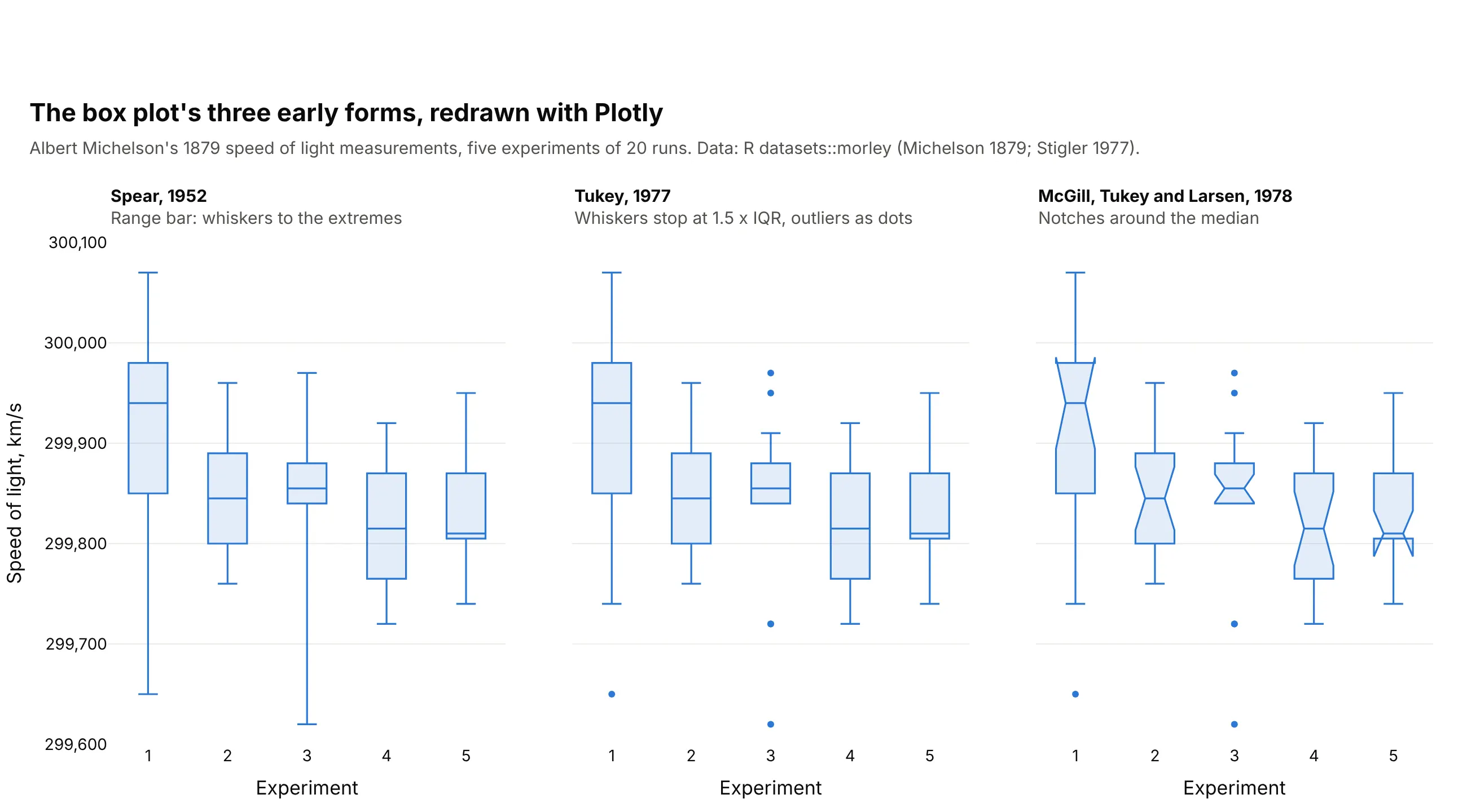
Michelson's first experiment came out at a median 299,940 km/s, 100 km/s above the other four, and its notch doesn't overlap theirs. In 1989, Michael Frigge, David Hoaglin and Boris Iglewicz found that statistical packages drew different boxes for the same data, because they computed quartiles differently, which is still true today (see the FAQ).

Alternatives to a box plot

Here's the same ER data for three states drawn six ways. Some are better for the question, some worse, some just different:

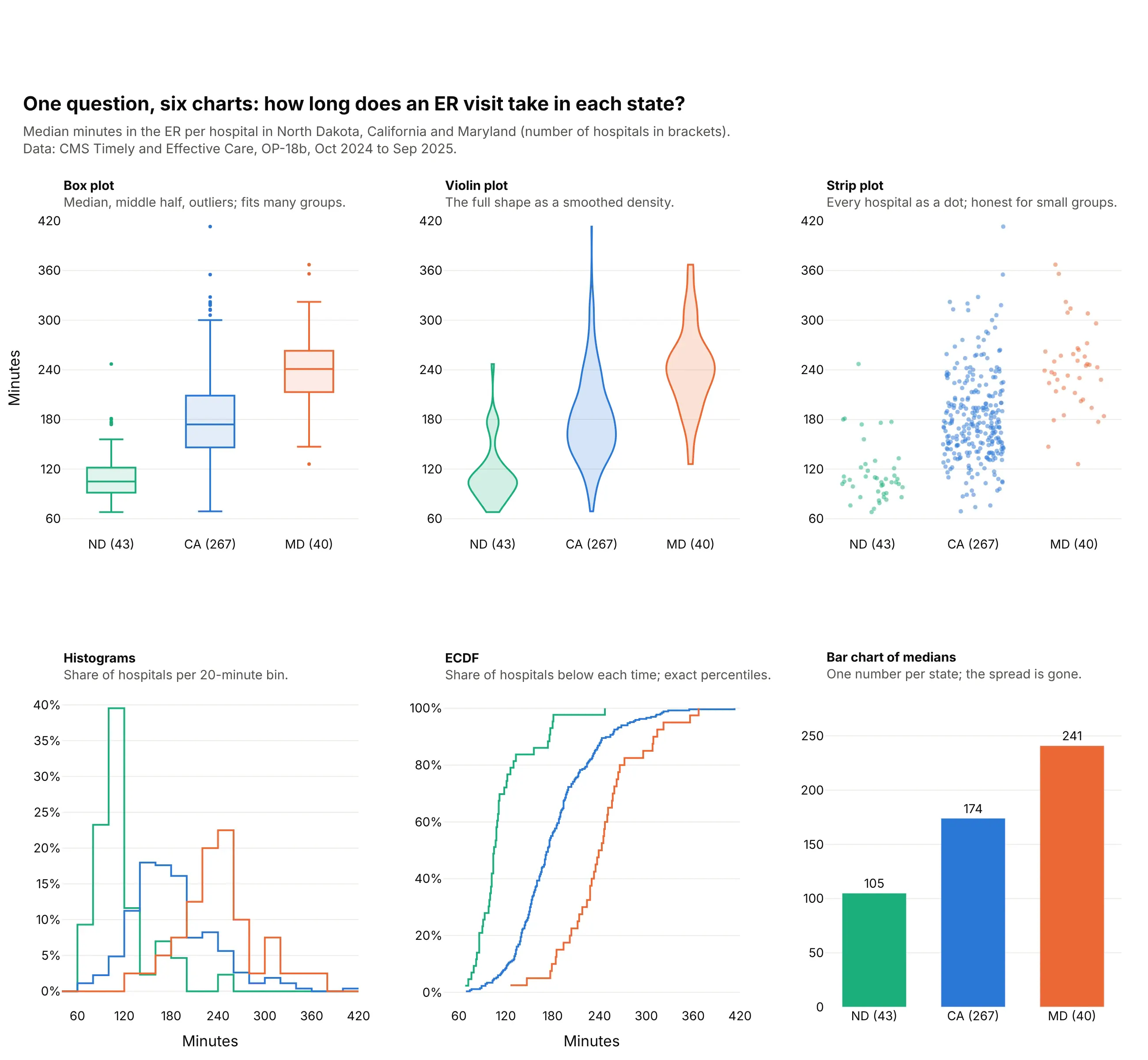
• Violin plot (different, better for shape). It draws the whole distribution as a smoothed density, so it shows two peaks or a gap that a box hides, at the cost of more ink per group. See our violin plot guide.
• Strip plot (better for small groups). Every value is a dot, which is the most honest view when a group has fewer than about 50 values and unreadable when it has thousands. Plotly can draw the dots on top of the box with boxpoints="all".
• Histogram (better for one distribution). It shows the shape of a single group in detail, but three overlaid histograms are already hard to read and 50 are impossible. See our histogram guide.
• ECDF (different). Each line shows the share of hospitals below each time, so you can read any percentile exactly, but most readers need it explained.
• Bar chart of medians (worse). One number per group is easy to read, but it hides the spread, which is often the story. Maryland's median (241 minutes) is 2.3 times North Dakota's (105), and the bars can't show that North Dakota's slowest hospital (247 minutes) takes longer than Maryland's median.

Here's where the histogram wins. A single box of 1,909 US gas plants looks like an ordinary skewed group, while the histogram shows two kinds of plants, 678 peakers that ran under 5% of the time and a broad hump of plants between 40% and 70%:

How to make a box plot

With AI

ChatGPT, Claude Code, GitHub Copilot, Cursor and other AI tools are excellent at writing Plotly code. Name Plotly in the prompt, describe the groups and the value, and list the checks you want:

The last check catches the most common bug in box plot reporting, which is quoting quartiles from pandas that don't match the chart.

With Plotly Studio

Plotly Studio is a desktop app where you point an AI at a dataset and it builds charts and a Dash app around your questions. Ask for a box plot the same way:

Show a box plot of emergency department time by state, one box per state sorted by median, with the number of hospitals under each state. Add a dropdown to switch between states and hospital types, and a table of the slowest hospitals in the selected state.

Make a box plot in Python or JavaScript

This is the code AI tools write under the hood. In Python, Plotly Express draws one box per group from a tidy table with one row per value:

When the data is too big to send to the browser, compute the statistics first (in pandas, SQL or Spark) and pass them to go.Box instead of the raw values:

In JavaScript, plotly.js takes one trace per box with its raw values. These are the first two of Michelson's 1879 experiments:

Share it

Every Plotly chart has a Share chart button (the cloud icon in its toolbar) that uploads it to Plotly Cloud and gives you a link. Only you can see it until you change its visibility.

For a live app, put the chart in a Dash app and publish it with the Plotly Cloud CLI. Coding agents can run these commands for you:

If your data has to stay in your own cloud or data center, publish to Dash Enterprise instead.

Dos and don'ts

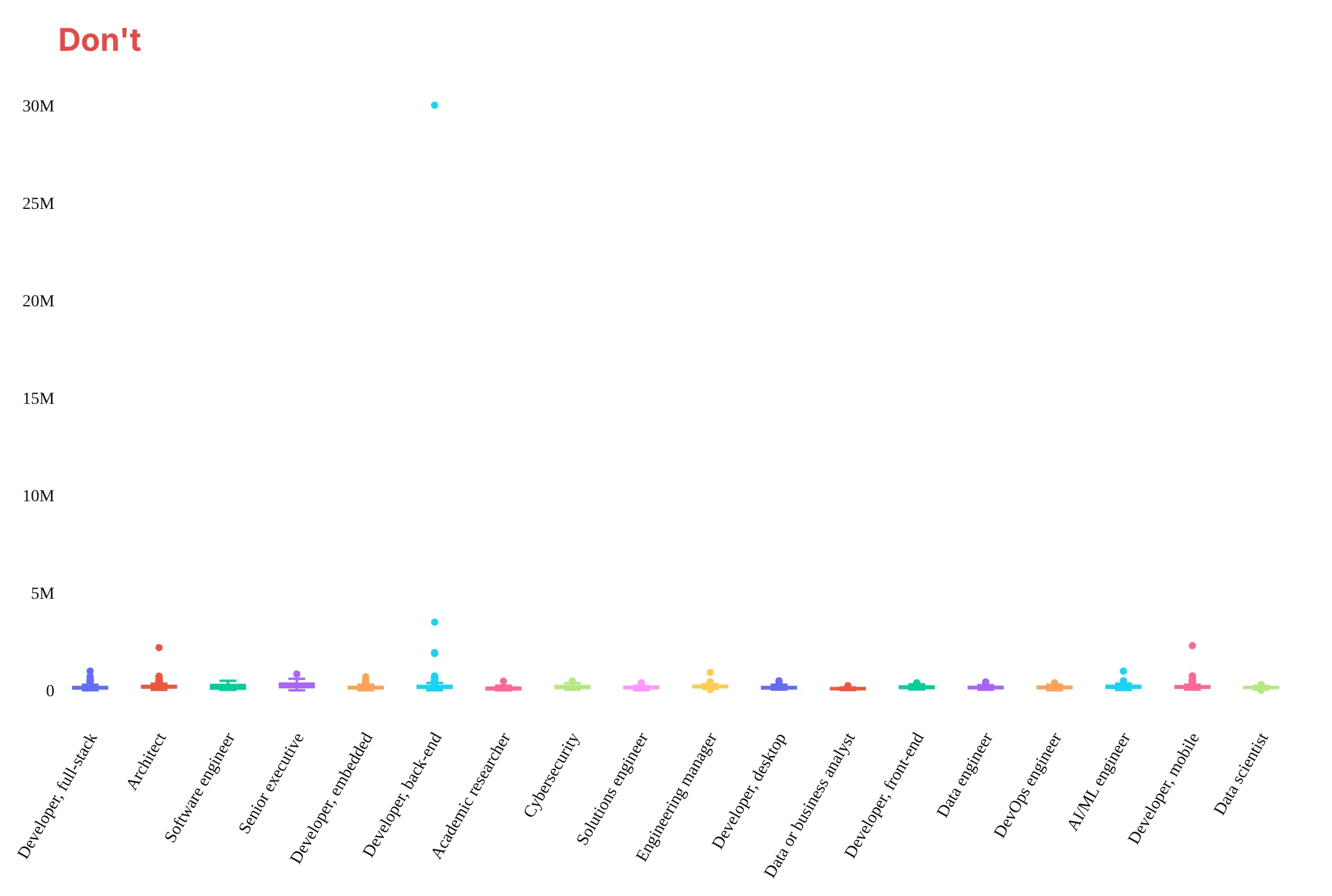
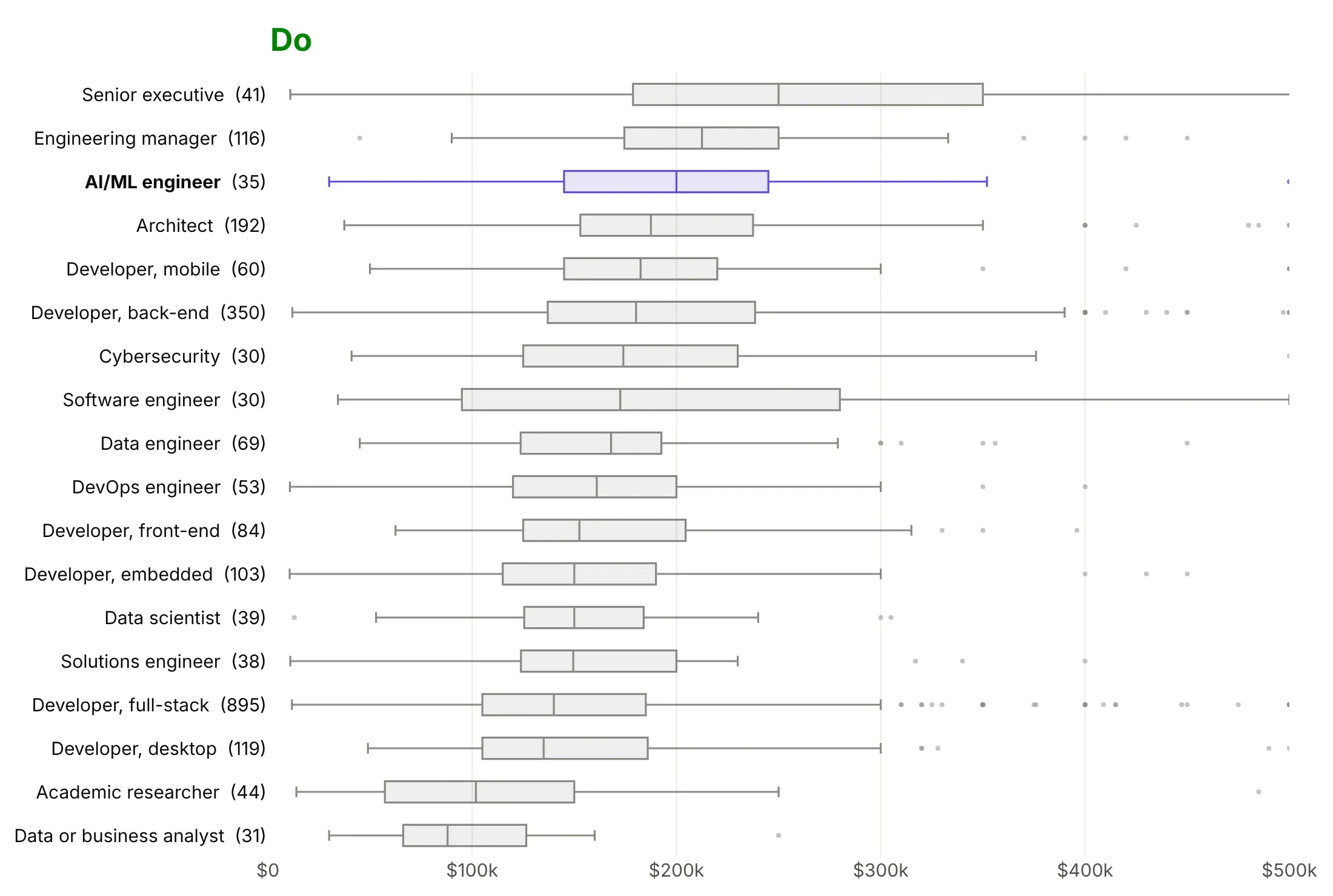
Plotly's defaults are made for exploring. For a published chart, most of the work is deciding what to leave out. Here are the yearly salaries of 2,329 US developers in 18 roles from the Stack Overflow Developer Survey 2026, drawn both ways.

Don't plot the groups in file order with rotated labels and a color per box, or let one $30 million answer set the axis, which squashes every box flat:

Do draw horizontal boxes sorted by median, gray with the one role the story is about in color, put the count after each role and cap the axis at $500k. Say on the page that 36 answers are above the cap:

Show as much of the data as the question needs

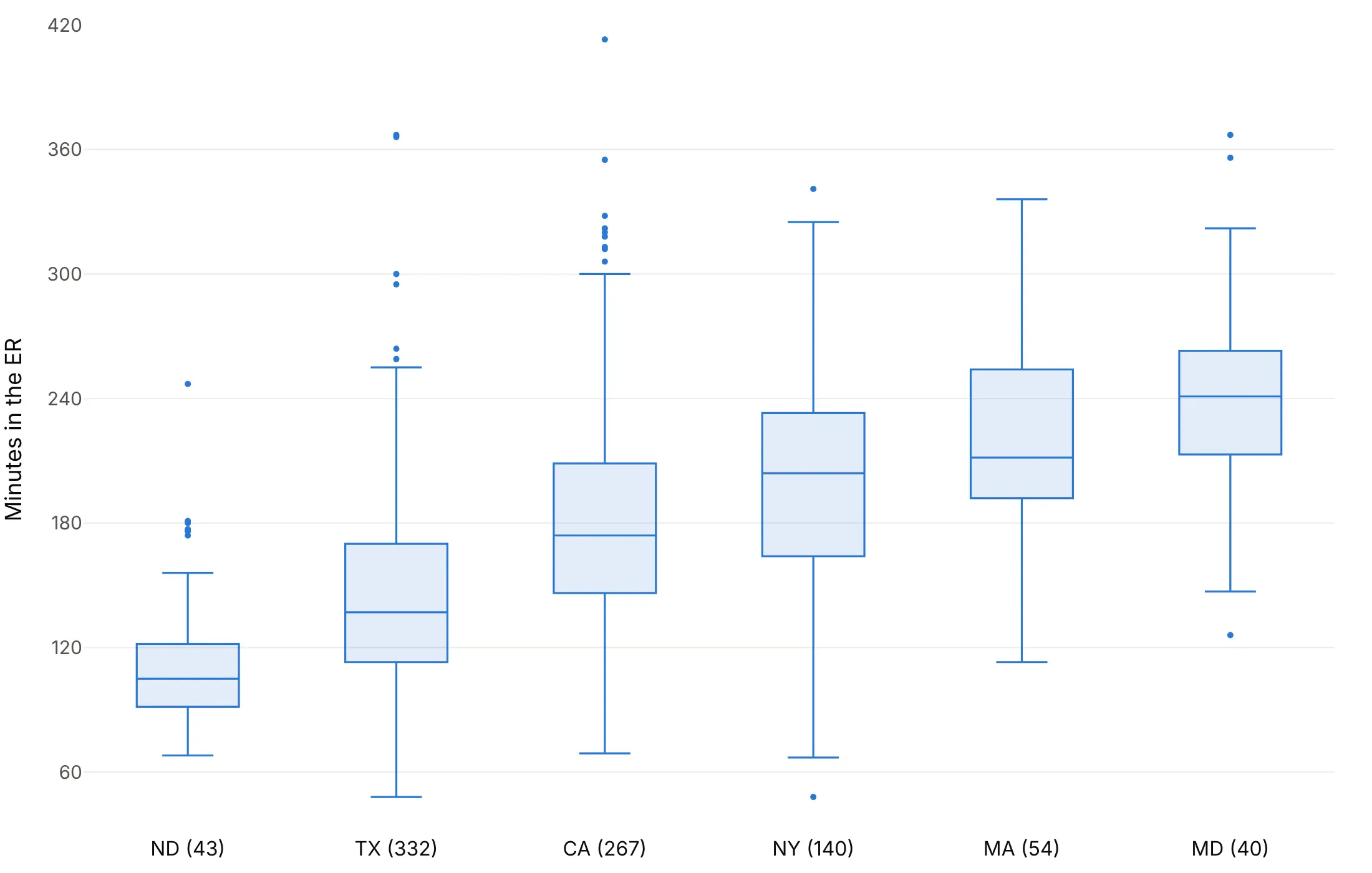
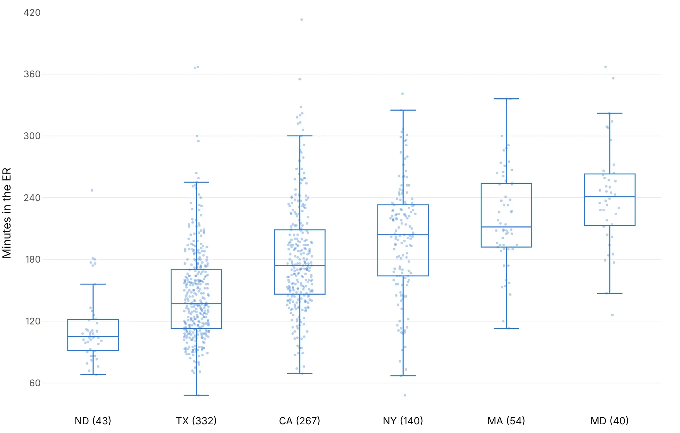
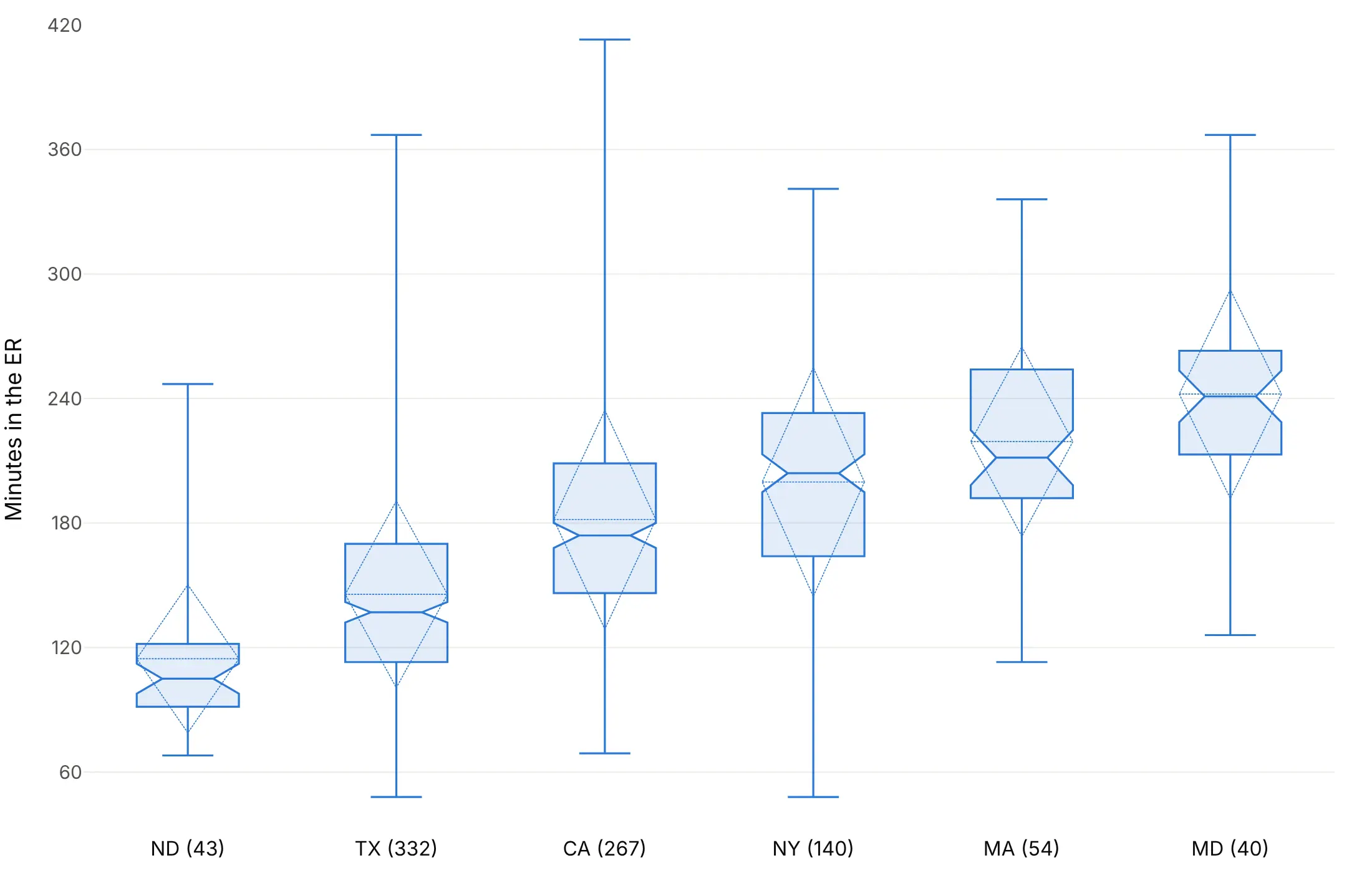
The other big choice is how many of the values to draw. Here are four options on the ER times of hospitals in six states, with the number of hospitals after each state.

Outlier dots only. Plotly's default (boxpoints="outliers"), and the right one for large groups.

Every value. boxpoints="all" with jitter puts each hospital on its box, which shows how few hospitals stand behind the North Dakota and Maryland boxes.

Notches, mean and standard deviation. notched=True answers whether two medians really differ, and boxmean="sd" adds the mean and one standard deviation. With boxpoints=False the whiskers move to the minimum and maximum.

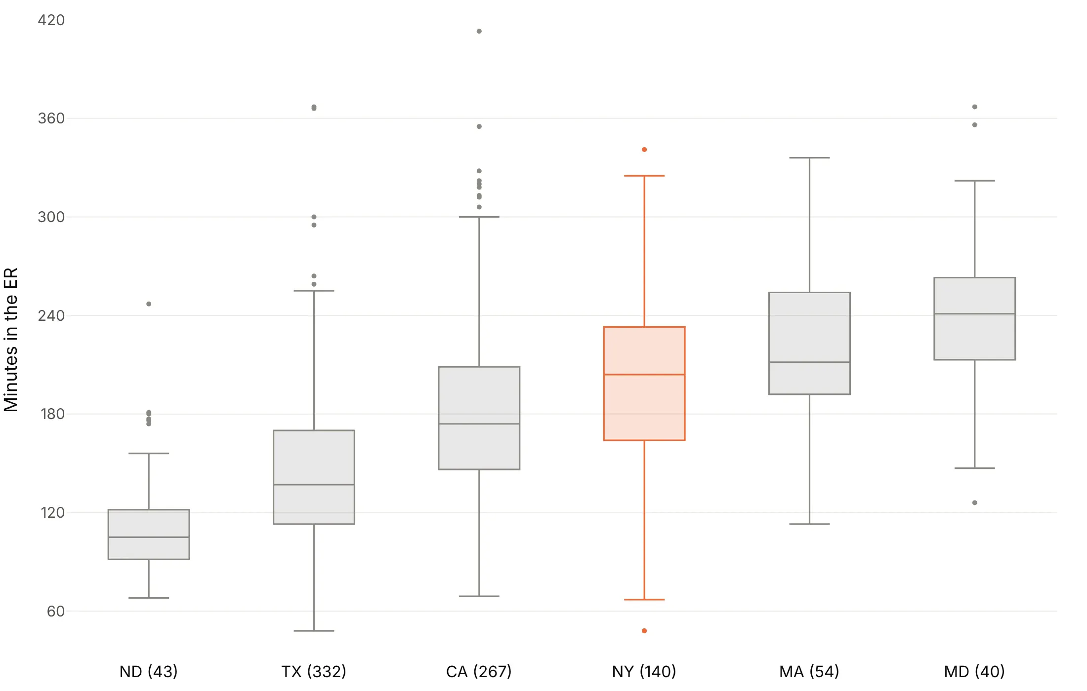
One story. Gray boxes with one state in color, here New York, when the title is about one group.

Checklist

Do

• Write a title that states the takeaway.
• Sort the groups by median, or by IQR when spread is the story, unless they have a natural order like months.
• Go horizontal when labels are long, with orientation="h" or the values on x.
• Print the count next to each group label, because a box of 21 values and a box of 1,438 look the same.
• Show every point for small groups with boxpoints="all", jitter and pointpos.
• Cap the axis when a few extreme values squash the boxes, and say how many points are off the chart.

Don't

• Plot in file order with rotated labels.
• Color each box differently unless the color means something.
• Trust a single box for data that might have two groups in it.
• Hide outliers silently, since boxpoints=False also moves the whiskers to the minimum and maximum.
• Put two $ signs in one title or label, which makes Plotly render it as LaTeX; write $ for one of them.

Options to customize

These are the go.Box (and px.box) options that matter most. The full list is in the Plotly box plot documentation.

1. x, y: the values and the group of each value; put the values on x with orientation="h" for horizontal boxes.
2. orientation: "v" or "h"; horizontal suits long group labels.
3. boxpoints: "outliers" (default), "suspectedoutliers", "all" or False; False also moves the whiskers to the minimum and maximum.
4. jitter, pointpos: how far points spread, and where they sit relative to the box (0 on it, -1.6 beside it).
5. notched, notchwidth, notchspan: notches at median ± 1.57 x IQR / √n, for comparing medians.
6. boxmean: True adds the mean as a dashed line, "sd" adds the standard deviation too.
7. quartilemethod: "linear" (default), "inclusive" or "exclusive", to match quartiles from another tool.
8. q1, median, q3, lowerfence, upperfence, mean, sd: precomputed statistics instead of raw values, for millions of rows.
9. sizemode, sdmultiple: draw the box as the mean ± k standard deviations, for audiences used to error bars.
10. marker.outliercolor, marker.line.outliercolor: the colors of mild outliers with "suspectedoutliers".
11. width, whiskerwidth: box width, and the whisker cap width as a share of it; setting width turns off automatic grouping.
12. offsetgroup, alignmentgroup: which boxes share a slot when you group boxes across traces.
13. boxmode, boxgap, boxgroupgap (layout): grouped or overlaid boxes and the gaps between them, for two categorical variables.
14. hovertemplate, customdata: hover content, for naming outliers (a hospital, a date, a driver).

More box plot examples

Ten more box plots built from real public data, each with its source, the technique that makes it work and a prompt to rebuild it.

1. Liver blood tests across the stages of hepatitis C

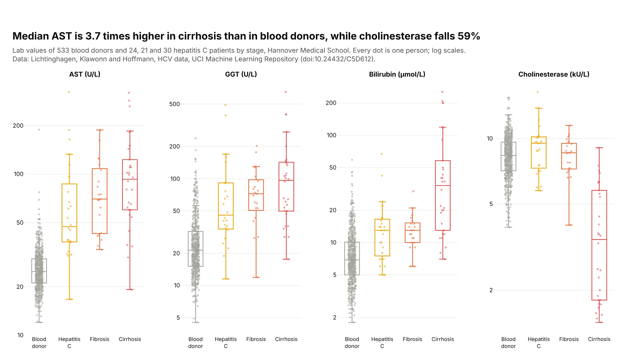
Median AST rises from 24.8 U/L in blood donors to 92.9 in cirrhosis, 3.7 times higher, while cholinesterase, which a working liver makes, falls 59%. With 21 to 30 patients per stage, every patient is drawn. Data: Lichtinghagen, Klawonn and Hoffmann, HCV data, UCI Machine Learning Repository (doi:10.24432/C5D612).

Tip: boxpoints="all" with pointpos=0 puts each patient on the box when groups are small.

2. Where the GLP-1 receptor is expressed

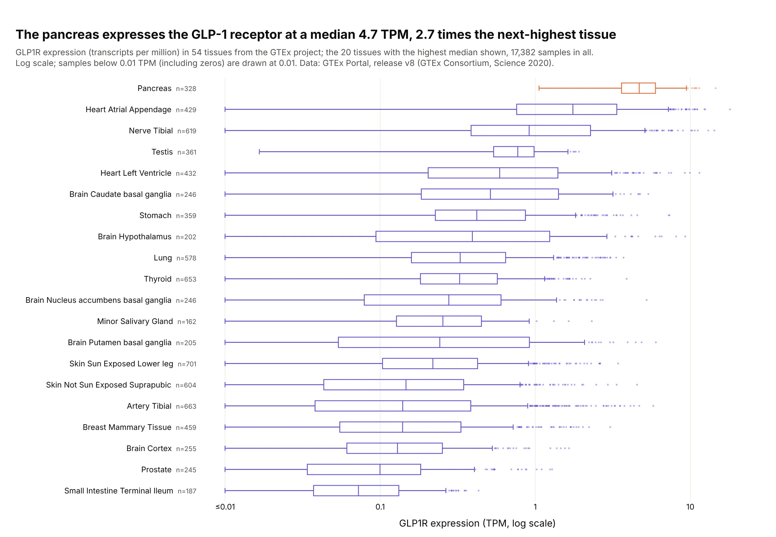
GLP1R, the receptor that semaglutide and tirzepatide act on, has a median 4.7 transcripts per million in the pancreas, 2.7 times the next tissue, and every pancreas sample is above 1 TPM. The stomach and the hypothalamus, both involved in appetite, follow at 0.42 and 0.39. Data: GTEx Portal, release v8, 17,382 samples (GTEx Consortium, Science 2020).

Tip: a log axis for skewed expression data, with zeros floored at 0.01 and the floor stated in the subtitle.

3. Bank efficiency by size, with notches

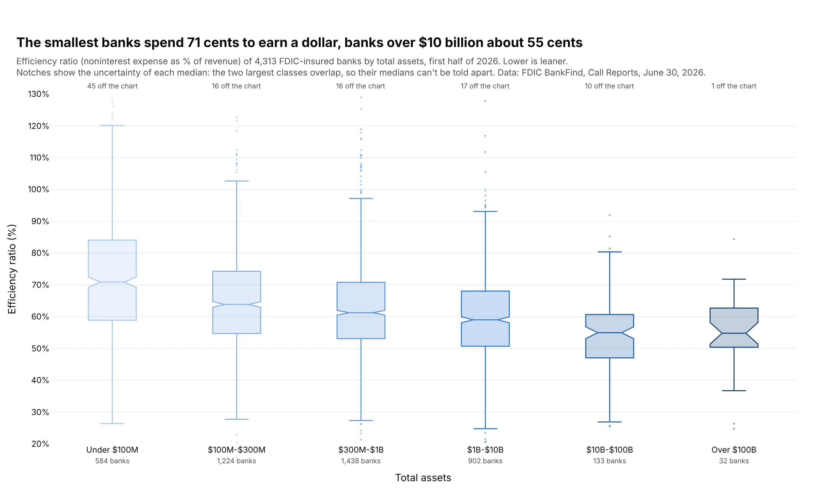
Banks under $100 million in assets spend a median 71 cents to earn a dollar of revenue, and banks over $10 billion spend about 55. The notches of the two largest classes overlap, so their medians can't be told apart. Data: FDIC BankFind Suite, Call Reports for June 30, 2026.

Tip: notched=True, with the axis capped at 20-130% and the banks outside counted above each box.

4. Demand at US Treasury auctions

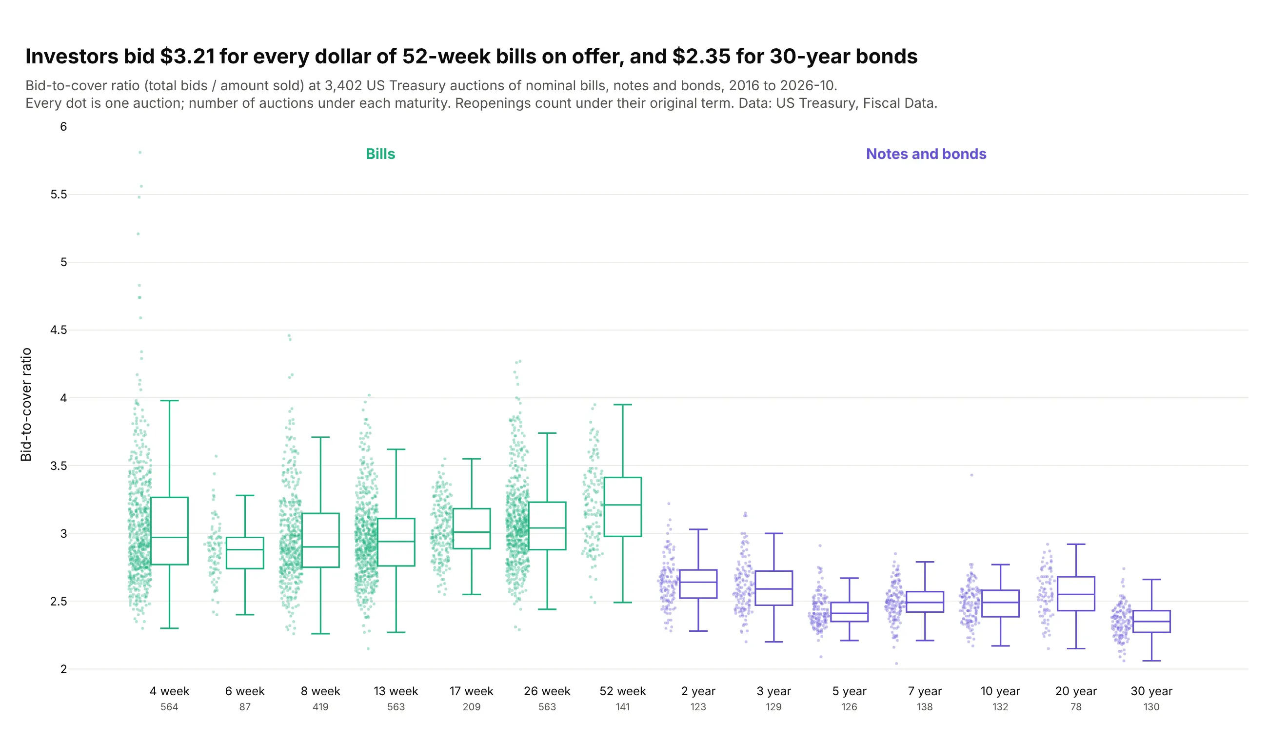
Since 2016, investors bid a median $3.21 for every dollar of 52-week bills on offer and $2.35 for 30-year bonds. Bills draw about 3 bids per dollar at every maturity, and demand thins as notes and bonds get longer. Data: US Treasury, Fiscal Data, Treasury Securities Auctions Data, January 2016 to October 2026.

Tip: pointpos=-1.6 draws the dots beside each box, so the number of auctions shows without hiding the box.

5. New York City's power price by hour

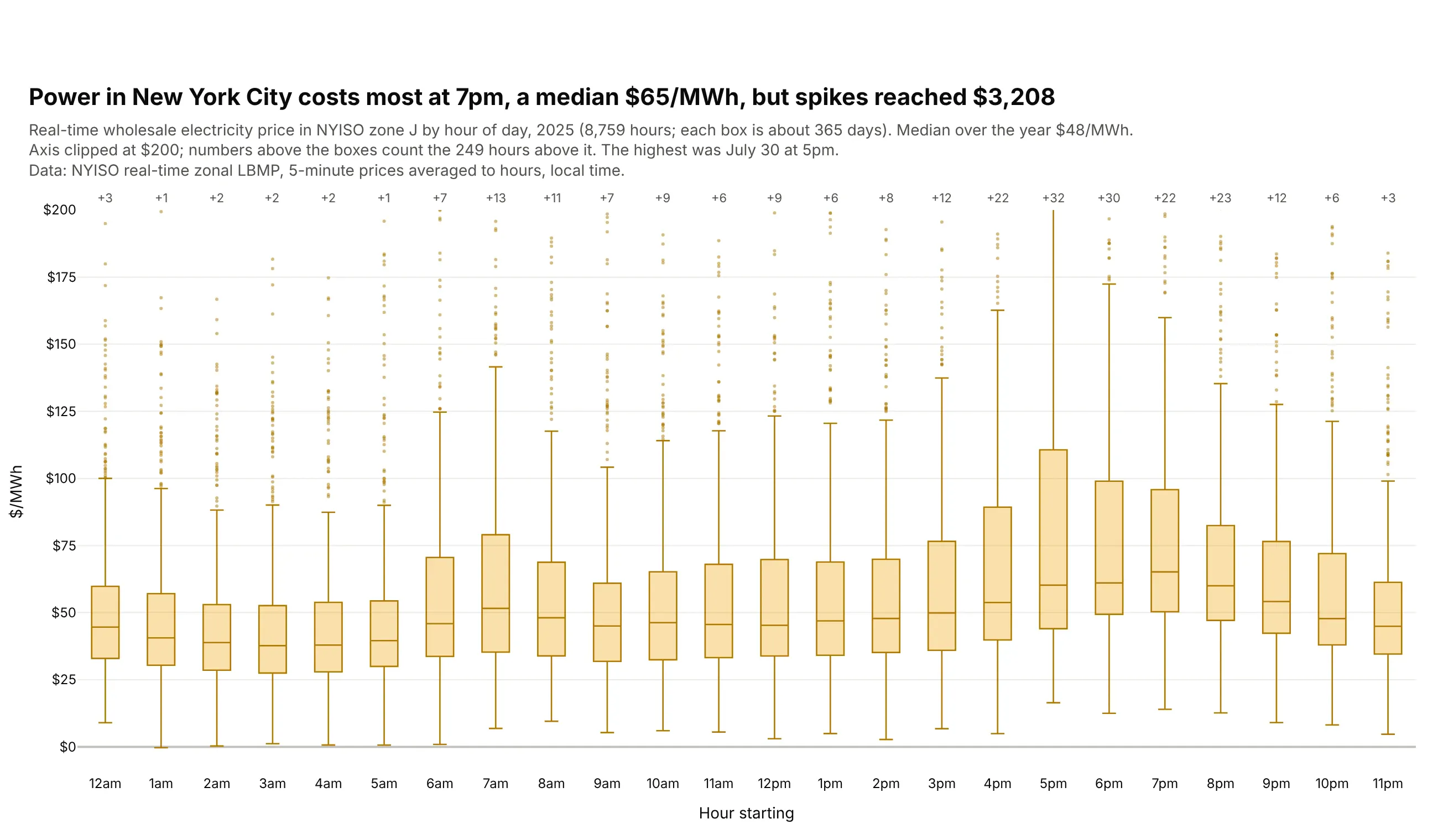
New York City's real-time power price peaks at a median $65/MWh at 7pm, against $38 at 3am. 249 hours cost more than $200, and on July 30 at 5pm the price reached $3,208. Data: NYISO real-time zonal LBMP, zone J, 2025.

Tip: clip the axis to where the boxes are and print the number of clipped values above each box.

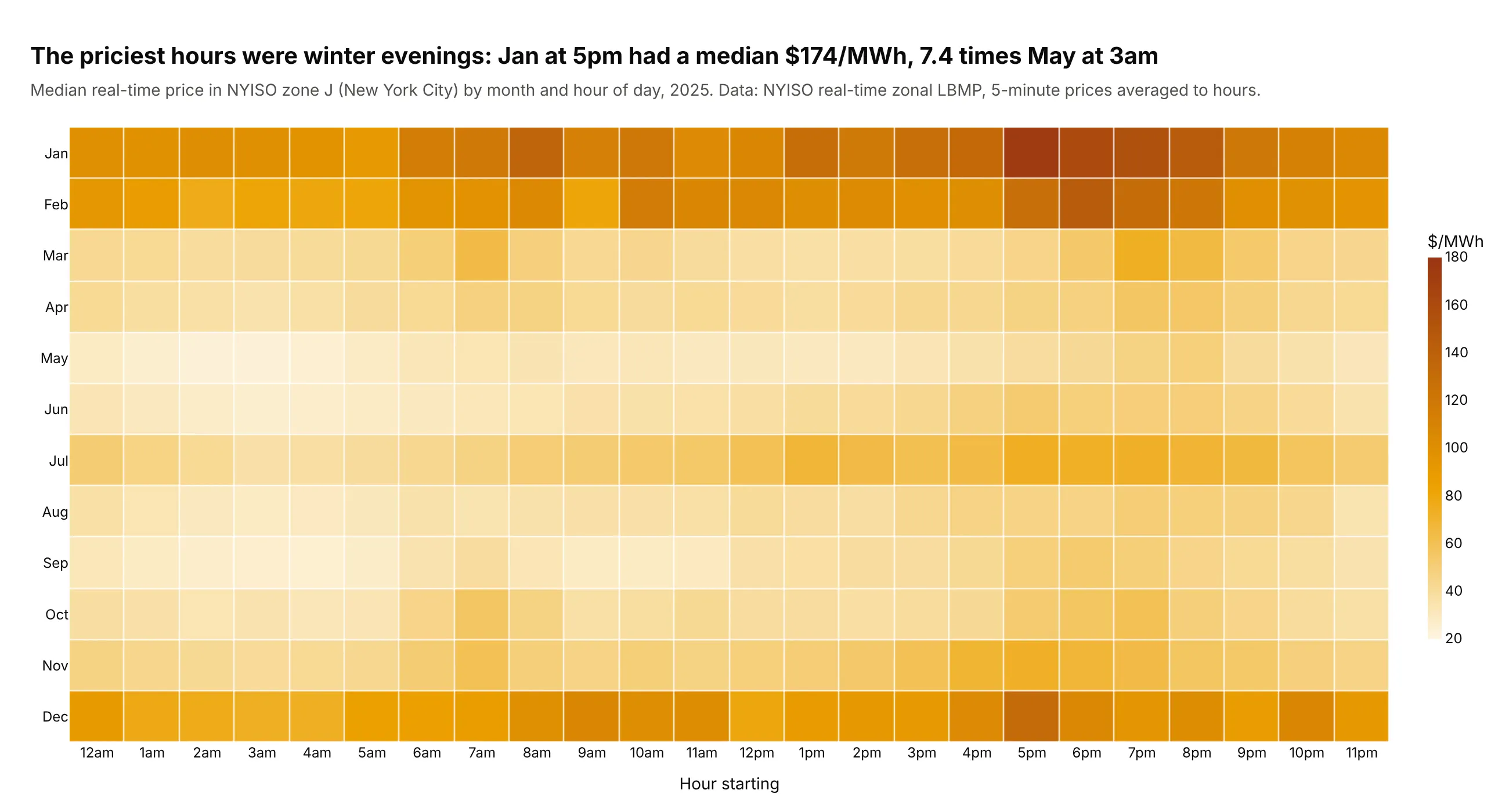
Another way to see it: a heatmap of the median price by month and hour shows when the expensive hours happen. January evenings were the priciest at a median $174, 7.4 times May nights.

6. Household power prices by region and ownership

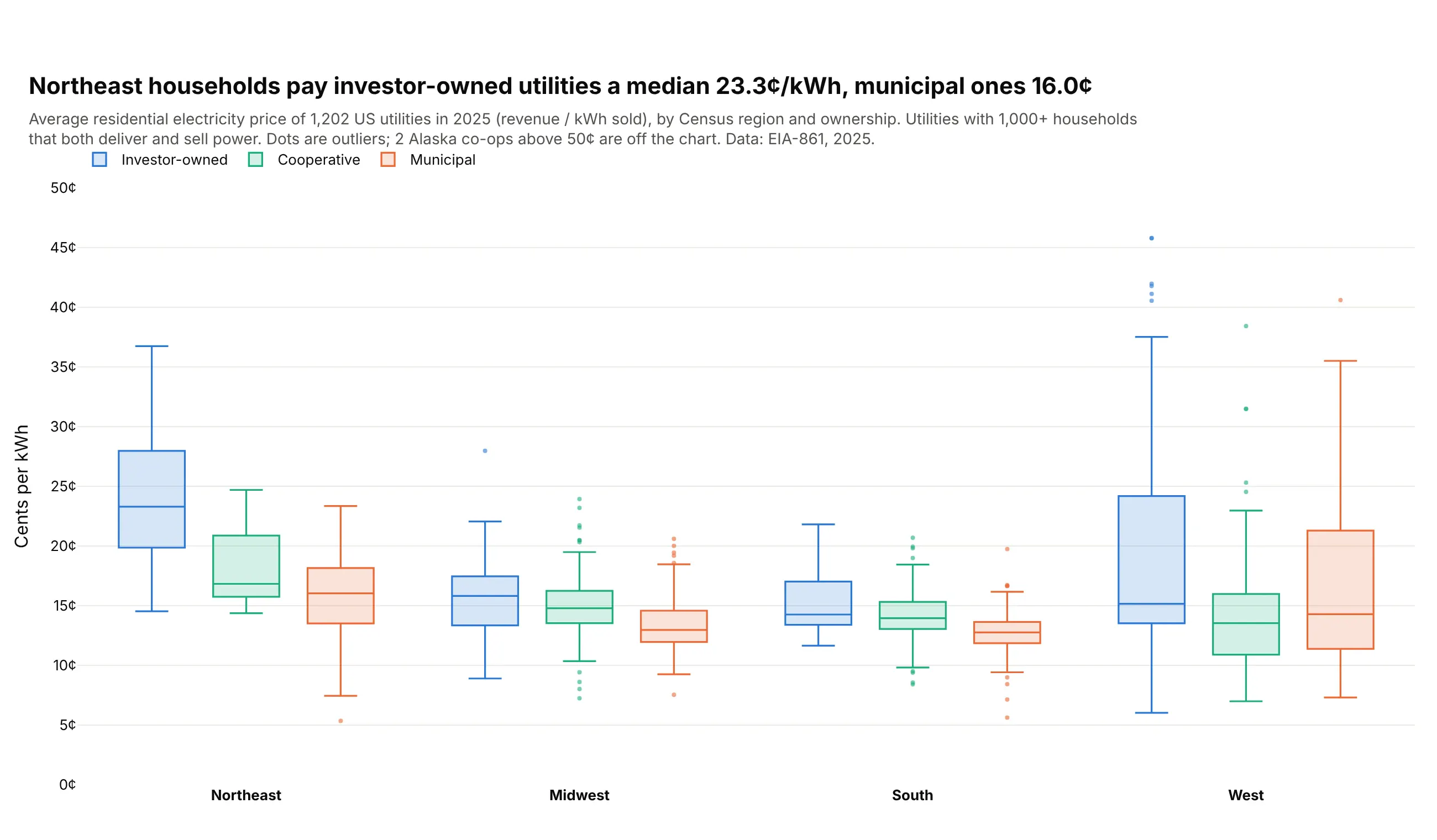
Northeast households pay investor-owned utilities a median 23.3 cents per kWh and municipal ones 16.0. In the Midwest and South the three kinds of utility sit within 3 cents of each other, and the West has the widest spread. Data: EIA-861, 2025.

Tip: boxmode="group" with the same ownership order and colors in every region.

7. New York's air in the year of the wildfire smoke

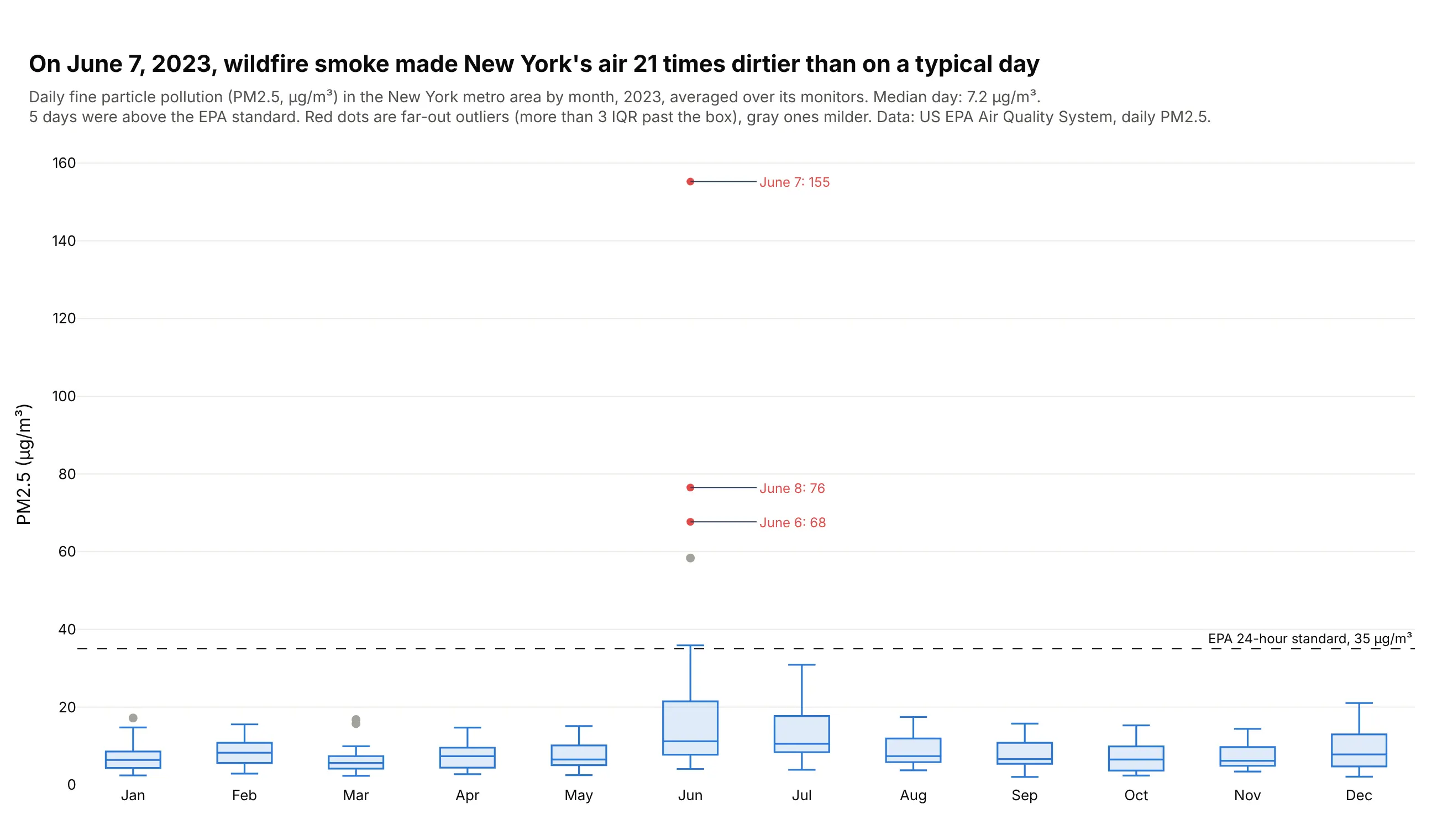
On a typical day in 2023, New York's air had 7.2 µg/m³ of fine particles. On June 7, smoke from Canadian wildfires pushed it to 155, 21 times as much, and five days broke the EPA's 24-hour standard. Data: US EPA Air Quality System, daily PM2.5, New York-Newark-Jersey City metro area, 2023.

Tip: boxpoints="suspectedoutliers" separates mild outliers from far-out ones, so the smoke days stand out in red.

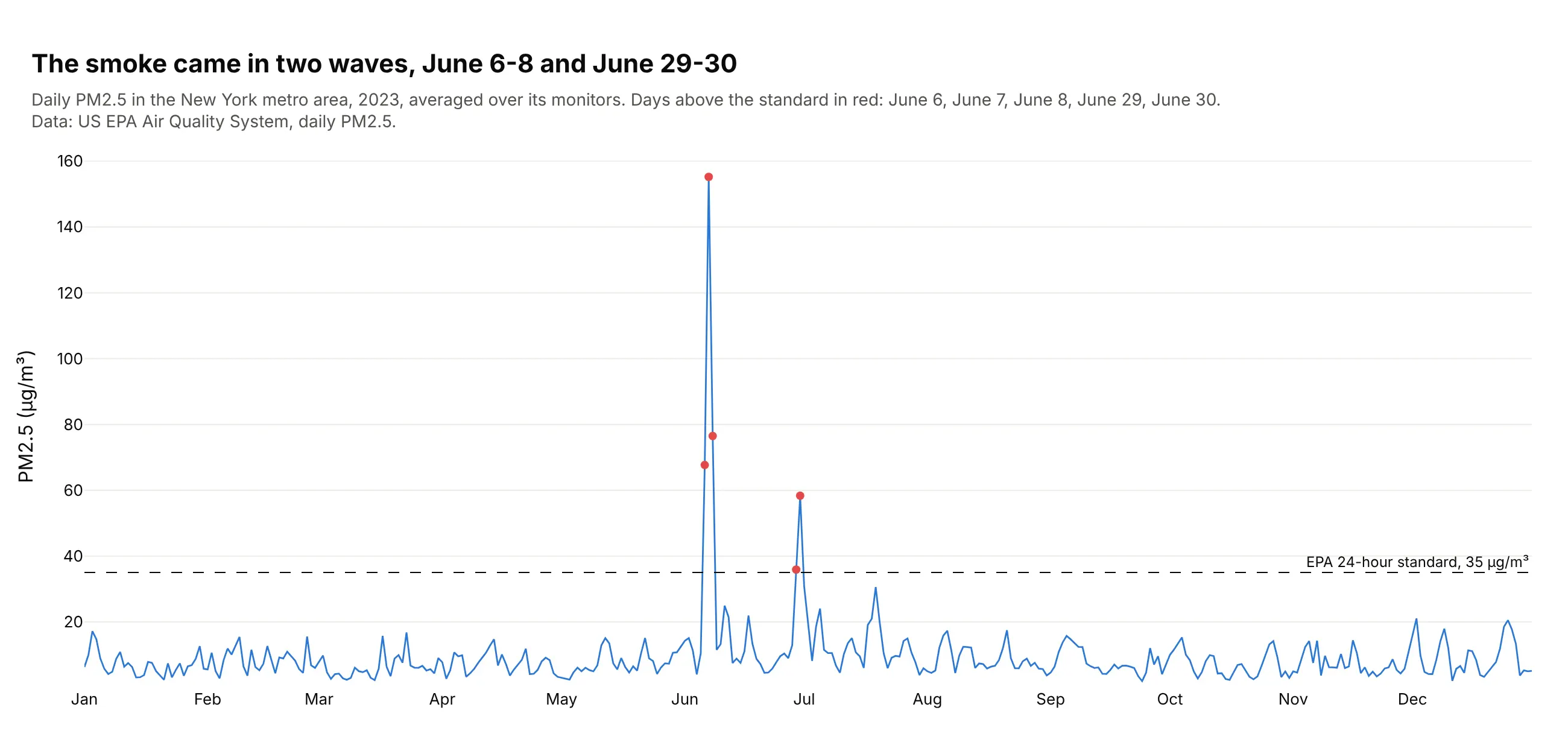
Another way to see it: the daily values as a line show that the smoke came in two waves, June 6-8 and June 29-30, which a monthly box can't separate.

8. US developer salaries by role

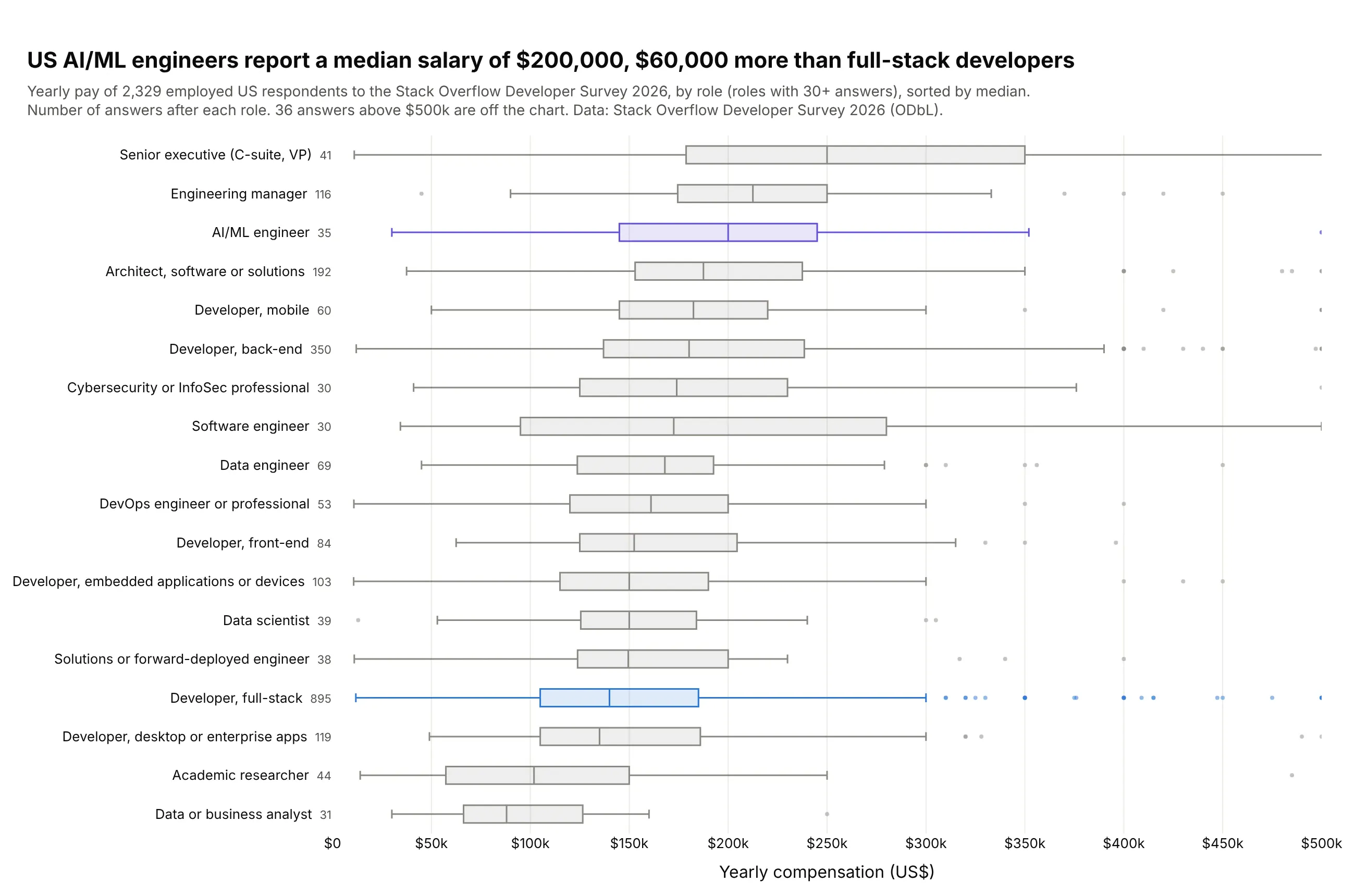
US AI/ML engineers report a median $200,000, $60,000 more than full-stack developers. Only 35 AI/ML engineers answered, against 895 full-stack developers, which is why the count sits next to each role. Data: Stack Overflow Developer Survey 2026 (ODbL).

Tip: cap the axis and state how many answers are beyond it (36 here), so one $30 million answer doesn't flatten every box.

9. 6.9 million flights from 14 rows of statistics

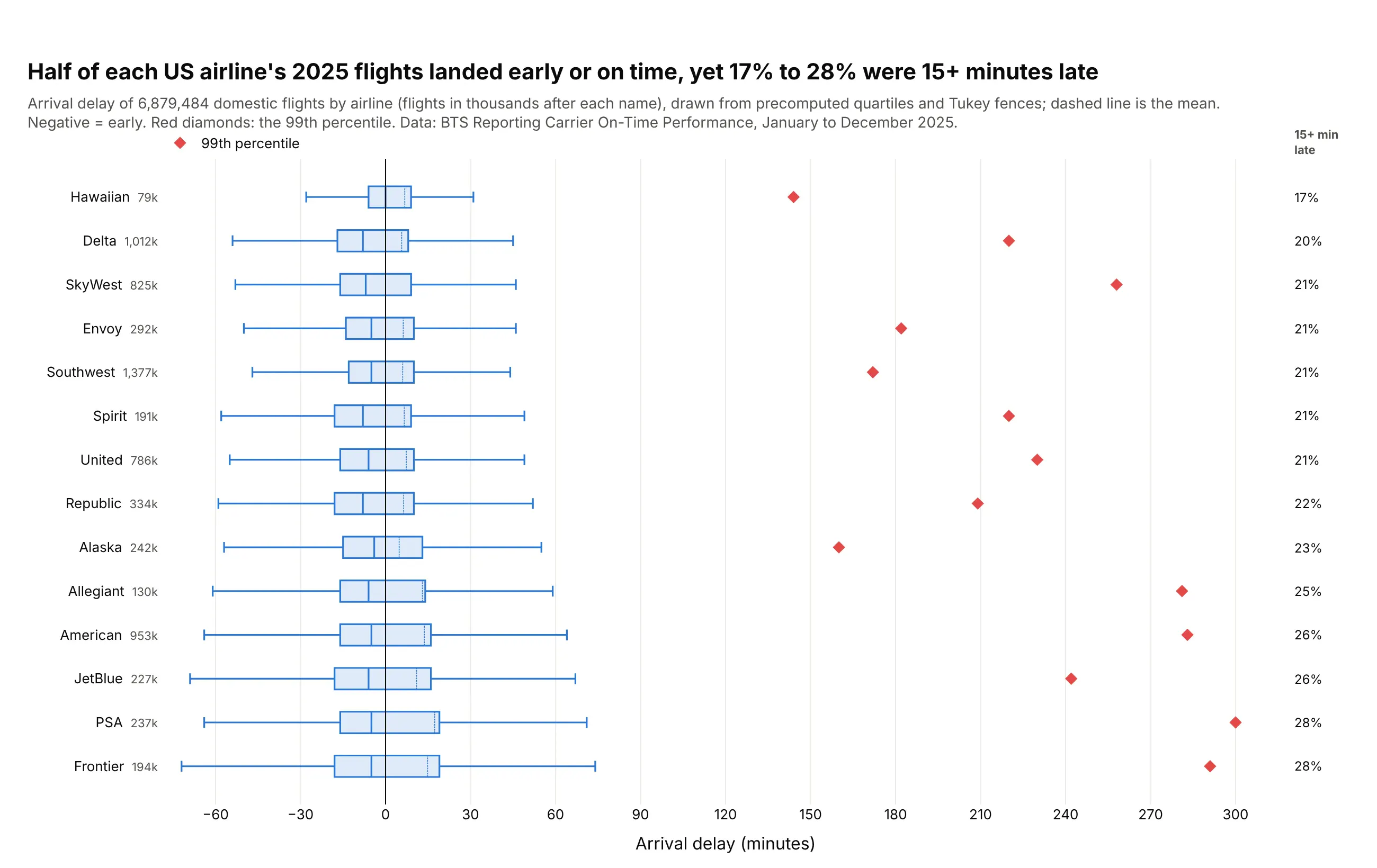
On every US airline in 2025, at least half the flights landed early or on time, yet 17% (Hawaiian) to 28% (Frontier) arrived 15 minutes or more late. The 99th percentile reaches 144 to 300 minutes, which pulls every airline's mean delay above zero. Data: BTS Reporting Carrier On-Time Performance, January to December 2025.

Tip: pass q1, median, q3, lowerfence, upperfence and mean to go.Box instead of the raw rows.

10. Every lap of the 2025 Abu Dhabi Grand Prix

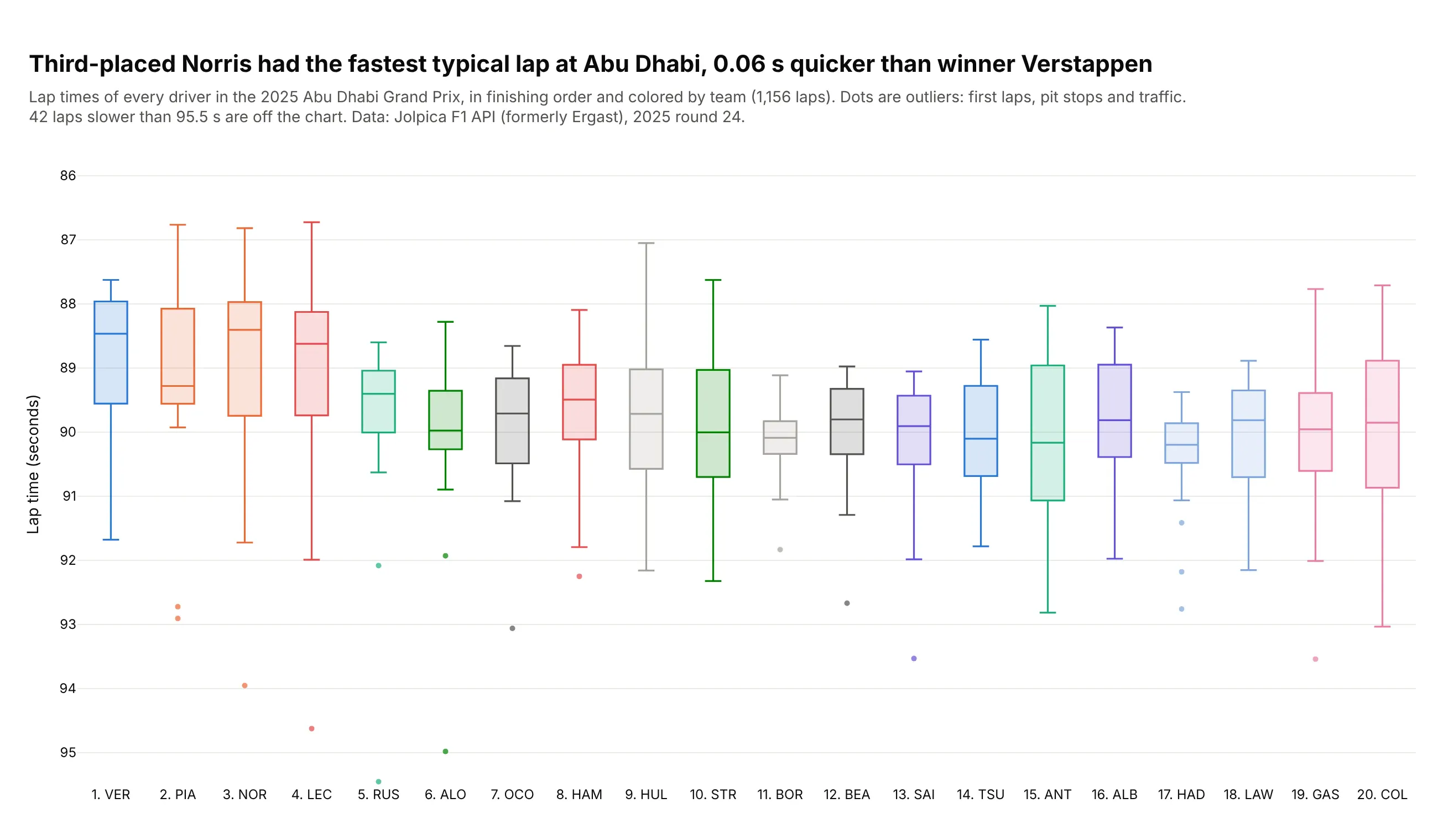
Lando Norris finished third but had the fastest median lap, 88.40 seconds, 0.06 s quicker than the winner Max Verstappen. The outliers are first laps, pit stops and traffic, so the box shows race pace better than an average would. Data: Jolpica F1 API (formerly Ergast), 2025 round 24.

Tip: reverse the y axis so faster is higher, and zoom it to 10 seconds so tenths show.