Heatmaps - A Complete Guide

TL;DR

• A heatmap draws a table of numbers as a grid of colored cells, with two categories (or two binned axes) as rows and columns and color for the value, so patterns across hundreds or millions of cells show at once.
• Heatmaps are also known as heat maps and shaded matrices, and are similar to calendar heatmaps, hexbin plots and contour plots.
• Use one for matrices (correlations, flows, drug x reaction counts), for a value across two time scales (hour x day, month x year) and for the density of point data. Use a line or bar chart when readers need exact values for a few series.
• The color scale and the order of rows and columns are the two decisions that matter: sequential, diverging with zmid, log or binned color, and rows sorted or clustered so similar ones sit together.
• Any coding agent can make one with Plotly in a minute. In Python it's px.imshow(df, text_auto=True).

What is a heatmap?

Heatmaps look like this:

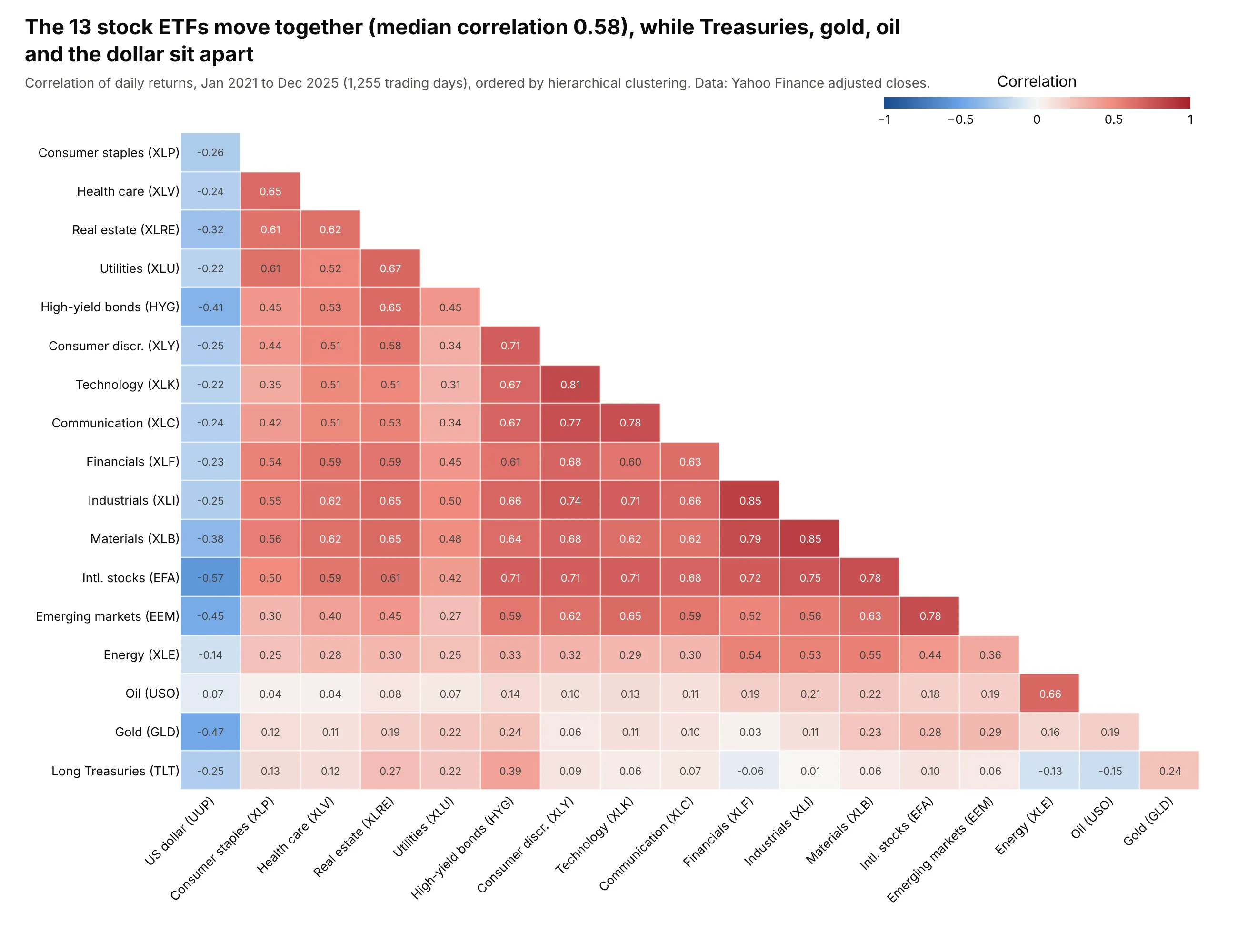
Data: Yahoo Finance adjusted daily closes, 2021-2025.

How do you read a heatmap? In the example above, notice these things:

• Each cell is one pair of ETFs, and its color shows the correlation of their daily returns, so the darker the red, the more closely the two moved together.
• The color scale is centered on zero, so white cells are pairs with almost no correlation, and the grid splits at a glance into pairs that rose and fell together (red) and pairs that moved in opposite directions (blue).
• The rows and columns are ordered by clustering, which puts similar assets next to each other, so the stock ETFs and high-yield bonds form one large red block in the middle of the chart, and oil sits next to energy stocks, the one stock ETF it moved with.
• Only the lower triangle is drawn because the matrix is symmetric, and each cell prints its value, so you can read off a pair like financials and industrials at 0.85.
• The US dollar column on the left is blue all the way down, while the pale rows for gold and long Treasuries at the bottom mean those assets barely moved with stocks, which is different from moving against them.

It's often used for charts like these:

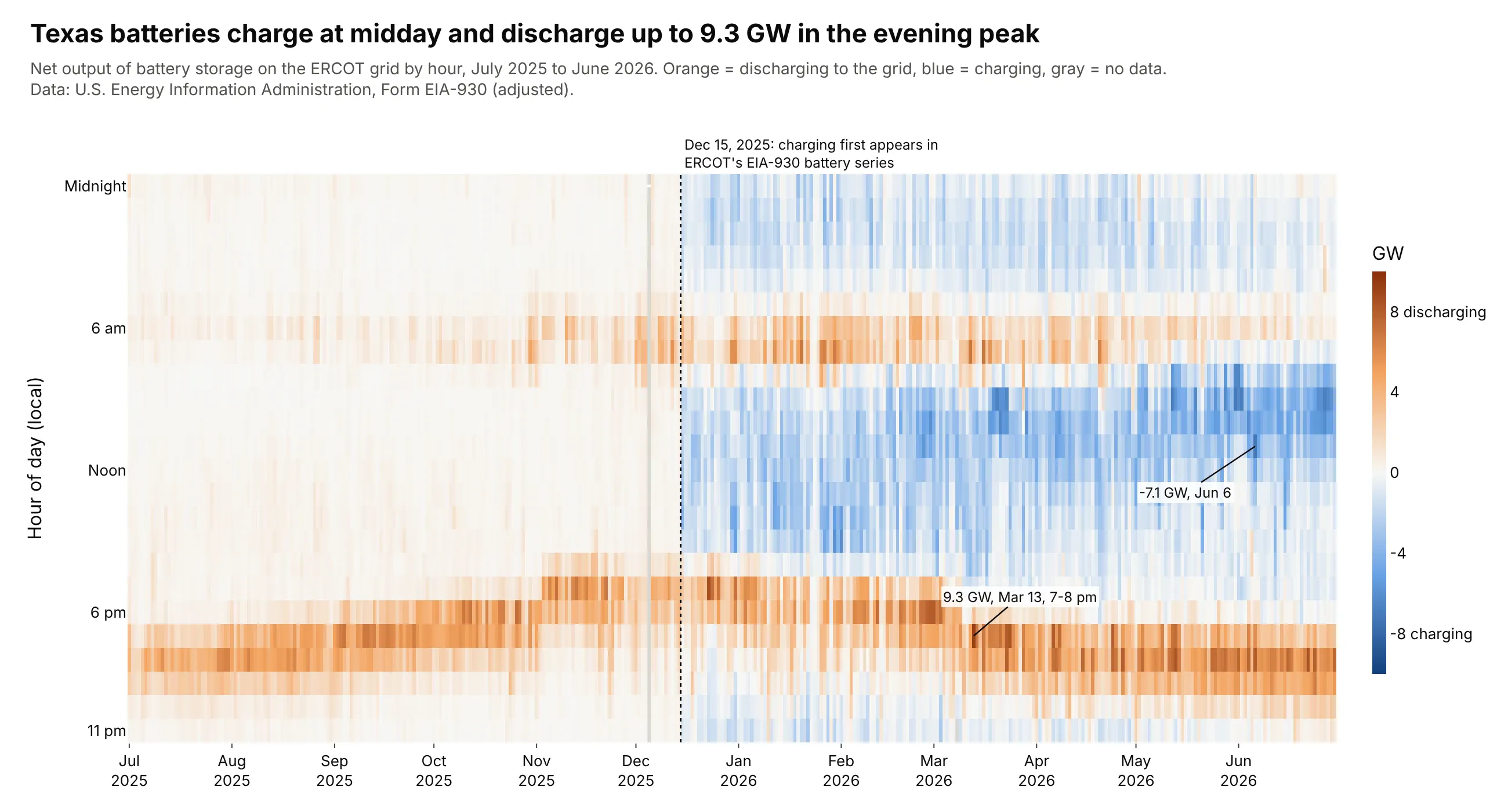
An hour x day grid. Folding 8,760 hours of Texas battery output into one grid shows the batteries discharging into the evening peak, up to 9.3 GW on March 13, 2026, and charging at midday from December 15, 2025, when ERCOT's EIA-930 series starts reporting negative values. Data: U.S. EIA, Form EIA-930, ERCOT battery storage net generation, July 2025 to June 2026.

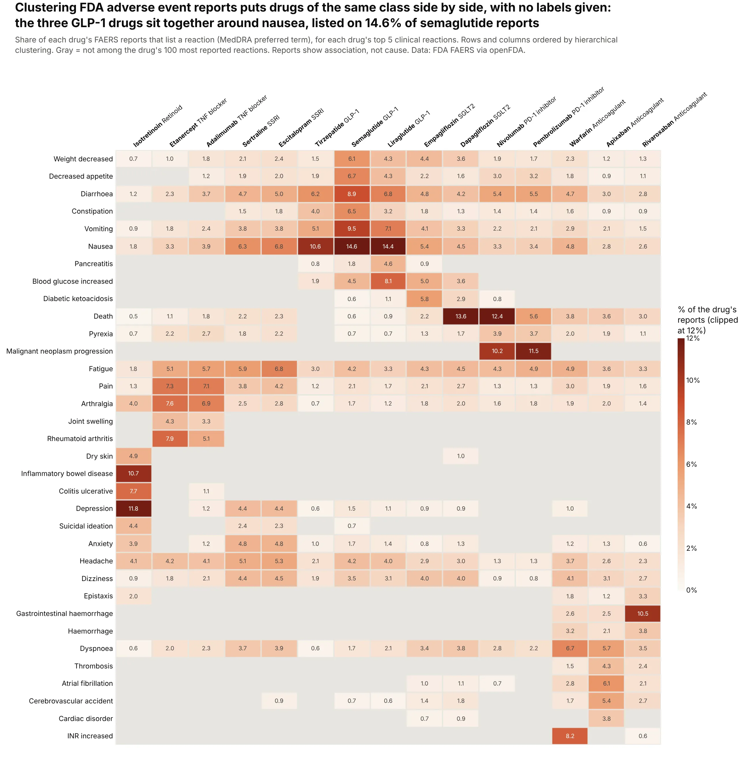
A two-way table of counts. Clustering 15 drugs on their adverse event reports alone puts drugs of the same class side by side, with the three GLP-1 drugs around nausea (14.6% of semaglutide reports); a report shows that a reaction was reported, not that the drug caused it. Data: FDA Adverse Event Reporting System (FAERS) via openFDA.

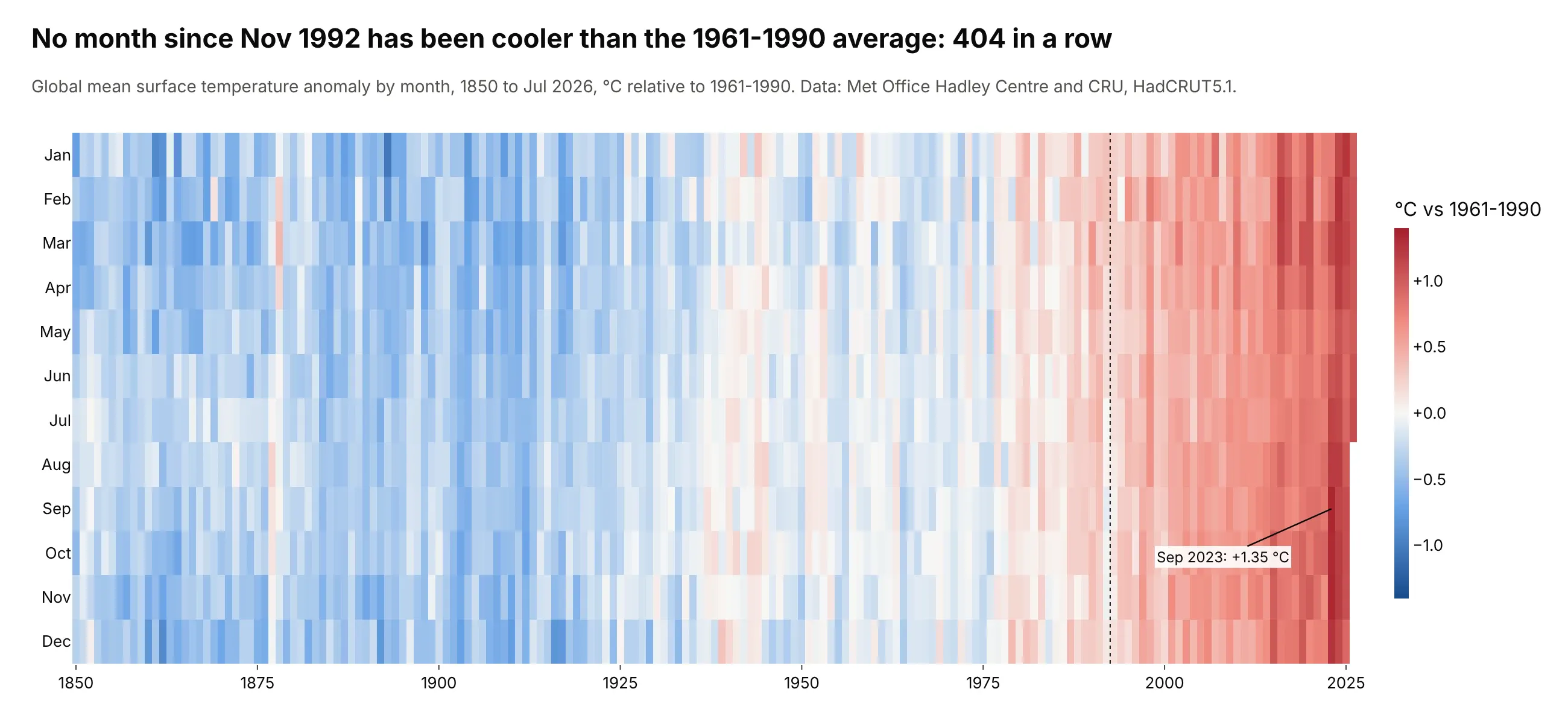
A long time series folded into month x year. No month since November 1992 has been cooler than the 1961-1990 average, 404 in a row, and September 2023 was the warmest at +1.35 °C. Data: Met Office Hadley Centre and CRU, HadCRUT5.1 (Morice et al. 2021).

A short history

Shaded tables are older than computers: Leland Wilkinson and Michael Friendly's history of the cluster heat map (2009) traces them to Toussaint Loua's 1873 shaded table of statistics for the districts of Paris. In the 1960s, Jacques Bertin drew tables as black and white cells and physically rearranged the rows and columns until groups appeared, which is the idea behind every clustered heatmap. Here is his townships example, redrawn with Plotly:

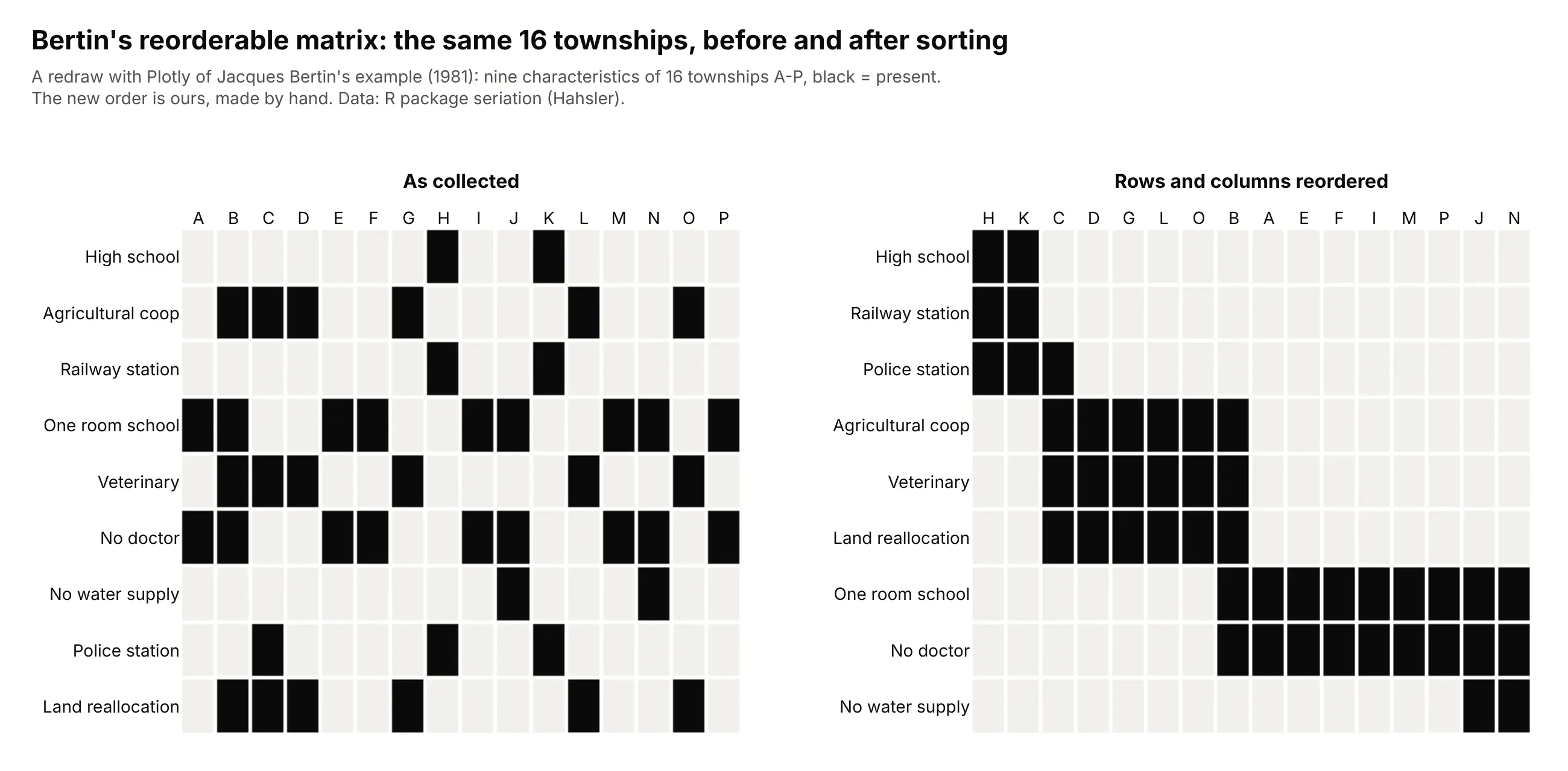
According to Wilkinson and Friendly, the term "heat map" was trademarked in 1991 for a display of financial market data, and the clustered heatmap became standard in biology after Eisen and colleagues used it for gene expression in 1998.

Alternatives to a heatmap

Here's the same table of Texas electricity demand by weekday and hour drawn six ways. Some are better for the question, some worse, some just different:

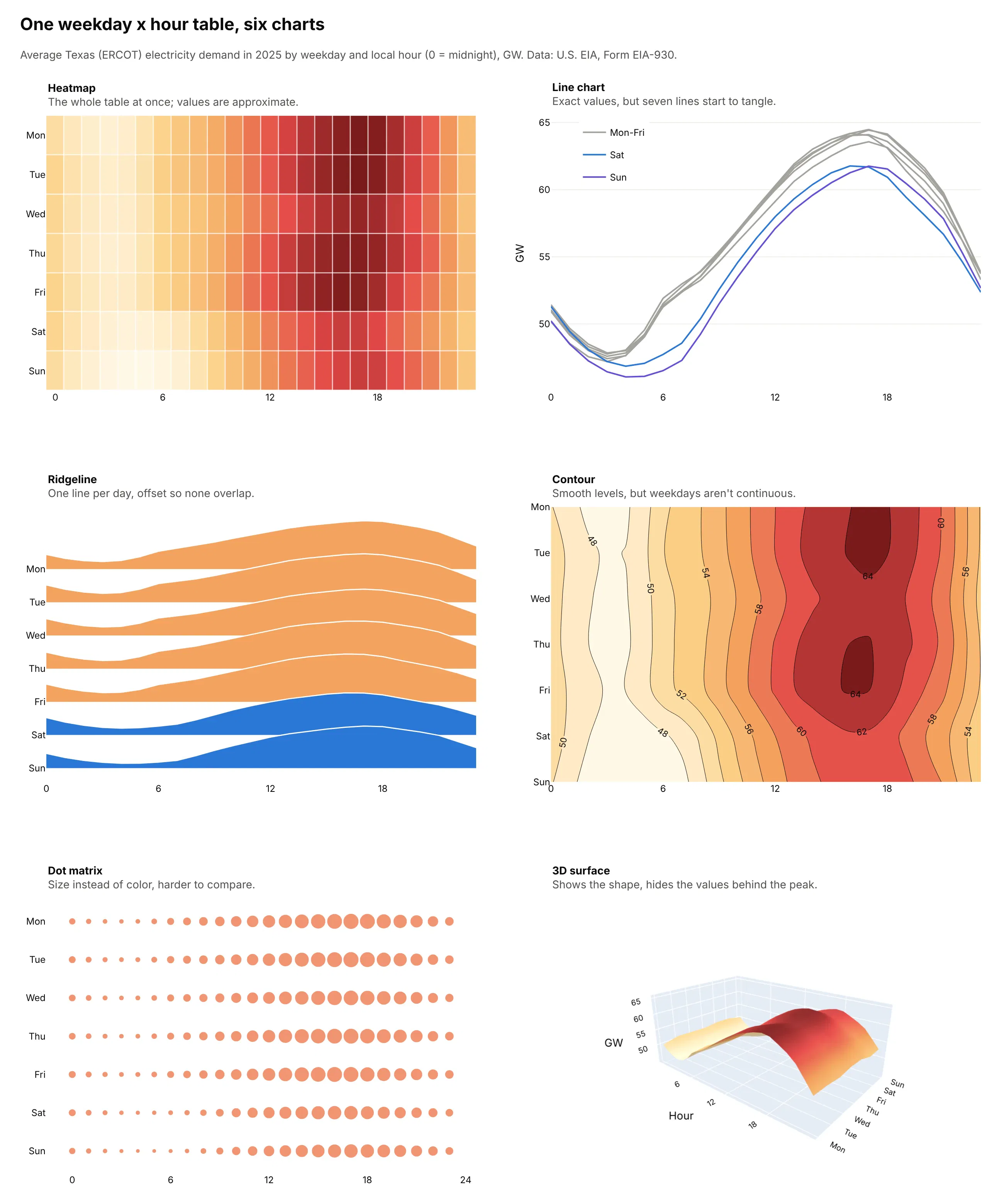
• Line chart (better for exact values of a few rows). People read position on a common scale more precisely than color, as Cleveland and McGill (1984) measured, so the line chart shows clearly that Saturday and Sunday run below the weekdays from early morning until the evening peak. With seven lines it starts to tangle, and with 52 weeks or 50 states it stops working.
• Ridgeline plot (works too, for a dozen rows or fewer). One curve per row, offset so they don't overlap, keeps the shape of each row readable. See our ridgeline plot guide.
• Contour plot (worse for categories). It interpolates between cells, which only makes sense when both axes are continuous; here it draws levels between Friday and Saturday that don't exist. For a continuous field it's the better chart. See our contour plot guide.
• Dot matrix (worse). Circle size is harder to compare than color, and the difference between 46 and 64 GW is hard to see.
• 3D surface (different). It shows the overall shape, a ridge from the afternoon peak of 64.5 GW down to 46.1 GW at 4 am on Sunday, but hides cells behind the peak and makes values hard to read.

For one value per day laid out like a wall calendar, see our calendar heatmap guide.

How to make a heatmap

With AI

ChatGPT, Claude Code, GitHub Copilot, Cursor and other AI tools are excellent at writing Plotly code. Name Plotly in the prompt, describe the rows, columns and color, and list the checks you want:

With Plotly Studio

Plotly Studio is a desktop app where you point an AI at a dataset and it builds charts and a Dash app around your questions. Ask for a heatmap the same way:

Show a correlation heatmap of daily returns for the tickers in this file, ordered by hierarchical clustering, lower triangle only, with the value in each cell and a blue-white-red scale fixed at -1 to 1 with white at zero. Add a date range slider that recomputes the correlations.

Make a heatmap in Python or JavaScript

This is the code AI tools write under the hood. In Python, px.imshow takes a DataFrame or 2-D array and uses its index and columns as labels:

In JavaScript, plotly.js takes z as an array of rows, plus the x and y labels:

For point data, px.density_heatmap(df, x="lon", y="lat", nbinsx=100, nbinsy=60) counts points in bins, and z="outcome", histfunc="avg" maps the average of a column instead.

Share it

Every Plotly chart has a Share chart button (the cloud icon in its toolbar) that uploads it to Plotly Cloud and gives you a link. Only you can see it until you change its visibility.

For a live app, put the chart in a Dash app and publish it with the Plotly Cloud CLI. Coding agents can run these commands for you:

If your data has to stay in your own cloud or data center, publish to Dash Enterprise instead.

Dos and don'ts

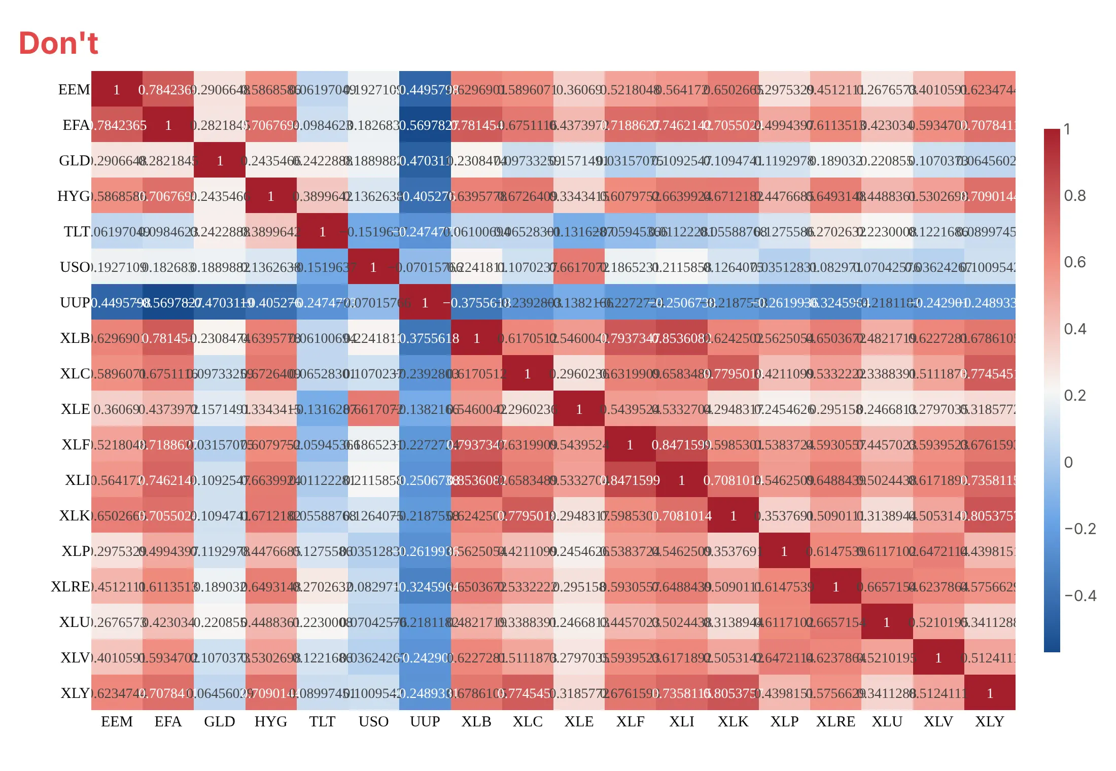
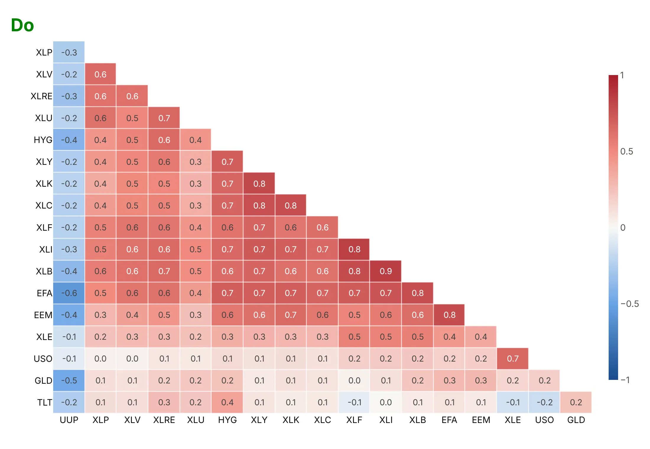
Plotly keeps the rows in the order of your data and stretches the color scale from the minimum to the maximum unless you tell it otherwise. For a correlation matrix, that means alphabetical tickers and a scale where white isn't zero. Here is the same matrix of 18 asset ETFs both ways, with the same blue-white-red colors.

Don't sort rows alphabetically, let the color range follow the data (here white lands near 0.2 instead of zero), draw both halves of a symmetric matrix with its diagonal of 1s, or print raw unformatted values that overflow the cells:

Do order rows and columns by clustering, fix the scale at -1 to 1 with white at zero, show one triangle without the diagonal and print the values with one decimal:

Pick the color scale for the data

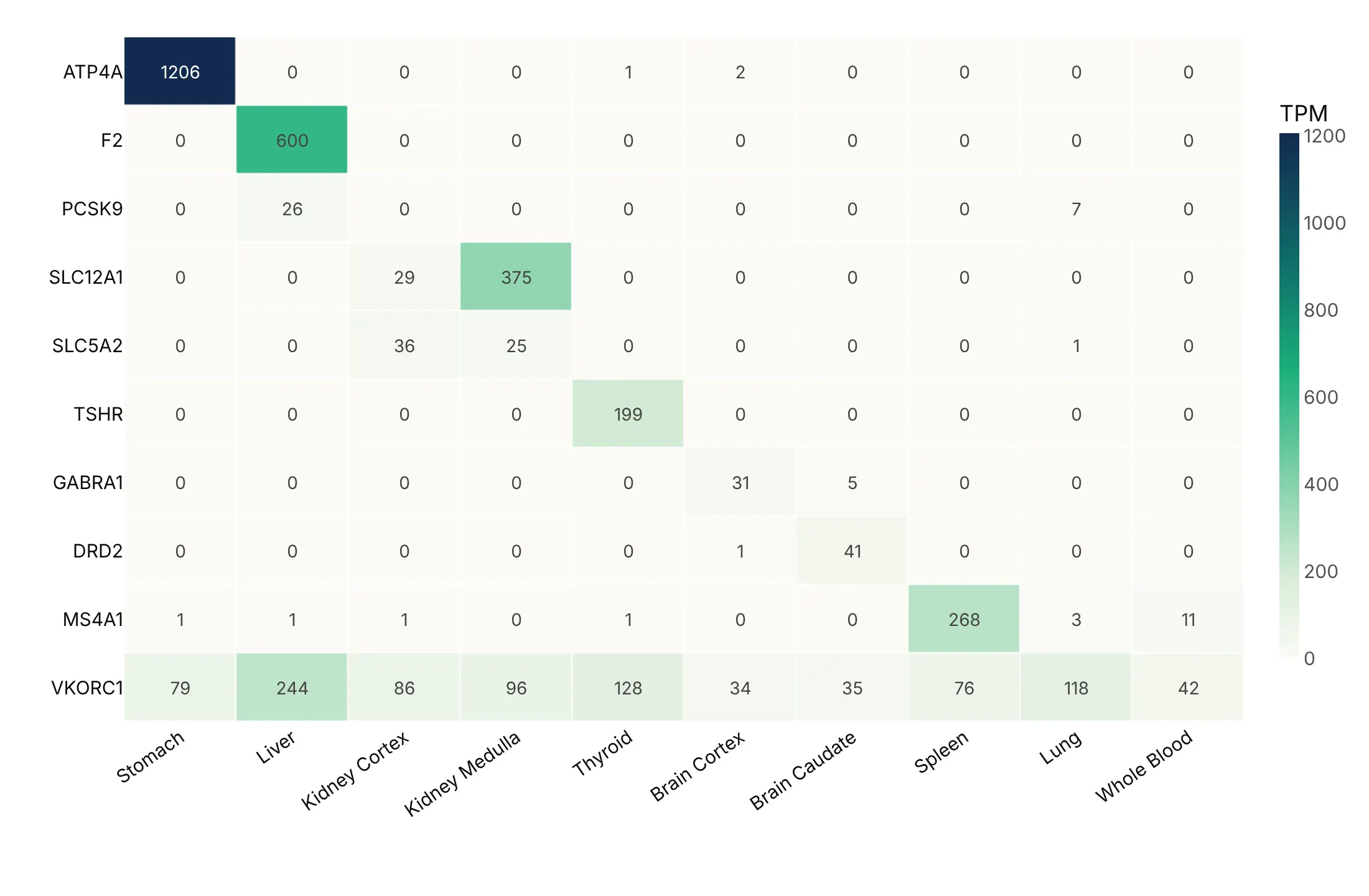
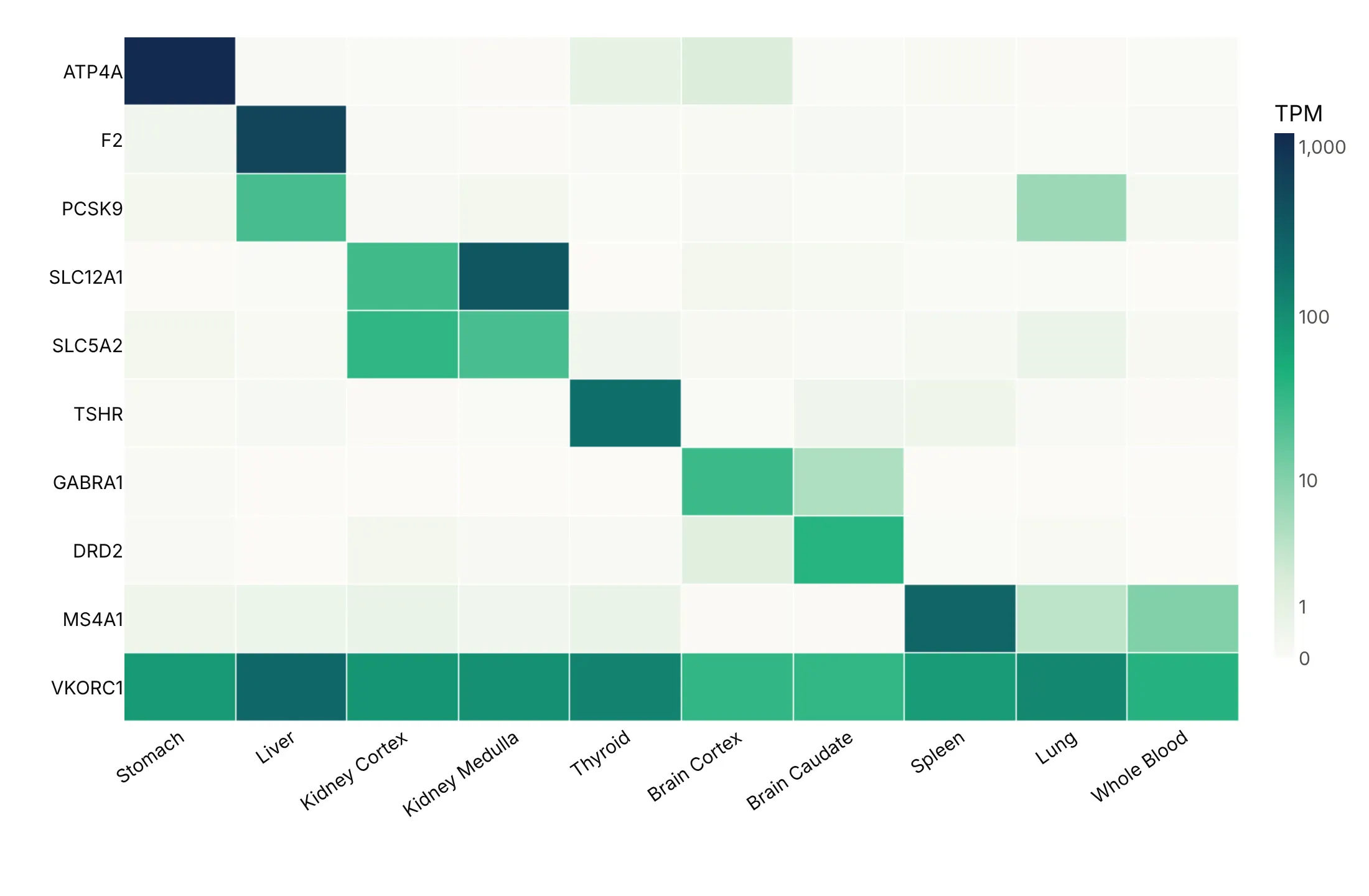
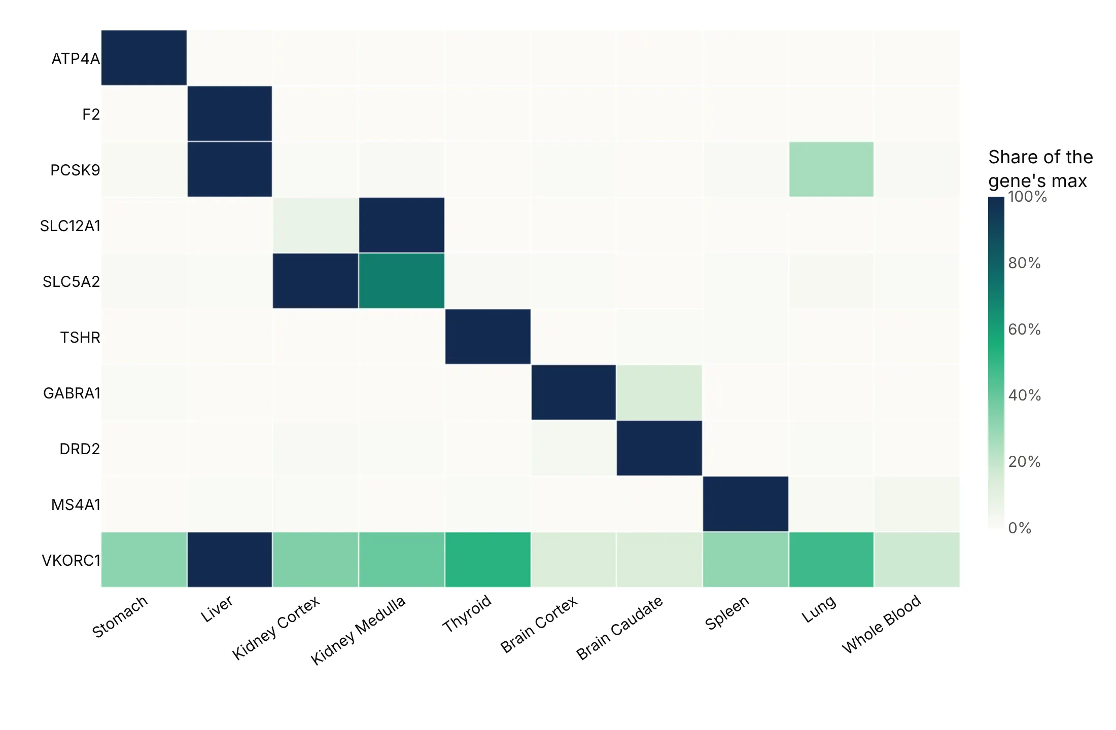
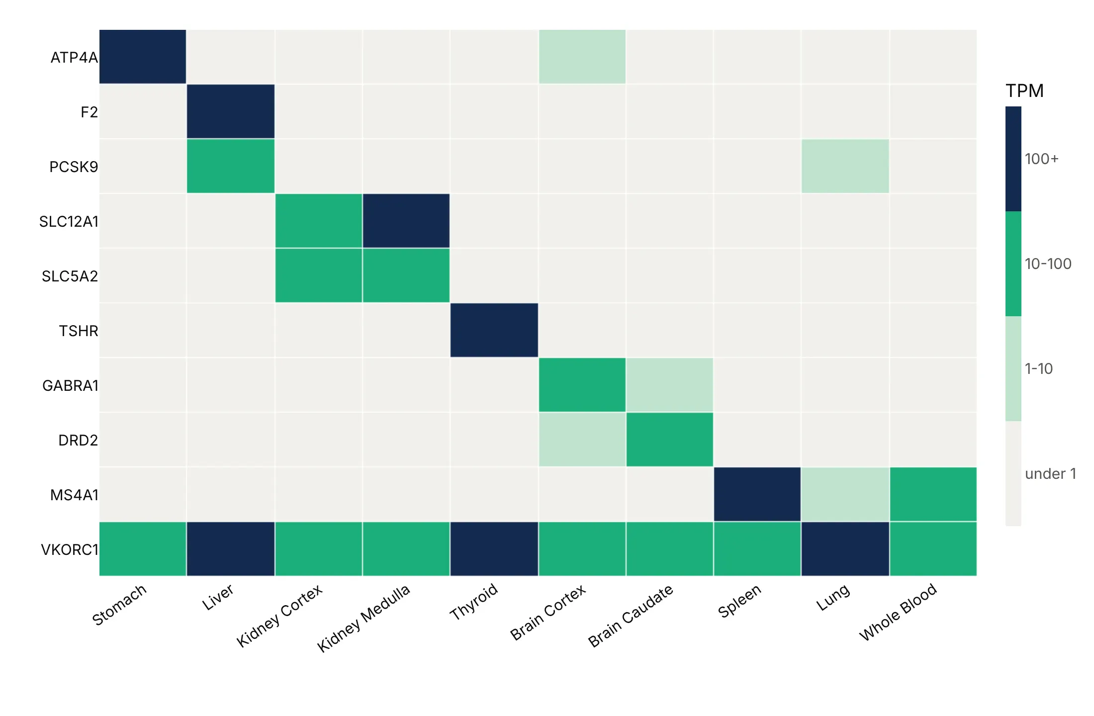
The color scale changes what readers see. Here is one table four ways: the median expression of 10 drug-target genes in 10 human tissues, from GTEx, in transcripts per million (TPM).

Linear (avoid when one value dominates). The stomach's proton pump, ATP4A at 1,206 TPM, sets the top of the scale, so most other cells look the same pale color.

Log. Coloring by log10(TPM + 1), with the colorbar labeled in TPM, shows every gene's pattern, including VKORC1, warfarin's target, which is expressed in every tissue.

Scaled per row. Dividing each gene by its own highest tissue shows where each gene peaks, at the cost of no longer showing how much it is expressed.

Binned. Four levels (under 1, 1-10, 10-100 and 100+ TPM) drawn with a stepped colorscale read like a table of thresholds.

Checklist

Do

• Write a title that states the takeaway.
• Use a sequential scale for amounts, a diverging scale with zmid for values around a center (zero correlation, zero return, a long-run average), a log scale for data spanning orders of magnitude and a stepped scale for thresholds.
• Fix the limits with zmin and zmax when the range has a meaning (-1 to 1 for correlations, 0 to 100% for shares), and clip outliers so ordinary cells still get color.
• Order rows and columns by a value, by time or by clustering (scipy.cluster.hierarchy).
• Print values in small grids with texttemplate="%{z:.1f}" (or text_auto in px.imshow).
• Leave missing cells as NaN over a gray plot_bgcolor, set hoverongaps=False, and say what gray means.

Don't

• Use a rainbow scale like Jet, which creates bands that aren't in the data and isn't readable by many colorblind readers (Borland and Taylor, 2007).
• Fill missing values with zero, because a zero is a measurement and a gap is not.
• Let one outlier set the scale for the other 99% of cells.
• Smooth a categorical grid with zsmooth or a contour plot, which invents values between Monday and Tuesday or between two countries.

Options to customize

These are the options that matter most in go.Heatmap, px.imshow and px.density_heatmap. The full list is in the Plotly heatmap documentation.

1. z, x, y: the values (a 2-D array of rows) and the column and row labels.
2. colorscale: a named scale or a list of [position, color] stops; repeat stops for a stepped (binned) scale.
3. zmin, zmax, zmid: fix the color limits, clip outliers and center a diverging scale.
4. coloraxis (layout): share one color scale between traces, subplots or facets.
5. texttemplate, textfont: print values in cells, for example "%{z:.1f}", in grids of up to a few hundred cells.
6. xgap, ygap: pixels between cells, 1-3 px for small grids.
7. hoverongaps: set to False so NaN cells don't show a hover label.
8. connectgaps: fills NaN by interpolation; rarely what you want, because it invents values.
9. zsmooth: "best" or "fast" smoothing, for continuous fields only.
10. customdata, hovertemplate: show the raw value in the hover when the color is transformed (log, per row).
11. colorbar (tickvals, ticktext, orientation): relabel ticks for log or binned scales and place the colorbar.
12. xaxis.type="category", yaxis.autorange="reversed": equal-width cells and the first row on top, for tables.
13. px.imshow(text_auto=, aspect=, facet_col=): an annotated heatmap from a DataFrame or array, and small multiples from a 3-D array.
14. px.imshow(color_continuous_midpoint=): center a diverging scale in Plotly Express.
15. px.density_heatmap(nbinsx=, nbinsy=, histfunc=, histnorm=): bin point data and count, sum or average it; go.Histogram2d does the same as a trace.

More heatmap examples

Ten more heatmaps built from real public data, each with its source, the technique that makes it work and a prompt to rebuild it.

1. The US Treasury yield curve since 1990

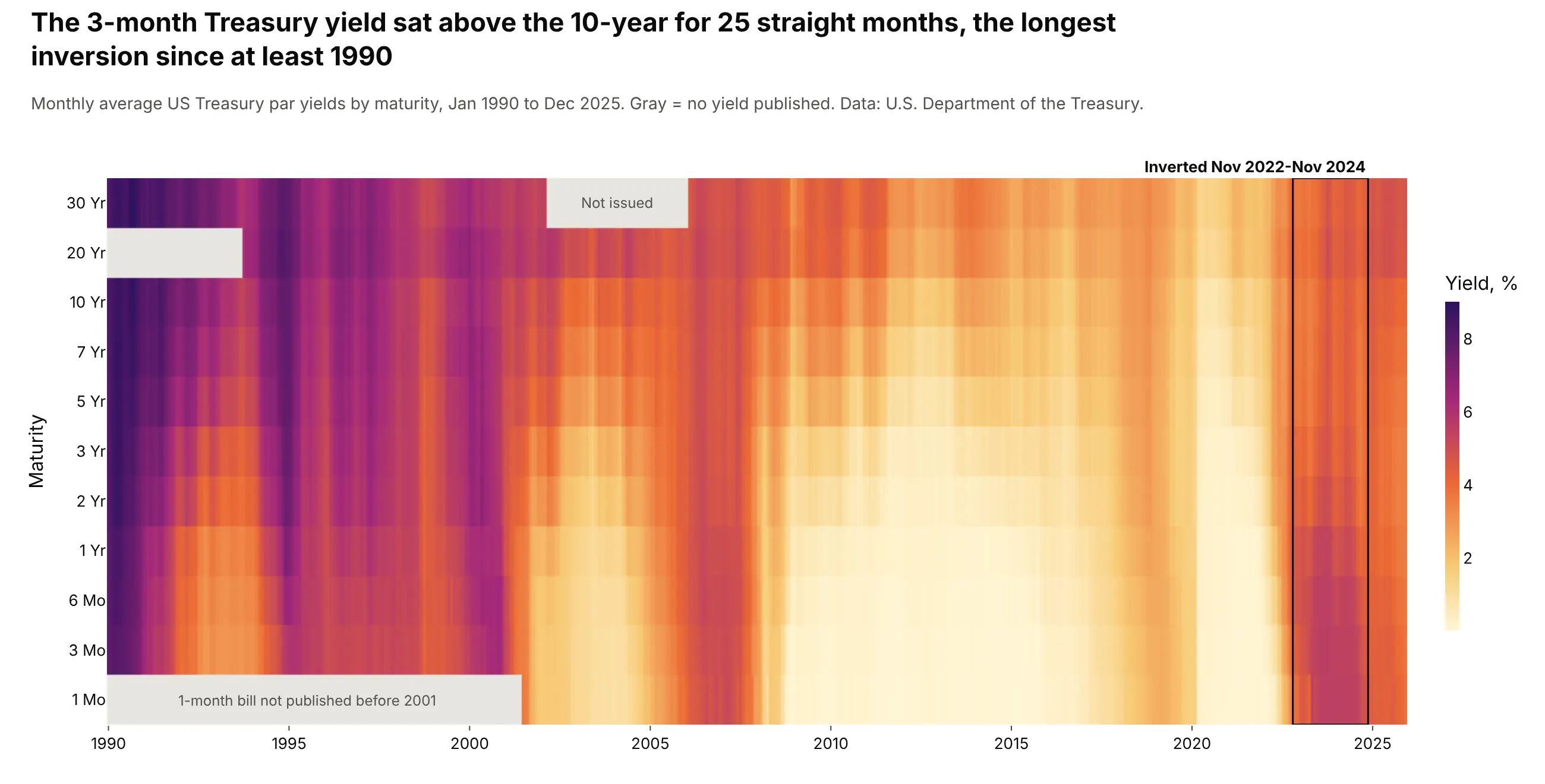
Each column is one month's yield curve, so rate cycles are vertical bands and an inverted curve is a column that gets lighter from short to long maturities. The 3-month yield sat above the 10-year for 25 straight months from November 2022, the longest run since at least 1990. Data: U.S. Department of the Treasury, Daily Treasury Par Yield Curve Rates.

Tip: set plot_bgcolor to gray so maturities the Treasury didn't publish (the 30-year from 2002 to 2006) read as missing, not as low.

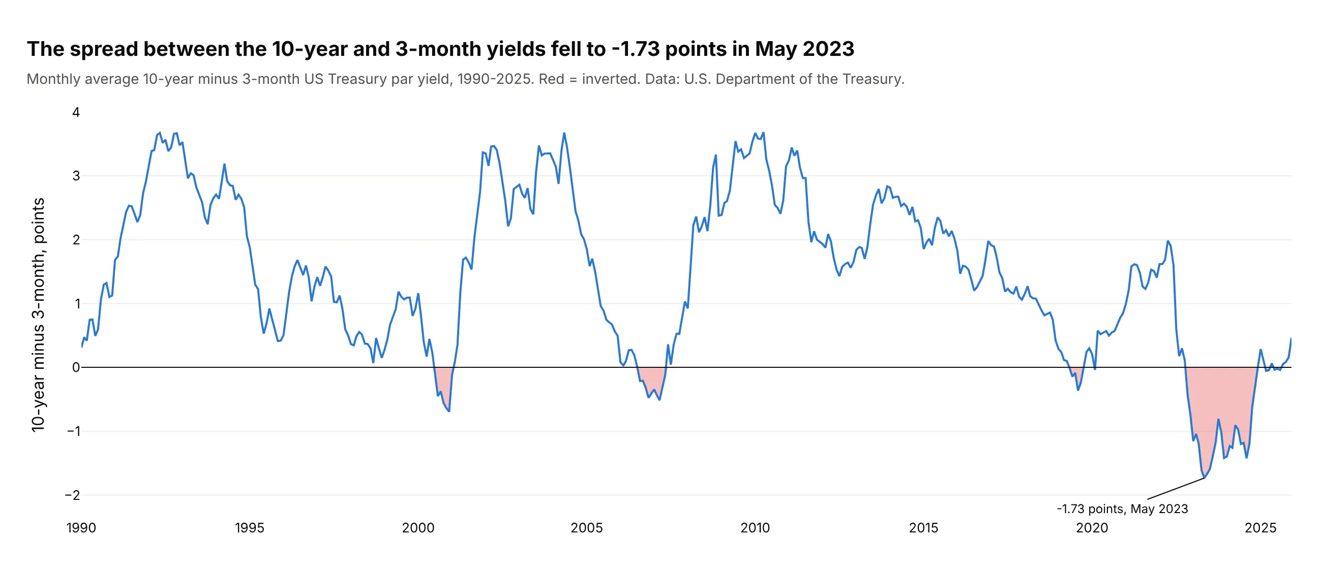
Another way to see it: the 10-year minus 3-month spread as a single line shows the depth of each inversion, down to -1.73 points in May 2023.

2. S&P 500 monthly returns, 1986-2025

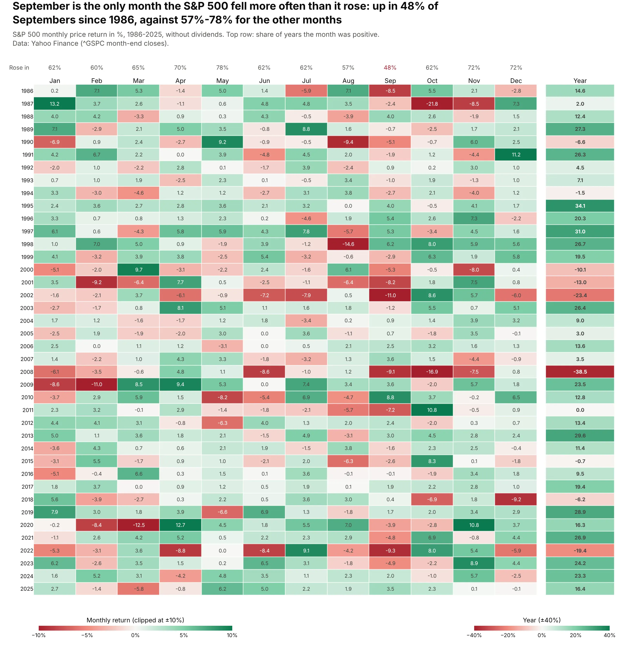
This is the monthly returns table that fund factsheets print. Over 480 months the S&P 500 rose 64% of the time, but September rose in only 48% of years, the only month below half; October 1987 is the darkest cell at -21.8%. Data: Yahoo Finance, S&P 500 index month-end closes (price return), 1986-2025.

Tip: give the yearly column its own coloraxis, because yearly returns are about three times larger than monthly ones.

3. Inflation in the G20 since 2000

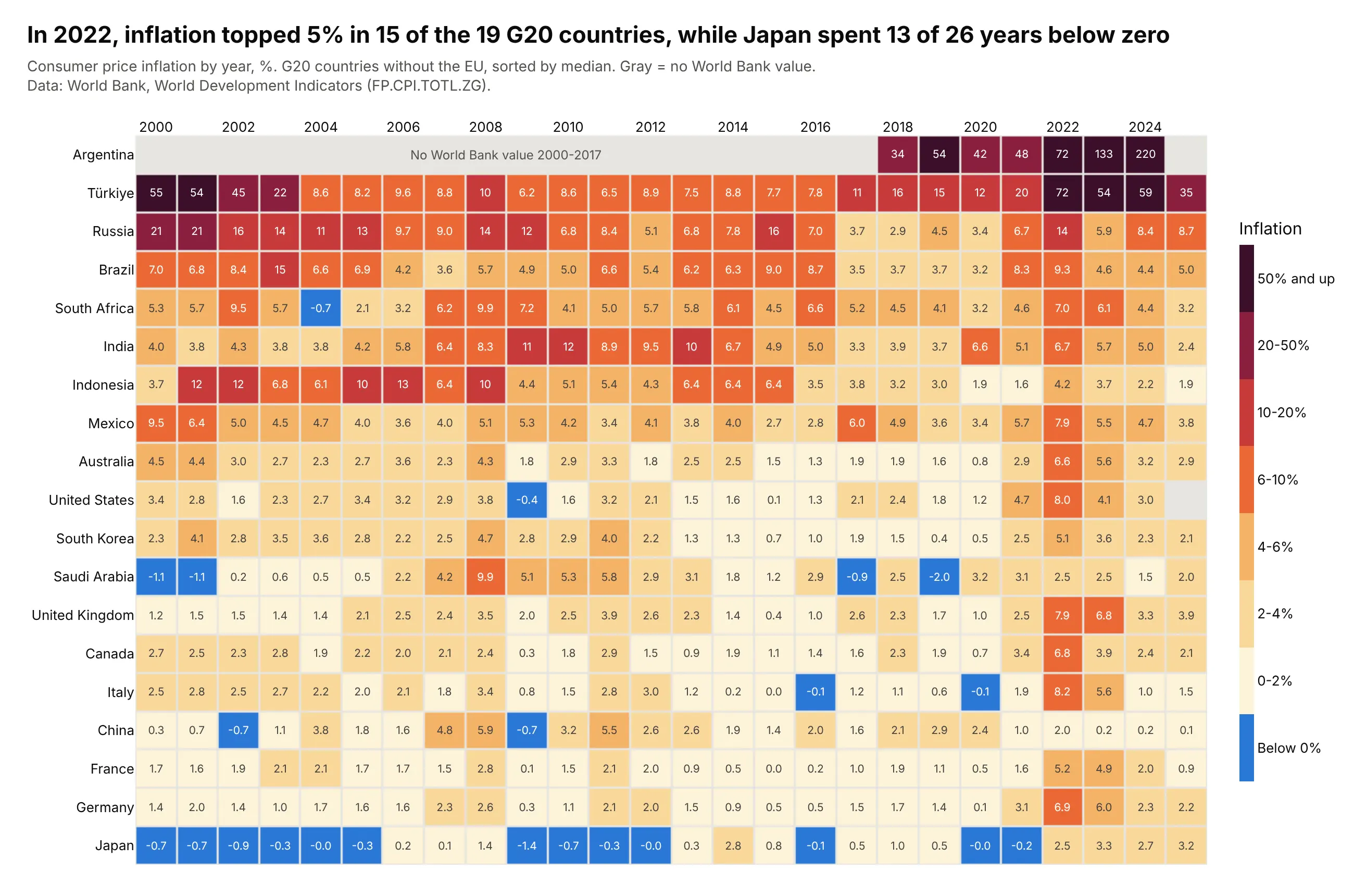
In 2022, inflation passed 5% in 15 of the 19 G20 countries, which shows up as one dark column. Japan's row is blue for 13 of 26 years, and the World Bank has no value for Argentina before 2018, which stays gray rather than looking like zero. Data: World Bank, World Development Indicators (FP.CPI.TOTL.ZG), 2000-2025.

Tip: for data from -2% to 220%, map values to bins with np.digitize and draw them with a stepped colorscale (two stops per color).

4. Seven US grids, one shared scale

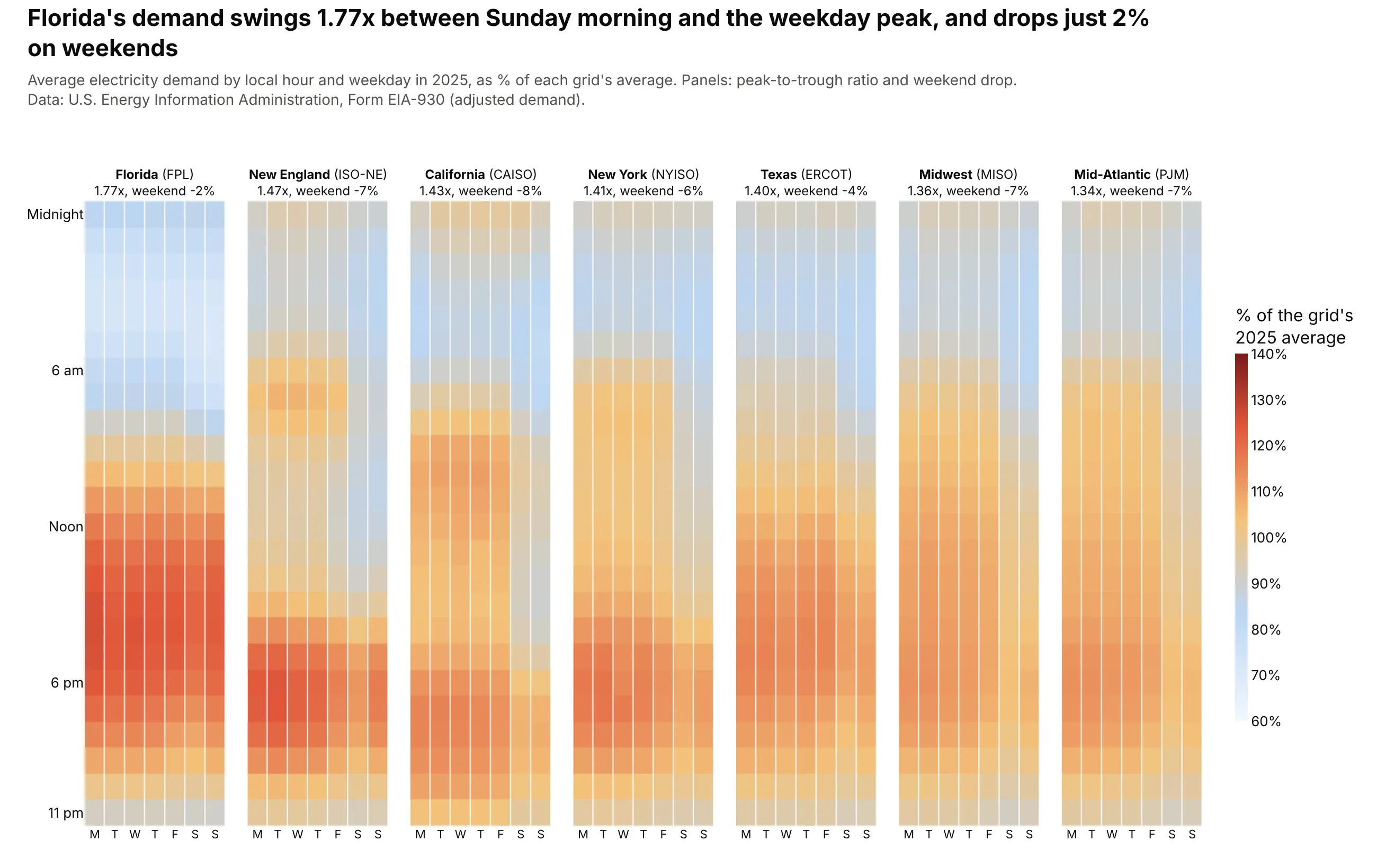
Dividing each grid's demand by its own average lets grids of very different size share one scale. Florida's demand swings 1.77 times from Sunday morning to the weekday peak, the most of the seven, and drops only 2% on weekends, against 7% in New England. Data: U.S. EIA, Form EIA-930, adjusted demand, 2025.

Tip: pass a 3-D array to px.imshow with facet_col=0 to get small multiples with one color axis.

5. Coal's share of electricity, 2000-2024

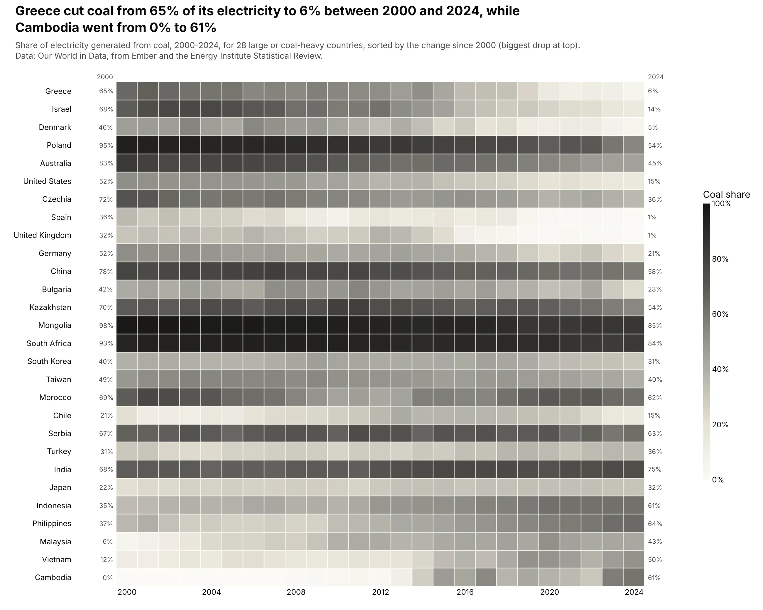
Sorting the rows by the change from 2000 to 2024 turns the table into two triangles. Greece cut coal from 65% of its electricity to 6% and the UK from 32% to 1%, while Cambodia went from 0% to 61% and Vietnam from 12% to 50%. Data: Our World in Data, from Ember and the Energy Institute Statistical Review.

Tip: sort rows by a summary of each row (here the change) before you reach for clustering; it's simpler and easy to explain in the subtitle.

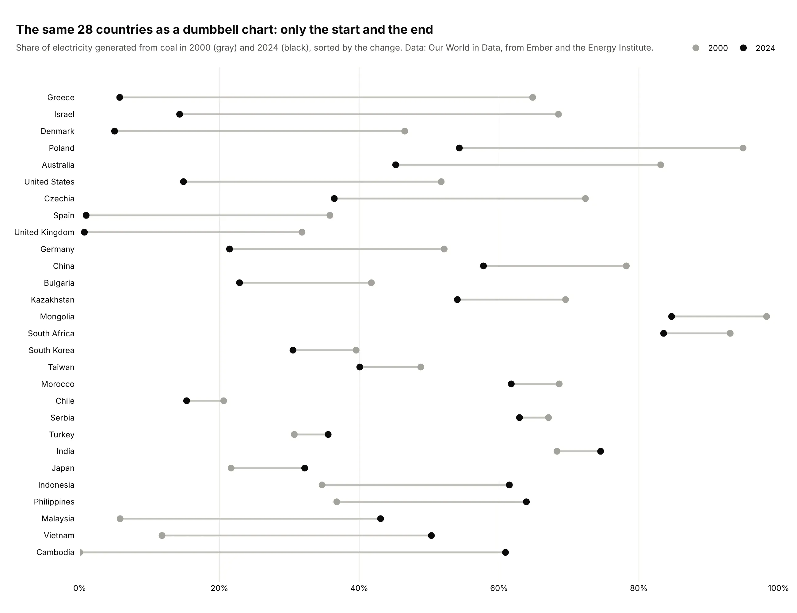
Another way to see it: a dumbbell chart shows only the first and last year, which makes the size of each change easier to compare but hides when it happened.

6. Offshore drilling in the Gulf

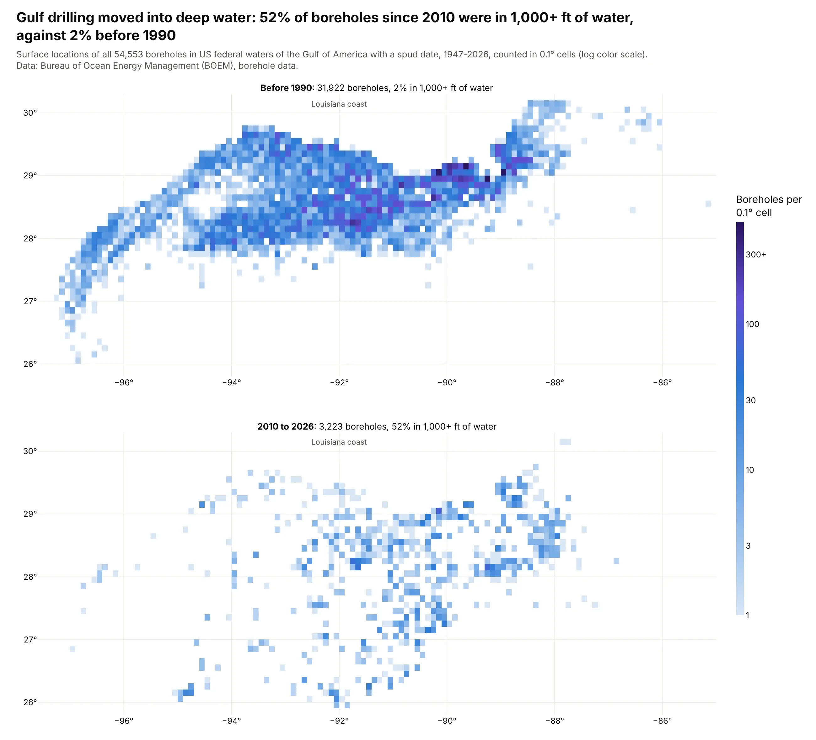
A scatter of 54,553 boreholes is one solid blob, so we count them in 0.1° cells instead. Before 1990, 2% of boreholes were drilled in more than 1,000 ft of water; since 2010, 52% were, and the map shifts south off the shelf. Data: Bureau of Ocean Energy Management (BOEM), borehole data, 1947-2026.

Tip: color by log10(count) and relabel the colorbar ticks with real counts (1, 3, 10, 30, 100, 300).

7. Where drug targets are expressed

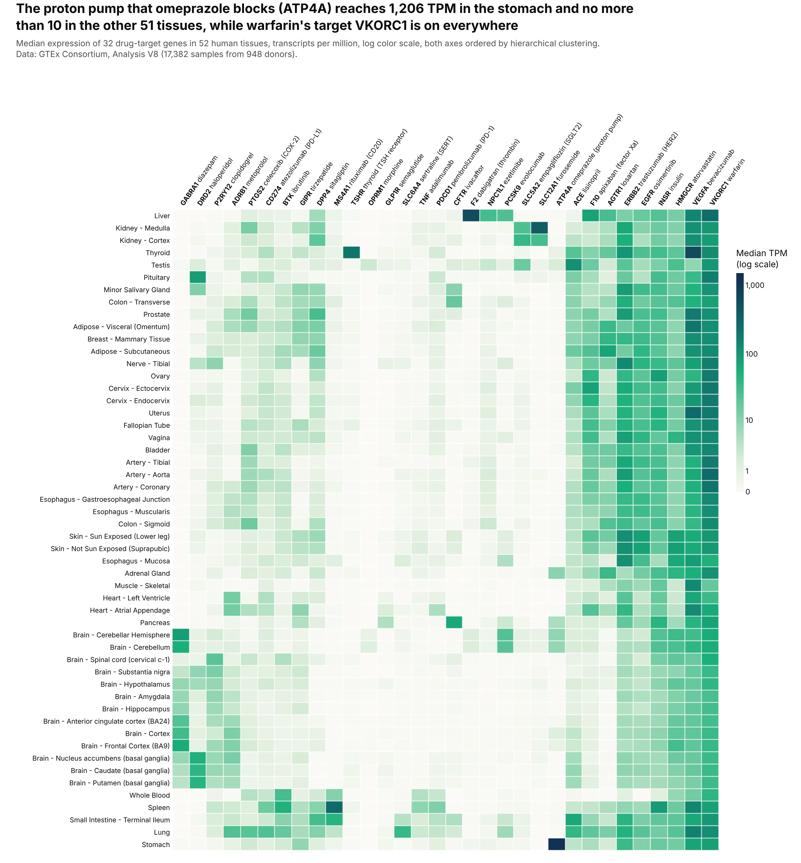
Expression runs from zero to over 1,000 TPM, so a log scale is the only way to see every gene. The proton pump that omeprazole blocks (ATP4A) reaches 1,206 TPM in the stomach and no more than 10 in any other tissue, while warfarin's target VKORC1 is above 17 TPM everywhere. Data: GTEx Consortium, Analysis V8 (17,382 samples from 948 donors, Science 2020).

Tip: color by log10(TPM + 1) and set colorbar.tickvals to the logs of 1, 10, 100 and 1,000 with ticktext in TPM.

8. How often US senators vote together

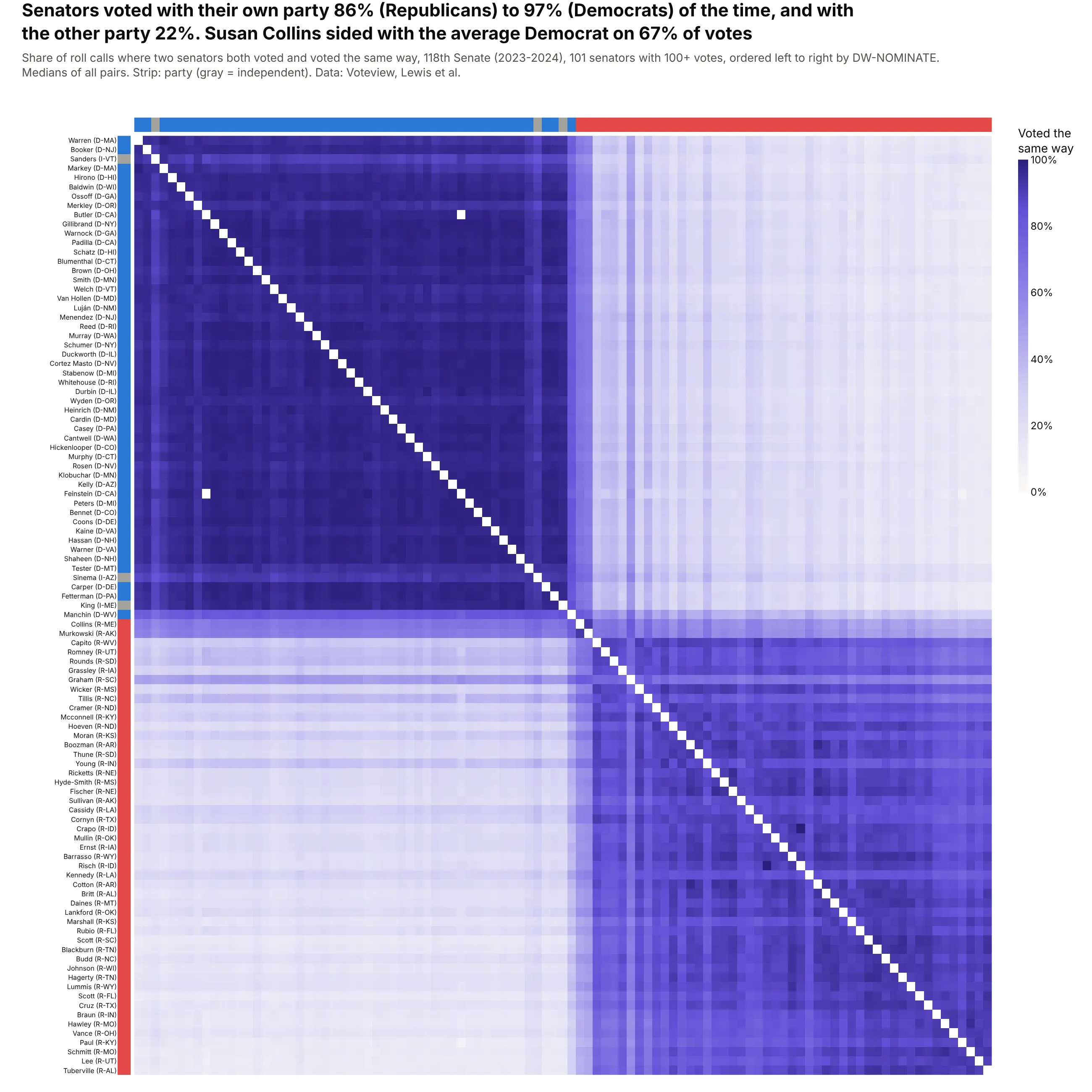
Ordered by each senator's left-right score, 10,201 pairs form two blocks: senators voted with their own party 86% (Republicans) to 97% (Democrats) of the time and with the other party 22%. Collins sided with the average Democrat on 67% of votes. Data: Voteview, 691 roll calls of the 118th US Senate, 2023-2024.

Tip: when you have a known 1-D score (here DW-NOMINATE), sort by it instead of clustering; the order is stable and easy to explain.

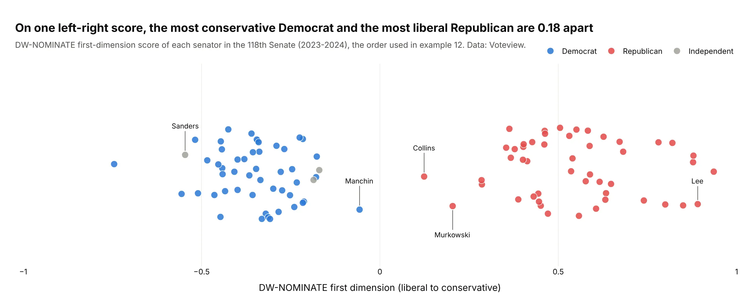
Another way to see it: the NOMINATE scores themselves, one dot per senator, show the gap the heatmap's blocks come from: 0.18 between the most conservative Democrat and the most liberal Republican.

9. Net migration between US states

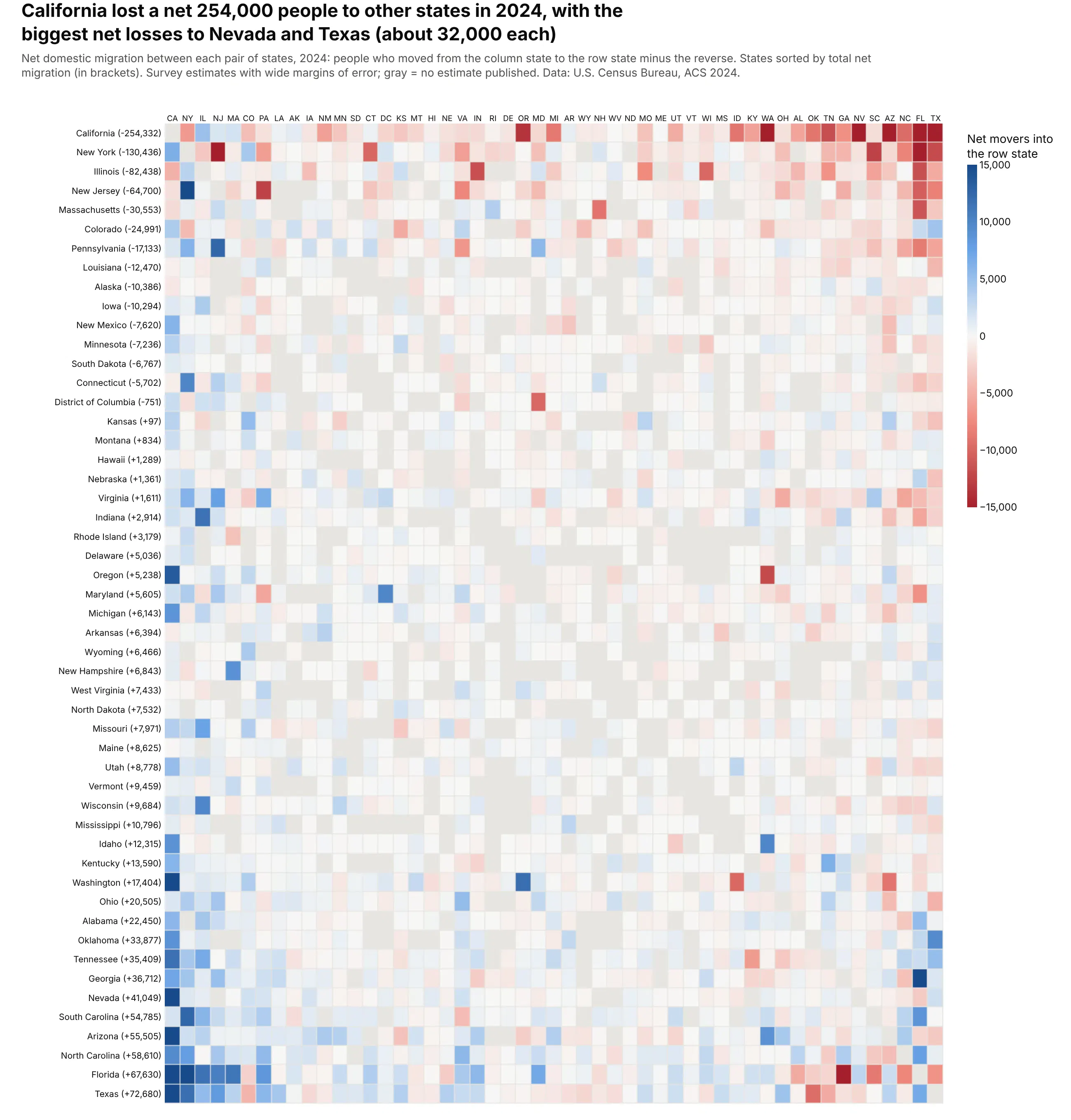
Net flows make the matrix antisymmetric, and sorting states by total net migration puts the losers on top and the gainers at the bottom. California lost a net 254,000 people to other states in 2024, with the biggest net losses to Nevada and Texas, about 32,000 each. These are survey estimates with wide margins of error. Data: U.S. Census Bureau, State-to-State Migration Flows 2024 (ACS 1-year).

Tip: use the same order on both axes, so the matrix reads as a mirror around the diagonal.

10. The strike zone umpires actually call

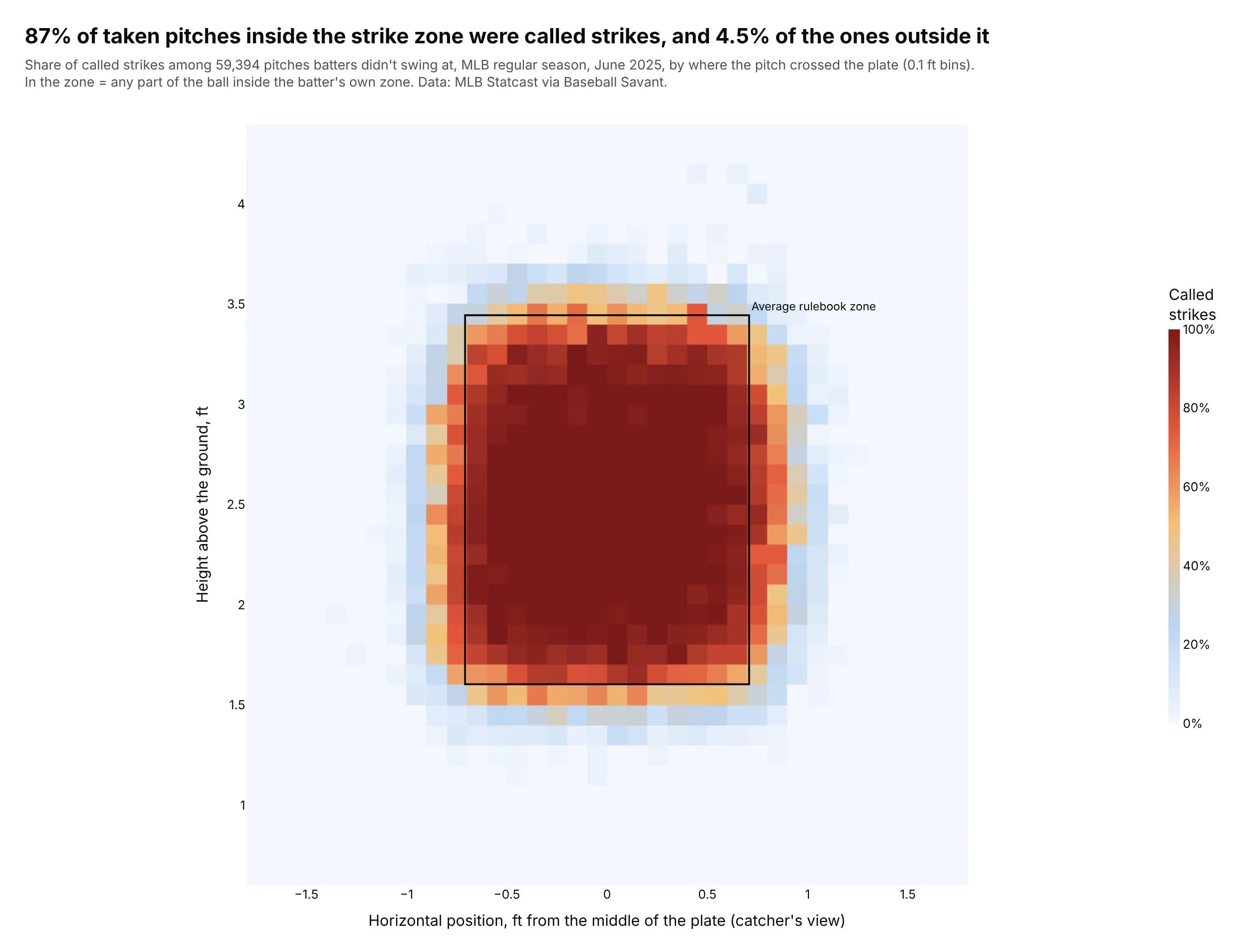
Averaging a 0/1 outcome in small bins turns 59,394 pitches into a probability map. 87% of taken pitches inside the rulebook zone were called strikes and 4.5% of those outside it, and the edges show where umpires disagree with the rectangle. Data: MLB Statcast via Baseball Savant, June 2025.

Tip: px.density_heatmap(df, x=..., y=..., z="called_strike", histfunc="avg") maps a binned mean instead of a count.