
Chris Parmer
November 15, 2026
Waterfall Plots for Tumor Response - A Complete Guide
TL;DR
- A tumor waterfall plot draws one bar per patient for the best percent change in the size of their tumors compared with the start of treatment, sorted from the largest growth on the left to the largest shrinkage on the right, with dashed lines at the RECIST (Response Evaluation Criteria in Solid Tumors) cut-offs of +20% for progressive disease and -30% for a partial response.
- Tumor waterfall plots are also known as waterfall charts in oncology trials, and are similar to sorted bar charts, swimmer plots, and spider plots, which show the same percent change as one line per patient over time.
- Oncologists and clinical data scientists use them in early-phase trials to see how deep each patient's response was, which cancer types or biomarkers the shrinkage comes from, and whether a drug shrinks tumors at all before a larger trial.
- You can make one with Plotly from a go.Bar trace, one bar per patient, plus dashed lines with add_hline, and a spider plot from one go.Scatter line per patient. Short helper functions are below.
This is not the financial waterfall chart. The financial one, which Plotly draws with go.Waterfall, shows how a starting value turns into an ending value through a series of increases and decreases, and has its own guide: Waterfall Charts - A Complete Guide. The tumor waterfall plot in this guide shares the name because the sorted bars look like a cascade, and nothing else: its bars start at zero, each one is a different patient, and the heights are not added up.
What is a tumor waterfall plot?
Tumor waterfall plots look like this:
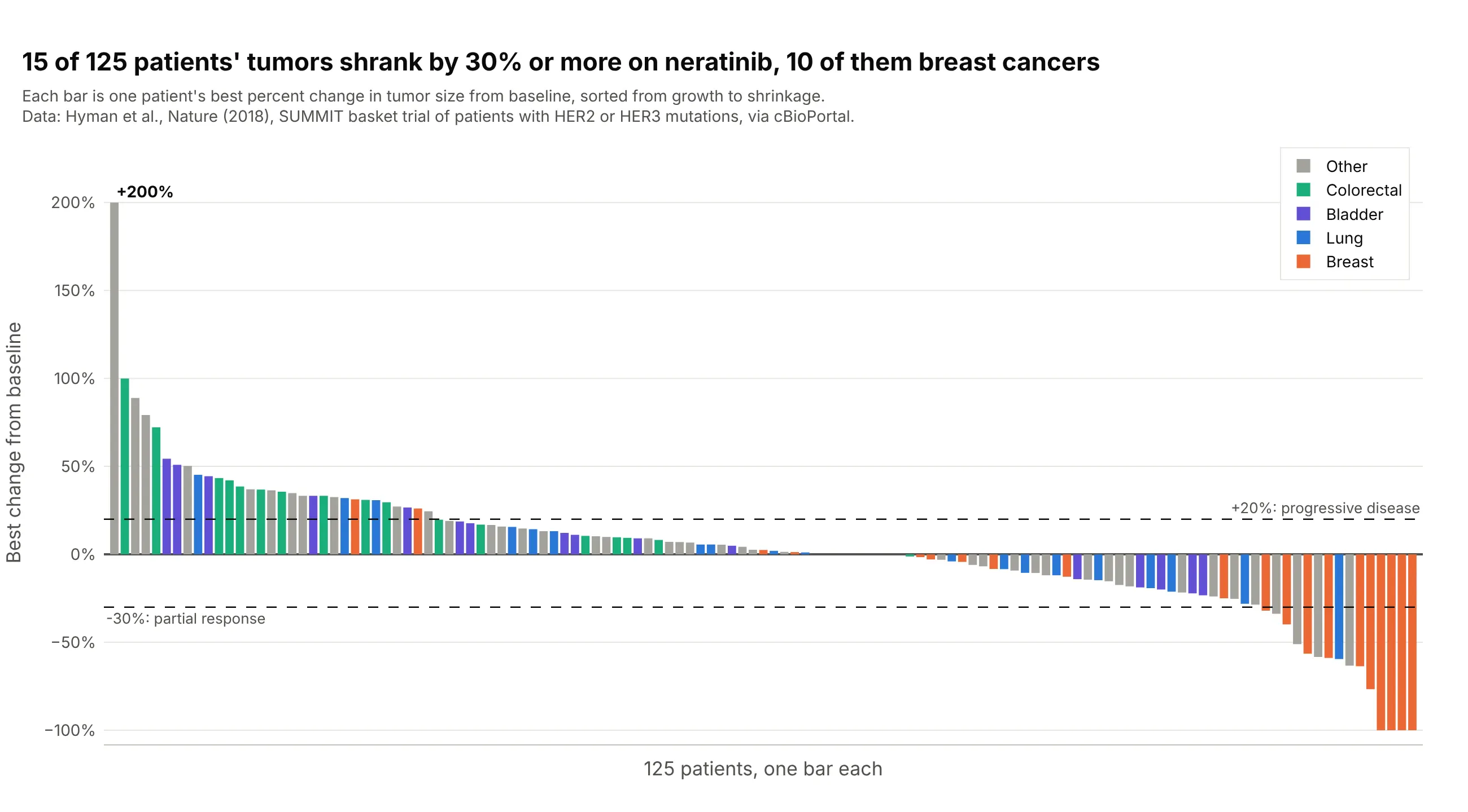
Data: Hyman et al. (2018), Nature, the SUMMIT trial of the drug neratinib in 125 patients with measurable tumors and mutations in the HER2 or HER3 genes (HER2 stands for human epidermal growth factor receptor 2), via cBioPortal.
How do you read a tumor waterfall plot? In the example above, notice these things:
- Each bar is one patient, and its height is the best percent change in the size of the patient's tumors (the sum of the diameters of up to five target lesions) at any scan, compared with the scan before treatment. The bars are sorted, so the patients who did worst are on the left and the patients who did best are on the right.
- Bars above zero are patients whose tumors grew, and bars below zero are patients whose tumors shrank. Thirty-one bars rise above the +20% line, and the first one, at +200%, is a tumor that tripled in size.
- Bars below the -30% line are partial responses by RECIST. Fifteen of the 125 patients got there, and four reached -100%, which means every measured tumor was gone.
- The colors show which cancer type each patient had. Ten of the 15 patients who passed -30% had breast cancer (10 of 21 breast cancer patients), while none of the 16 bladder cancer patients or 18 colorectal cancer patients did, so the drug looks active in some cancer types and not others.
- Seventy-nine patients sit between the two dashed lines, which RECIST calls stable disease.
It's often used for charts like these:
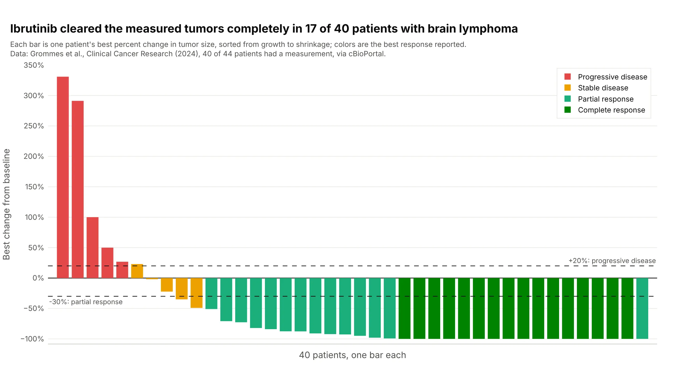
Depth of response in a blood cancer. Ibrutinib cleared the measured tumors completely (-100%) in 17 of 40 patients with lymphoma in the brain, and 32 of the 40 had shrinkage of 30% or more, so the bars pile up at the floor of the chart. Four more patients had no measurement and are left out. Data: Grommes et al. (2024), Clinical Cancer Research, via cBioPortal.
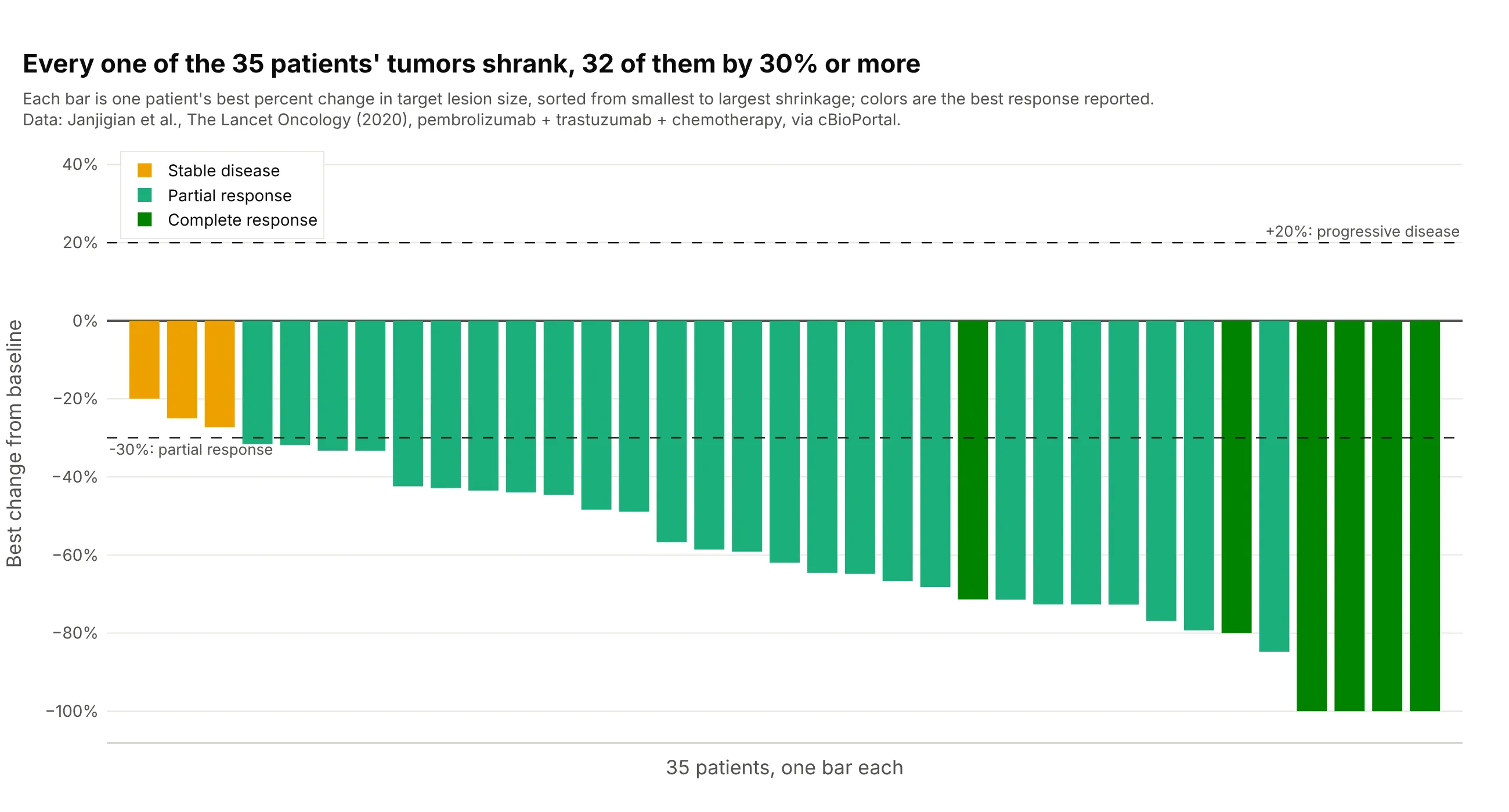
A combination in a first-line trial. All 35 measured patients with HER2-positive esophageal, stomach, or gastro-esophageal junction cancer had tumors that shrank on pembrolizumab, trastuzumab, and chemotherapy, 32 of them by 30% or more and four to -100%, with a median of -62%. Data: Janjigian et al. (2020), The Lancet Oncology, via cBioPortal.
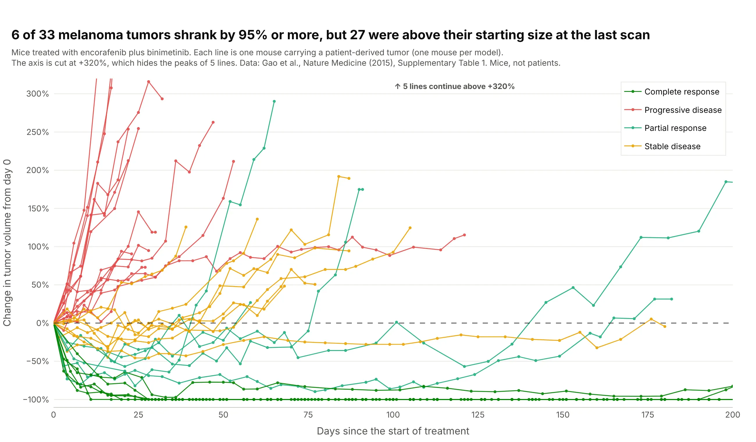
The spider plot, the waterfall plot over time. Each line is one mouse carrying a tumor from a patient's melanoma (a patient-derived xenograft, or PDX), as percent change in tumor volume since the first day of treatment. Six of 33 tumors shrank by 95% or more, and 27 were above their starting size at the last measurement, which a waterfall plot of the best change would hide. Data: Gao et al. (2015), Nature Medicine, Supplementary Table 1. These are mice, not patients, because we could not find scan-by-scan tumor measurements of real patients that anyone can download.
A short history
Tumor waterfall plots are a recent habit in oncology. By 2012, the Journal of the Advanced Practitioner in Oncology told nurses and other practitioners that waterfall plots "have begun to gain in popularity" for showing the results of trials, with one bar per patient sorted from worst to best (Gillespie 2012). The same year, at PharmaSUG, the pharmaceutical industry's conference for users of the SAS (Statistical Analysis System) language, Niraj Pandya wrote that the chart was "gaining recognition recently for the reporting of overall drug response in Oncology clinical trials" and showed the code to draw it, with the patients sorted from the worst value on the left to the best on the right and the bars colored by response category (Pandya 2012). One reason is that response categories throw information away, as Pandya's abstract puts it: two patients both reported as "stable disease" can have tumors that grew 15% or shrank 25%, and a waterfall plot shows the difference.
The spider plot followed as the answer to the main weakness of the waterfall plot, which is that it has no time axis. SAS's Sanjay Matange described it in 2016 as "another way of presenting the Change from Baseline for tumors for each subject in a study by week" (Matange 2016). A 2019 paper in Pharmaceutical Statistics then listed the waterfall plot's limits, that it masks the time dynamics of tumor size, often has an ambiguous y-axis label, and has a low data-to-ink ratio, and recommended spider plots with raw lesion measurements, which it calls spaghetti plots, next to them (Mercier et al. 2019). We did not find the underlying data of an early waterfall plot, so there is no redraw here, and every chart in this guide uses data we could download.
How tumor response is measured: RECIST in plain words
The dashed lines on a tumor waterfall plot come from RECIST, the Response Evaluation Criteria in Solid Tumors. RECIST 1.0 came out in 2000 (Therasse et al. 2000) and the current version, 1.1, in 2009 (Eisenhauer et al. 2009). It turns CT (computed tomography) or MRI (magnetic resonance imaging) scans into a few categories that every trial reports the same way.
At the start of treatment, a radiologist picks up to five measurable tumors, the target lesions, with at most two per organ, measures the longest diameter of each, and adds them up. Every later scan is compared with that sum (RECIST working group of the European Organisation for Research and Treatment of Cancer):
- Complete response (CR): every target lesion has disappeared (lymph nodes count as normal again below 10 mm across).
- Partial response (PR): the sum has shrunk by 30% or more from the start.
- Progressive disease (PD): the sum has grown by 20% or more from its smallest value on study, and by at least 5 mm, or a new tumor has appeared.
- Stable disease (SD): neither of the above.
The best percent change that a waterfall plot shows is the most negative change from the start of treatment over all scans, or the smallest increase for a patient whose tumors never shrank, for example (45 mm - 60 mm) / 60 mm = -25%. Because RECIST measures progression from the smallest sum so far, not from the start, a bar can sit below +20% for a patient who is reported as progressive disease, and a patient with a new tumor counts as progressive disease whatever their target lesions did. Here are 34 patients treated with nivolumab, an immunotherapy drug, in the RECIST zones:
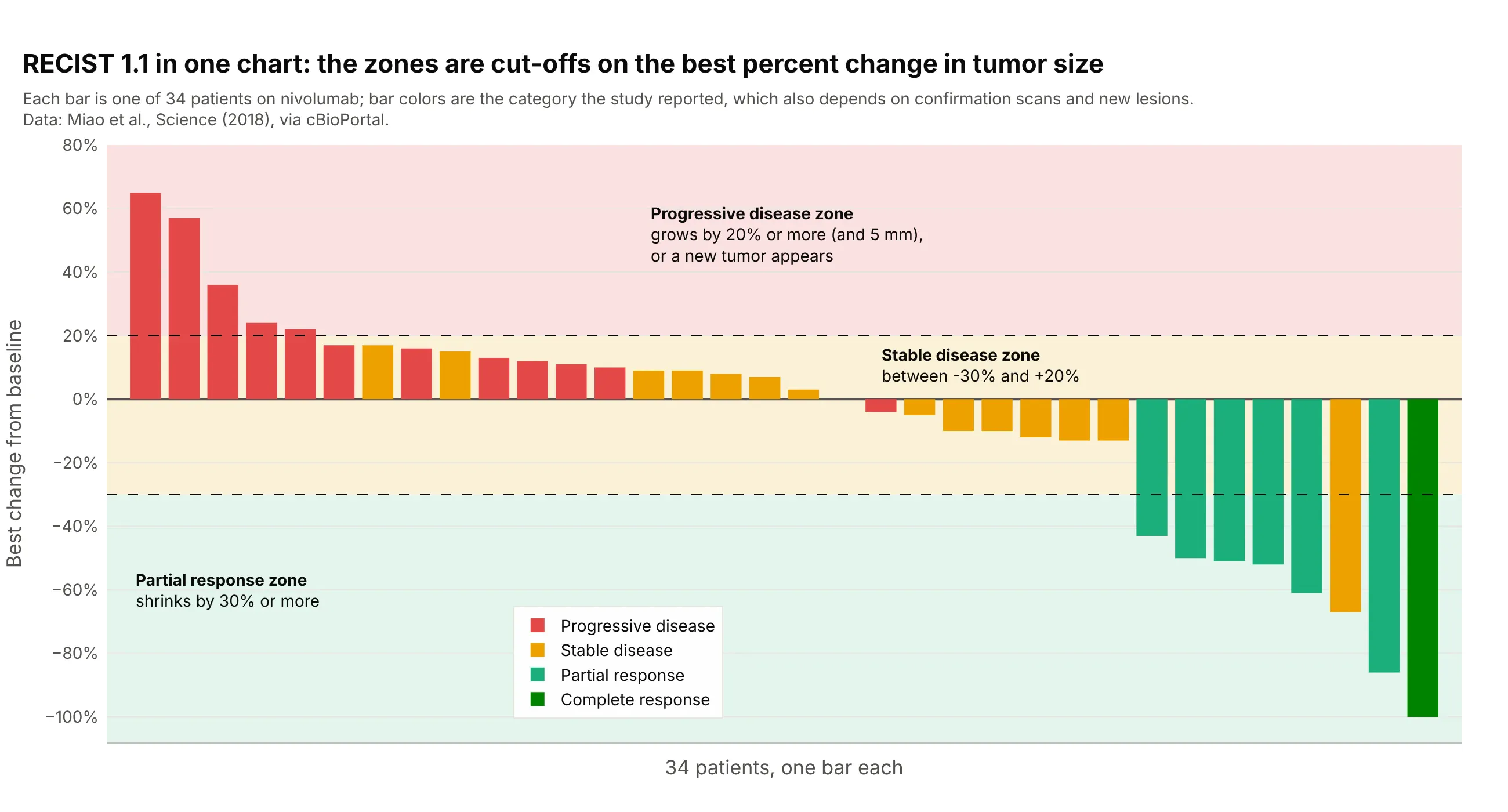
Data: Miao et al. (2018), Science, via cBioPortal.
Two bars sit in a different zone from the color they were reported with, a red bar at -4% and an orange one at -67%, because the category also depends on confirmation scans, on the non-target lesions that are followed but not measured, and on new tumors. Blood cancers, brain tumors, and PET-based trials use their own criteria (the Lugano classification, RANO for Response Assessment in Neuro-Oncology, and PERCIST for PET Response Criteria in Solid Tumors), but the waterfall plot is drawn the same way with the criteria's own cut-offs.
Alternatives to a tumor waterfall plot
Here's the same SUMMIT data drawn six ways. Some are better for the question, some worse, some just different:
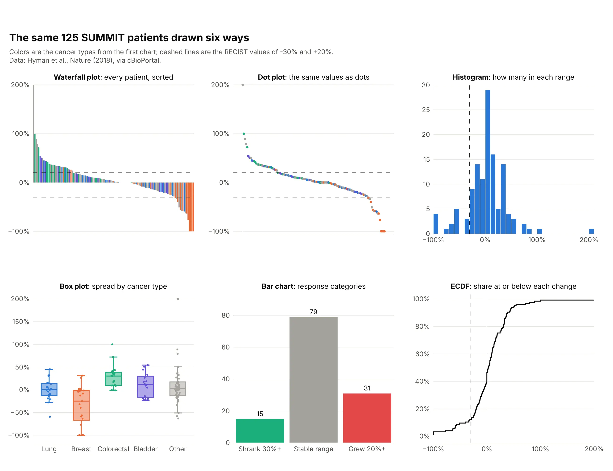
- Tumor waterfall plot (best for each patient's depth of response). It is the only one of the six where every patient is a mark you can point at, colored by a group, with the RECIST lines on it.
- Dot plot of the same values (works too). It carries the same information with less ink, which helps when there are hundreds of patients, but bars read more naturally as a response around a baseline of zero.
- Histogram (different). It shows the shape of the whole group, here a peak near zero with a tail of responders, and loses the patients.
- Box plot by cancer type (better for comparing groups). It makes the difference between breast cancer, with a median below -25%, and colorectal cancer visible at a glance, and it handles groups with many patients that a waterfall plot gets crowded by.
- Bar chart of response categories (worse for depth, standard for a headline). Fifteen, 79, and 31 patients is how a trial reports its response rate, and it drops how deep or how long.
- ECDF plot (works too). An empirical cumulative distribution function (ECDF) reads off the share of patients at or below any change and compares two arms of a trial on one axis.
- Swimmer plot (different). It shows how long each patient was treated instead of how deep the response was, and trial reports often show the two with the patients in the same order, as in example 4 below.
- Spider plot (different). It shows the path of each patient's tumor over time and needs scan-by-scan measurements, as in the xenograft example above.
- Forest plot (different). It summarizes response rates by subgroup with confidence intervals, which a waterfall plot can't.
For the second question a waterfall plot gets asked, how long a response lasts, here is the raw volume of the same melanoma tumors as the spider plot above:
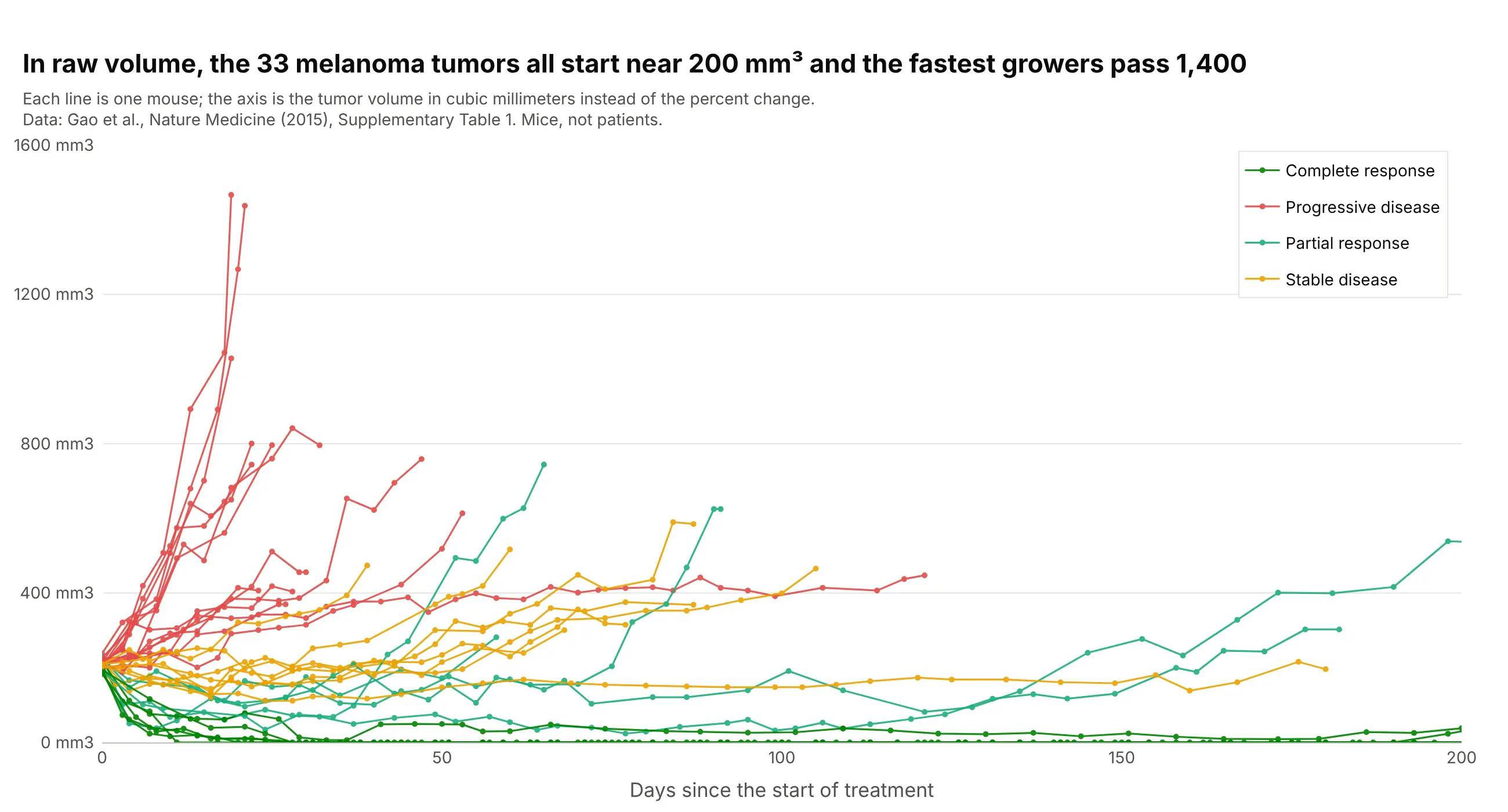
Data: Gao et al. (2015), Nature Medicine, Supplementary Table 1. Mice, not patients.
All 33 tumors start between 183 and 238 mm3, so for this dataset the percent change and the raw volume tell nearly the same story, and the spider plot is easier to compare across trials. When starting sizes differ a lot, the raw plot is the more honest one, which is the point of Mercier et al. (2019).
How to make a tumor waterfall plot
With AI
ChatGPT, Claude Code, GitHub Copilot, Cursor, and other AI tools are excellent at writing Plotly code. Name Plotly in the prompt, and say what the bars, the colors, and the dashed lines mean:
Make a plotly tumor waterfall plot from trial.csv (columns: patient, arm, best_response, best_change_pct).- One bar per patient with go.Bar, sorted from the largest best_change_pct on the left to the smallest on the right,colored by best_response (CR dark green, PR green, SD yellow, PD red).- Dashed horizontal lines at +20 (progressive disease) and -30 (partial response) with a label on each.- Leave out patients with an empty best_change_pct and print how many were left out.- Y axis titled "Best change from baseline" with % tick labels, no x tick labels, a legend that names every color.- Check: print how many patients are at -30 or lower.
With Plotly Studio
Plotly Studio is a product for creating data visualizations and Dash apps and for analyzing data with AI, available as a desktop app or embedded in Dash apps. Ask for a tumor waterfall plot the same way:
Show a waterfall plot of the best percent change in tumor size for each patient, sorted from growth to shrinkage and colored by dose level, with dashed lines at +20% and -30% and a dropdown to pick the trial arm.
Make a tumor waterfall plot in Python or JavaScript
This is the code AI tools write under the hood. Plotly's go.Waterfall draws the financial waterfall chart, so a tumor waterfall plot is a go.Bar trace with one bar per patient, sorted, plus add_hline for the dashed lines. This helper returns a go.Figure, and every example in this guide builds on the same idea:
import pandas as pdimport plotly.graph_objects as godef waterfall(df, value, color=None, colors=None, lines=(-30, 20)):"""A tumor waterfall plot in Plotly: one bar per patient, sorted from growth to shrinkage, RECIST lines."""df = df.dropna(subset=[value]).sort_values(value, ascending=False).reset_index(drop=True)fig = go.Figure()for key, g in df.groupby(color, sort=False) if color else [("", df)]:fig.add_trace(go.Bar(x=g.index, y=g[value], name=str(key), marker_color=(colors or {}).get(key),showlegend=bool(color)))for y in lines:fig.add_hline(y=y, line=dict(dash="dash", color="black", width=1))fig.update_layout(barmode="overlay", template="simple_white", xaxis_visible=False,yaxis=dict(title="Best change from baseline", ticksuffix="%"))return figdf = pd.read_csv("trap.csv") # patient, best_response, best_change_pct (Janjigian et al., Lancet Oncology 2020)fig = waterfall(df, "best_change_pct", color="best_response",colors={"CR": "#008300", "PR": "#1baf7a", "SD": "#eda100"})fig.show()
The x values are the positions after sorting, so the bars stay in order however many colors there are, and barmode="overlay" keeps each color's bars in their own place. A spider plot is one go.Scatter line per patient:
fig = go.Figure()for patient, g in scans.sort_values("day").groupby("patient"): # scans: patient, day, change_pctfig.add_trace(go.Scatter(x=g.day, y=g.change_pct, mode="lines+markers", name=patient, showlegend=False))fig.add_hline(y=0, line=dict(dash="dash", color="black", width=1))fig.update_layout(template="simple_white", xaxis_title="Days since start of treatment",yaxis=dict(title="Change from baseline", ticksuffix="%"))
In JavaScript, plotly.js draws the same waterfall plot with bar traces and two dashed lines as shapes:
<div id="chart"></div><script src="https://cdn.plot.ly/plotly-4.1.1.min.js"></script><script>// Best percent change for 35 patients (Janjigian et al., The Lancet Oncology 2020; cBioPortal egc_trap_msk_2020), sortedconst change = [-20, -25, -27.27, -31.6, -31.82, -33.3, -33.33, -42.42, -42.86, -43.48, -43.98, -44.6, -48.4, -48.9,-56.7, -58.62, -59.15, -62, -64.6, -64.84, -66.7, -68.2, -71.4, -71.43, -72.7, -72.7, -72.73, -76.92, -79.31, -80,-84.8, -100, -100, -100, -100];const x = change.map((_, i) => i);const bar = (name, color, keep) => ({type: "bar", name: name, marker: {color: color},x: x.filter(i => keep(change[i])), y: change.filter(keep)});Plotly.newPlot("chart", [bar("Shrank less than 30%", "#eda100", v => v > -30),bar("Shrank 30% or more", "#1baf7a", v => v <= -30)], {width: 900, height: 500, barmode: "overlay",xaxis: {visible: false},yaxis: {title: {text: "Best change from baseline (%)"}, range: [-105, 30]},shapes: [-30, 20].map(y => ({type: "line", xref: "paper", x0: 0, x1: 1, y0: y, y1: y, line: {dash: "dash", color: "black", width: 1}}))});</script>
Share it
Every Plotly chart has a Share chart button (the cloud icon in its toolbar) that uploads it to Plotly Cloud and gives you a link. Only you can see it until you change its visibility.
For a live app, put the chart in a Dash app and publish it with the Plotly Cloud CLI. Coding agents can run these commands for you:
pip install "dash[cloud]"plotly user loginplotly app publish
If your data has to stay in your own cloud or data center, publish to Dash Enterprise instead.
Dos and don'ts
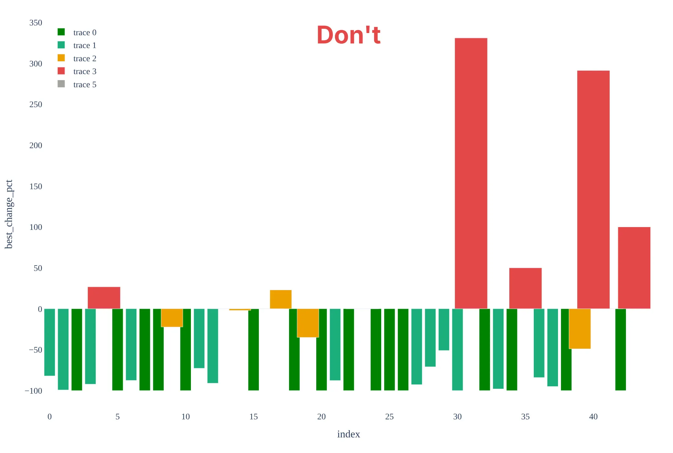
Most of the work in a waterfall plot is the order of the bars, the reference lines, and being honest about who is in it. Here are the 44 brain lymphoma patients both ways, with the same colors.
Don't order the bars by patient ID, plot the four patients who had no measurement as 0%, leave out the +20% and -30% lines, or keep the default legend ("trace 0"), raw column names, and a serif font:
Do sort the bars from growth to shrinkage, leave out the patients without a measurement and say how many there are, draw the RECIST lines, and name the colors and the axis in plain words:
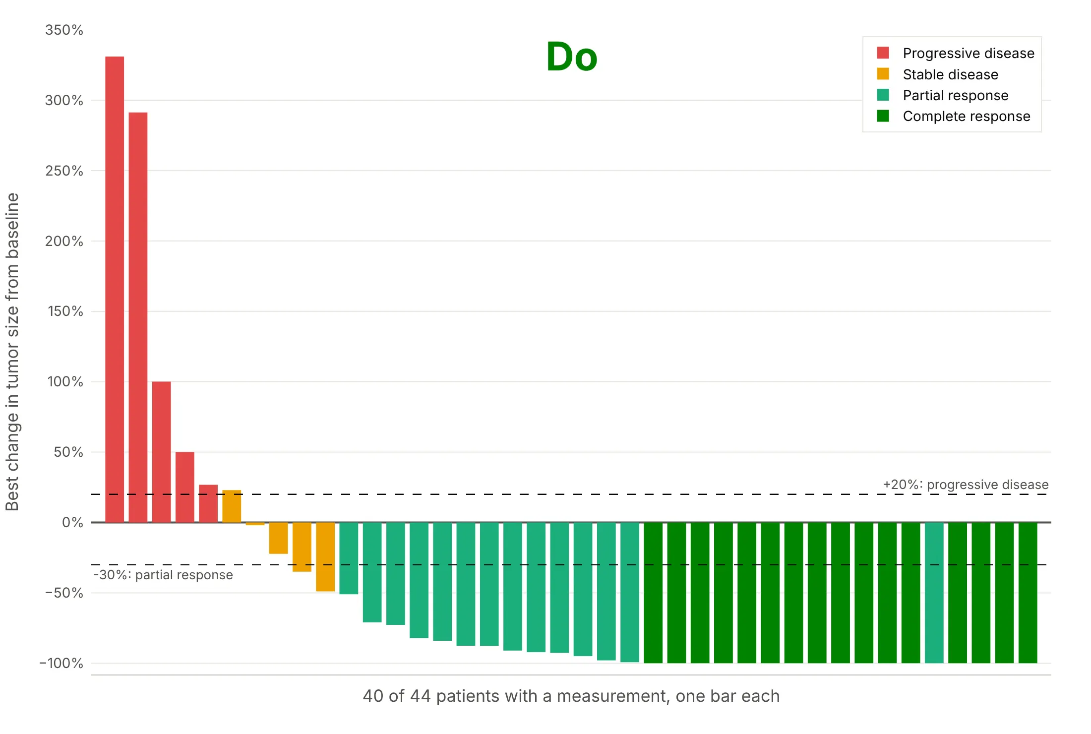
One light green bar, a partial response, sits at -100% among the dark green complete responses. A patient can be at -100% on the measured target tumors and still be reported as a partial response, because RECIST also follows non-target lesions, and a complete response needs all of them gone, and in a single-arm trial it needs a confirming scan at least four weeks later. The dataset gives only the percent change and the reported response, so it doesn't say which of these applies to that patient.
Checklist
Do
- Sort the bars by the best percent change, or group them first (by arm, dose, or cancer type) and sort inside each group.
- Say how many patients are shown out of how many were treated, and why the others are missing.
- Draw the +20% and -30% lines when the trial used RECIST 1.1, and name the criteria when it did not (PERCIST, RANO, Lugano).
- Color by something a reader can act on, such as best overall response, dose, arm, or a biomarker, and name every color.
- Cut the axis at a round number when one bar is far above the rest, and say so in the subtitle.
- Say when the data are from mice or another preclinical model, as in examples 5 and 6.
Don't
- Read the bar height as how long a response lasted: the waterfall plot has no time axis, so pair it with a swimmer plot or a spider plot.
- Compare two arms of a randomized trial with two waterfall plots alone, since a plot of the best change ignores follow-up time and doesn't test anything.
- Plot patients without a measurement as zero bars.
- Put patient names, initials, or dates of birth on the axis; use the study's anonymous ID or no labels.
- Use one bar per patient for hundreds of patients without thinning the bars or splitting the plot into panels.
More tumor waterfall plot examples
Six more plots built from real public data, each with its source, the technique that makes it work, and a prompt to rebuild it. Four are patient data from published trials, and the last two use tumors from a patient's cancer grown in mice, which is the only public source of scan-by-scan style tumor measurements that we found with a download link.
1. Color by dose: nivolumab in kidney cancer
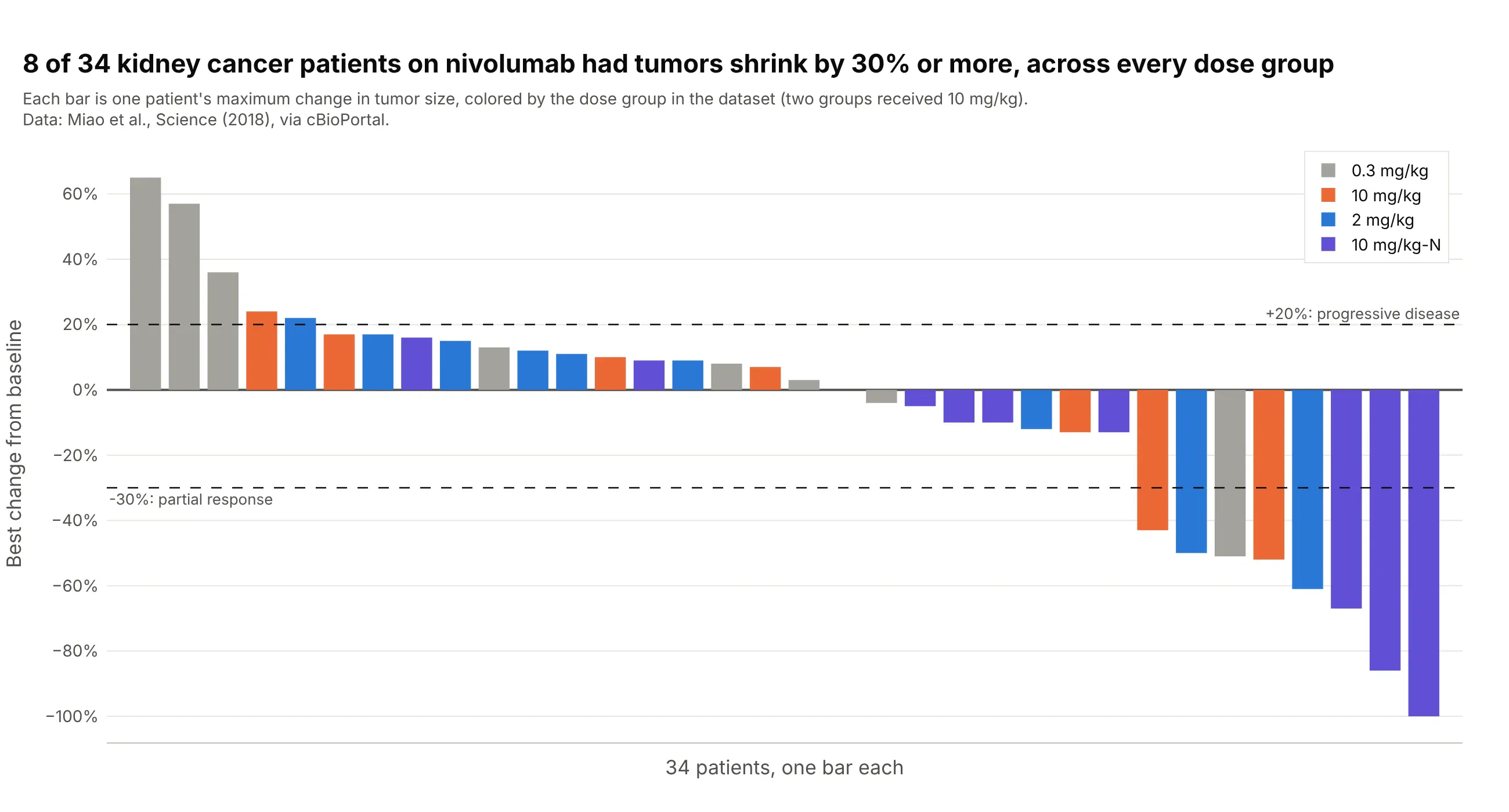
Eight of 34 patients with kidney cancer had tumors shrink by 30% or more on nivolumab, one of eight in the 0.3 mg/kg group, two of nine at 2 mg/kg, two of seven at 10 mg/kg, and three of ten in a second 10 mg/kg group, so the shrinkage does not belong to one dose. Data: Miao et al. (2018), Science, via cBioPortal.
Tip: when the groups have different sizes, say the count in each group in the legend or the subtitle.
Get the data from cBioPortal's study ccrcc_dfci_2019 (Miao et al., Science 2018, kidney cancer patients on nivolumab;patient attributes TREATMENT_GROUP, MAX_TUMOR_CHANGE and RECIST) and shape it into a table (columns: patient,dose_group, best_response, best_change_pct).Build a plotly tumor waterfall plot with one bar per patient, sorted from the largest to the smallest best_change_pct,colored by dose_group, with dashed lines at +20 and -30 and a legend that shows the number of patients in each group.
2. Color by biomarker: HER2 and HER3 mutations
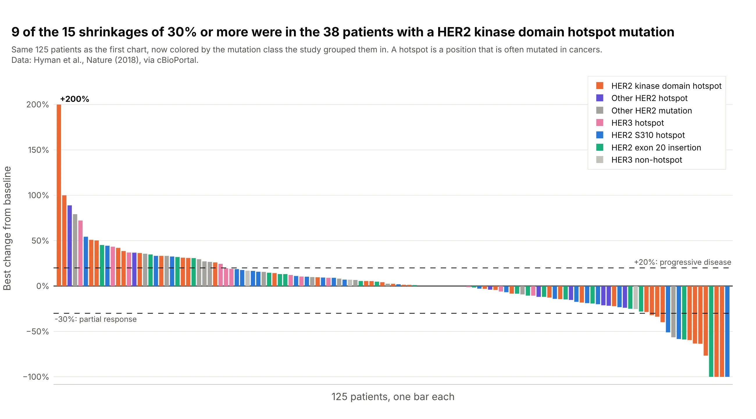
Nine of the 15 patients whose tumors shrank by 30% or more had a hotspot mutation in the kinase domain of HER2 (the part of the protein that sends growth signals), against none of the 15 patients with HER3 mutations. Coloring the same 125 bars by mutation class instead of cancer type shows which biomarker the response follows. Data: Hyman et al. (2018), Nature, via cBioPortal.
Tip: with more than five colors, use the same hue family for related classes and keep gray for the rest.
Get the data from cBioPortal's study summit_2018 (Hyman et al., Nature 2018, SUMMIT neratinib basket trial; sampleattributes TUMOR_CHANGE, WATERFALL_GROUP, GENE, CANCER_TYPE) and shape it into a table (columns: patient, cancer_type,mutation_class, best_change_pct), keeping patients with a TUMOR_CHANGE.Build a plotly tumor waterfall plot sorted by best_change_pct and colored by mutation_class, with dashed lines at +20and -30 and a title that says how many patients shrank by 30% or more and in which mutation class.
3. PET and CT on the same patients: cobimetinib
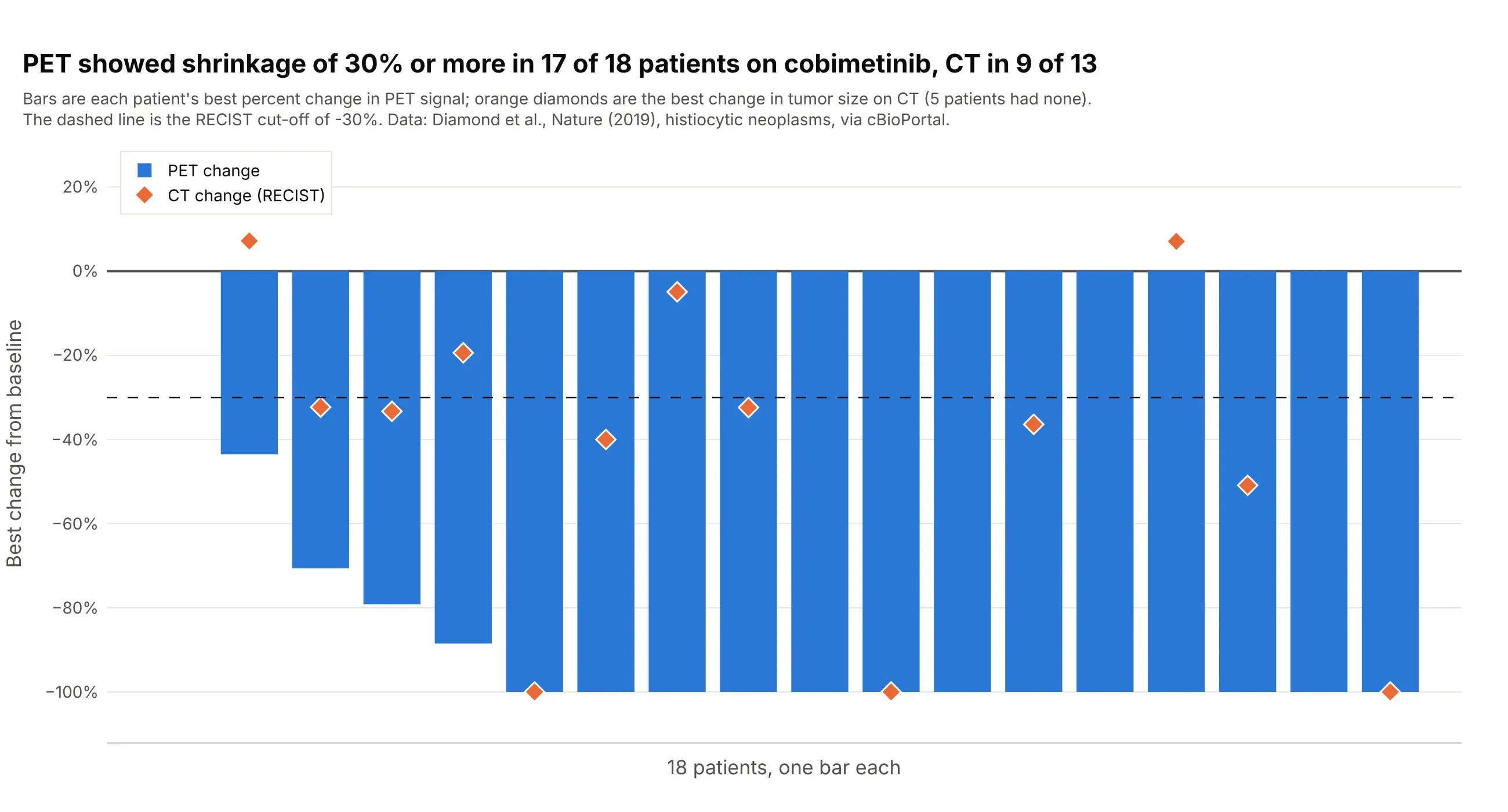
PET (positron emission tomography, a scan of how much tissue is metabolically active) showed shrinkage of 30% or more in 17 of 18 patients with histiocytic neoplasms, rare disorders of immune cells, treated with cobimetinib, a drug that blocks the MEK protein in a cell-growth signaling pathway, and 13 of them reached -100%, while CT showed it in 9 of the 13 patients who had a CT measurement. Putting both on one waterfall plot shows that two imaging methods can tell different stories for the same patient. Data: Diamond et al. (2019), Nature, trial NCT02649972, via cBioPortal.
Tip: draw the second measurement as markers on top of the bars instead of as a second bar, so the pairs stay aligned.
Get the data from cBioPortal's study histiocytosis_cobi_msk_2019 (Diamond et al., Nature 2019, cobimetinib inhistiocytic neoplasms; patient attributes PERCENT_CHANGE_BY_PET and PERCENT_CHANGE_BY_RECIST) and shape it into a table(columns: patient, pet_change_pct, recist_change_pct).Build a plotly waterfall plot with one blue bar per patient for pet_change_pct, sorted from the largest to the smallest,orange diamond markers for recist_change_pct on the same x positions, and a dashed line at -30.
4. Depth and duration together: a waterfall plot over a swimmer plot
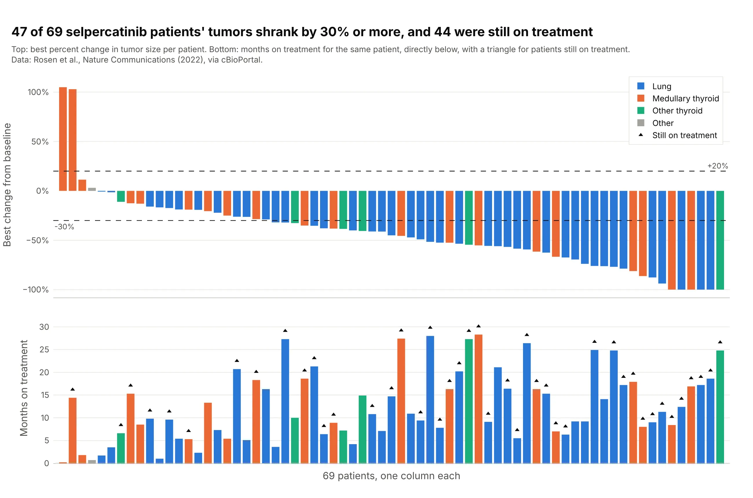
Forty-seven of 69 patients with RET-driven lung and thyroid cancers (cancers driven by a change in the RET gene) had tumors that shrank by 30% or more on selpercatinib, and 44 were still on treatment at data cutoff. Drawing months on treatment under each bar answers the question a waterfall plot can't, which is how long the shrinkage lasted, and it is the layout a swimmer plot pairs with. Data: Rosen et al. (2022), Nature Communications, via cBioPortal.
Tip: use make_subplots(shared_xaxes=True) and the same sorted index for both panels, so each column is one patient.
Get the data from cBioPortal's study mixed_selpercatinib_2020 (Rosen et al., Nature Communications 2022, selpercatinib inRET-driven cancers; patient attributes RECIST_RESPONSE, MONTHS_ON_TREATMENT, ONGOING_STATUS, ONCOTREE_PATIENT) and shapeit into a table (columns: patient, tumor, best_change_pct, months_on_treatment, ongoing).Build a plotly figure with make_subplots, two rows and shared x axes: a tumor waterfall plot on top (sorted, colored bytumor, dashed lines at +20 and -30) and bars of months_on_treatment below in the same order and colors, with a triangleabove the bars of patients with ongoing = 1.
5. Preclinical screens: 228 xenograft models and one drug
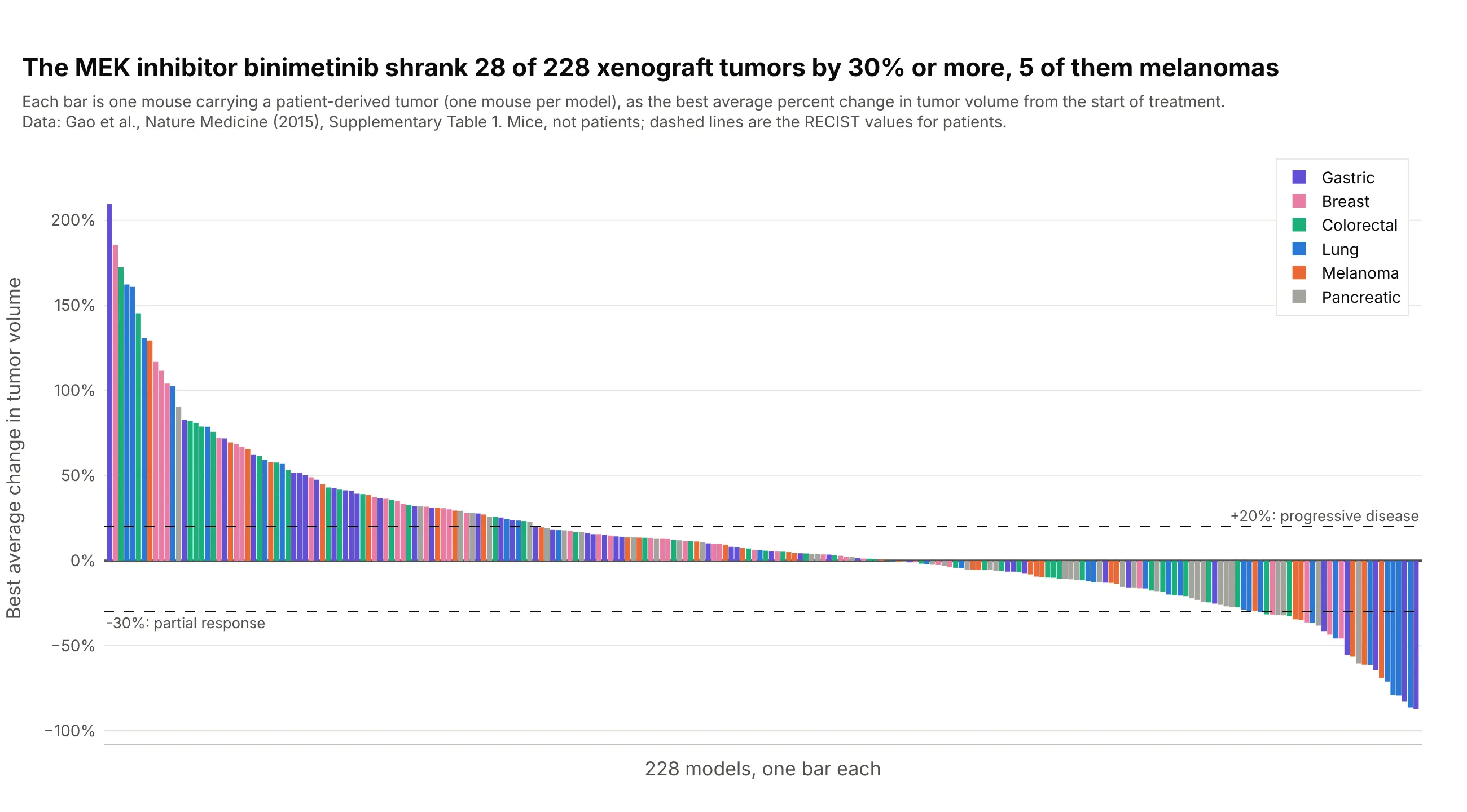
In a screen of about 1,000 models of patients' tumors grown in mice, with one mouse per model and treatment, binimetinib, a drug that blocks the MEK protein in a cell-growth signaling pathway, shrank 28 of 228 tumors by 30% or more, eight of them lung cancers and five melanomas, while 75 tumors grew by 20% or more. The paper's own waterfall plots use this design, so the chart reads like a trial. Data: Gao et al. (2015), Nature Medicine, Supplementary Table 1. Mice, not patients.
Tip: label preclinical data as preclinical in the subtitle, and say that the RECIST lines are borrowed from patients.
Get the data from the Excel file Supplementary Table 1 of Gao et al., Nature Medicine 2015 (doi 10.1038/nm.3954), sheet"PCT curve metrics" (columns Model, Treatment, BestAvgResponse) plus the tumor type of each model from the sheet "PCT rawdata", and shape it into a table (columns: model, tumor, treatment, best_avg_pct) for the treatment binimetinib.Build a plotly tumor waterfall plot with one bar per model, sorted from the largest to the smallest best_avg_pct andcolored by tumor type, with dashed lines at +20 and -30, and a subtitle that says the animals are mice.
6. Two treatments in the same models
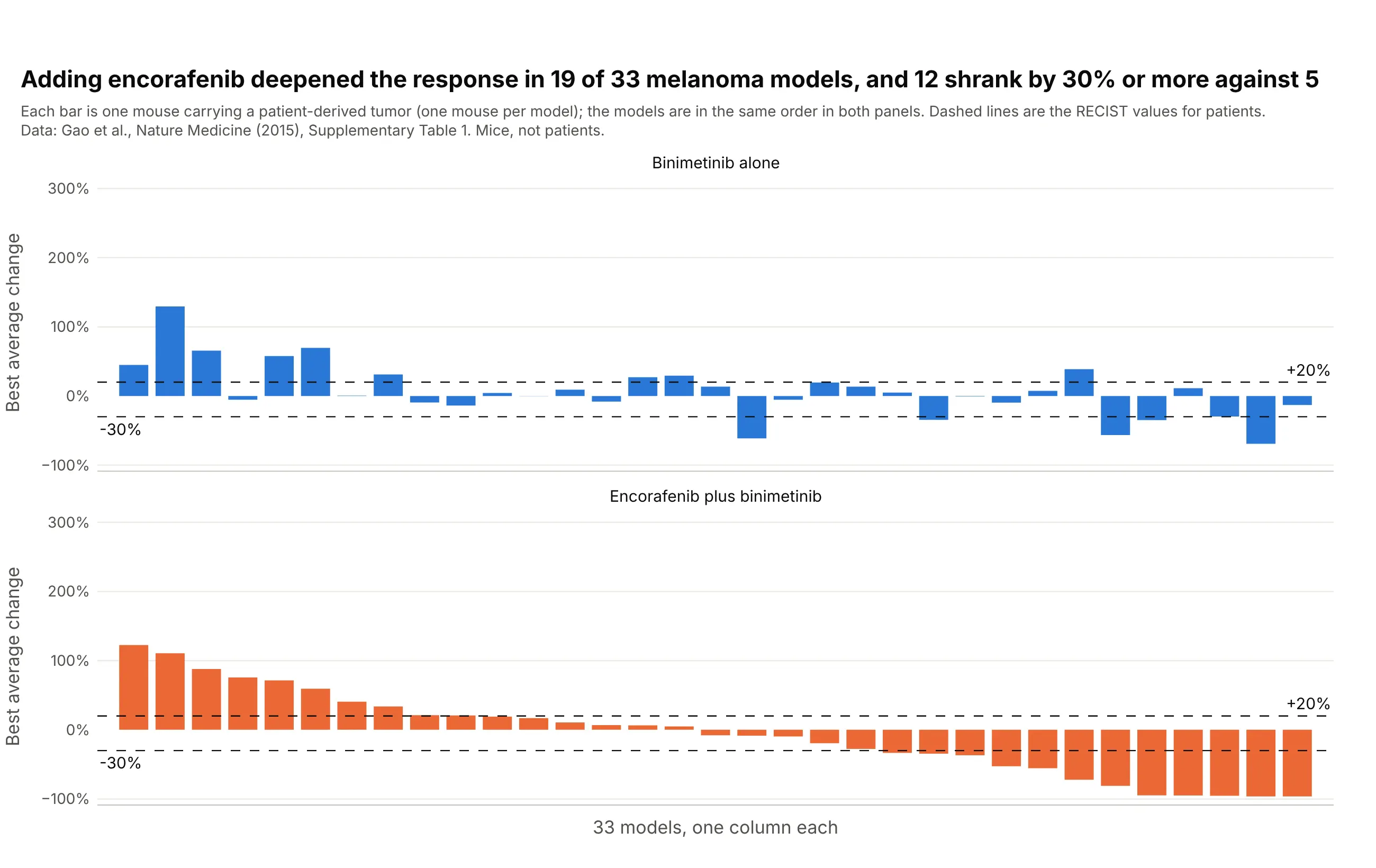
Adding encorafenib to binimetinib gave a deeper best average response in 19 of 33 melanoma models, and 12 shrank by 30% or more against five on binimetinib alone. Keeping the models in the same order in both panels, sorted by the combination, shows the effect of the second drug on each model. Data: Gao et al. (2015), Nature Medicine, Supplementary Table 1. Mice, not patients.
Tip: sort both panels by one treatment, so the other panel shows how far each bar moved.
Get the data from the Excel file Supplementary Table 1 of Gao et al., Nature Medicine 2015 (doi 10.1038/nm.3954), sheet"PCT curve metrics" (columns Model, Treatment, BestAvgResponse) and the tumor type of each model from the sheet "PCT rawdata", and shape it into a table (columns: model, binimetinib_pct, combination_pct) for the melanoma (CM) models thathave both treatments "binimetinib" and "encorafenib + binimetinib".Build a plotly figure with make_subplots, two rows and shared x axes, one waterfall plot per treatment with the models inthe same order sorted by combination_pct, dashed lines at +20 and -30, and a title with how many models improved.
FAQ
Options to customize
A tumor waterfall plot in Plotly is a bar trace plus reference lines, so these are the options that matter most. The full lists are in the bar trace reference and the layout reference.
- go.Bar(x=..., y=...): one bar per patient; x is the sorted position and y the best percent change.
- marker.color: one color for all bars, or a list with a color per bar, for example by response category; see bar chart styling.
- barmode="overlay": keeps bars from different color traces in their own positions when you draw one trace per group.
- bargap and width: the space between bars; 0.1 to 0.2 for a few dozen patients and 0 for hundreds.
- fig.add_hline(y=-30) and y=20: the RECIST lines; use line_dash="dash" and annotation_text to label them.
- yaxis.ticksuffix="%" and yaxis.range: percent tick labels, and a fixed range such as -105 to 110 so the floor at -100% is visible.
- xaxis.visible=False or showticklabels=False: hide the position numbers, or put patient IDs there with tickvals and ticktext when the IDs are anonymous.
- go.Scatter(mode="markers") on the same x positions: a second measurement (CT over PET), a star for a complete response, or a triangle for an ongoing patient; see the marker symbols.
- hovertemplate with customdata: patient ID, dose, and best response on hover.
- make_subplots(rows=2, shared_xaxes=True): a waterfall plot above a swimmer-style bar chart, or one panel per arm; see subplots.
- go.Scatter(mode="lines+markers") with one trace per patient: a spider plot, with line.color by response and add_hline(y=0) for the baseline.