Histograms - A Complete Guide

TL;DR

• A histogram splits a range of numbers into bins and draws one bar per bin, as tall as the number of values in it, so it shows where values pile up, how far they spread and what the tails look like.
• The bin width changes what you see. Rules like Freedman-Diaconis give a starting point, but try a few widths and line the bin edges up with how the data was rounded.
• Use a box plot for many groups and an ECDF for exact percentiles, and a bar chart (not a histogram) for categories.
• Any coding agent can make one with Plotly in a minute. In Python it's px.histogram(df, x="value").

What is a histogram?

Histograms look like this:

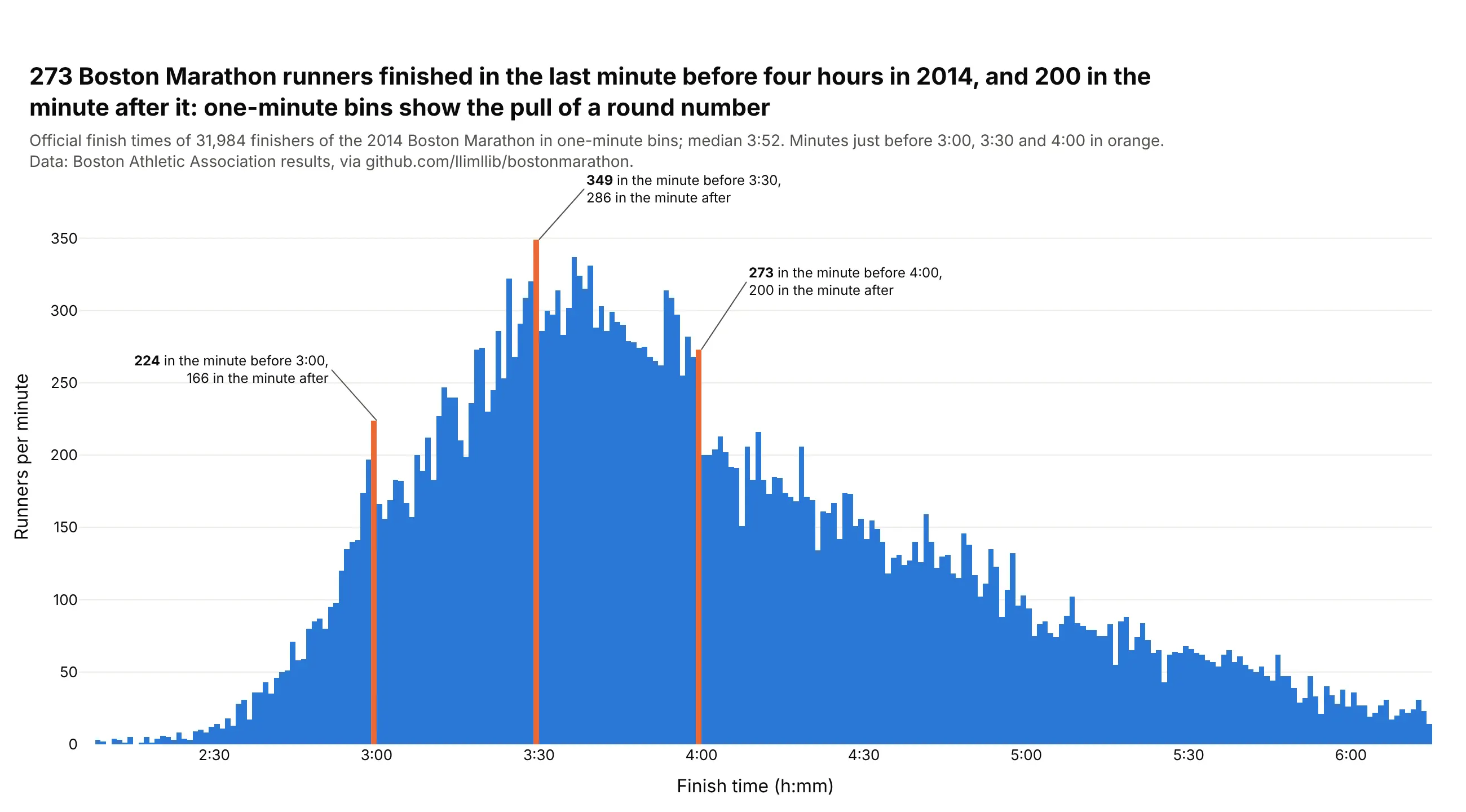
Data: Boston Athletic Association 2014 results via github.com/llimllib/bostonmarathon.

How do you read a histogram? In the example above, notice these things:

• Each bar covers one minute of finish time in the 2014 Boston Marathon, and its height is the number of runners who crossed the line in that minute.
• The bars touch and stand on a shared zero line, so the overall shape reads at once, with a peak around three and a half hours and a long tail of slower runners stretching to the right.
• The long right tail pulls the middle of the data to the right of the tallest bars, so the median finish time of 3:52 is later than the peak suggests.
• The orange bars mark the last minute before the round goal times, and each one is taller than the bar right after it because runners close to a goal push to get under it.
• The bin width decides what you can see. These spikes only show up because the bins are one minute wide, and wider bins would smooth them away, so try more than one width before you decide a histogram has no detail.

It's often used for charts like these:

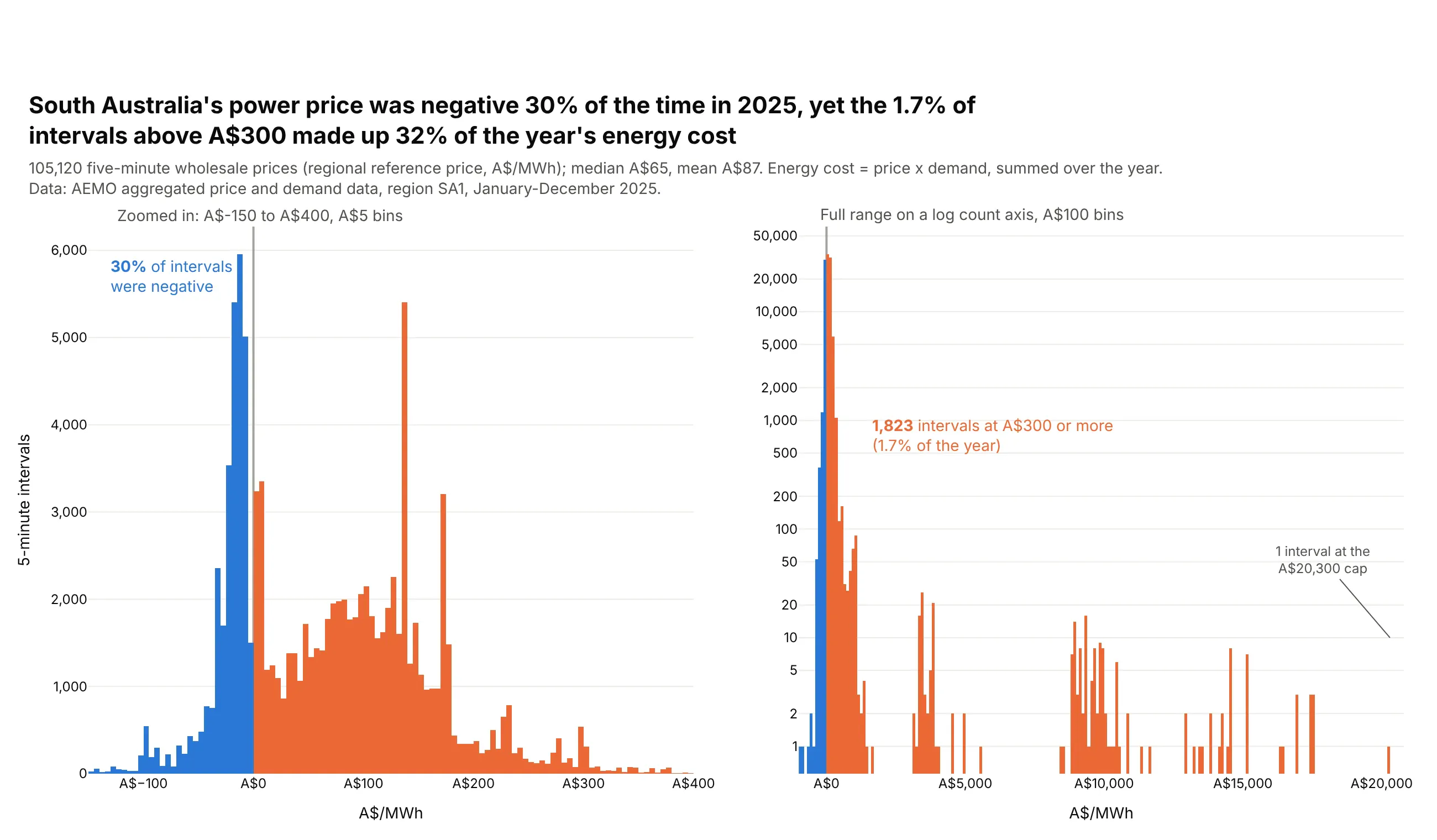
Prices. South Australia's wholesale power price was negative in 30% of 2025's 5-minute intervals, and one interval hit the A$20,300 cap, which a log count axis on the right panel keeps visible. Data: AEMO aggregated price and demand data, SA1, 2025.

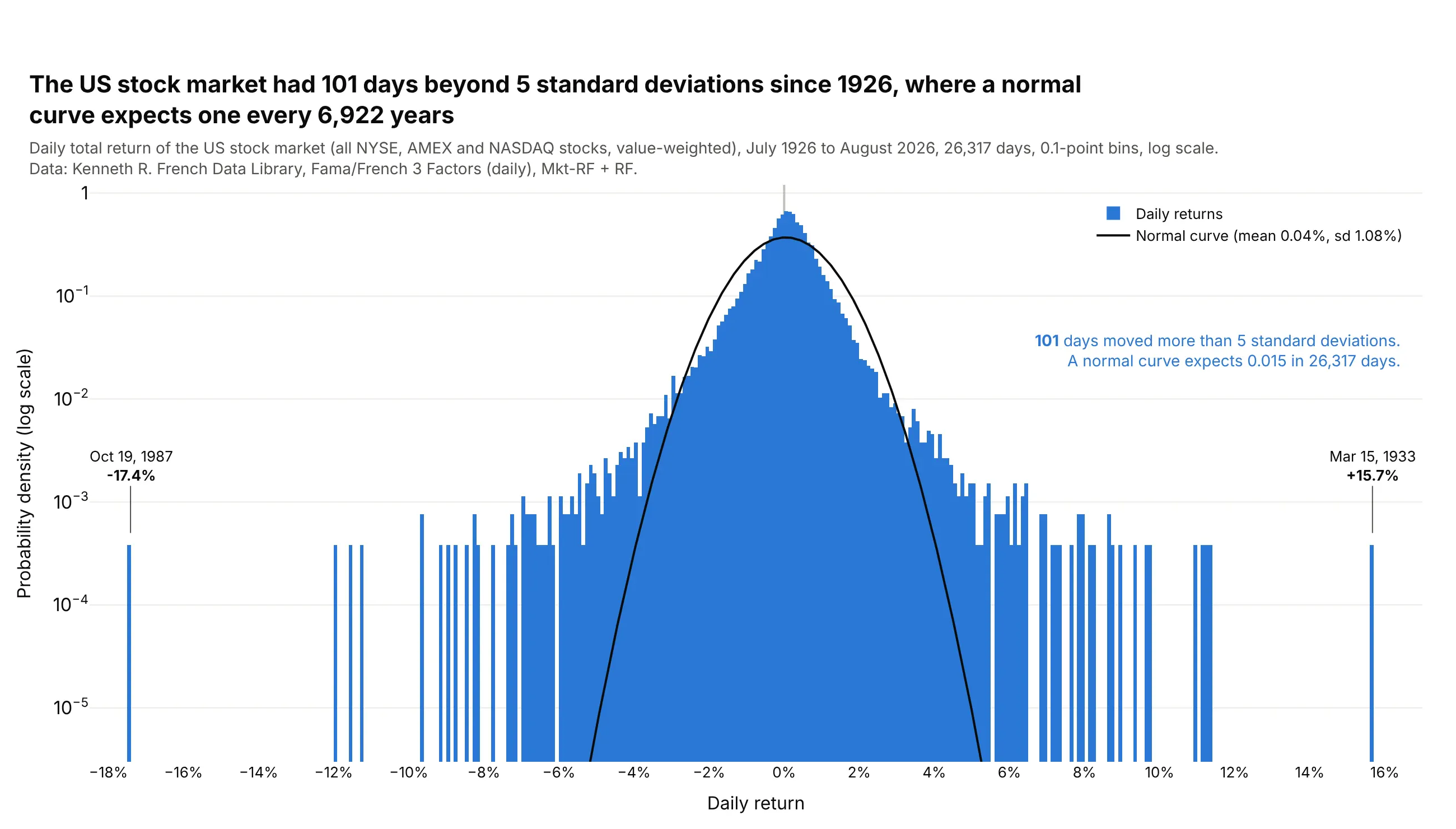
Returns against a model. Since 1926 the US stock market had 101 days that moved more than 5 standard deviations, where a normal curve with the same mean and spread expects 0.015 such days. Data: Kenneth R. French Data Library, Fama/French 3 Factors (daily).

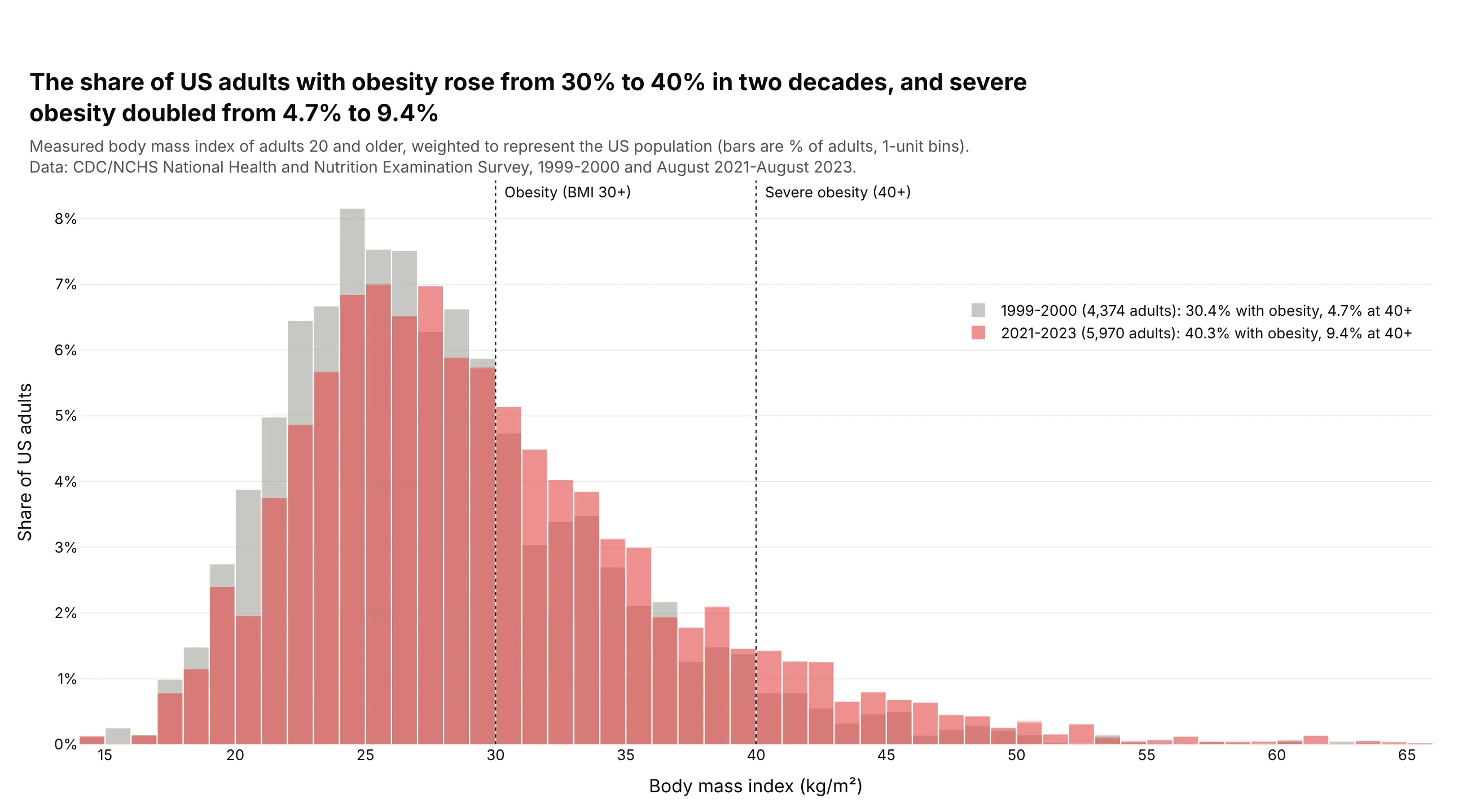
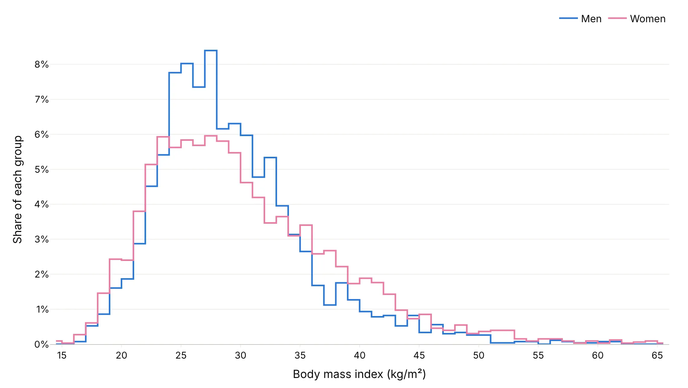
Two groups or two years. The share of US adults with a BMI of 30 or more rose from 30.4% in 1999-2000 to 40.3% in 2021-2023, and the whole distribution moved right. Data: CDC/NCHS NHANES, 1999-2000 and August 2021-August 2023.

A short history

Karl Pearson introduced the word "histogram" in his 1891 lectures and used it in print in "Skew Variation in Homogeneous Material" (1895). How many bins to use came later: Herbert Sturges proposed log2(n) + 1 bins in "The Choice of a Class Interval" (1926), David Scott derived a width from the standard deviation in "On optimal and data-based histograms" (1979), and David Freedman and Persi Diaconis used the interquartile range instead, so outliers don't stretch the bins, in "On the histogram as a density estimator" (1981).

Alternatives to a histogram

Here's the same 5,305 summer days in Phoenix (daily highs in June-August of 1940-1969 and 1996-2025) drawn six ways. Some are better for the question, some worse, some just different:

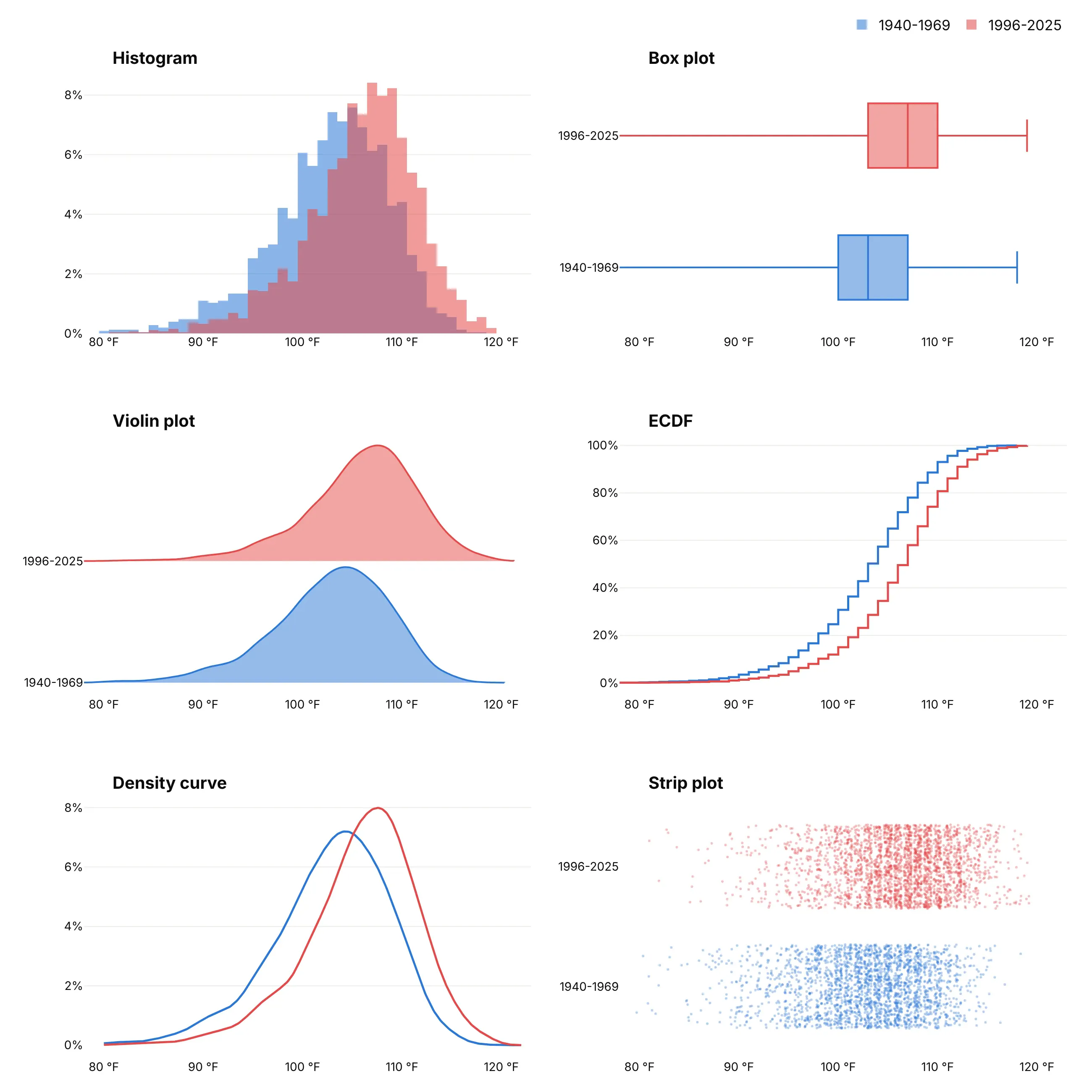
• Box plot (better for many groups). It reduces each group to a median, quartiles and whiskers, here 103 °F against 107 °F, so dozens of groups fit side by side, but it hides the shape of the distribution. See our box plot guide.
• Violin plot (different). A smoothed shape per group, mirrored or one-sided, which fits more groups than overlaid histograms but depends on the smoothing bandwidth. See our violin plot guide.
• ECDF (better for exact percentiles). The share of days at or below each temperature, with no bins to choose, so you can read off any percentile, but most readers need a moment to learn it.
• Density curve (works too). A kernel density estimate is a histogram with the steps smoothed away, which reads well for two or three groups. Like the violin, it depends on its bandwidth and can draw values that don't exist past the ends of the data.
• Strip plot (better for small samples, worse here). Every value as a dot shows exactly what you have when there are a few dozen values, but at 5,305 days the dots blur into two bands.

For many groups at once, a ridgeline plot stacks one density curve per group.

How to make a histogram

With AI

ChatGPT, Claude Code, GitHub Copilot, Cursor and other AI tools are excellent at writing Plotly code. Name Plotly in the prompt, spell out the bins, the normalization and the comparison, and list the checks you want:

With Plotly Studio

Plotly Studio is a desktop app where you point an AI at a dataset and it builds charts and a Dash app around your questions. Ask for a histogram and say what the bins and the comparison should be:

Show a histogram of 5-minute power prices with bins of A$5 from -150 to 400, negative prices in blue and the rest in orange, and a second panel with the full range on a log count axis. Add a dropdown to pick the region and a slider for the bin width.

Make a histogram in Python or JavaScript

This is the code AI tools write under the hood. In Python, Plotly Express makes one in one line, and xbins sets the bin edges exactly:

In JavaScript, plotly.js takes the raw values and bins them in the browser:

For millions of values, bin first with numpy.histogram, pandas or SQL and draw the counts with go.Bar, or pass them to go.Histogram as y with histfunc="sum" (see the FAQ for timings).

Share it

Every Plotly chart has a Share chart button (the cloud icon in its toolbar) that uploads it to Plotly Cloud and gives you a link. Only you can see it until you change its visibility.

For a live app, put the chart in a Dash app and publish it with the Plotly Cloud CLI. Coding agents can run these commands for you:

If your data has to stay in your own cloud or data center, publish to Dash Enterprise instead.

Dos and don'ts

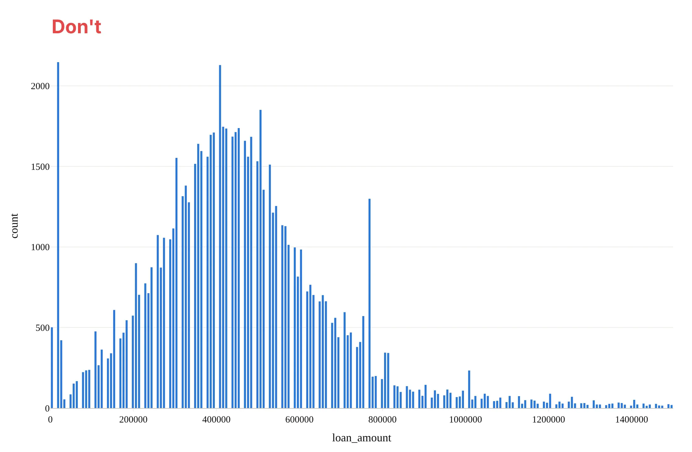
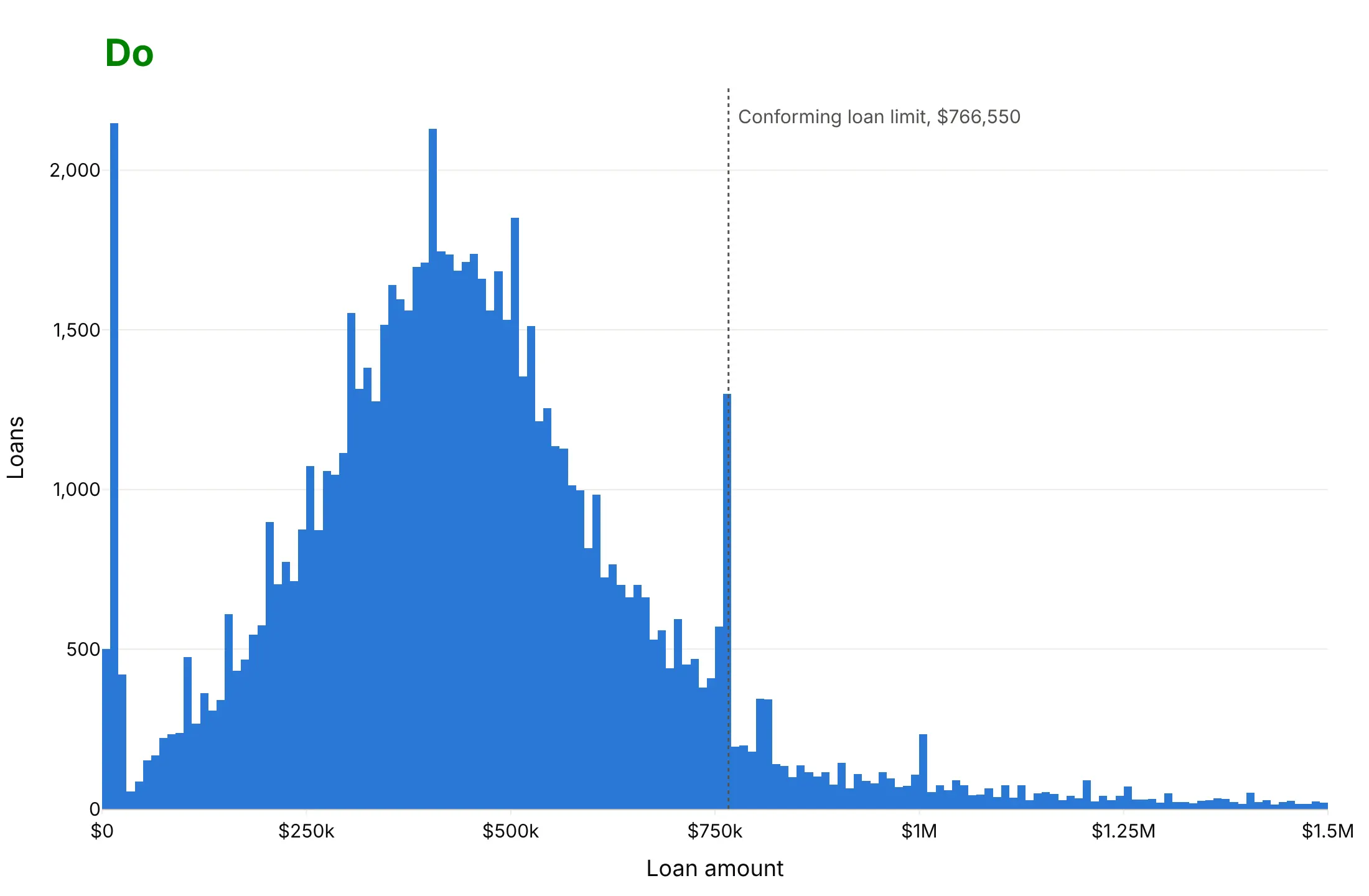
For a histogram you publish, most of the work is choosing the bins and labeling the axes. Here are 79,809 Colorado home purchase loans from 2024 both ways, in the same color. HMDA rounds every loan amount to the middle of a $10,000 interval, and 1,219 loans above $1.5 million are off the right edge of both charts.

Don't use bins that fight the data's rounding, leave gaps between bars, print raw numbers like 1000000 or column names as axis titles, or leave out the reference value the chart is about. Here $7,500 bins split the $10,000 steps unevenly, so every fourth bin is empty and the chart looks like a comb:

Do use $10,000 bins starting at $0, so each bar holds exactly one of HMDA's rounding steps, let the bars touch, format the axis in dollars and mark the conforming loan limit. The spike just under the $766,550 limit, 1,299 loans, is now the clear story:

Try more than one bin width

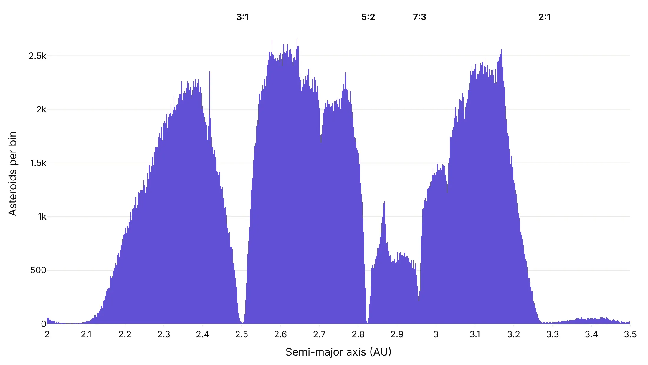
The bin width decides what you see, so try a few before you describe the shape. These are the semi-major axes of 857,193 asteroids from NASA/JPL's Small-Body Database.

Too wide. Sturges' rule gives 21 bins of 0.071 AU, which shows a lumpy plateau and hides the gaps that Jupiter's gravity clears in the belt.

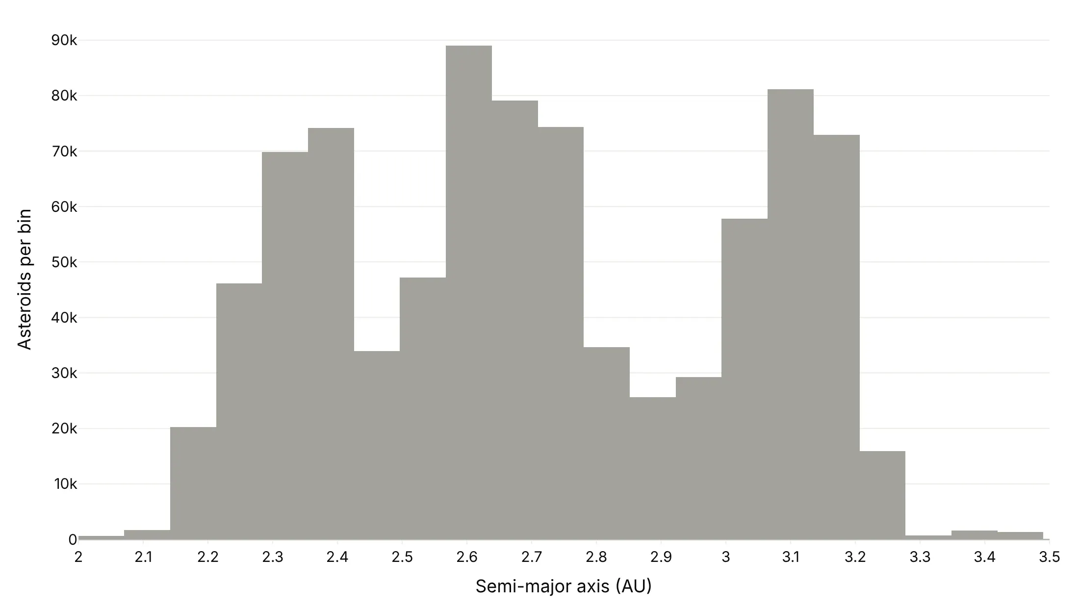
Narrow enough. At 0.002 AU, the Kirkwood gaps at the 3:1, 5:2, 7:3 and 2:1 resonances with Jupiter drop to almost nothing. The Freedman-Diaconis rule (2 x IQR / n^(1/3)) gives 0.012 AU here, which already shows the dips and is a good default.

Comparing two groups

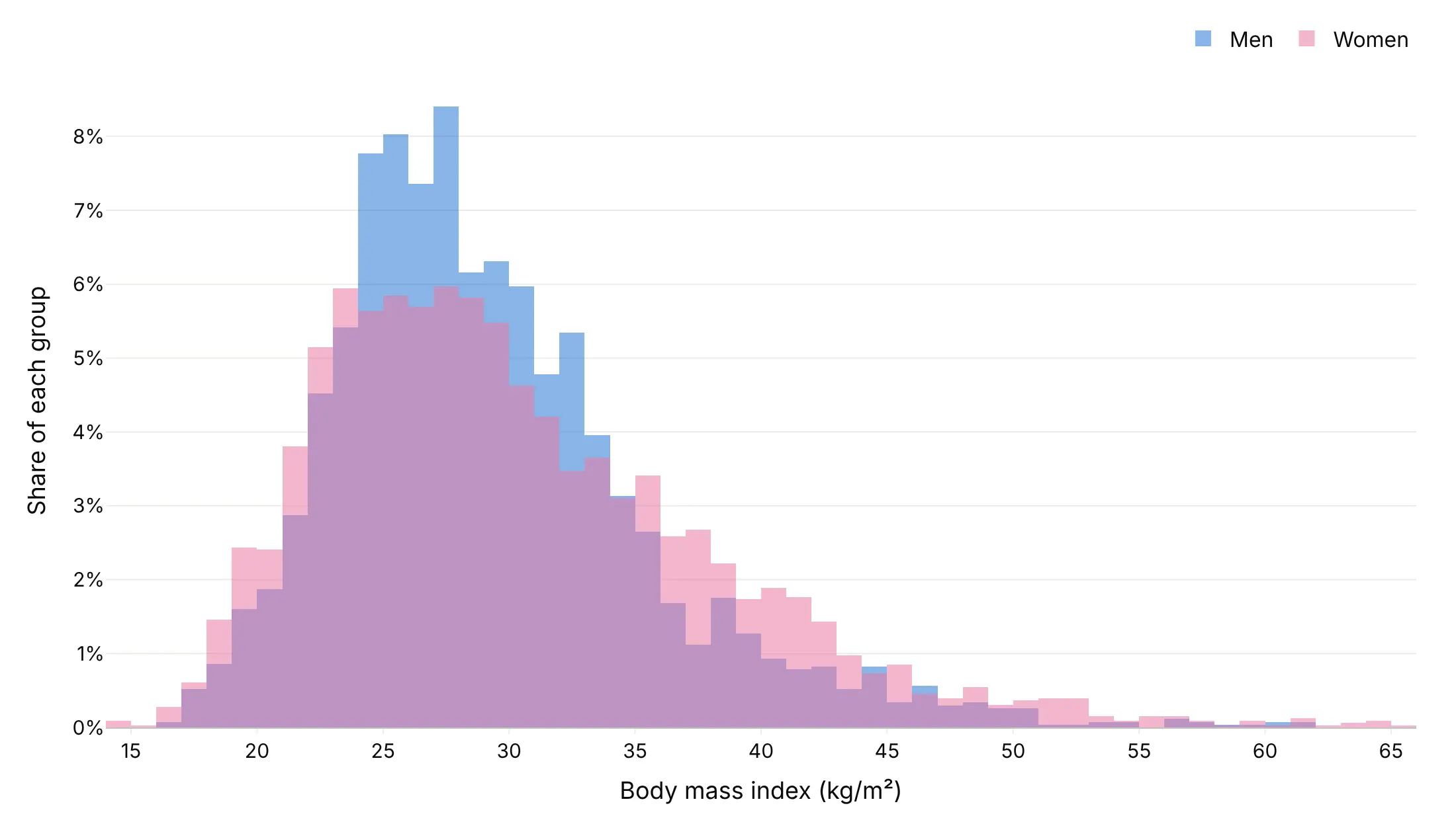
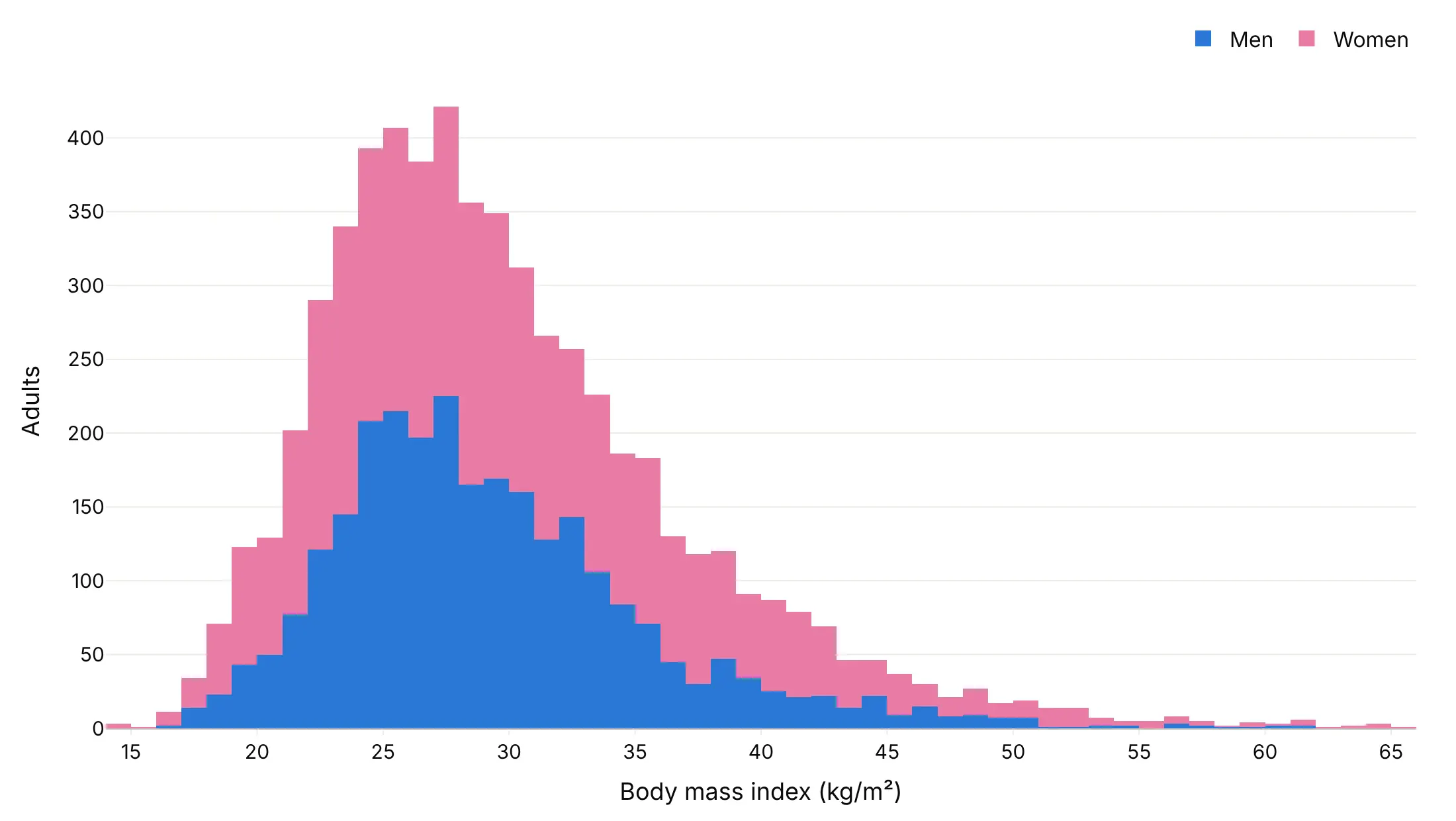
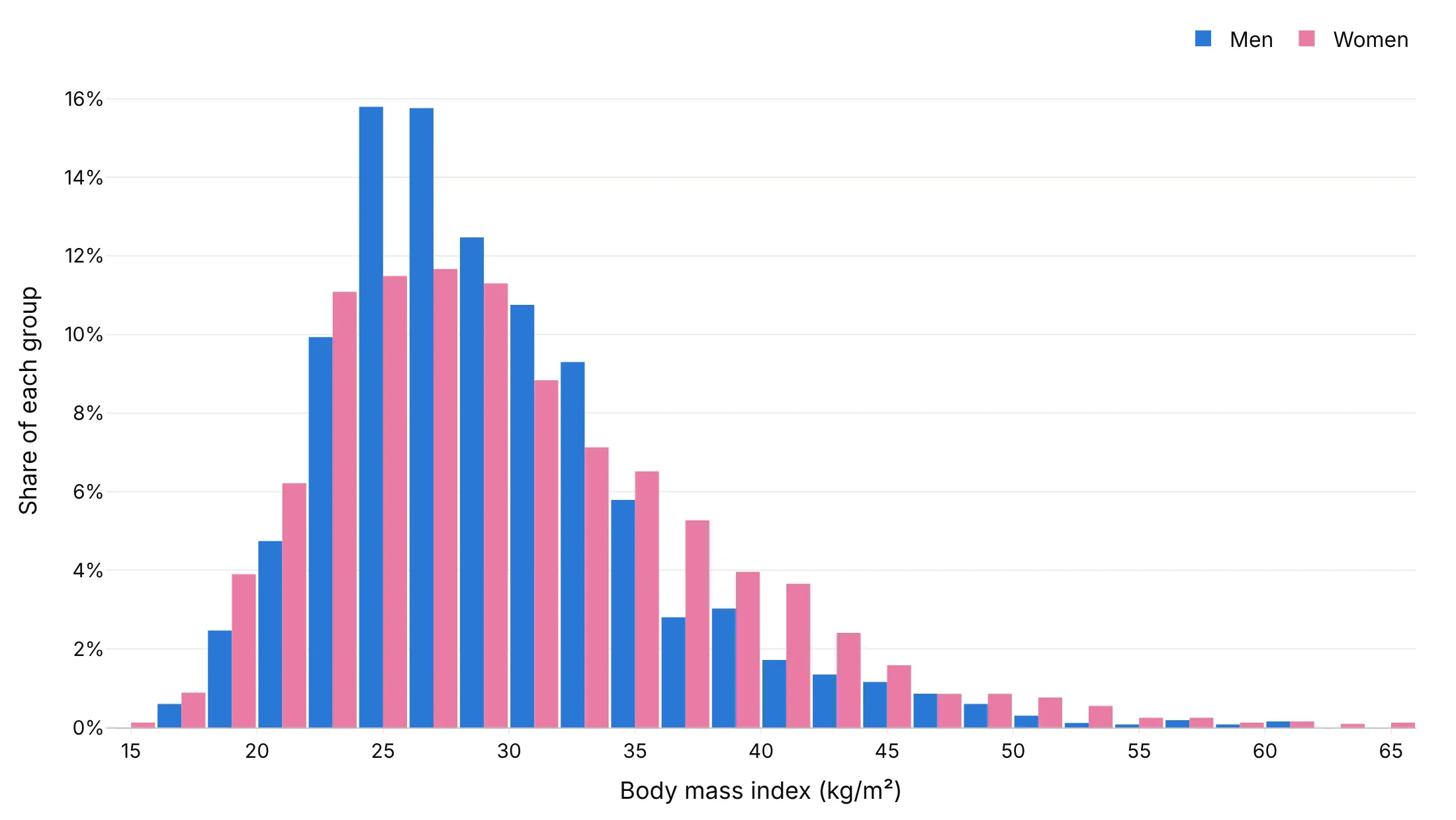
The layout matters as much as the bins when you compare groups. Here are the BMIs of 2,680 US men and 3,290 women aged 20 and older (NHANES, August 2021-August 2023) four ways.

Overlaid with barmode="overlay" and some opacity. The shapes compare directly, and it works for two groups, but the overlap mixes the colors.

Stacked (avoid for shape). The top shows the total, but only the bottom group sits on a flat baseline, so women's shape is hard to read.

Side by side with barmode="group". Every bar is readable, but it needs bins twice as wide, here 2 BMI units.

Step outlines. Counts from numpy.histogram drawn as lines with line_shape="hvh" overlap cleanly, and they're our choice for two or three groups.

Checklist

Do

• Set the bins yourself with xbins=dict(start=..., size=...) once you know the data, so the chart doesn't change when the data does.
• Align bins with how the data was rounded: whole degrees, whole minutes, $10,000 intervals.
• Cap the axis at a sensible range and say how many values are off it.
• Use histnorm="percent" when groups differ in size.
• Use a log axis for heavy tails: log counts for rare extremes, log-spaced bins for sizes across orders of magnitude.
• Mark reference values (a limit, a threshold, the median) with add_vline.

Don't

• Overlay more than two or three groups; use small multiples or a ridgeline plot.
• Stack groups when the question is about each group's shape.
• Add gaps between bars with bargap, which makes it look like a bar chart of categories.
• Describe the shape after trying only one bin width.

Options to customize

These are the go.Histogram (and px.histogram) options that matter most. The full list is in the Plotly histogram documentation.

1. x, y: the values to bin (x for vertical bars, y for horizontal); with both, y is aggregated by histfunc.
2. nbinsx, nbinsy: a maximum number of bins, for quick exploring; Plotly picks a round width.
3. xbins (start, end, size): exact bin edges and width, for publishing, rounded data and matching bins across traces.
4. histnorm: "" (counts), "percent", "probability", "density" or "probability density", for groups of different sizes or bins of different widths.
5. histfunc: "count", "sum", "avg", "min" or "max" of y per bin, for summing capacity or survey weights and for pre-binned counts.
6. cumulative (enabled, direction, currentbin): a running total across bins, for "what share is below x?" questions.
7. barmode (layout): "overlay", "stack" or "group", for comparing groups.
8. opacity: transparency of the bars, for overlaid groups.
9. bargap, bargroupgap (layout): space between bars; keep bargap at 0 or close to it.
10. orientation: "v" or "h", for horizontal and back-to-back histograms.
11. bingroup: makes traces share the same bins.
12. marginal (px only): a "histogram", "box", "violin" or "rug" beside the main chart.
13. go.Histogram2d (xbins, ybins, z, colorscale): 2D histograms of two variables and pre-binned grids.
14. hovertemplate: the hover text, for example the bin range and its share.

More histogram examples

Eleven more histograms built from real public data, each with its source, the technique that makes it work and a prompt to rebuild it.

1. When today's US power plants were built

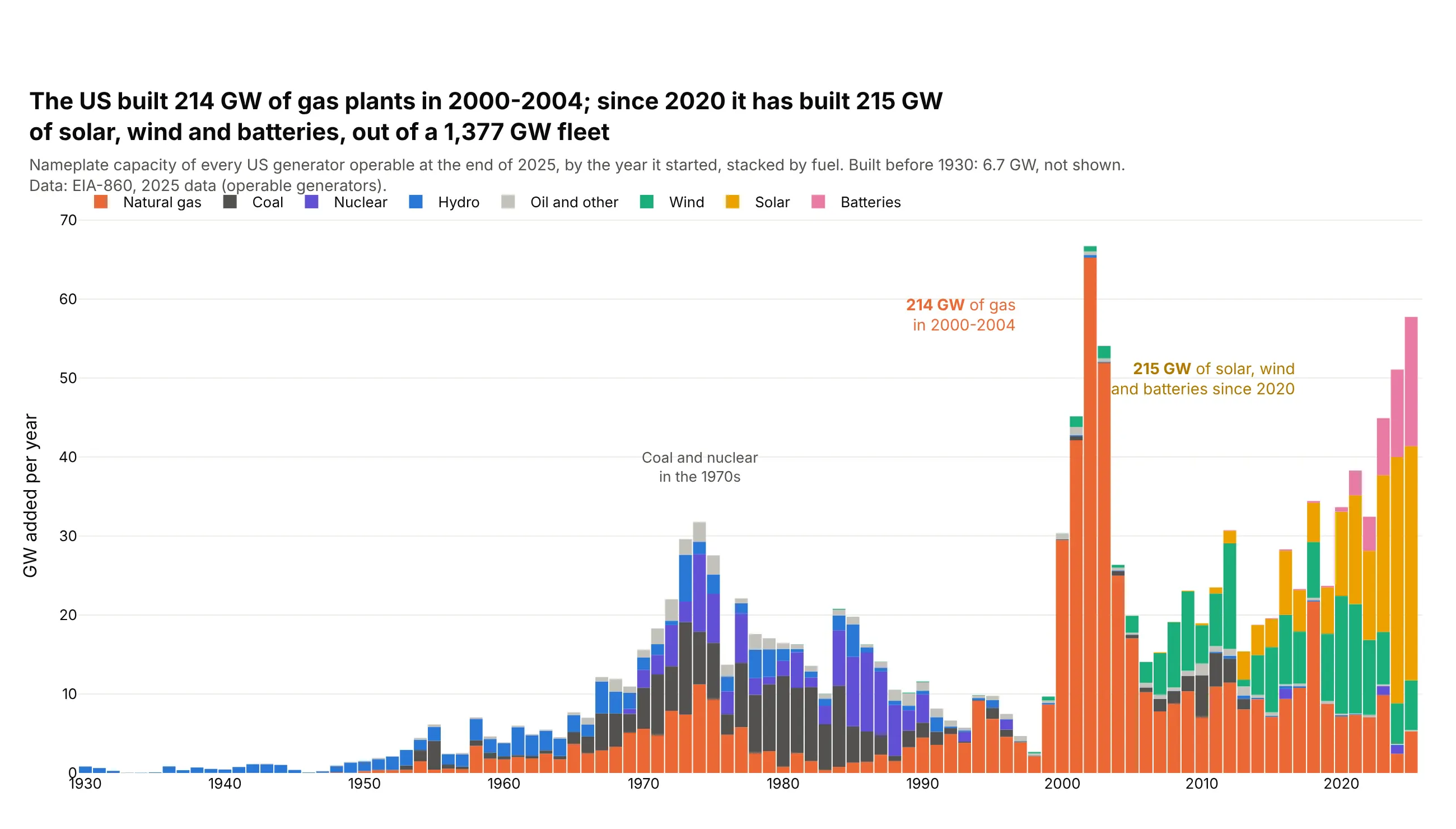
The US built 214 GW of gas plants in 2000-2004, 16% of today's 1,377 GW fleet. Since 2020 it has added 215 GW of solar, wind and batteries, and 2025 alone added 58 GW. Data: EIA-860, 2025 data.

Tip: histfunc="sum" with y set to capacity turns a count of generators into GW built per year.

2. Wind turbine rotors, decade by decade

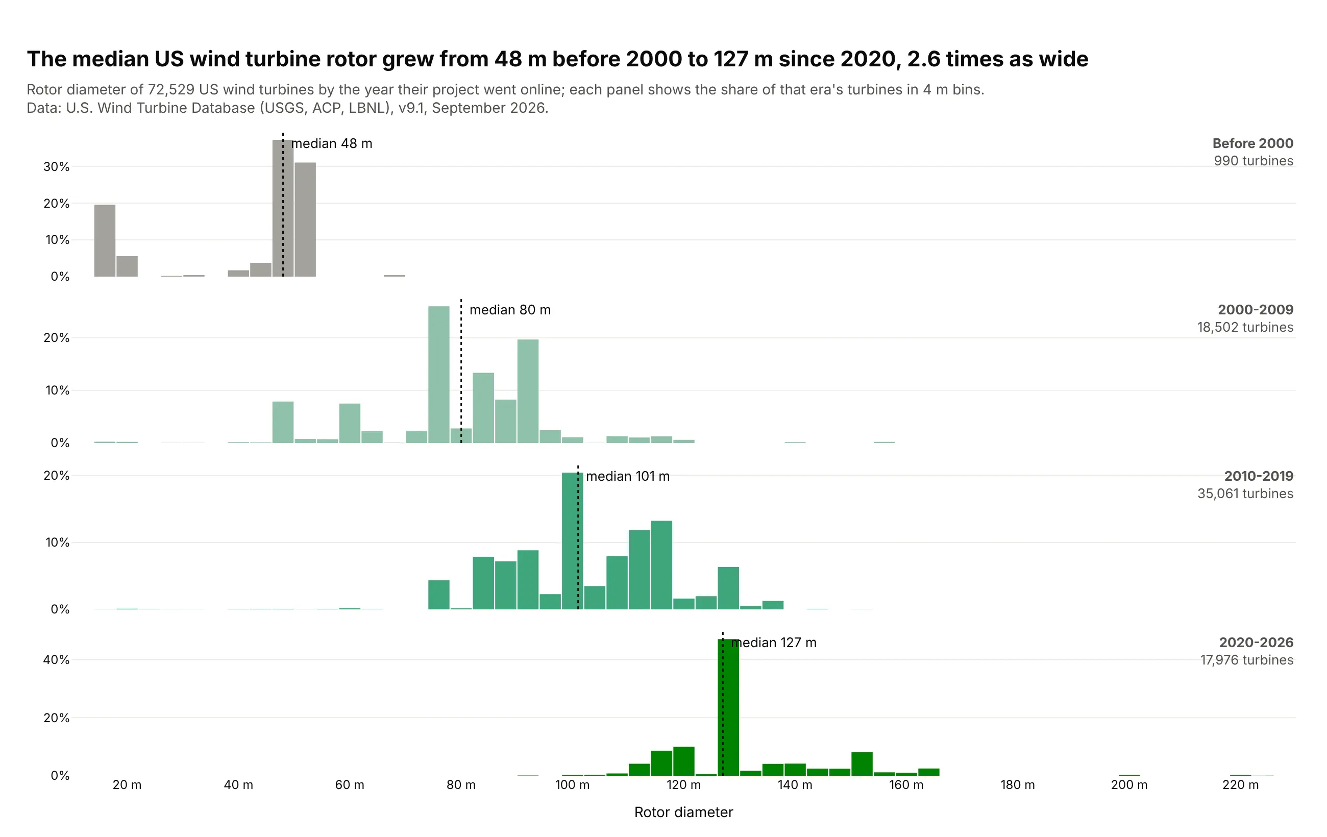
The median US wind turbine rotor grew from 48 m before 2000 to 127 m since 2020, 2.6 times as wide. Each era has a few dominant models, which show as tall single bins. Data: U.S. Wind Turbine Database v9.1 (doi:10.5066/F7TX3DN0).

Tip: small multiples on a shared x axis, with histnorm="percent" so the 990 early turbines read as clearly as the 35,061 from the 2010s.

3. Mortgages and the conforming loan limit

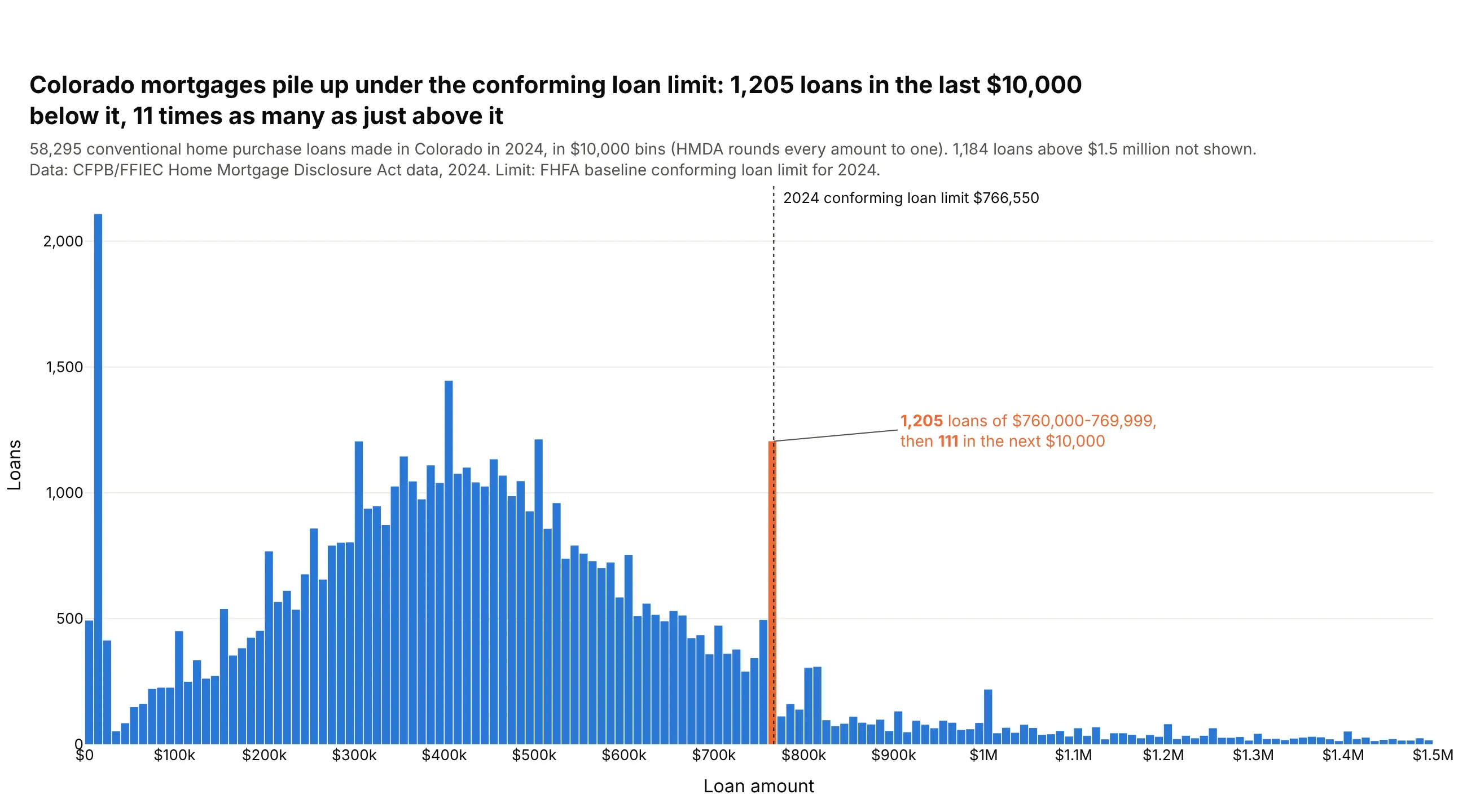
Colorado borrowers took 1,205 conventional purchase loans of $760,000-769,999 in 2024, just under the $766,550 conforming loan limit, and 111 in the next $10,000. In most counties, a bigger loan is a jumbo loan that Fannie Mae and Freddie Mac can't buy. Data: CFPB/FFIEC HMDA data, 2024.

Tip: $10,000 bins starting at $0, because HMDA rounds every amount to the middle of a $10,000 interval.

4. The size of every US bank

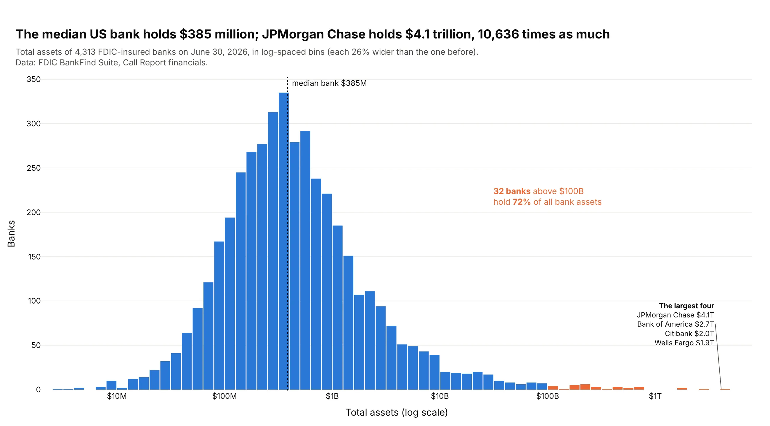
The median US bank holds $385 million; JPMorgan Chase holds $4.1 trillion, 10,636 times as much. The 32 banks above $100 billion hold 72% of all bank assets. Data: FDIC BankFind Suite, June 30, 2026.

Tip: histogram log10 of the values in 0.1 bins, then relabel the ticks in dollars.

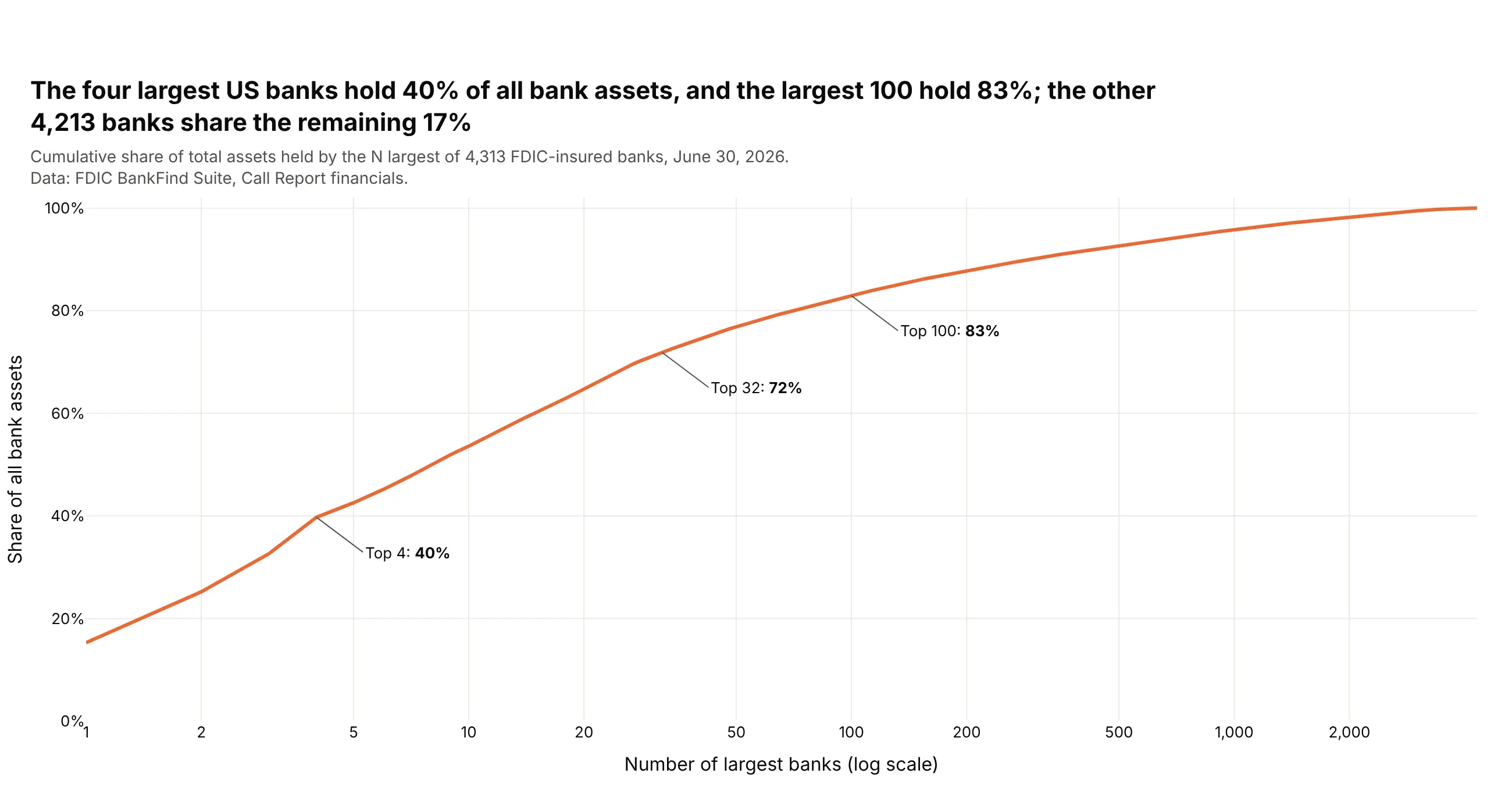
Another way to see it: the cumulative share of assets held by the largest N banks: the top 4 hold 40% and the top 100 hold 83%.

5. Height against weight for 5,970 adults

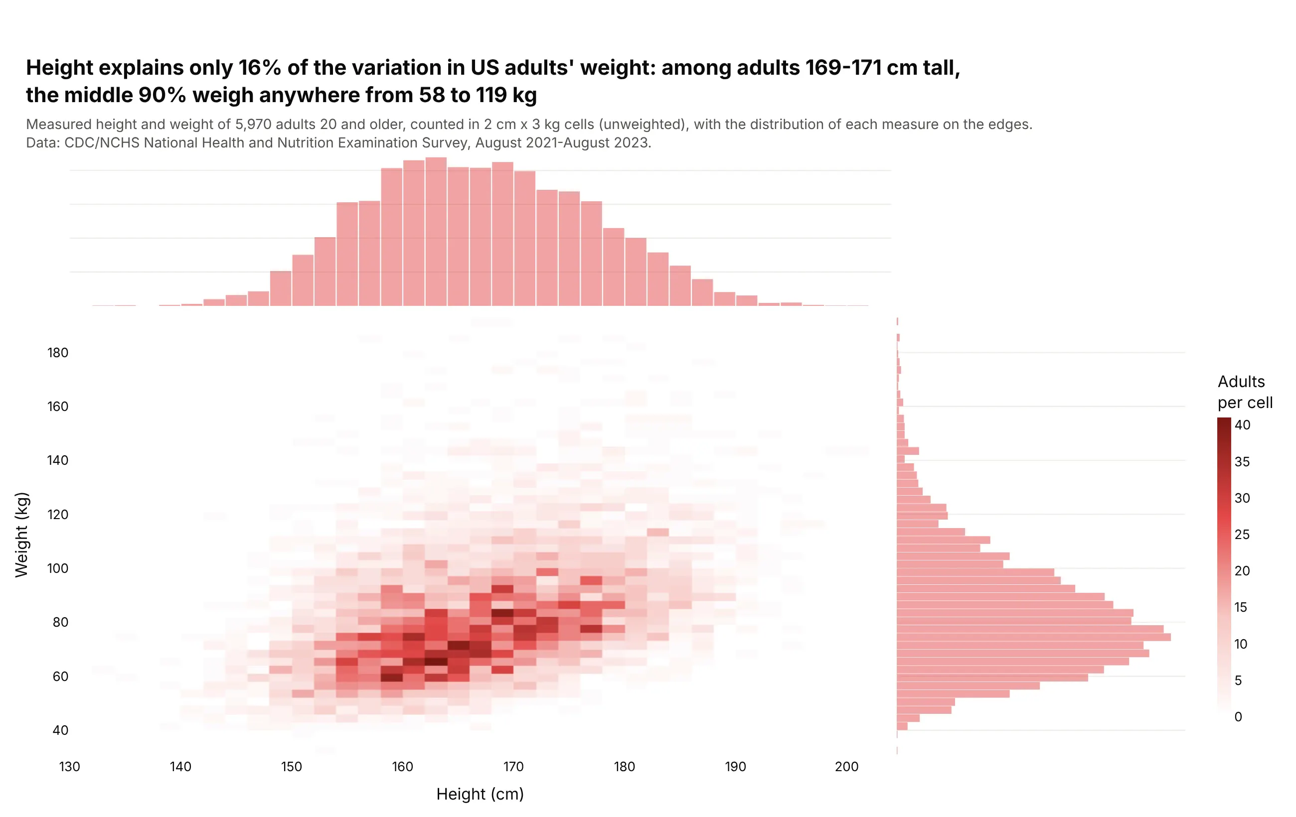
Height explains only 16% of the variation in US adults' weight. Among the 436 adults 169-171 cm tall, the middle 90% weigh anywhere from 58 to 119 kg. Data: CDC/NCHS NHANES, August 2021-August 2023.

Tip: px.density_heatmap with marginal_x and marginal_y="histogram" shows the joint and the single distributions together.

6. Weekday and weekend births

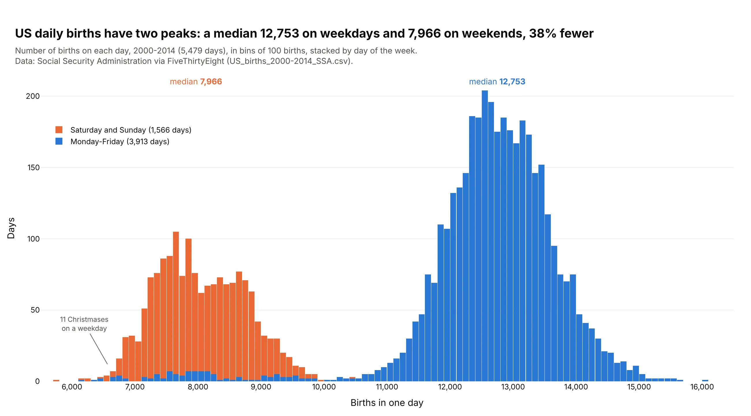
US daily births have two peaks: a median 12,753 on weekdays and 7,966 on weekends, 38% fewer, mostly because scheduled inductions and cesareans are booked on weekdays. Weekday holidays like Christmas fall in the weekend hump. Data: Social Security Administration via FiveThirtyEight, 2000-2014.

Tip: stack by day type, so the color explains the second peak.

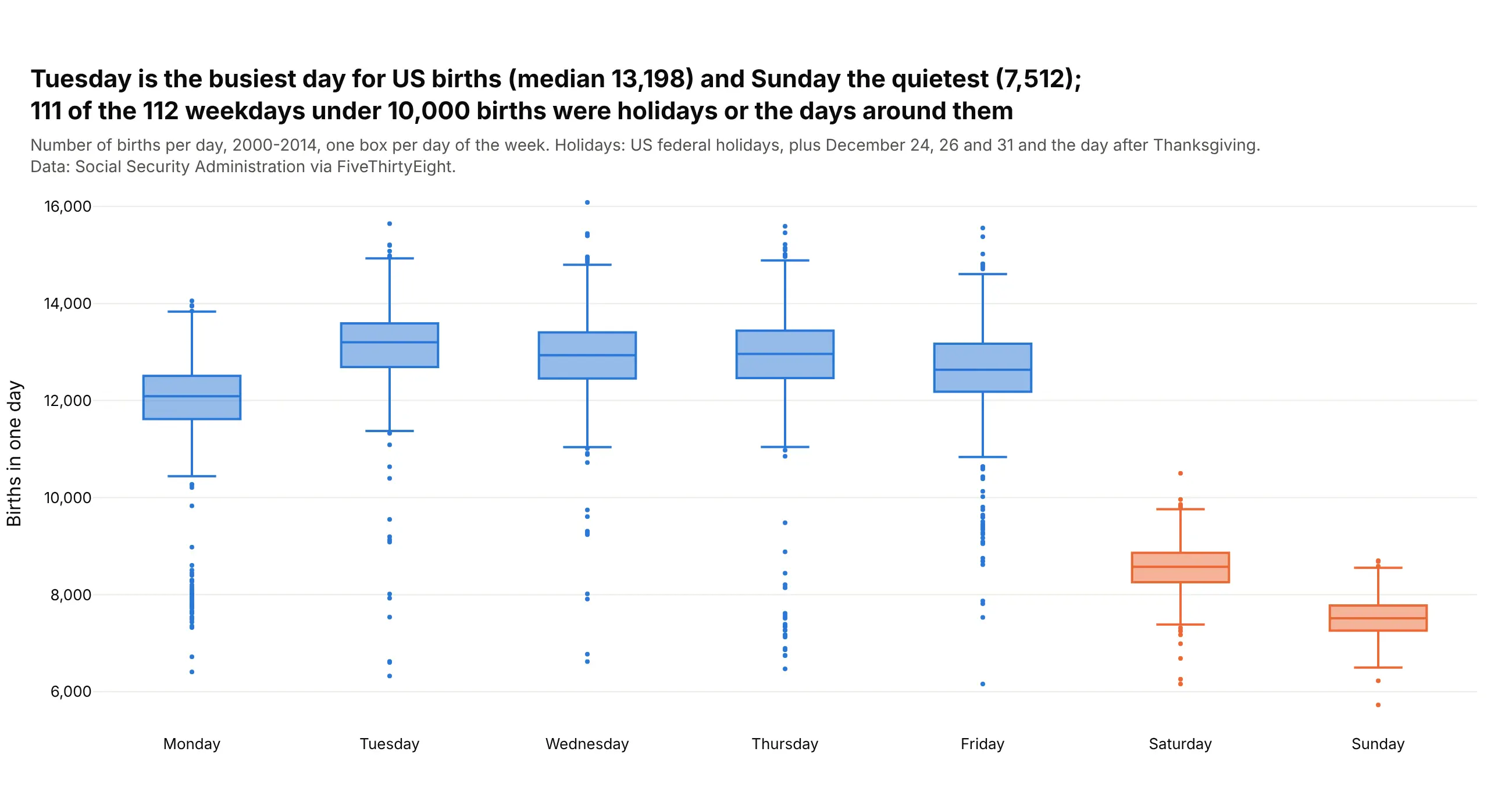
Another way to see it: one box per weekday shows Tuesday is busiest (median 13,198) and that 111 of the 112 weekdays under 10,000 births were holidays or the days around them.

7. How long clinical trials take to report results

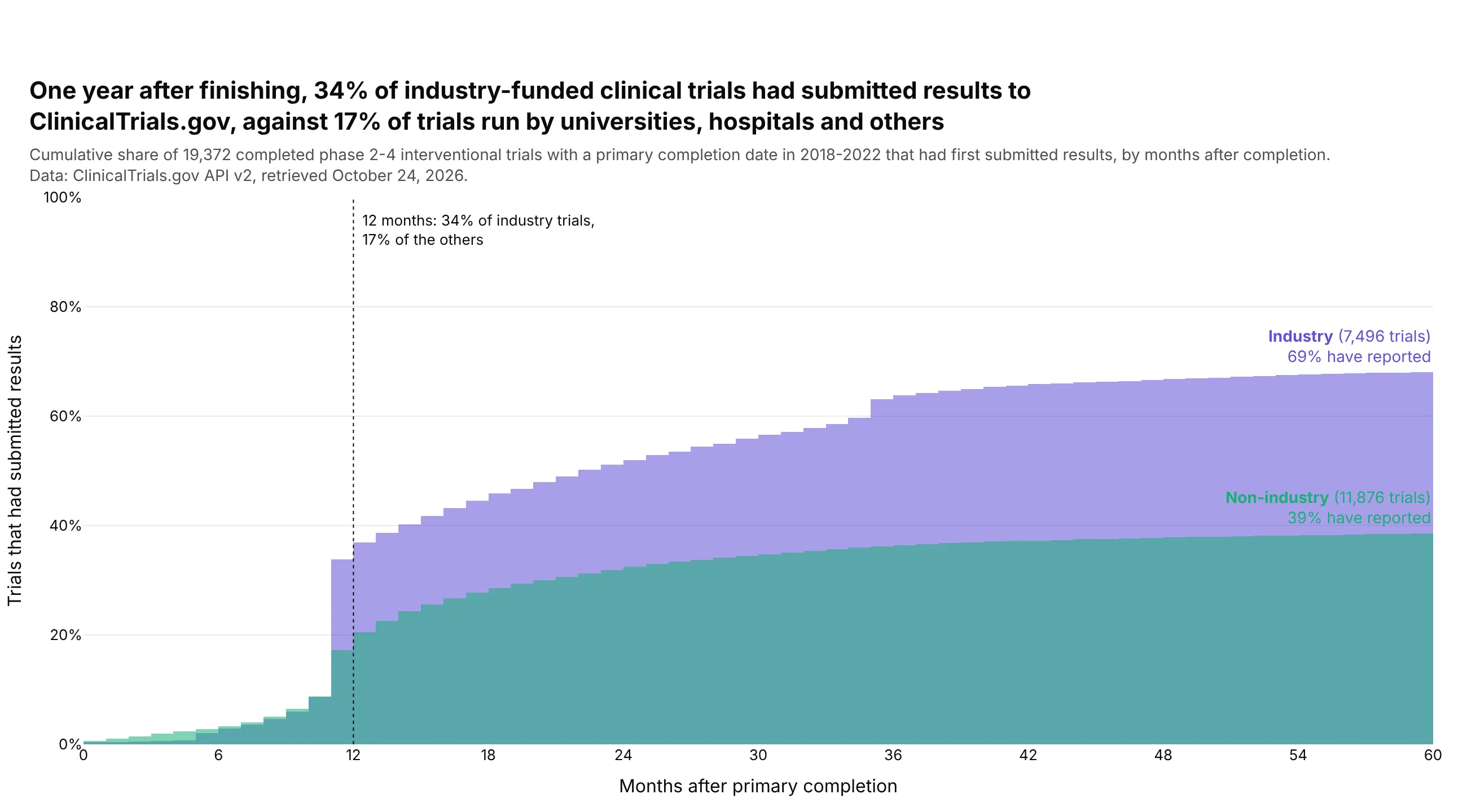
One year after finishing, 34% of industry-funded trials had submitted results to ClinicalTrials.gov, against 17% of trials run by universities, hospitals and others. After three years it's 63% and 36%. Data: ClinicalTrials.gov API v2, trials completed 2018-2022.

Tip: cumulative_enabled=True with trials that never reported placed beyond the axis, so curves level off at the true rate.

8. 1.9 million stars from Gaia

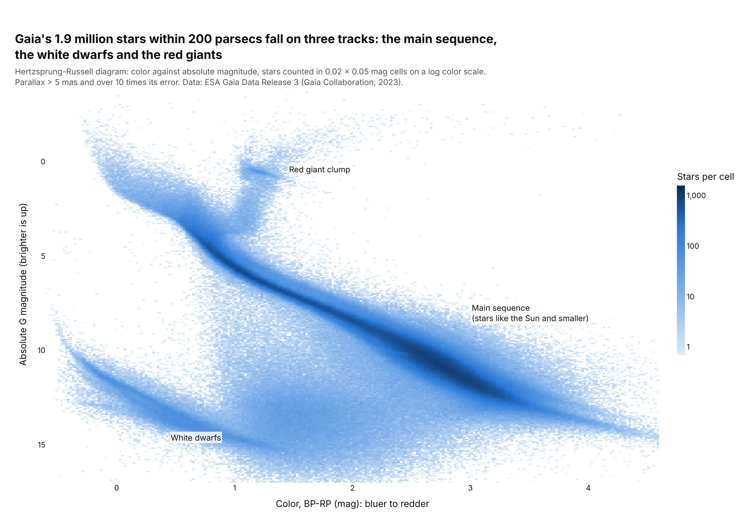
Gaia's 1.9 million stars within 200 parsecs fall on three tracks: the main sequence, the white dwarfs and the red giants. The archive counted the stars into 41,056 cells, so the CSV is 0.5 MB. Data: ESA Gaia DR3 (Gaia Collaboration, 2023).

Tip: go.Histogram2d on pre-binned cells with z = log10(count) + 1, so empty cells stay white.

9. Phoenix summers, then and now

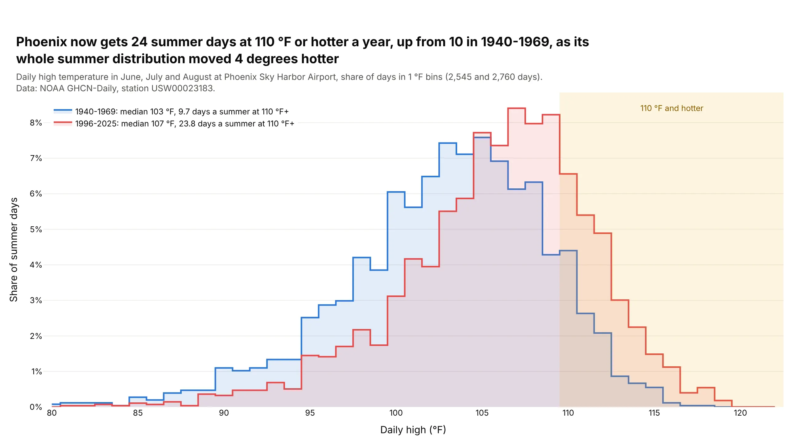
Phoenix now gets 24 summer days at 110 °F or hotter a year, up from 10 in 1940-1969. The median summer high moved from 103 °F to 107 °F. Data: NOAA GHCN-Daily, Phoenix Sky Harbor (Menne et al., 2012).

Tip: with integer data, center 1-degree bins on whole numbers, and draw step outlines (line_shape="hvh") instead of overlapping bars.

10. The ages of Congress

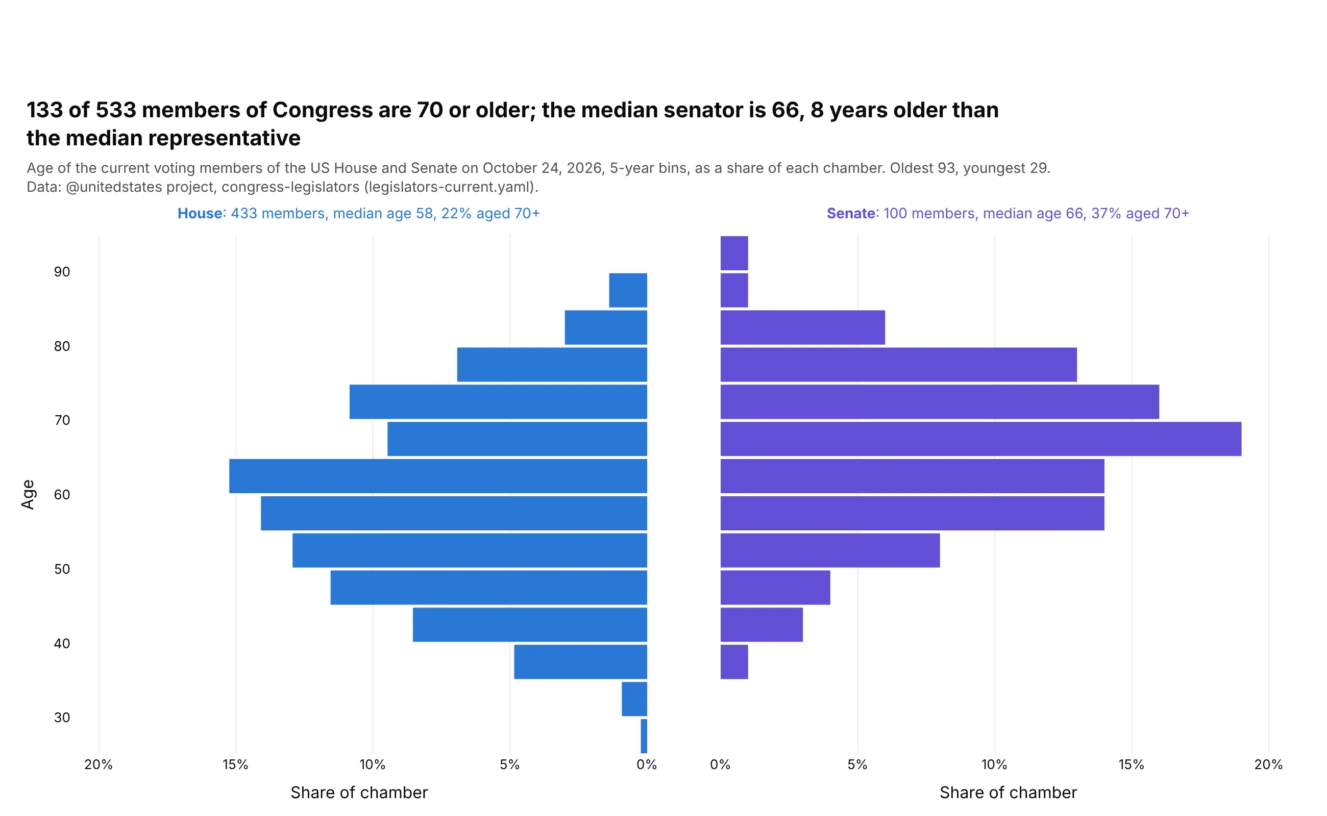
133 of the 533 voting members of Congress are 70 or older. The median senator is 66, 8 years older than the median representative, and 37% of senators are 70+ against 22% of the House. Data: @unitedstates project, congress-legislators, October 24, 2026.

Tip: two horizontal histograms in subplots that share the y axis, with the left x axis reversed, and histnorm="percent" for chambers of different size.

11. Old Faithful, the textbook bimodal distribution

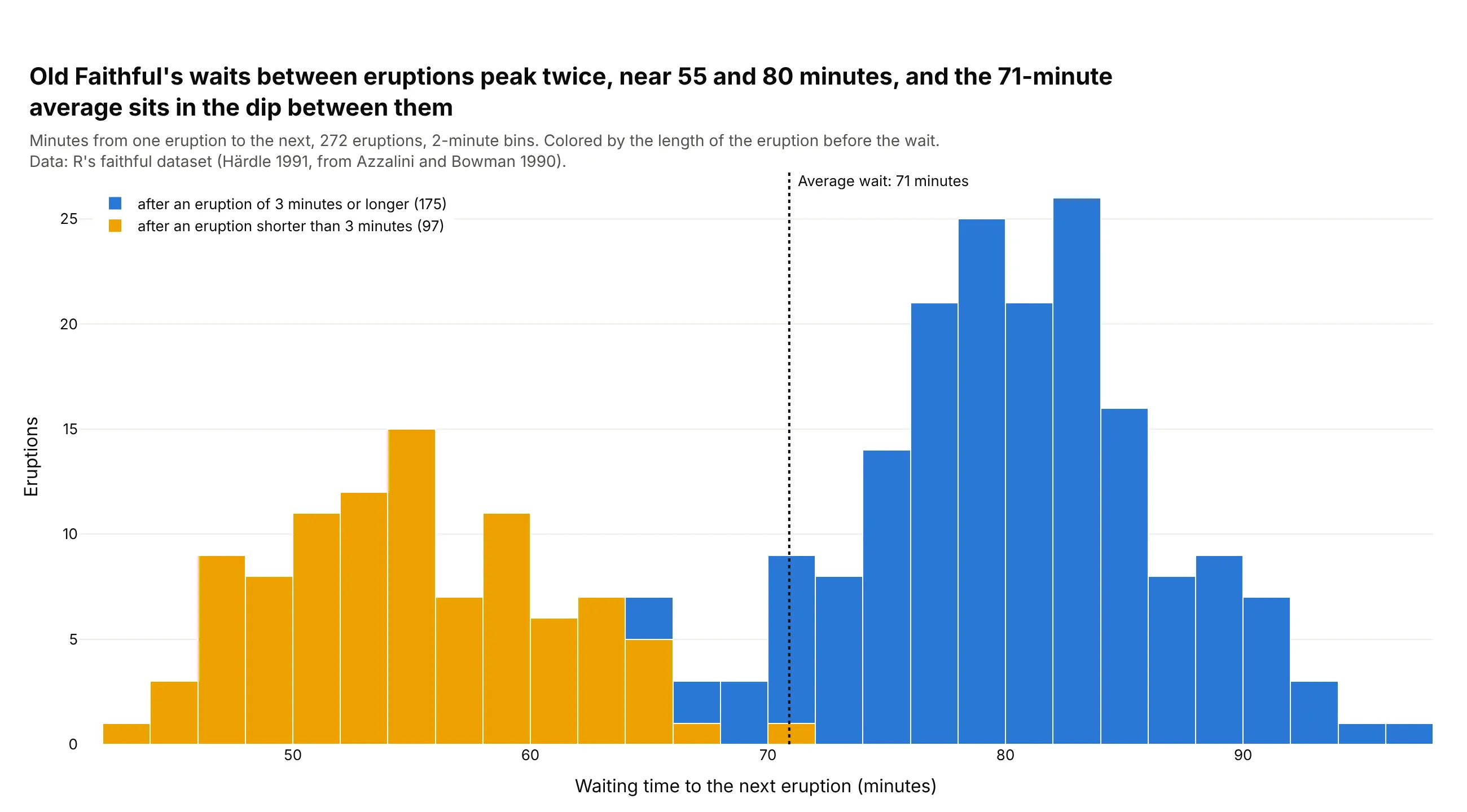
R ships the eruptions of the Old Faithful geyser in Yellowstone as its built-in faithful dataset, and seaborn ships the same data as geyser. The waits between eruptions have two peaks, because a short eruption is usually followed by a short wait: the median wait is 54 minutes after an eruption under 3 minutes and 80 after a longer one, so the 71-minute average sits in the dip between them, where few waits fall. Data: R's faithful dataset (Härdle, 1991, from Azzalini and Bowman, 1990).

Tip: color the bars by a second variable with a stacked go.Histogram per group, which shows what splits the distribution, and mark the mean to show why one average misleads.