Chris Parmer

October 24, 2026

ECDF Plots - A Complete Guide (with 14 Examples)

TL;DR

An ECDF plot draws every value in a dataset as one step up a curve, so the height at any x is the share of values at or below x.
ECDF plots are also known as empirical cumulative distribution function plots and empirical CDF plots, and are similar to histograms and Kaplan-Meier curves.
Use one to compare distributions without choosing bins, and to read medians, percentiles and "share above a threshold" straight off the chart.
Flipped, it becomes the complementary ECDF (share above x), which energy and water engineers call a duration or exceedance curve.
In Python it's one line of code: px.ecdf(df, x="value", color="group"). The 14 examples below come with a prompt you can paste into Plotly Studio or any AI tool.

What is an ECDF plot?

ECDF plots look like this:

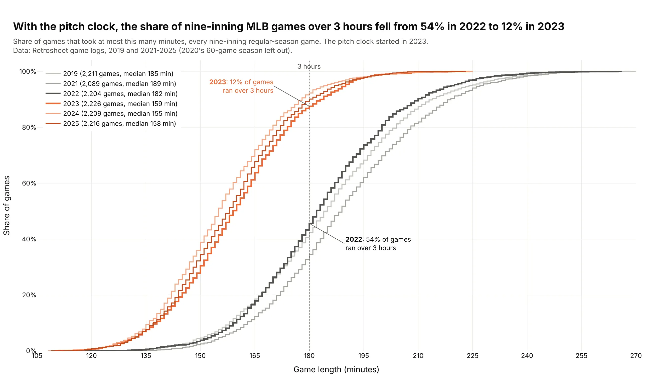
ECDF plot of every nine-inning MLB game length from 2019 to 2025, one step line per season. The 2019, 2021 and 2022 curves sit to the right in grays with medians of 185, 189 and 182 minutes; the 2023, 2024 and 2025 curves sit further left in oranges with medians of 159, 155 and 158 minutes. At the 3-hour line, 54% of 2022 games ran longer, against 12% in 2023

Data: Retrosheet game logs, 2019 and 2021-2025.

How do you read an ECDF plot? In the example above, notice these things:

Each line is one season, and it climbs one small step for every game, from the shortest game on the left to the longest on the right. The height of a line at any game length is the share of that season's games that took that long or less.
To check a threshold, go up from the x axis to a curve. At the dashed 3-hour line the dark gray 2022 curve is just under halfway up, so more than half of that season's games ran longer than 3 hours.
To find a median, go across from 50% on the y axis. The horizontal gap between the dark gray 2022 curve and the orange 2023 curve there means the typical game got 23 minutes shorter in the first season with a pitch clock.
Six seasons fit on one chart because an ECDF has no bins, while six histograms would overlap into a mess and each would change shape with the bin width you pick. The gray curves are the seasons before the pitch clock and the orange ones the seasons after it, and the three orange curves lie almost on top of each other, so the change held in 2024 and 2025.
A curve that sits higher or further left means shorter games, which is the opposite of how most line charts read. The lightest orange curve, 2024, is the highest of the six for almost every game length, and its median game was the shortest.

It's often used for charts like these:

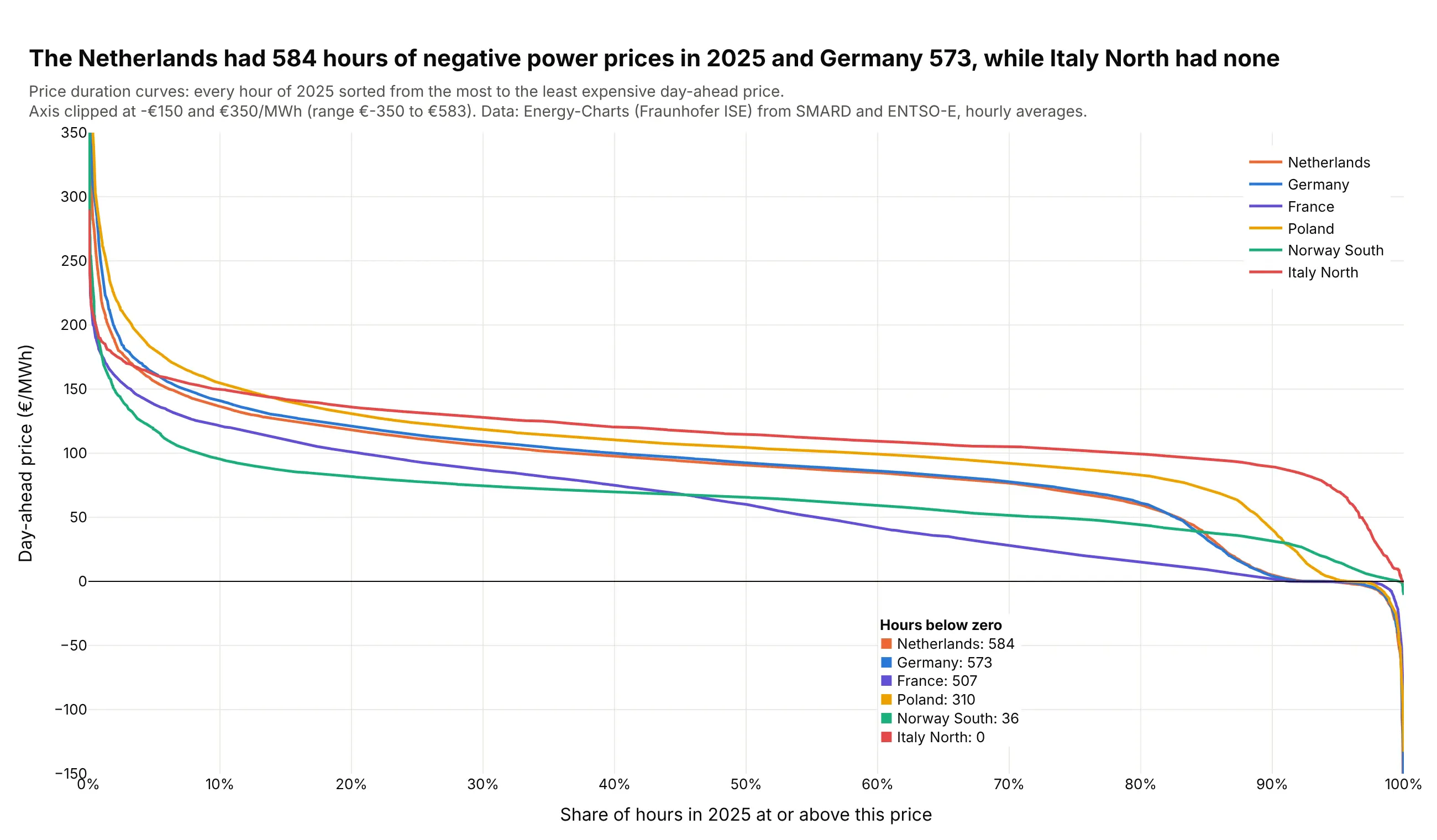
Price duration curves for six European power markets in 2025, each hour of the year sorted from the most to the least expensive day-ahead price. The Netherlands (584 hours), Germany (573) and France (507) dip below zero at the right end, while Italy North never does

Duration curves in energy. Sorting every hour of 2025 by price shows that the Netherlands had 584 hours of negative day-ahead power prices and Italy North none. Data: Energy-Charts (Fraunhofer ISE), from SMARD and ENTSO-E.

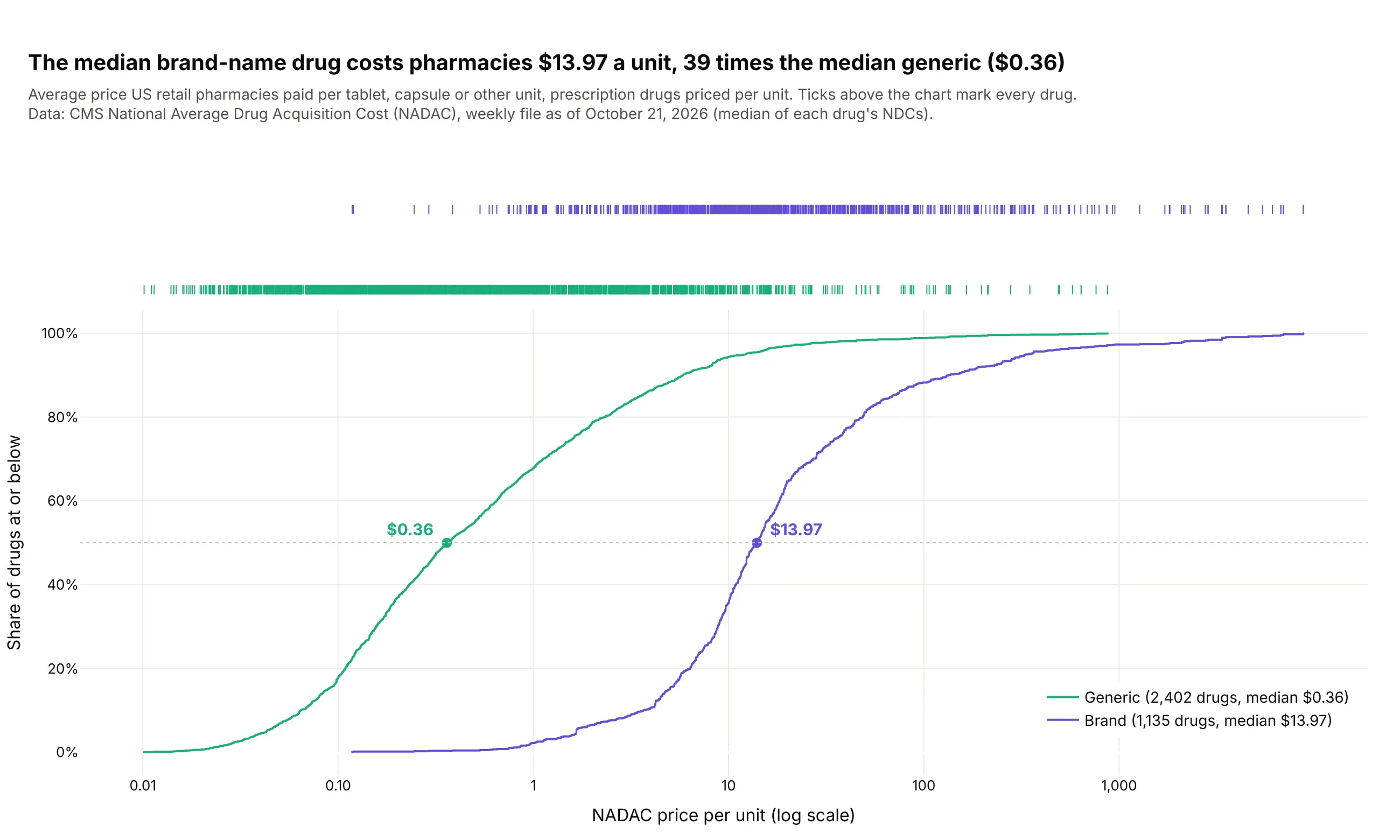
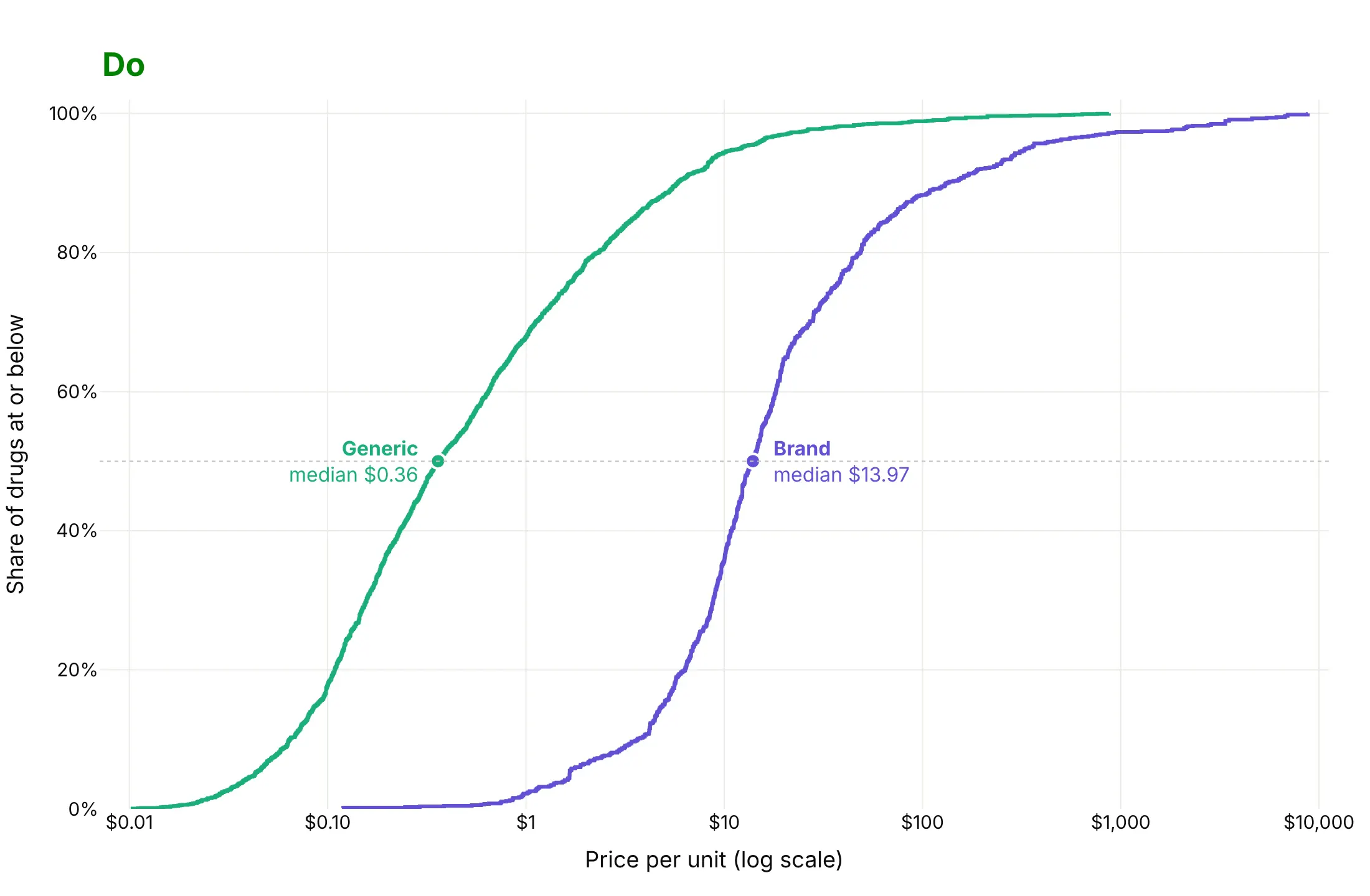
Comparing groups on a log scale. The median brand-name drug costs pharmacies $13.97 a unit, 39 times the median generic at $0.36. Data: CMS National Average Drug Acquisition Cost (NADAC), October 2026.

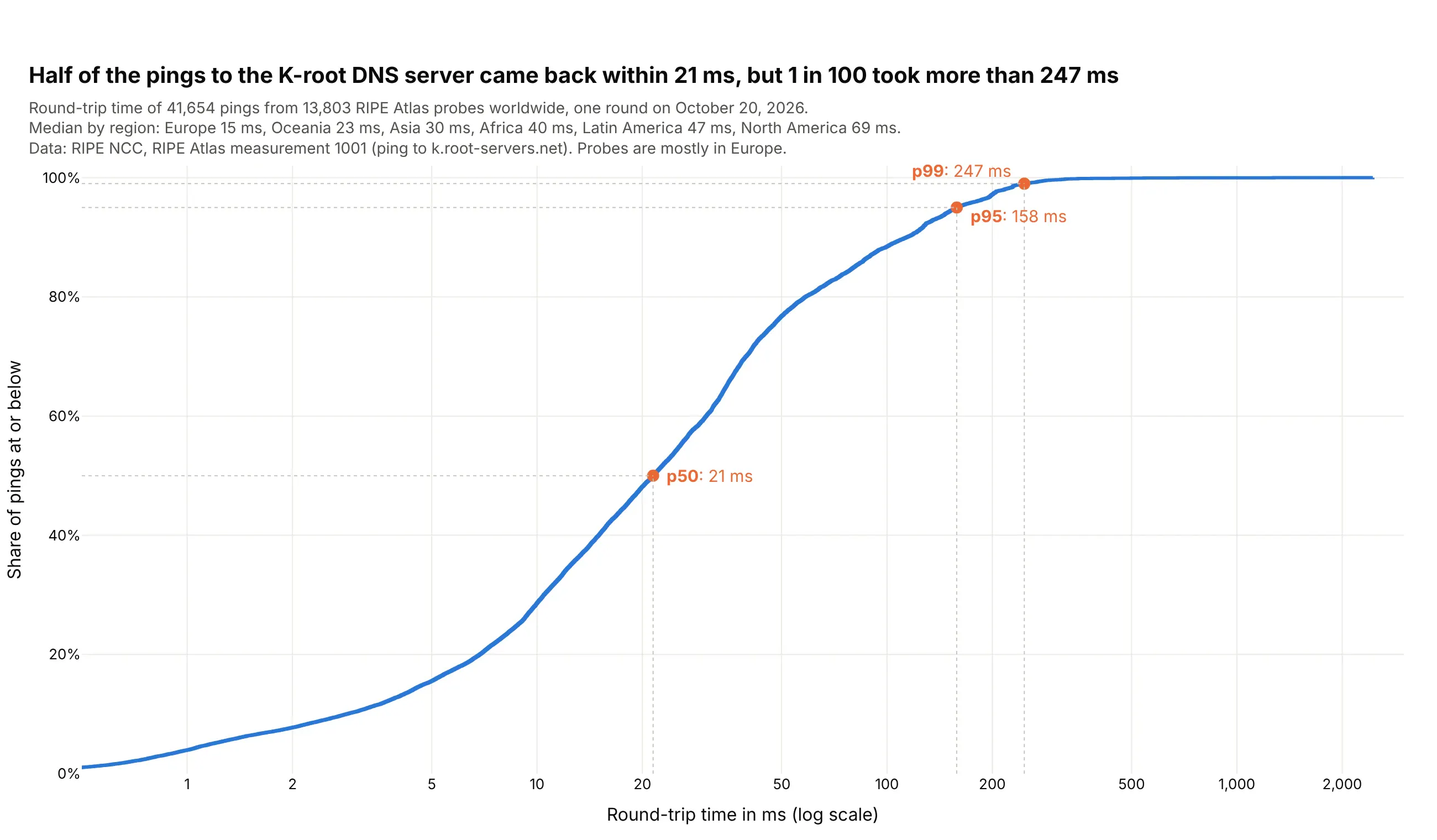
ECDF of 41,654 ping times from 13,803 RIPE Atlas probes to the K-root DNS server on a log axis, with p50 at 21 ms, p95 at 158 ms and p99 at 247 ms marked

Latency percentiles. Half of the pings to the K-root DNS server came back within 21 ms, but 1 in 100 took more than 247 ms. Data: RIPE Atlas measurement 1001, October 20, 2026.

A short history

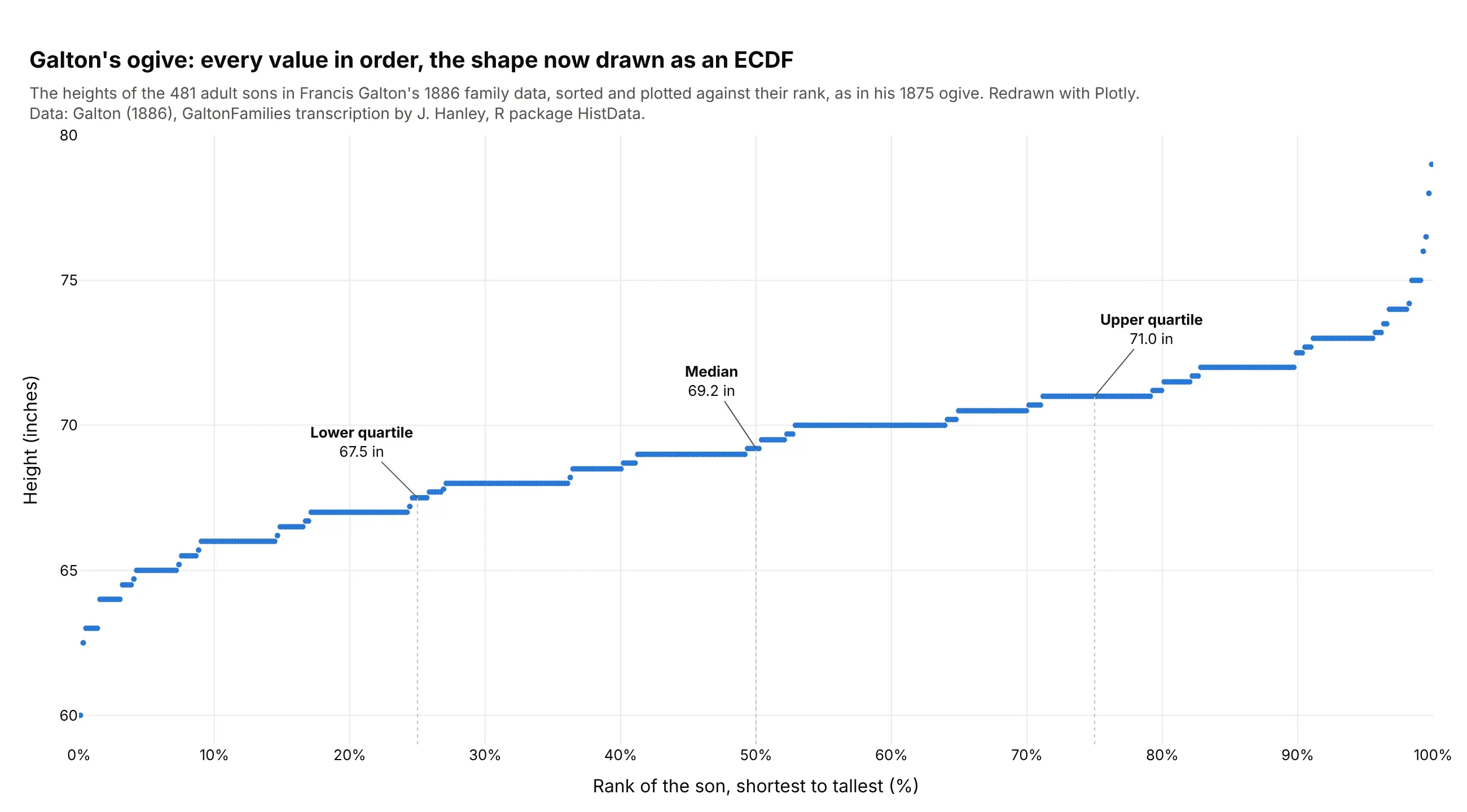
Francis Galton described the "ogive" in 1875: line up every value in order and draw each one against its rank (Galton, 1875). That is an ECDF with the axes swapped, and it let him read the median and quartiles off a curve. Here it is on the heights of the 481 adult sons in his 1886 family data (Galton, 1886):

Galton's ogive redrawn with Plotly: the heights of 481 sons from his 1886 family data sorted from shortest to tallest, from 60 to 79 inches, with the lower quartile at 67.5 inches, the median at 69.2 and the upper quartile at 71.0

Statisticians later proved that the ECDF converges to the true distribution as the sample grows, and Dvoretzky, Kiefer and Wolfowitz bounded how far from it the ECDF can be for any sample size (1956), which gives the band in example 2 below.

Alternatives to an ECDF plot

Here's the same 4,430 MLB games drawn six ways. Some are better for the question, some worse, some just different:

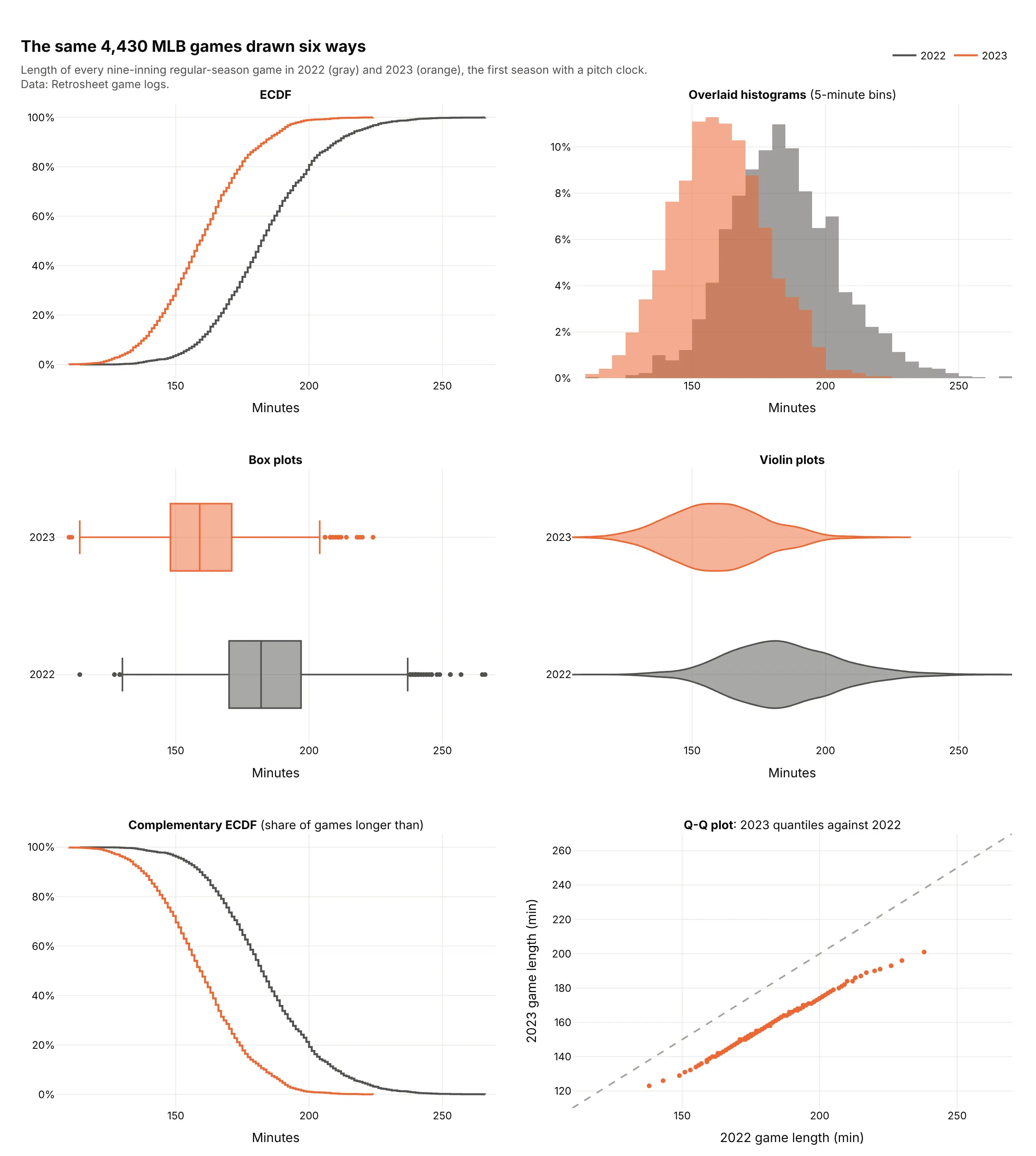
The same nine-inning MLB game lengths for 2022 and 2023 as an ECDF, overlaid histograms with 5-minute bins, box plots, violin plots, a complementary ECDF and a Q-Q plot of 2023 quantiles against 2022 that sits 15 to 37 minutes below the diagonal

Histogram (better for the shape). Peaks, gaps and skew are easier to see as bars, and most readers know how to read one. Two overlapping histograms are harder to compare than two ECDFs, and the picture changes with the bin width.
Box plot (works too, for many groups). Five numbers per group fit dozens of groups side by side, but the box hides everything between the quartiles. See our box plot guide.
Violin plot (different). A smoothed shape per group, good for spotting two peaks, with a smoothing bandwidth to choose instead of bins. See our violin plot guide.
Complementary ECDF (different). The same curve flipped to show the share above each value, which suits risk, exceedance and survival questions (examples 3, 4 and 7).
Q-Q plot (better for comparing two distributions in detail). Matching percentiles of 2023 against 2022 fall 15 to 37 minutes below the diagonal, so every part of the distribution got shorter and the longest games lost the most time.

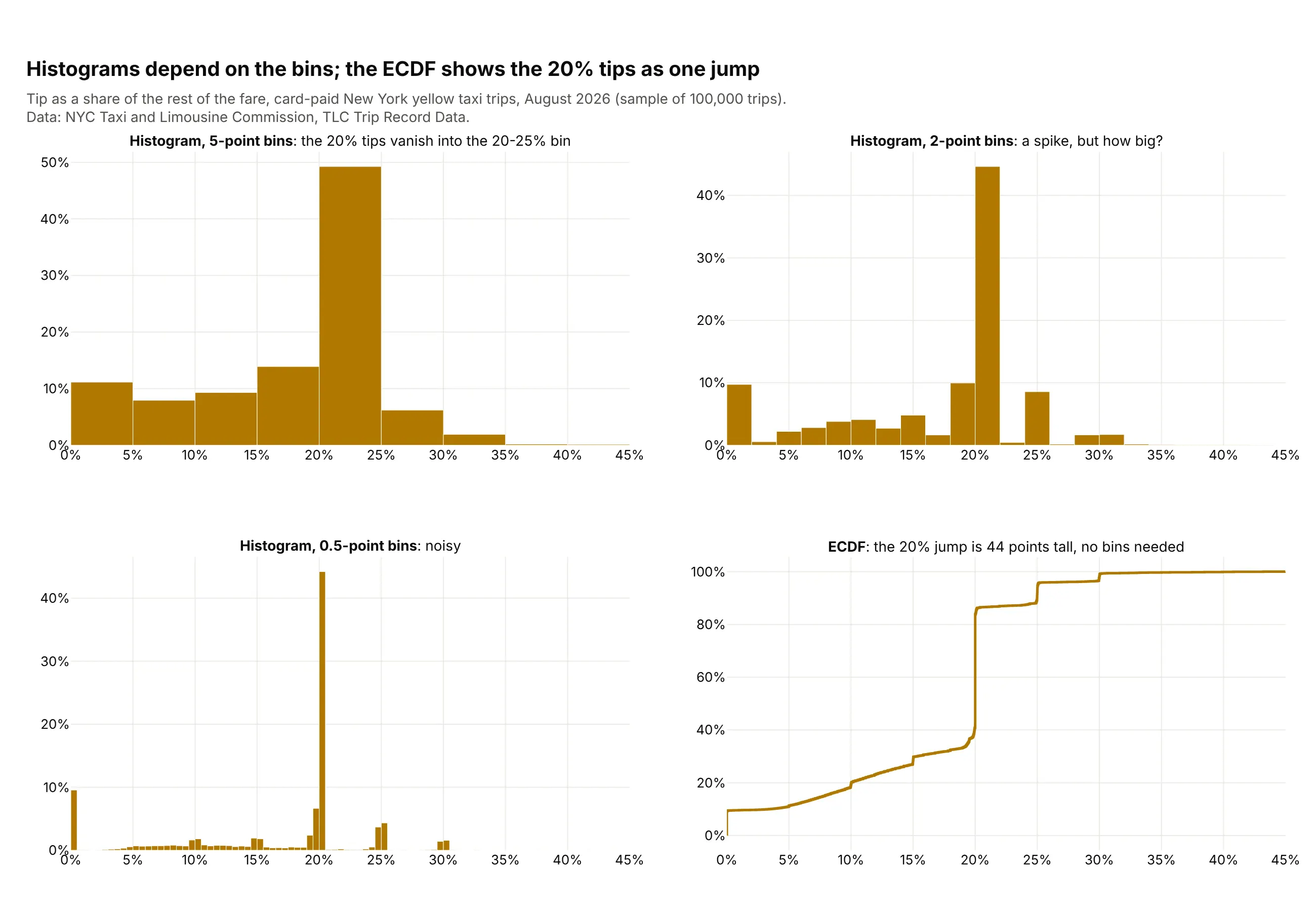
Here's where the ECDF wins. Taxi tips cluster at round numbers, and a histogram shows that or hides it depending on the bins, while the ECDF shows the 20% tips as one 44-point jump:

The same 100,000 New York taxi tips as histograms with 5-point, 2-point and 0.5-point bins and as an ECDF. The 5-point histogram merges the 20% tips into a 20-25% bar, the 2-point one shows a spike, the 0.5-point one is noisy, and the ECDF shows a vertical jump of 44 points at 20%

How to make an ECDF plot

With AI

ChatGPT, Claude Code, GitHub Copilot, Cursor and other AI tools are excellent at writing Plotly code. Name Plotly in the prompt, say which column holds the values and which one splits the groups, and list the checks you want:

Make a plotly ECDF plot from latency.csv (columns: service, region, latency_ms).

- One step line per service with px.ecdf, colored by service, on a log x axis.
- Y axis as a percent: "Share of requests at or below".
- Mark p50, p95 and p99 of each service with a dot and a label.
- If a service has more than 100,000 rows, draw 1,000 quantiles instead of every row.
- Put the source in a muted subtitle and a title that states the main takeaway.
- Print each service's p50, p95 and p99 so I can check the labels.
- Save it as ecdf.html and as a PNG at 2x scale.

With Plotly Studio

Plotly Studio is a desktop app where you point an AI at a dataset and it builds charts and a Dash app around your questions. Ask for an ECDF the same way:

Show an ECDF of hourly power prices for each market, with a dropdown to switch between the standard curve and a price duration curve, and a slider that sets a price threshold and shows the share of hours above it.

Make an ECDF plot in Python or JavaScript

This is the code AI tools write under the hood. Plotly Express has an ECDF function, which sorts the values and draws them as a step line:

import plotly.express as px

df = px.data.tips()
fig = px.ecdf(df, x="total_bill", color="time")
fig.update_layout(yaxis_tickformat=".0%")
fig.show()

px.ecdf sends every row to the browser. For a weighted, flipped or very large ECDF, it's easier to build the step line yourself, and this helper draws 1,000 quantiles when there are more values than that:

import numpy as np
import plotly.graph_objects as go


def ecdf_trace(values, name, max_points=1000, complementary=False):
    v = np.sort(np.asarray(values, dtype=float))
    if len(v) > max_points:
        y = np.linspace(0, 1, max_points)
        x = np.quantile(v, y)
    else:
        x, y = v, np.arange(1, len(v) + 1) / len(v)
    if complementary:
        y = 1 - y
    return go.Scatter(x=x, y=y, mode="lines", line_shape="hv", name=name)

In JavaScript, you make an ECDF with plotly.js by sorting the values and drawing them as a step line:

<div id="chart"></div>
<script src="https://cdn.plot.ly/plotly-4.1.1.min.js"></script>
<script>
  const values = [12, 7, 3, 25, 9, 14, 7, 31, 5, 11];
  const x = [...values].sort((a, b) => a - b);
  const y = x.map((_, i) => (i + 1) / x.length);
  Plotly.newPlot("chart", [{
    type: "scatter", mode: "lines", line: {shape: "hv"}, x: x, y: y
  }], {yaxis: {tickformat: ".0%", title: {text: "Share at or below"}}});
</script>

Share it

Every Plotly chart has a Share chart button (the cloud icon in its toolbar) that uploads it to Plotly Cloud and gives you a link. Only you can see it until you change its visibility.

For a live app, put the chart in a Dash app and publish it with the Plotly Cloud CLI. Coding agents can run these commands for you:

pip install "dash[cloud]"
plotly user login
plotly app publish

If your data has to stay in your own cloud or data center, publish to Dash Enterprise instead.

Dos and don'ts

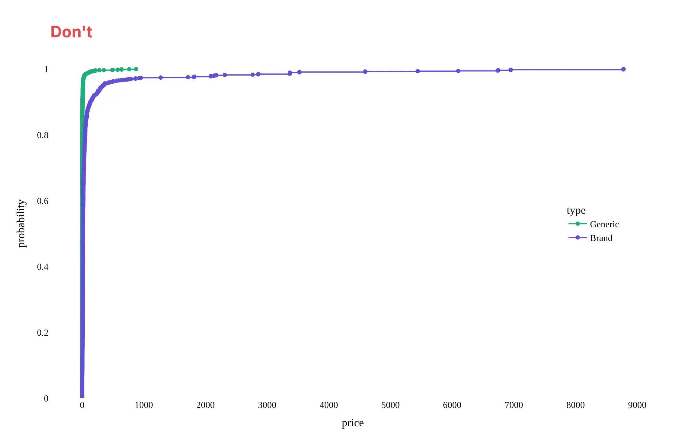
Here are the same 3,537 drug prices both ways, with the same colors. The difference is in the axis, the marks and the labels.

Don't use a linear axis for values that span six orders of magnitude, put a marker on every one of 3,537 points, or leave raw column names, unformatted ticks and a serif font:

Do use a log axis with dollar ticks, draw plain step lines, and mark and label the medians where the curves cross 50%:

Choose what the y axis shows

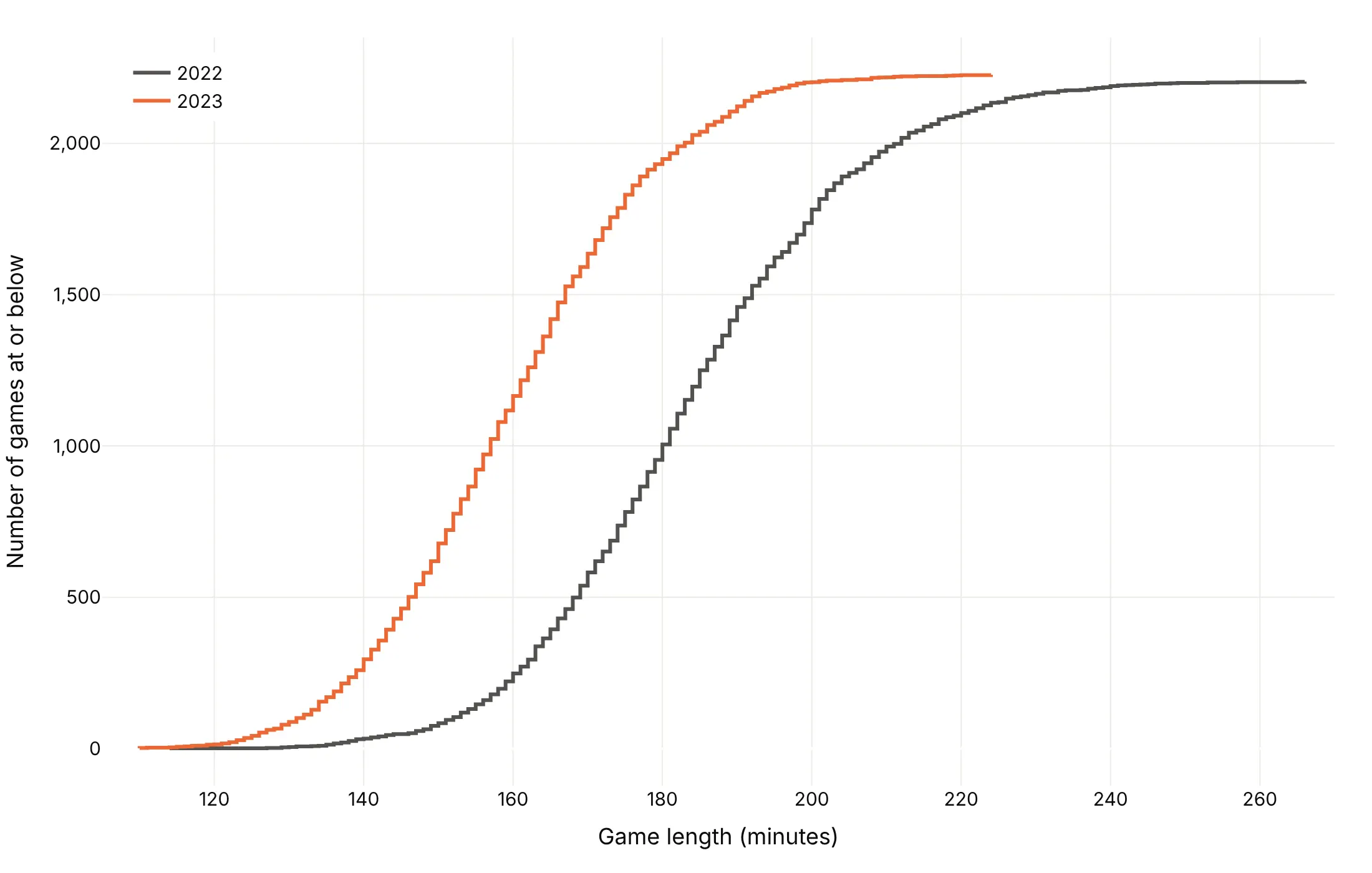
The same curve can answer three questions. Here are the 2022 and 2023 MLB seasons each way.

Share at or below (the default, ecdfnorm="probability"). Best for percentiles and medians.

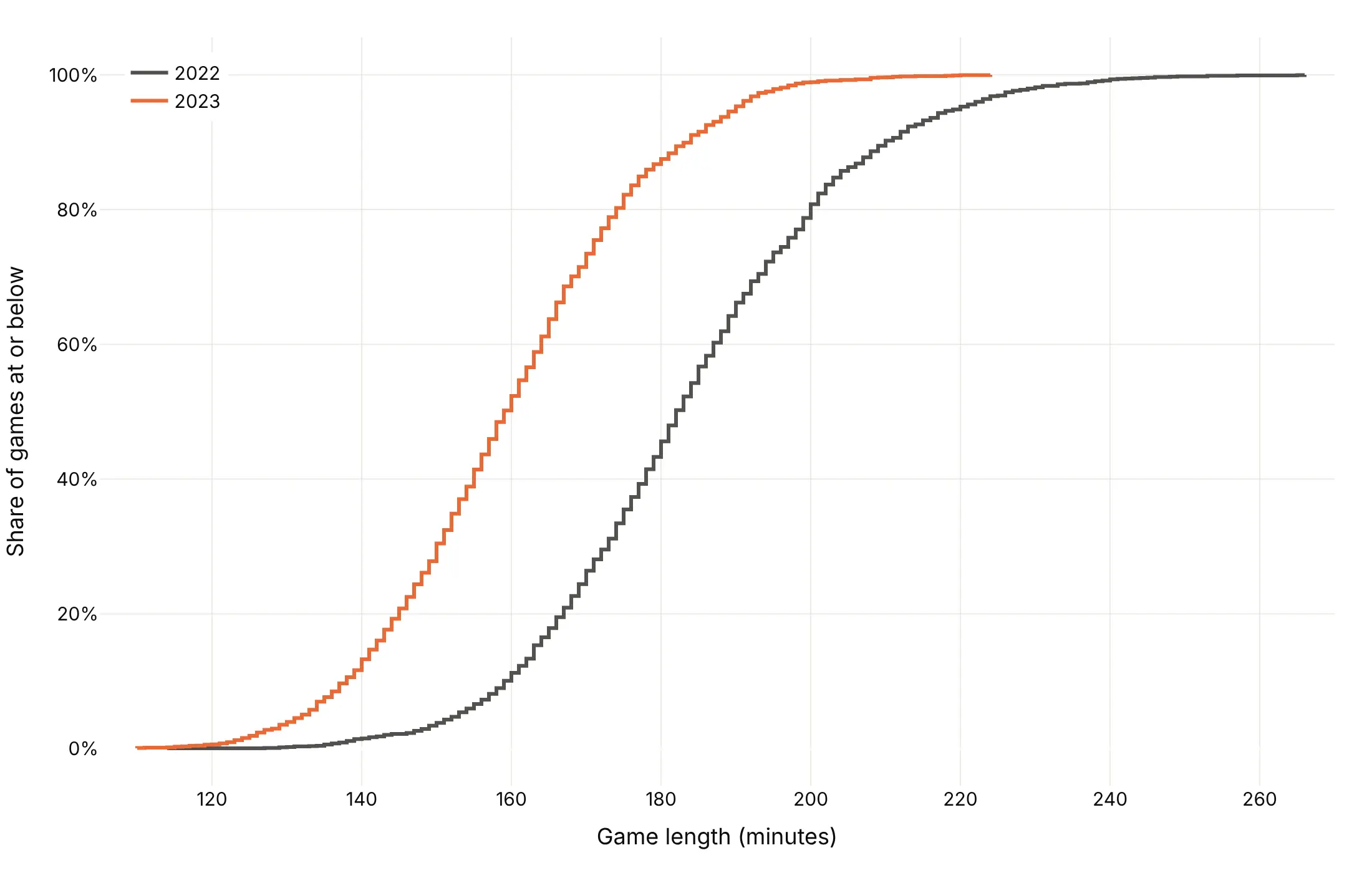
ECDF of 2022 and 2023 nine-inning MLB game lengths with the y axis as the share of games at or below each length

Share above (ecdfmode="complementary"). Best for risk, exceedance and "how many took longer than".

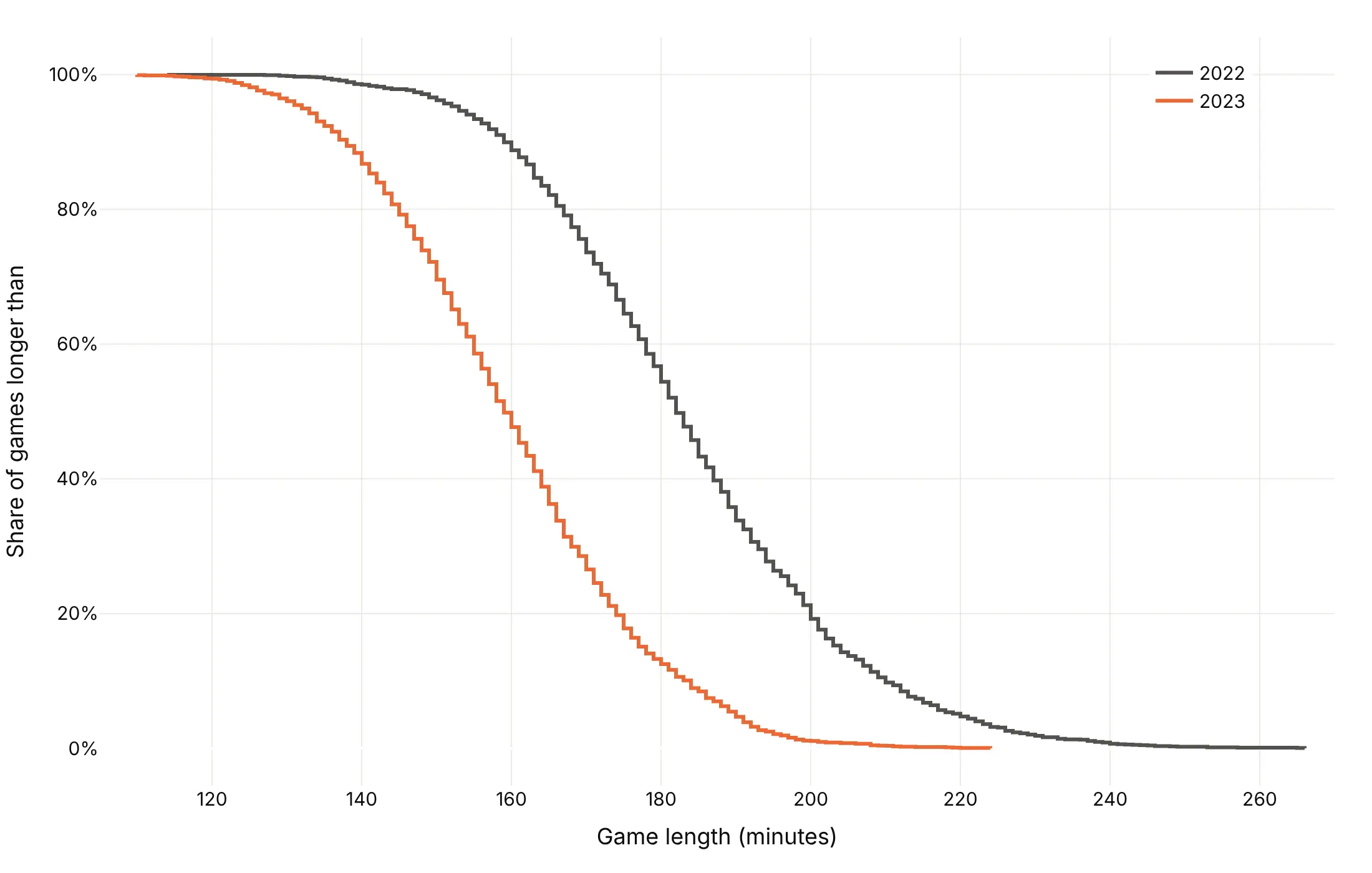
The same two seasons as complementary ECDFs, falling from 100% to 0%, with the y axis as the share of games longer than each length

Counts (ecdfnorm=None). Best when the totals differ and matter, such as earthquakes per year (example 9).

The same two seasons with the y axis as the number of games at or below each length, ending at 2,204 games for 2022 and 2,226 for 2023

Checklist

Write a title that states the takeaway with a number read off the curve.
Use a log x axis for prices, sizes, latencies and flows.
Draw a reference line at a threshold or at 50%, and label where each curve crosses it.
Label curves directly or in a legend that holds the key numbers.
Say in the subtitle whether the y axis is the share at or below, the share above, or a count.

Don't

Put markers on thousands of points; use them only for small samples (example 2).
Smooth the steps away with a spline, because each jump is real data.
Send millions of raw points to the browser; draw quantiles instead.
Compare groups of very different sizes without giving each group's count.

Options to customize

These are the px.ecdf arguments and go.Scatter attributes that matter most for an ECDF. The full list is in the Plotly ECDF documentation.

x: the column of values. Pass y instead for a horizontal ECDF.
y with x: a weight column, so each value counts by its weight, such as megawatts instead of plants (example 1).
color: one curve per group.
ecdfnorm: "probability" (default, 0 to 1), "percent" (0 to 100) or None for counts.
ecdfmode: "standard" (at or below), "complementary" (above) or "reversed" (at or above).
markers: a dot on every value, for small samples.
marginal: "rug", "histogram", "box" or "violin" above the plot.
log_x, log_y: log axes, for skewed values or tails.
facet_col, facet_row: small multiples instead of overlapping curves.
render_mode: "svg" or "webgl"; "auto" switches to WebGL above 1,000 rows.
line_shape="hv" (go.Scatter): the step line. "vh" steps the other way, as ecdfmode="reversed" does.
fill="tonexty" (go.Scatter): a shaded band between two curves, such as a confidence band.
yaxis.tickformat=".0%" (layout): shares as percents.
add_hline, add_vline: reference lines at 50% or at a threshold.

More ECDF plot examples

Ten more ECDF plots built from real public data, each with its source, the technique that makes it work and a prompt to rebuild it.

1. Most US solar plants are small, but most solar capacity is in big plants

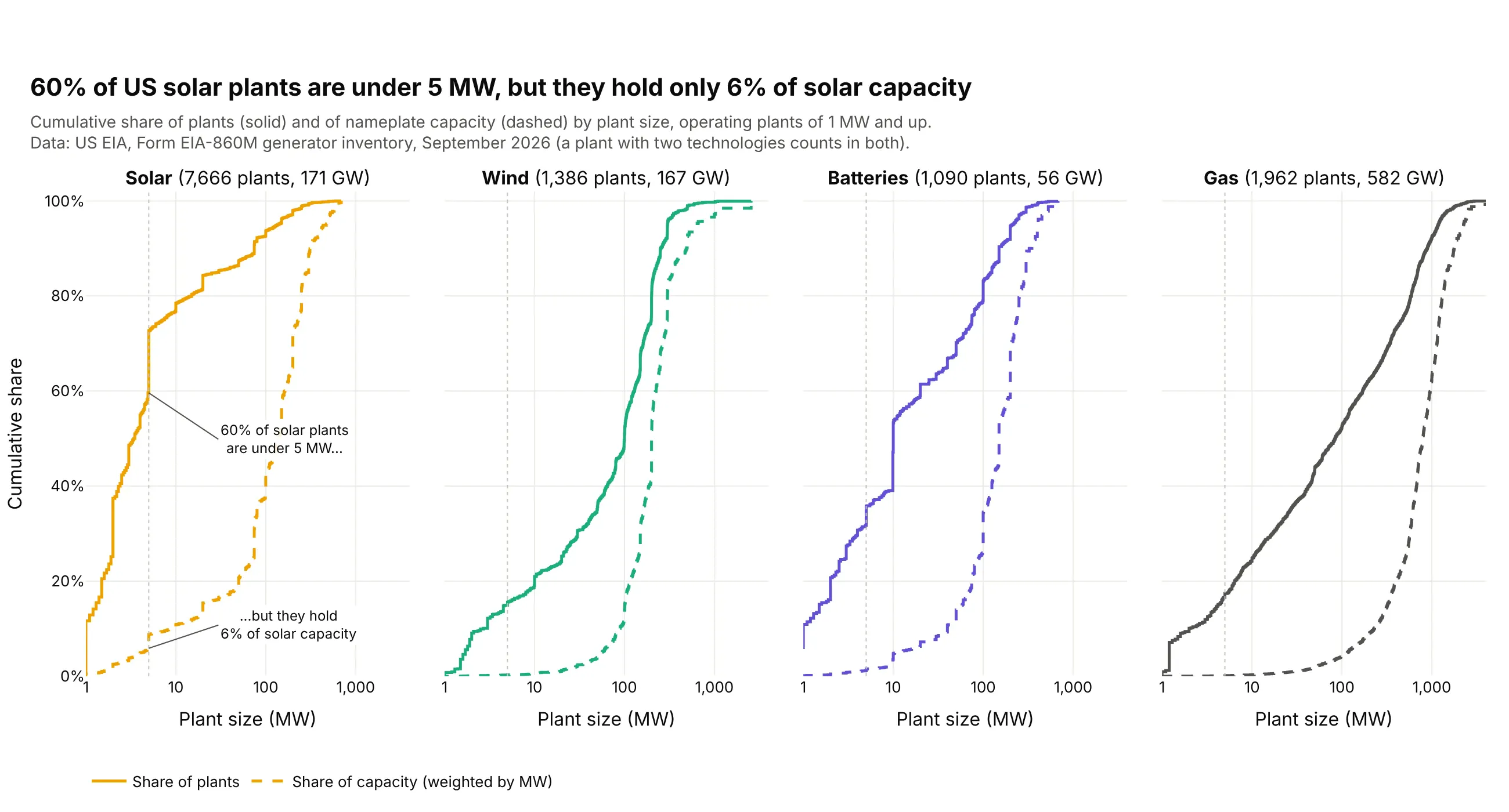
Four panels of ECDFs for US solar, wind, battery and gas plants on a log axis of plant size, each with a solid curve for the share of plants and a dashed curve for the share of capacity. For solar, 60% of plants are under 5 MW but they hold 6% of solar capacity

Each panel has two ECDFs of the same plants, one counting plants and one weighted by megawatts. 60% of the 7,666 US solar plants are under 5 MW, but they hold only 6% of the 171 GW of solar capacity. Data: US EIA, Form EIA-860M generator inventory, September 2026.

Tip: passing the weights as y (px.ecdf(df, x="mw", y="mw")) turns a count ECDF into a capacity ECDF.

Get the data from the US EIA's Form EIA-860M monthly generator inventory, September 2026 (eia.gov/electricity/data/eia860m)
and shape it into a table
(columns: plant_id, plant, state, tech [Solar, Wind, Batteries, Gas], mw = summed nameplate
capacity of the plant's generators of that technology; operating generators of 1 MW and up).

Build a plotly figure with four panels (one per tech) on a shared log x axis of plant size in MW.
- In each panel, a solid step line for the share of plants and a dashed step line for the share
  of capacity (the ECDF weighted by mw), both in the technology's color.
- A dotted vertical line at 5 MW and two labels on the solar panel with the share of plants and
  the share of capacity under 5 MW.
- Panel titles with the number of plants and GW. Title with the solar takeaway; cite EIA.

2. How hard US nuclear reactors ran in 2025

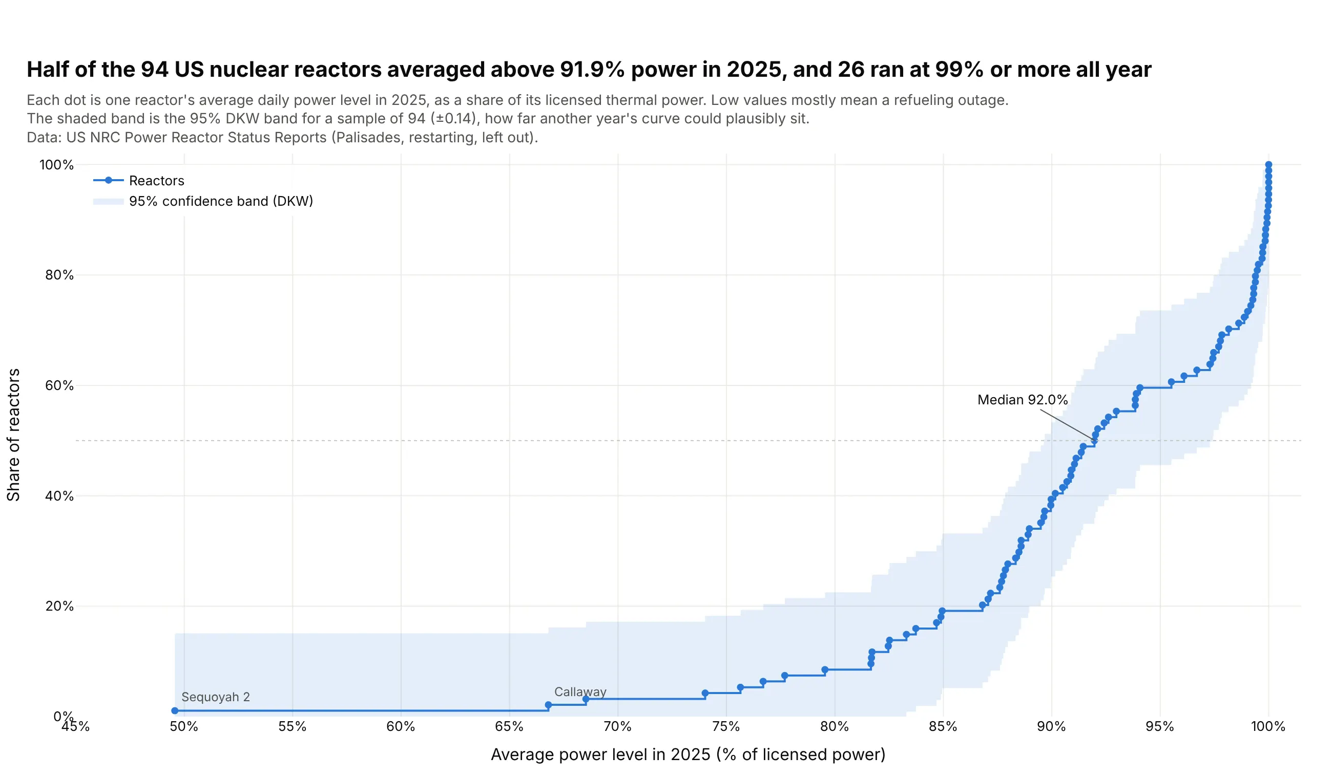
ECDF of the 2025 average power level of 94 US nuclear reactors with a dot for each reactor and a shaded 95% DKW band. The median is 92.0%, 26 reactors averaged 99% or more, and Sequoyah 2 (49.6%) and Callaway (66.8%) are the lowest

With 94 reactors, every one gets a dot on the curve. Half averaged above 91.9% of licensed power in 2025 and 26 ran at 99% or more all year, while the low values are mostly refueling outages. Data: US NRC Power Reactor Status Reports, 2025.

Tip: a Dvoretzky-Kiefer-Wolfowitz band (±0.14 for 94 values) drawn with fill="tonexty" shows how much a small sample's curve could move.

Get the data from the US NRC Power Reactor Status Reports, 2025 full-year file (nrc.gov, power reactor status reports)
and shape it into a table
(columns: date, unit, power = percent of licensed thermal power that morning).

Build a plotly ECDF of each reactor's average power over 2025 (leave out Palisades, which was
being prepared for restart).
- Markers plus a step line, one dot per reactor.
- A shaded 95% band of +/- sqrt(ln(2/0.05) / (2n)) around the curve, clipped to 0..1.
- Label the two lowest reactors and the median. Title with the median and the number at 99%+.

3. Flashy rivers and dammed rivers

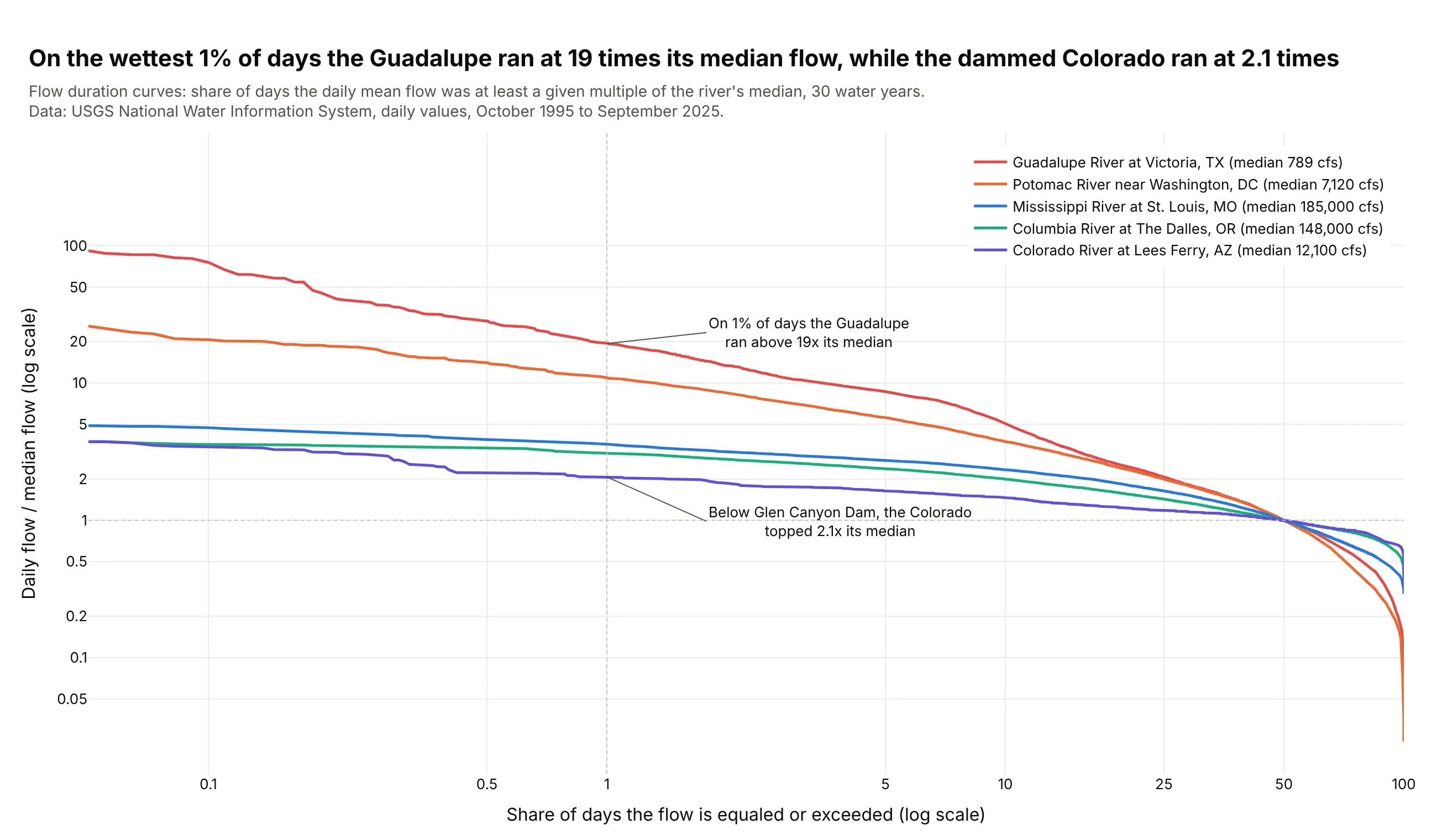
Flow duration curves for five US rivers over 30 years on log axes. On the wettest 1% of days the Guadalupe ran at 19 times its median flow and the Potomac at 11 times, while the Mississippi, the Columbia and the Colorado below Glen Canyon Dam stayed within 2 to 4 times

Hydrologists call this a flow duration curve, a complementary ECDF of daily flow divided by the median. On the wettest 1% of days the Guadalupe ran at 19 times its median flow, while the Colorado below Glen Canyon Dam ran at 2.1 times. Data: USGS National Water Information System, daily values, water years 1996-2025.

Tip: dividing each river by its own median puts a 789 cfs river and a 185,000 cfs river on one axis.

Get the data from USGS National Water Information System daily values (waterservices.usgs.gov), parameter 00060,
for sites 07010000, 14105700, 01646500, 08176500 and 09380000, October 1995 to September 2025,
and shape it into a table
(columns: date, river, cfs = daily mean discharge in cubic feet per second).

Build a plotly flow duration curve: for each river, sort the daily flows from high to low, divide
by the river's median, and plot against the share of days equaled or exceeded.
- Log x axis (0.05% to 100%) and log y axis with "x" tick suffixes; dotted lines at 1x and 1%.
- Label the 1% value for the flashiest and the steadiest river. Legend with each median in cfs.

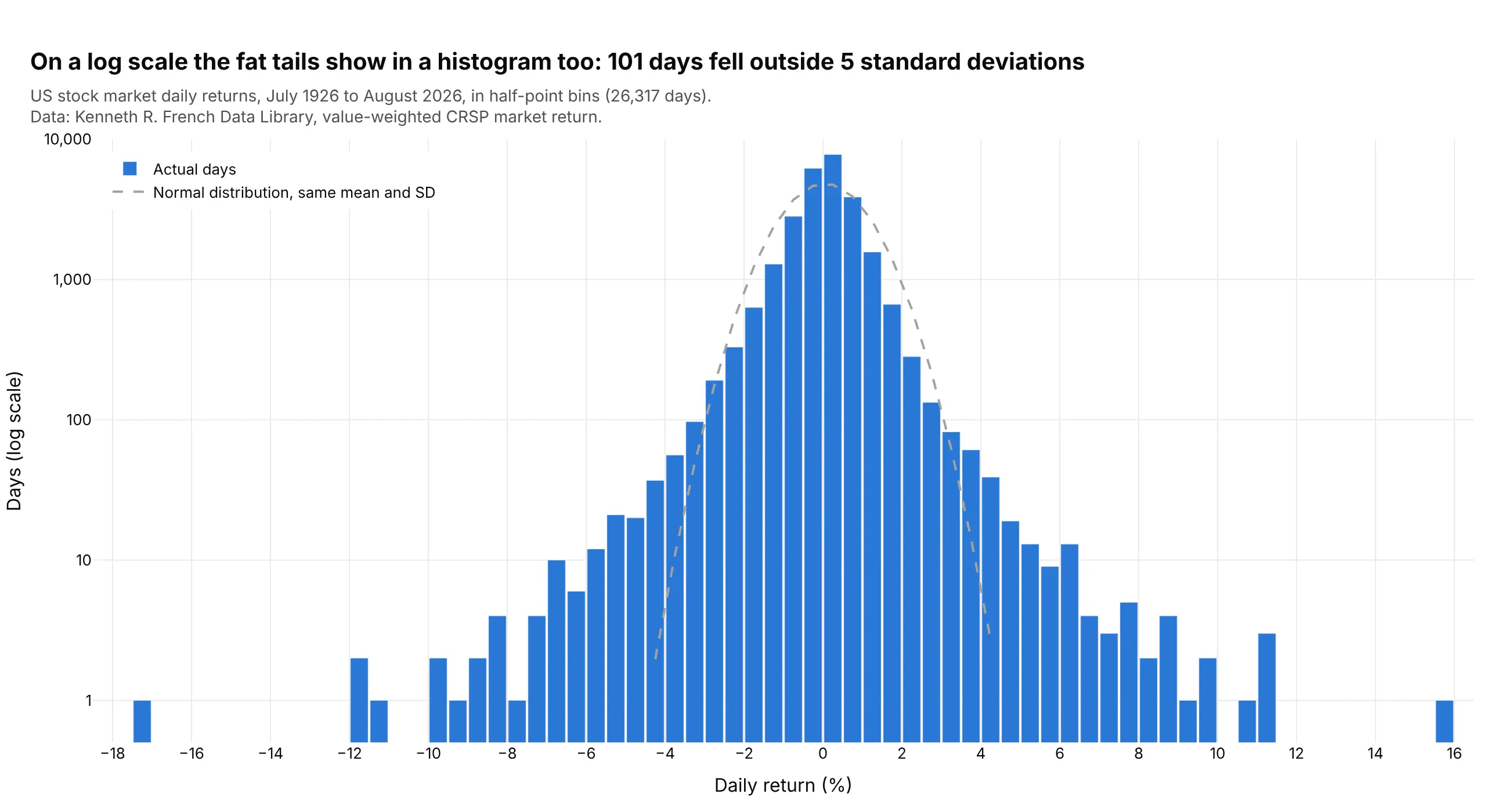
4. A century of stock market days against a normal distribution

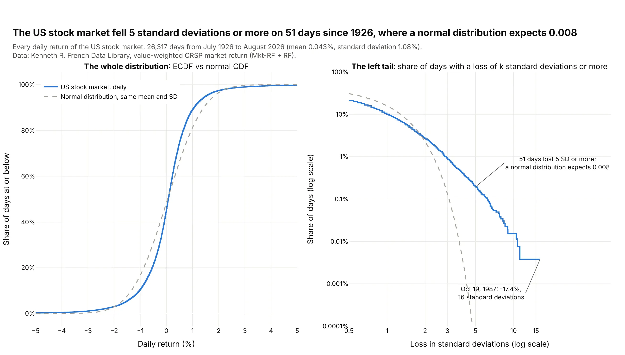
Two panels of US stock market daily returns from 1926 to 2026. Left, the ECDF almost on top of a normal CDF with the same mean and standard deviation. Right, the share of days with losses of k standard deviations or more on log axes: 51 days lost 5 or more where the normal expects 0.008, and October 19, 1987 fell 17.4%, 16 standard deviations

Over 26,317 trading days the ECDF of daily returns looks close to a normal curve, but the log-scale tail on the right tells another story. The market fell 5 standard deviations or more on 51 days, where a normal distribution expects 0.008. Data: Kenneth R. French Data Library, value-weighted CRSP market return, July 1926 to August 2026.

Tip: plot the tail as a complementary ECDF on a log y axis, where a normal curve drops off a cliff and real data doesn't.

Get the data from the Kenneth R. French Data Library, Fama/French 3 Factors [Daily] (mba.tuck.dartmouth.edu)
and shape it into a table
(columns: date, ret = daily market return in percent, Mkt-RF + RF).

Build a plotly figure with two panels.
- Left: the ECDF of ret as a step line and the normal CDF with the same mean and SD dashed, x -5..5.
- Right: for k from 0.5 to 17, the share of days with ret <= mean - k*SD, against the normal tail,
  on log x and log y axes. Label the 5 SD point (actual days vs expected) and the worst day.
- Title with the number of 5 SD losses; print it with the normal expectation to check.

Another way to see it: a histogram on a log y axis shows the same fat tails, with 101 days outside 5 standard deviations either way, but single days scatter as one-day bars.

Histogram of US stock market daily returns from 1926 to 2026 in half-point bins on a log y axis with a dashed normal curve. The normal curve falls below one day beyond about 4% either way, while actual days reach -17.4% and +15.7%

5. Crude oil moves more than Bitcoin on a typical day

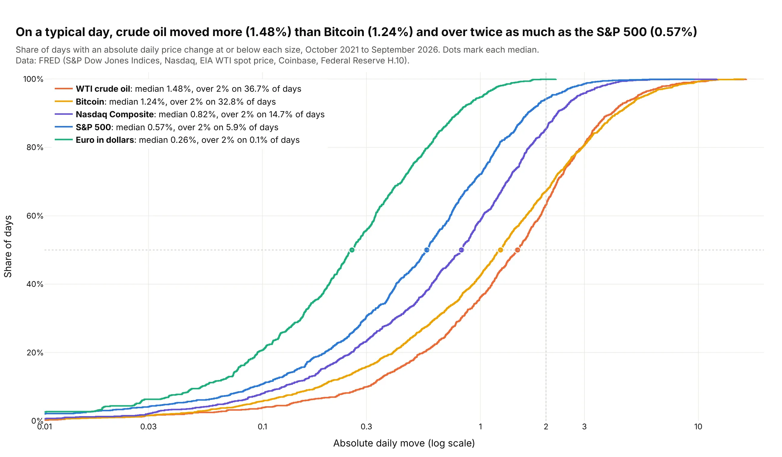
ECDFs of the absolute daily move of five assets from October 2021 to September 2026 on a log axis, with dots at each median: WTI crude oil 1.48%, Bitcoin 1.24%, the Nasdaq Composite 0.82%, the S&P 500 0.57% and the euro in dollars 0.26%

Taking the absolute daily change puts five very different assets on one axis. WTI crude oil's median move was 1.48% over the last five years, more than Bitcoin's 1.24% and over twice the S&P 500's 0.57%. Data: FRED (S&P Dow Jones Indices, Nasdaq, EIA, Coinbase, Federal Reserve H.10).

Tip: put each asset's median and share of days over 2% in the legend, so the key numbers sit next to the curves.

Get the data from FRED (fred.stlouisfed.org): SP500, NASDAQCOM, DCOILWTICO, CBBTCUSD and DEXUSEU,
October 2021 to September 2026,
and shape it into a table
(columns: date, asset, close, move_pct = absolute percent change from the previous close of the same series).

Build a plotly ECDF of move_pct, one step line per asset, on a log x axis from 0.01% to 20%.
- A dot where each curve crosses 50%, and a dotted line at 2%.
- Legend entries "<asset>: median x.xx%, over 2% on y% of days".
- Title with the oil vs Bitcoin comparison; cite FRED and the original publishers.

6. Where Silicon Valley Bank sat among US banks

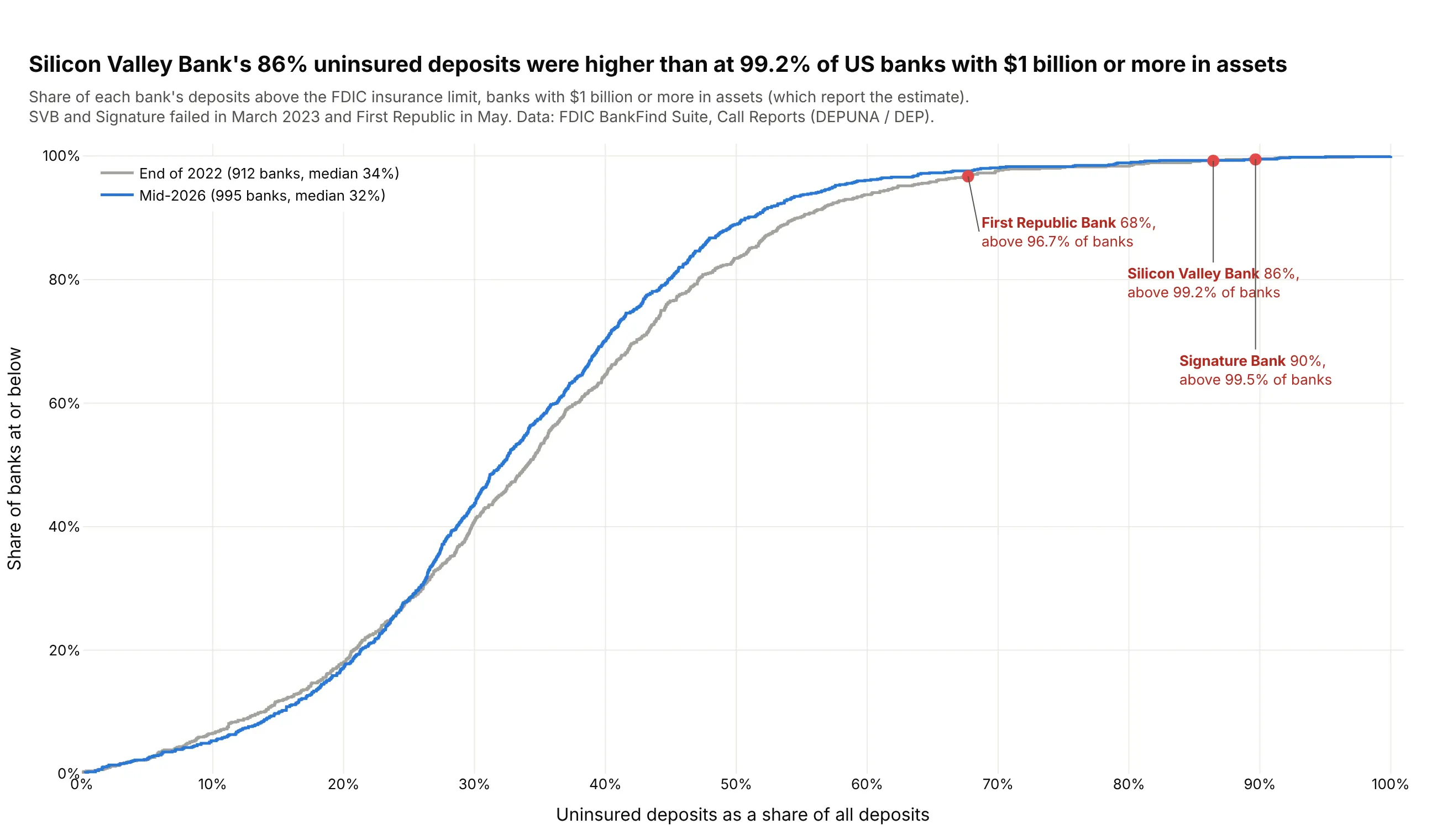
ECDFs of the share of uninsured deposits at US banks with $1 billion or more in assets at the end of 2022 (912 banks, median 34%) and mid-2026 (995 banks, median 32%). Red dots on the 2022 curve mark Silicon Valley Bank (86%, above 99.2% of banks), Signature Bank (90%, above 99.5%) and First Republic Bank (68%, above 96.7%)

The height of an ECDF at any value is a percentile, so marking a bank on the curve shows how unusual it is. At the end of 2022, Silicon Valley Bank's 86% uninsured deposits were higher than at 99.2% of the 912 banks with $1 billion or more in assets. Data: FDIC BankFind Suite, Call Reports for 2022-12-31 and 2026-06-30.

Tip: a single marker on the curve turns the ECDF into a percentile lookup for one company, patient or site.

Get the data from the FDIC BankFind Suite API (api.fdic.gov/banks/financials), report dates 2022-12-31 and 2026-06-30,
fields CERT, NAME, ASSET, DEP, DEPUNA, banks with ASSET >= $1B,
and shape it into a table
(columns: date, cert, name, assets_bn, deposits_bn, uninsured_share = DEPUNA / DEP).

Build a plotly ECDF of uninsured_share, one step line per date (2022 gray, 2026 blue).
- Red dots on the 2022 curve for certs 24735 (SVB), 57053 (Signature) and 59017 (First Republic),
  labeled with their share and the share of banks below them.
- X axis 0-100% with 10% ticks. Title with SVB's percentile; cite the FDIC.

7. How long drug trials take to report results

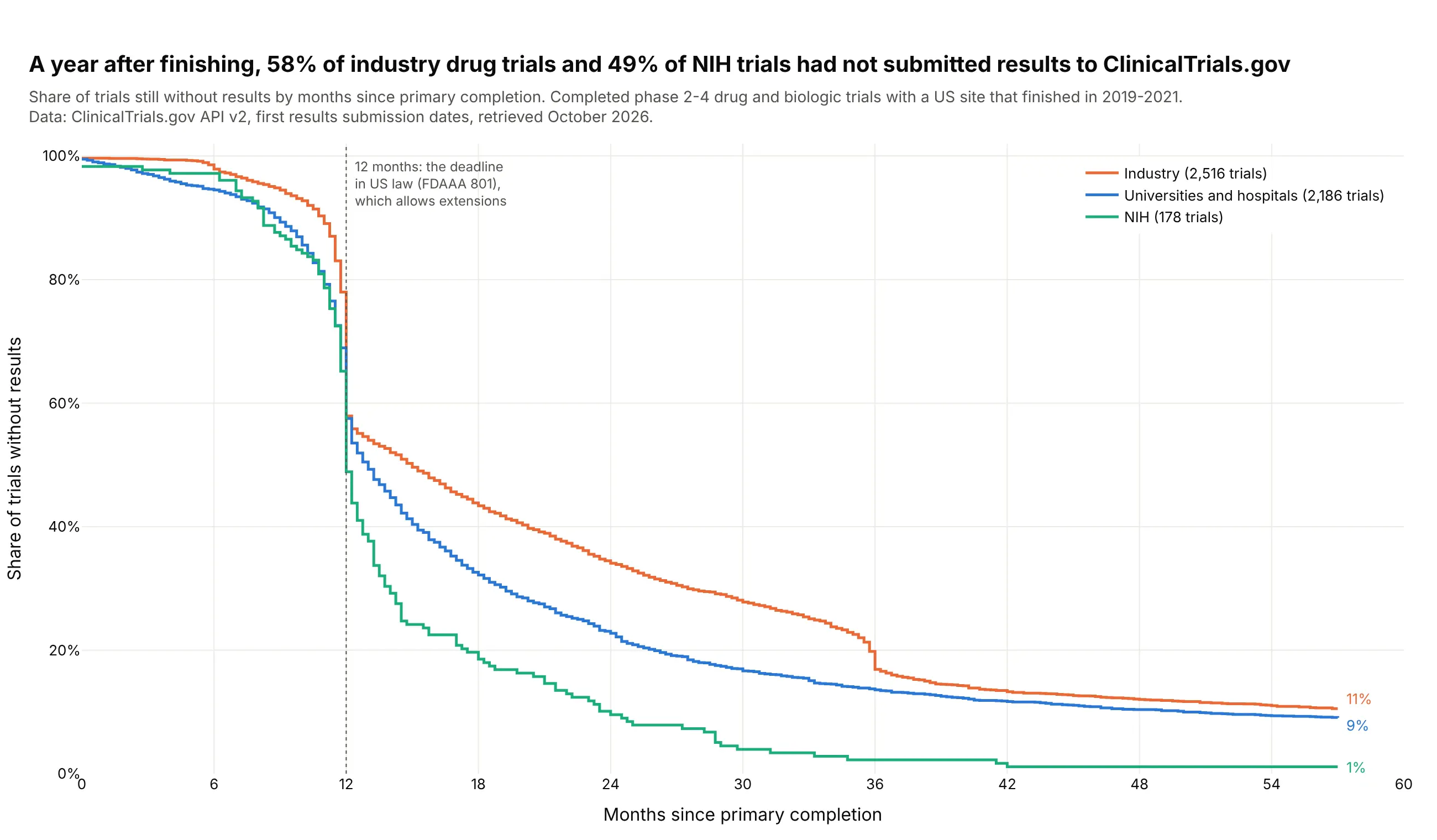
Survival-style curves of the share of completed US drug trials still without results on ClinicalTrials.gov by months since primary completion, for industry (2,516 trials), universities and hospitals (2,186) and NIH (178). At 12 months 58% of industry trials and 49% of NIH trials had not submitted results; after 57 months 11%, 9% and 1% still had none

Drawn as 1 minus the ECDF, results reporting reads like a survival curve. A year after finishing, 58% of the 2,516 industry drug trials and 49% of NIH trials had not submitted results, and 11% of industry trials still had none after 57 months. US law allows some delays beyond 12 months. Data: ClinicalTrials.gov API v2, completed phase 2-4 drug and biologic trials with a US site that finished in 2019-2021.

Tip: keep the trials that never reported in the denominator, so the curves level off above zero instead of pretending everyone reports eventually.

Get the data from the ClinicalTrials.gov API v2 (clinicaltrials.gov/api/v2/studies): completed, interventional,
phase 2-4 drug or biologic trials with a US location and a primary completion date in 2019-2021,
and shape it into a table
(columns: nct_id, sponsor_class, phase, primary_completion, results_submitted, months between them).

Build a plotly step chart of the share of trials still without results against months since
primary completion (0-57), one line per sponsor class: INDUSTRY, OTHER, NIH.
- Trials with no results count as still waiting. Clip negative months to 0.
- A dotted line at 12 months with a note on the FDAAA 801 deadline. Label each line's end value.
- Title with the industry and NIH shares at 12 months.

8. Fine particle pollution days in six US cities

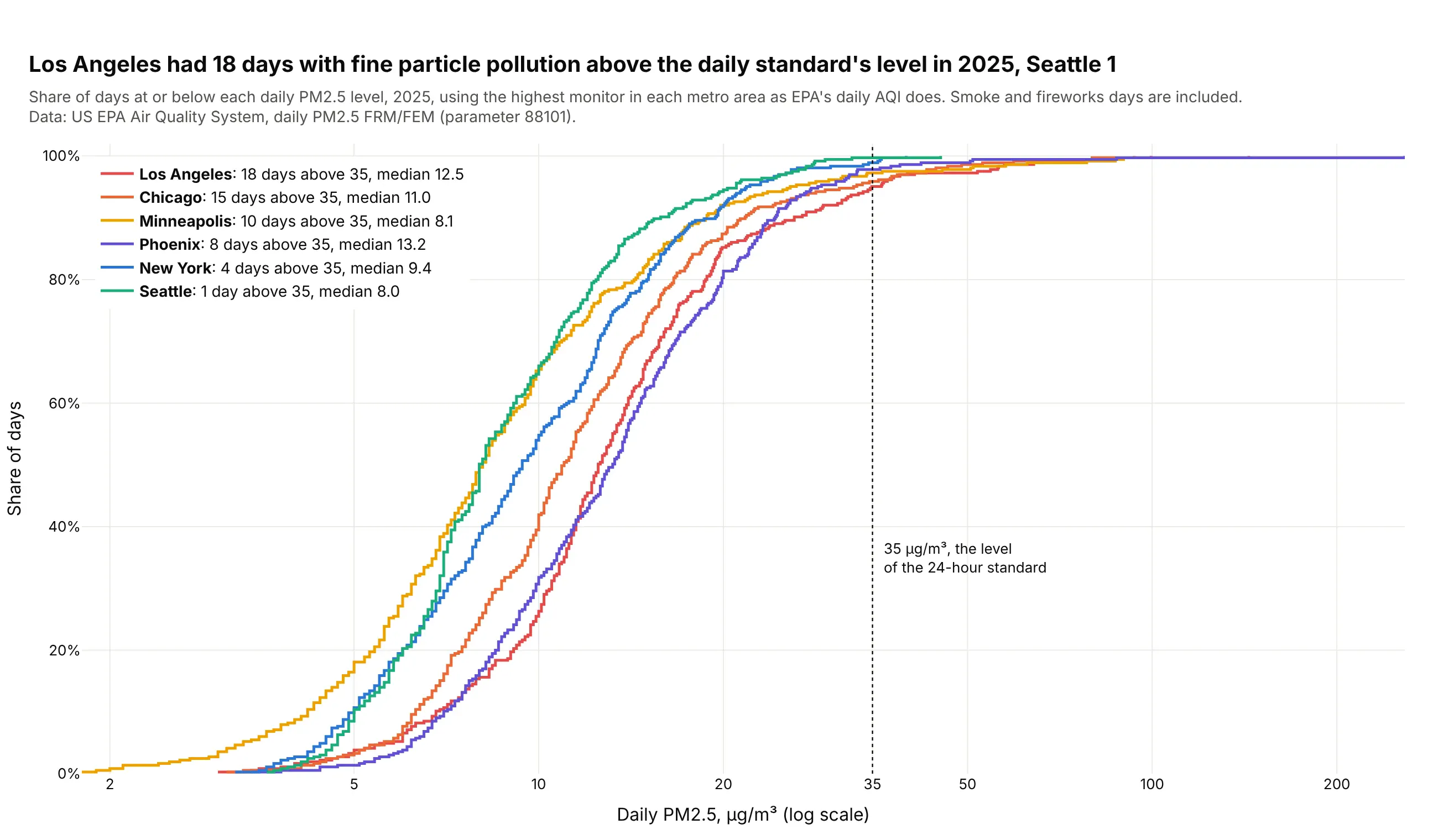
ECDFs of daily PM2.5 in 2025 for six US metro areas on a log axis with a dotted line at 35 micrograms per cubic meter. Days above it: Los Angeles 18, Chicago 15, Minneapolis 10, Phoenix 8, New York 4 and Seattle 1

A threshold line turns an ECDF into a count of bad days: the gap between each curve and 100% at 35 µg/m³ is the share of days above the daily standard's level. Los Angeles had 18 such days in 2025 and Seattle 1. Data: US EPA Air Quality System, daily PM2.5, highest monitor in each metro area.

Tip: a vertical reference line at a regulatory or contractual limit is the most useful line you can add to an ECDF.

Get the data from the US EPA Air Quality System pre-generated daily files (aqs.epa.gov/aqsweb/airdata), PM2.5 88101, 2025,
and shape it into a table
(columns: date, metro, pm25 = highest 24-hour average across the metro's monitors that day, monitors).

Build a plotly ECDF of pm25, one step line per metro, on a log x axis.
- A dotted vertical line at 35 ug/m3 labeled as the level of the 24-hour standard.
- Legend entries "<metro>: N days above 35, median x.x".
- Title with the most and fewest days above 35; say in the subtitle that the highest monitor is used.

9. The Gutenberg-Richter law in 26 years of earthquakes

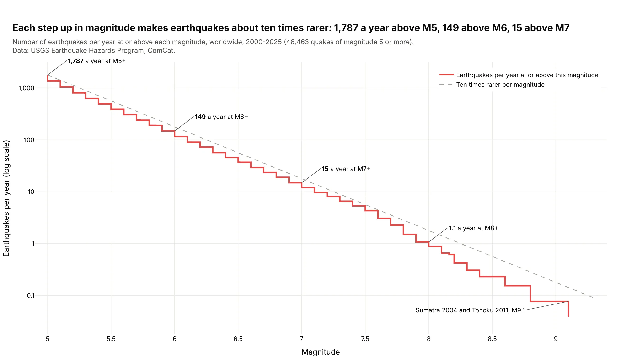
The number of earthquakes per year at or above each magnitude from 2000 to 2025 on a log y axis, falling in a nearly straight line next to a dashed line that drops tenfold per magnitude: 1,787 a year at M5+, 149 at M6+, 15 at M7+ and 1.1 at M8+, ending at the Sumatra 2004 and Tohoku 2011 M9.1 quakes

An unnormalized, reversed ECDF divided by the number of years is the curve seismologists use. Worldwide there were 1,787 earthquakes a year of magnitude 5 or more, 149 of 6 or more and 15 of 7 or more, about ten times fewer per step. Data: USGS Earthquake Hazards Program, ComCat, 2000-2025.

Tip: ecdfnorm=None with ecdfmode="reversed" gives counts at or above each value, and a log y axis turns a power law into a straight line.

Get the data from the USGS ComCat FDSN event service (earthquake.usgs.gov/fdsnws/event/1), minmagnitude 5,
2000-2025, one request per year,
and shape it into a table
(columns: time, mag, depth_km, place).

Build a plotly step chart of earthquakes per year at or above each magnitude (count / 26 years)
on a log y axis, with a dashed reference line that falls tenfold per magnitude from the M5 count.
- Label the counts at M5, M6, M7 and M8 and the two M9.1 quakes.
- Title with the three counts.

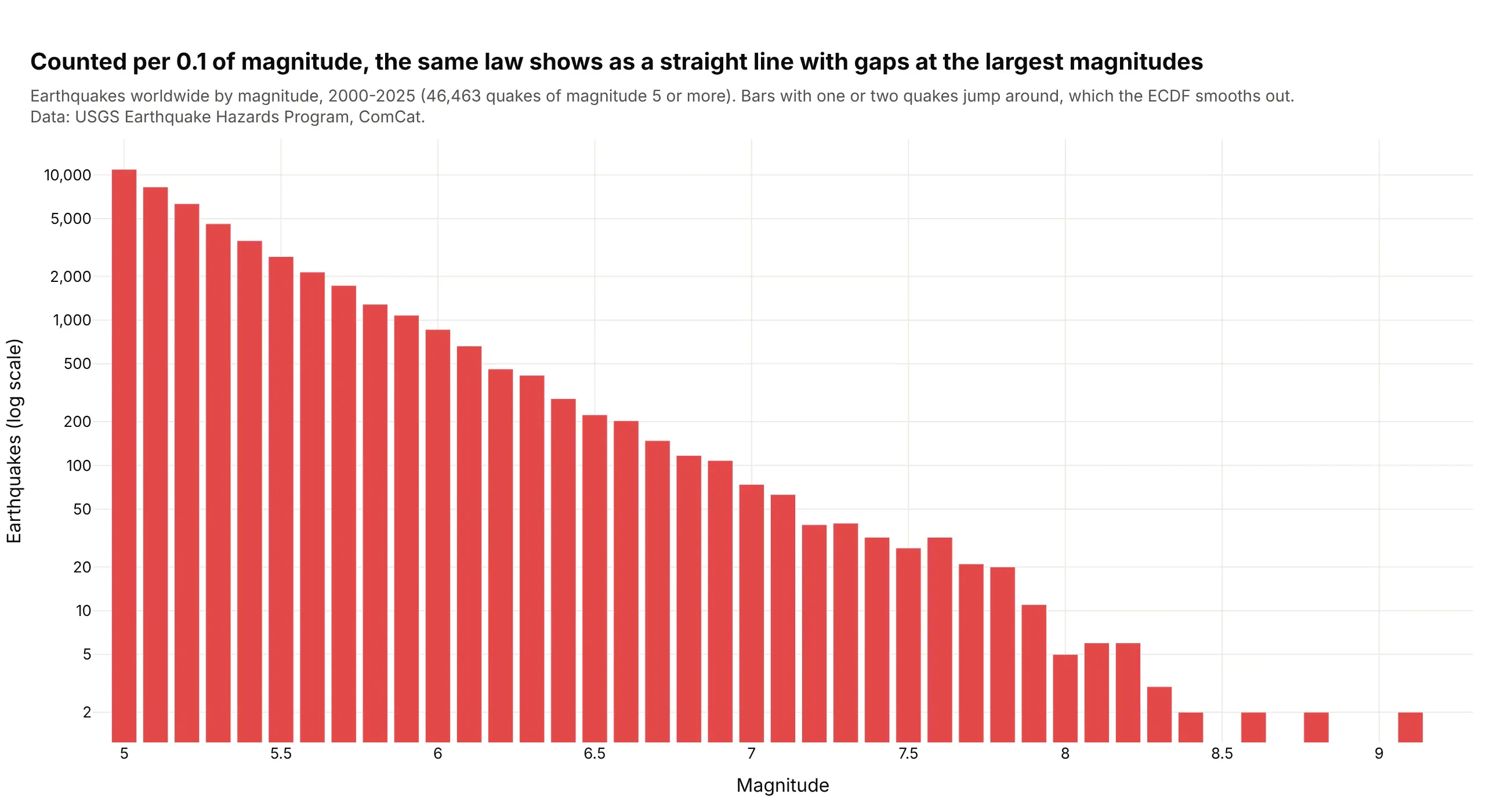
Another way to see it: a histogram of magnitudes in 0.1 steps shows the same straight line on a log axis, but the top bins hold one or two quakes each and jump around.

Histogram of 46,463 earthquakes by magnitude in 0.1 steps from 2000 to 2025 on a log y axis, falling from 10,910 at M5.0 to single digits above M8, with some empty bins above M8.4

10. The 20% tip in New York taxis

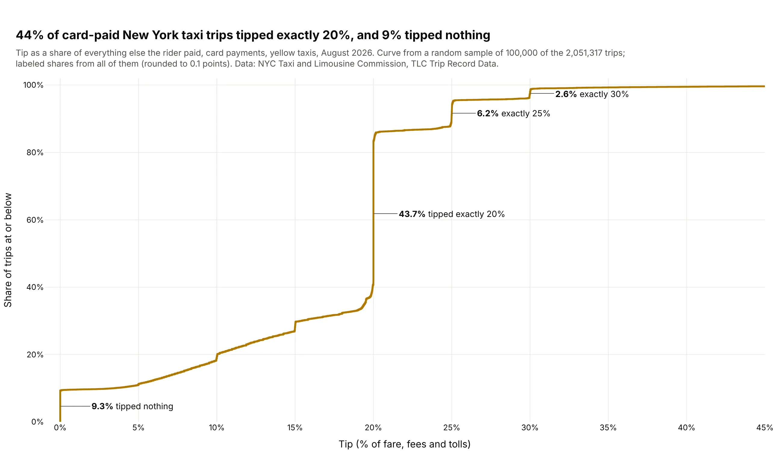
ECDF of tips as a percent of the fare for card-paid New York yellow taxi trips in August 2026, with vertical jumps labeled: 9.3% tipped nothing, 43.7% tipped exactly 20%, 6.2% exactly 25% and 2.6% exactly 30%

A value many people share shows up as a vertical jump in an ECDF, and the height of the jump is its share. 44% of the 2.05 million card-paid yellow taxi trips in August 2026 tipped exactly 20%, and 9% tipped nothing. Data: NYC Taxi and Limousine Commission, TLC Trip Record Data (curve from a sample of 100,000 trips).

Tip: label each jump with its height computed from the full data, since a sample only approximates it.

Get the data from the NYC TLC Trip Record Data, yellow taxi trips, August 2026 (nyc.gov/site/tlc/about/tlc-trip-record-data.page)
and shape it into a table
(columns: tip_pct = tip_amount / (total_amount - tip_amount) x 100, card payments only).

Build a plotly ECDF of tip_pct from 0% to 45% from a random sample of 100,000 trips (seed 0).
- Label the jumps at 0%, 20%, 25% and 30% with their share of all trips (rounded to 0.1 points).
- Title with the 20% and 0% shares; say in the subtitle that the curve is a sample.