Chris Parmer

November 7, 2026

Swimmer Plots - A Complete Guide

TL;DR

A swimmer plot draws one horizontal bar per patient for the time on treatment, sorted by length, with markers along each bar for events such as the start of a response or progression, and an arrow at the end of the bars of patients who are still on treatment.
Swimmer plots are also known as swimmers plots and swim lane plots, and are similar to Gantt charts and sorted bar charts. In cancer trials they sit next to the Kaplan-Meier curve, the tumor waterfall plot, and the spider plot.
Oncologists use them in early-phase trials to see each patient’s story: how fast a response came, how long it lasted, and whether it is still going. Responses are usually graded by RECIST (Response Evaluation Criteria in Solid Tumors), explained below in plain words.
You can make a swimmer plot with Plotly from a go.Bar trace with orientation="h" and go.Scatter marker traces on top. A short helper function is below.

What is a swimmer plot?

Swimmer plots look like this:

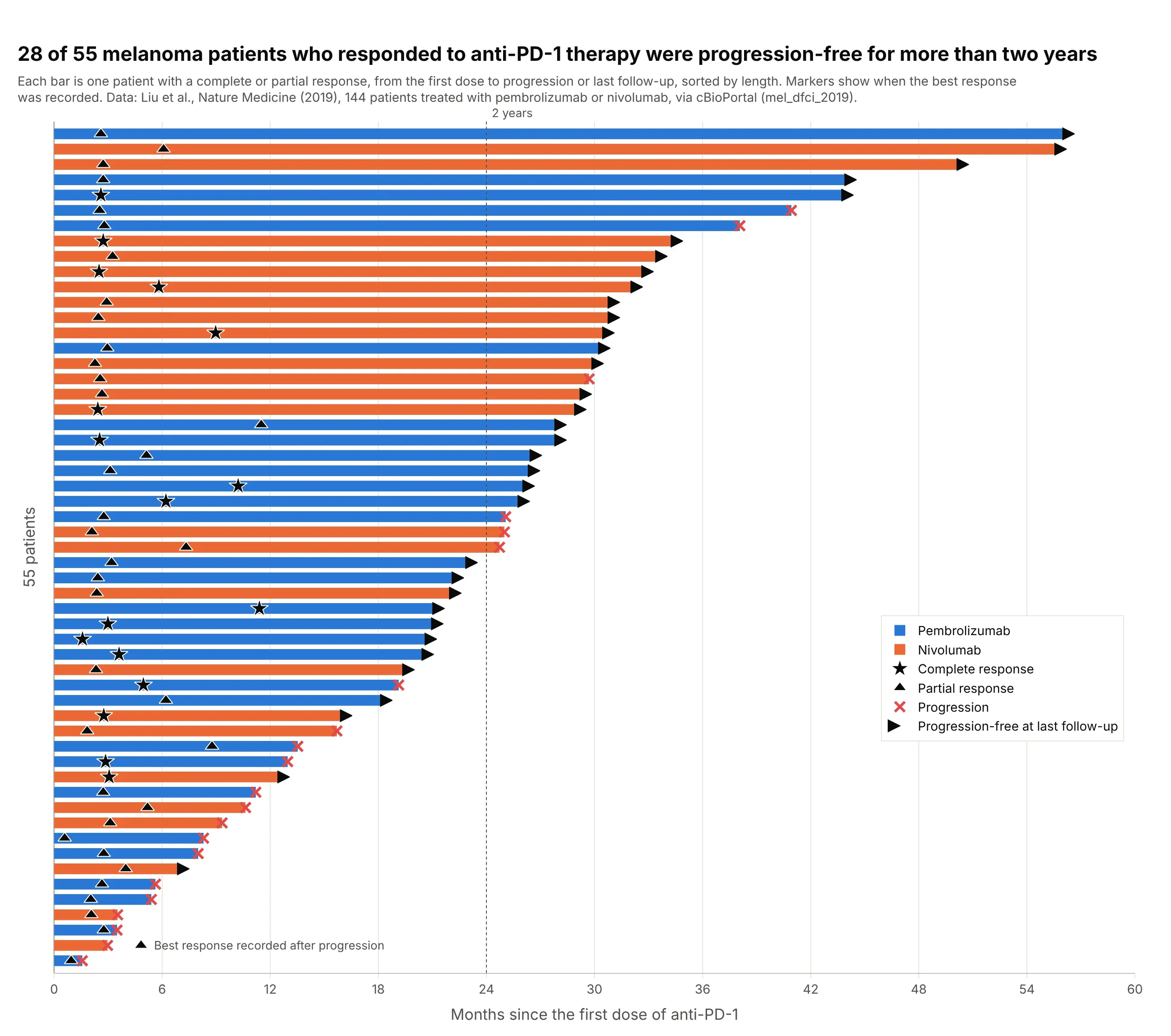
Swimmer plot of 55 melanoma patients who responded to anti-PD-1 therapy: one horizontal bar per patient sorted by length, blue for pembrolizumab and orange for nivolumab, black stars and triangles near 2 to 3 months for complete and partial responses, red crosses at progression on 21 bars, black arrows on 34 bars still progression-free, and a dotted line at 2 years that 28 bars pass

Data: Liu et al. (2019), Nature Medicine, 144 people with metastatic melanoma treated with anti-PD-1 (programmed cell death protein 1) antibodies, via cBioPortal.

How do you read a swimmer plot? In the example above, notice these things:

Each bar is one of the 55 patients whose tumors shrank by a complete or partial response, from the first dose to progression or the last scan. The bars are sorted by length, so the longest stories sit at the top.
The stars (complete response) and triangles (partial response) mark when the best response was recorded. Most sit between two and three months (the median is 2.8 months), around the time of the first scans, and a few best responses came later, up to 11.5 months.
A red cross means the cancer progressed; an arrow means the patient was still progression-free at the last follow-up. Of the 55 bars, 34 end in an arrow, so their bars are still growing.
Twenty-eight of the 55 responders passed the dotted two-year line, and the longest was progression-free for about 56 months. The color of each bar shows the drug, and both drugs reach the top.

It’s often used for charts like these:

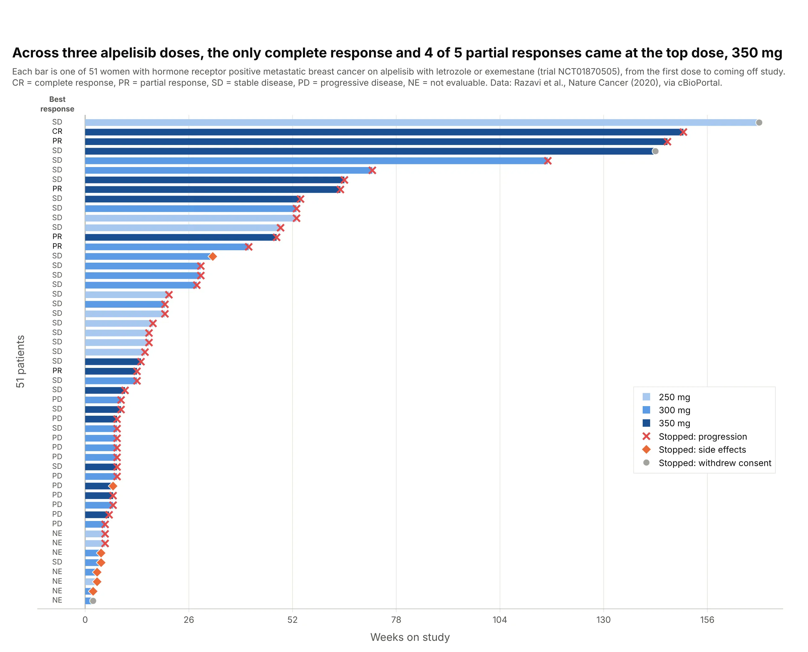
Swimmer plot of 51 women in a phase I/II alpelisib trial, bars in three blues for 250, 300, and 350 mg, sorted by weeks on study, with a column of best response letters at the left and red crosses, orange diamonds, or gray dots at the end of each bar for progression, side effects, or withdrawn consent; the only CR and four of five PRs are in the darkest blue

Dose-finding trials. In a phase I/II trial of alpelisib plus letrozole or exemestane at three daily doses, the only complete response and four of the five partial responses came at the highest dose, 350 mg, which coloring the bars by dose shows at a glance. Data: Razavi et al. (2020), Nature Cancer, via cBioPortal.

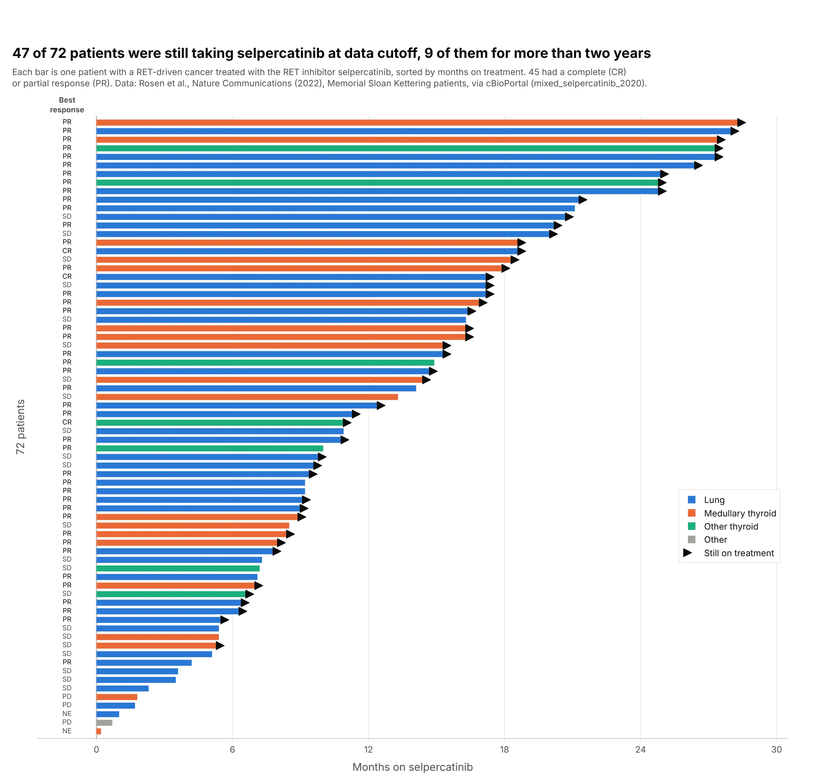
Swimmer plot of 72 patients treated with selpercatinib, bars colored by lung, medullary thyroid, other thyroid, and other cancers, sorted by months on treatment up to 28.3, best response letters at the left, and arrows on the 47 patients still on treatment

Targeted therapy across tumor types. Forty-seven of 72 patients with RET-driven lung and thyroid cancers (cancers driven by a change in the RET gene) were still taking the RET inhibitor selpercatinib at data cutoff, nine of them for more than two years. Data: Rosen et al. (2022), Nature Communications, via cBioPortal.

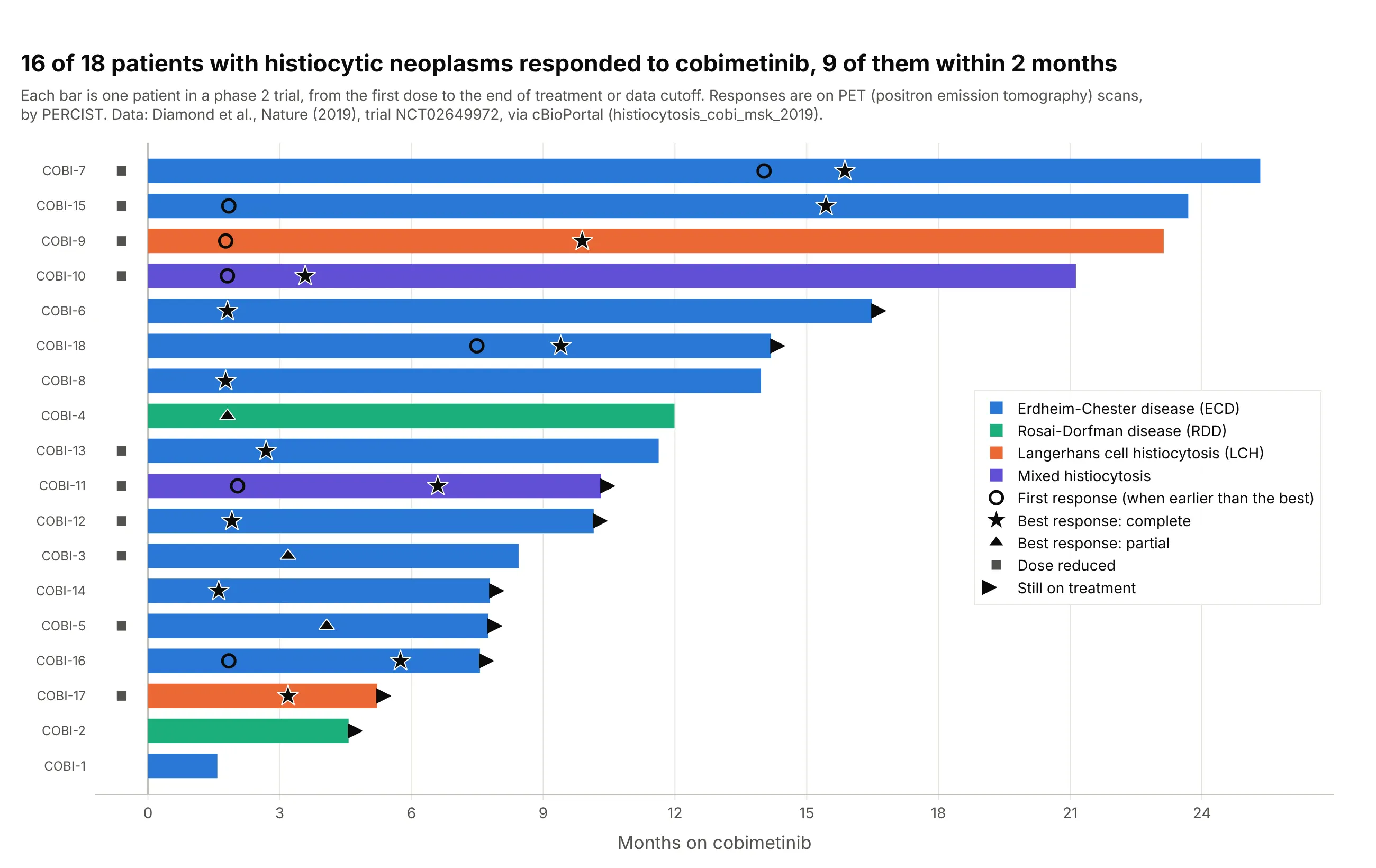
Swimmer plot of 18 patients with histiocytic neoplasms on cobimetinib, labeled COBI-1 to COBI-18, bars colored by disease, open circles at the first response, stars and triangles at the best complete or partial response, gray squares for dose reductions, and arrows on the nine still on treatment

Small trials in rare diseases. Sixteen of 18 patients with histiocytic neoplasms, rare disorders of immune cells called histiocytes, responded to cobimetinib, a drug that blocks the MEK protein in a cell-growth signaling pathway, on PET (positron emission tomography) scans, nine of them within two months, and for seven the response kept deepening after the first scan. Data: Diamond et al. (2019), Nature, trial NCT02649972, via cBioPortal.

A short history

The earliest how-to for the chart that we found comes from the clinical programming community: at PharmaSUG 2014, the pharmaceutical industry’s SAS users’ conference, Stacey Phillips presented “Swimmer Plot: Tell a Graphical Story of Your Time to Response Data Using PROC SGPLOT” (Phillips 2014), and SAS’s Sanjay Matange followed with a swimmer plot post the same June. Phillips’s paper already had every convention in use today: bars for treatment duration colored by a baseline group, triangles where a complete or partial response starts, a dot where it ends, and an arrow for a response that continues. Here is the paper’s own example, redrawn:

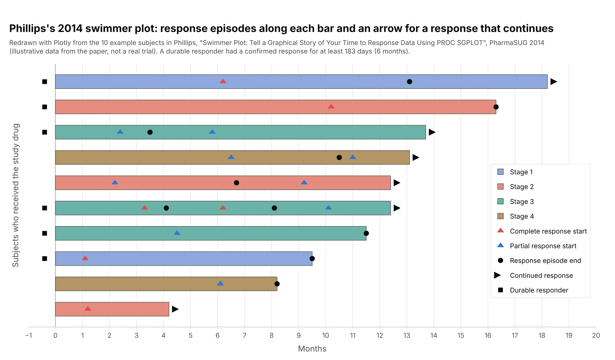
Redraw of the Phillips 2014 swimmer plot: 10 bars colored by disease stage 1 to 4, red and blue triangles where complete and partial responses start, black dots where response episodes end, arrows on six bars for continued responses, and black squares at the left for durable responders

Data: the 10 example subjects printed in Phillips (2014), illustrative data from the paper, not a real trial.

How tumor response is measured: RECIST in plain words

Most swimmer plots in oncology mark responses graded by RECIST, the Response Evaluation Criteria in Solid Tumors. RECIST 1.0 came out in 2000 (Therasse et al. 2000) and the current version, 1.1, in 2009 (Eisenhauer et al. 2009). It turns CT (computed tomography) or MRI (magnetic resonance imaging) scans into a few categories that every trial reports the same way.

At the start of treatment, a radiologist picks up to five measurable tumors, the target lesions, with at most two per organ, measures the longest diameter of each, and adds them up. Every later scan is compared with that sum (RECIST working group of the European Organisation for Research and Treatment of Cancer, EORTC):

Complete response (CR): every target lesion has disappeared (lymph nodes count as normal again below 10 mm across).
Partial response (PR): the sum has shrunk by 30% or more from the start.
Progressive disease (PD): the sum has grown by 20% or more from its smallest value on study, and by at least 5 mm, or a new tumor has appeared.
Stable disease (SD): neither of the above.

A patient’s best overall response is the best category over all scans, and in single-arm trials a complete or partial response counts only when a scan at least four weeks later confirms it. Here are the 69 selpercatinib patients with a measured best change, placed in the RECIST zones:

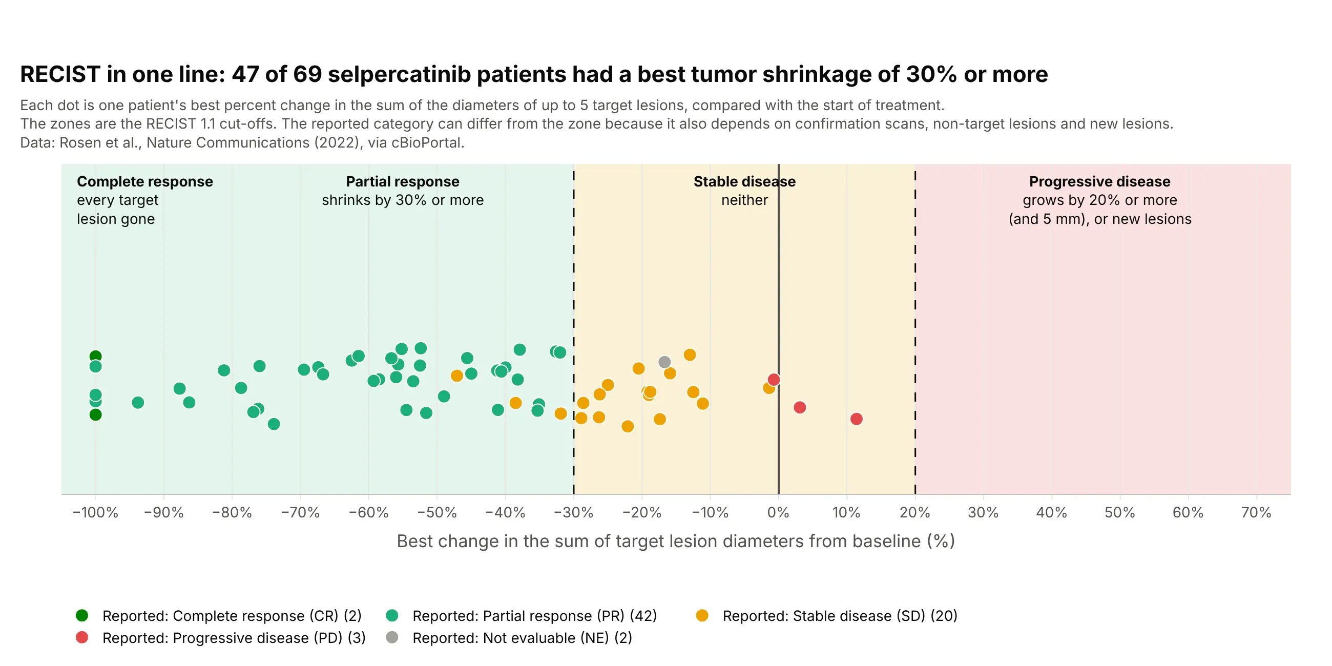
Dot plot of the best percent change in tumor size for 69 selpercatinib patients across shaded RECIST zones: complete response at minus 100%, partial response from minus 30% down, stable disease between minus 30% and plus 20%, progressive disease above plus 20%; 47 dots are at minus 30% or lower, colored by the response each patient was reported with

Data: Rosen et al. (2022), Nature Communications, via cBioPortal.

A few dots sit in a different zone from the category they were reported with, because the category also depends on confirmation scans, on the non-target lesions that are followed but not measured, and on new lesions. On a swimmer plot, the response marker goes at the date of the scan that first showed the response, and the progression marker at the scan that showed progression. Blood cancers, brain tumors, and PET-based trials use their own criteria (the Lugano classification, RANO for Response Assessment in Neuro-Oncology, and PERCIST for PET Response Criteria in Solid Tumors), but the swimmer plot draws them the same way.

Alternatives to a swimmer plot

Here’s the same selpercatinib data drawn six ways. Some are better for the question, some worse, some just different:

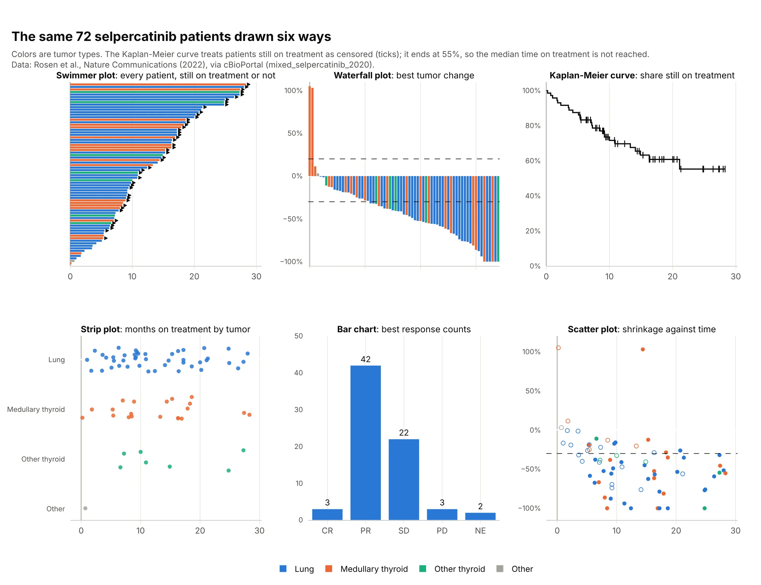
The 72 selpercatinib patients drawn six ways: a swimmer plot with arrows, a waterfall plot of the best tumor change from plus 105% to minus 100%, a Kaplan-Meier curve of the share still on treatment that ends at 55%, a strip plot of months on treatment by tumor type, a bar chart of best response counts with 42 partial responses, and a scatter plot of best change against months on treatment

Swimmer plot (best for individual stories). It is the only one of the six that shows, for each patient, how long treatment lasted and whether it is still going.
Tumor waterfall plot (different). One bar per patient for the best percent change in tumor size, sorted from growth to shrinkage, answers “how deep” where the swimmer plot answers “how long”. Trial reports usually show both, often side by side with the patients in the same order. It shares a name with the financial waterfall chart but not the logic.
Kaplan-Meier curve (better for comparing groups). It handles the 47 patients still on treatment properly as censored and gives a curve you can compare between arms, which here stays above 55%, so the median time on treatment is not reached. It hides who the patients are.
Strip plot of durations (worse). The dots show the spread by tumor type, but they can’t show which patients are still on treatment, so short follow-up looks like short benefit.
Bar chart of best responses (worse). Forty-two partial responses is the headline number for a response rate, but it drops time entirely.
Scatter plot of shrinkage against time (works too). It asks whether deeper responses last longer, which the swimmer plot can only hint at.

The tumor waterfall plot is the swimmer plot’s usual companion in trial reports, so here it is on its own, on the same 69 patients as the RECIST figure above:

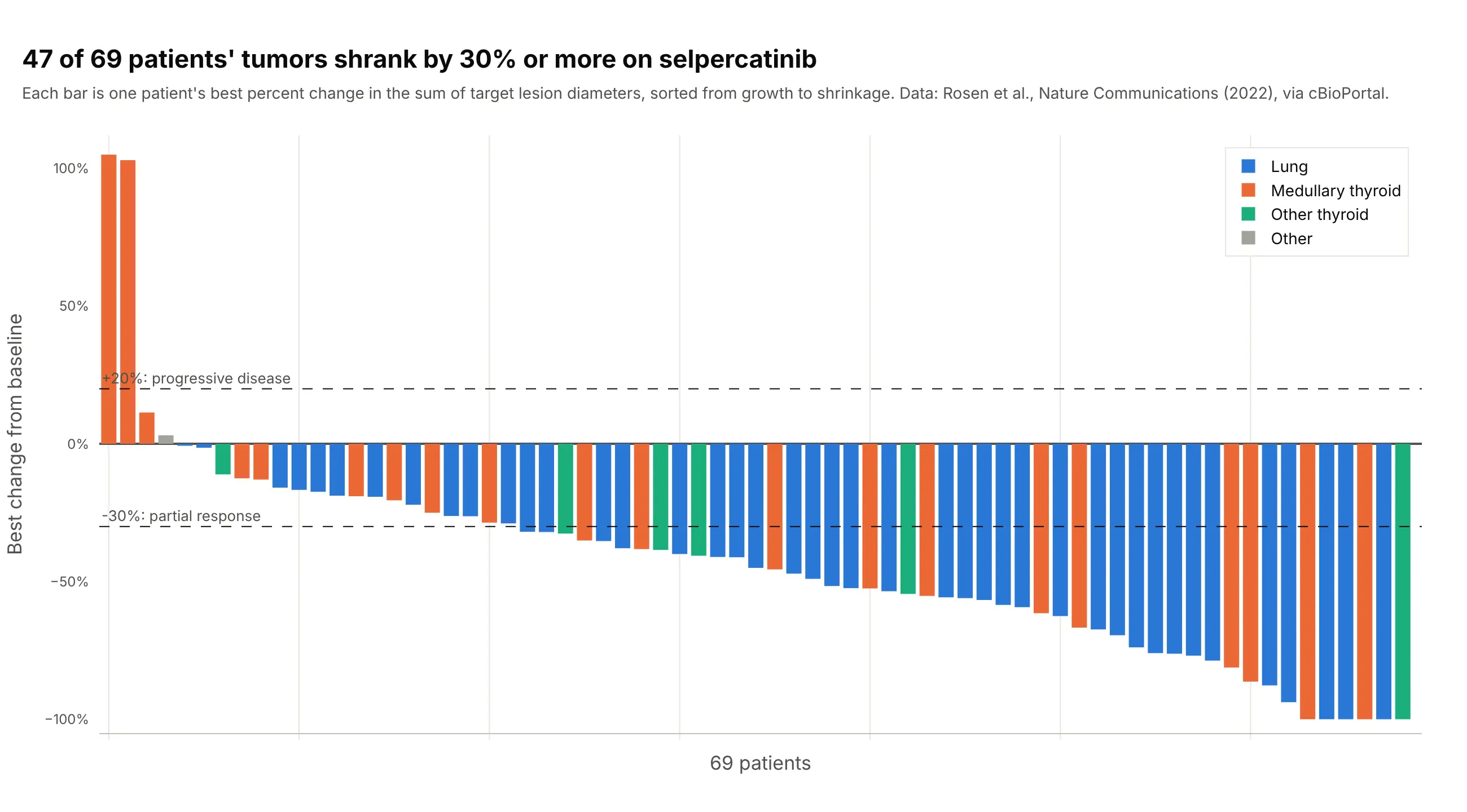
Tumor waterfall plot of 69 selpercatinib patients: one bar per patient for the best percent change in tumor size, sorted from about plus 105% to minus 100%, colored by tumor type, with dashed lines at plus 20% and minus 30%; 47 bars reach minus 30% or lower

Data: Rosen et al. (2022), Nature Communications, via cBioPortal.

A spider plot is the other close relative: one line per patient for the percent change in tumor size at every scan, which needs scan-by-scan measurements that most public datasets don’t include. A Gantt chart is the version on a calendar axis, with each bar starting on its own date; a swimmer plot starts every bar at zero so durations can be compared. A forest plot summarizes the same trial as effect sizes by subgroup.

How to make a swimmer plot

With AI

ChatGPT, Claude Code, GitHub Copilot, Cursor, and other AI tools are excellent at writing Plotly code. Name Plotly in the prompt, and say what the bars, the markers, and the arrows mean:

Make a plotly swimmer plot from cobimetinib.csv (columns: patient, disease, months_on_treatment, on_treatment,
months_to_first_response, months_to_best_response, pet_best_response, dose_reduction).

- One horizontal go.Bar per patient (orientation="h"), sorted by months_on_treatment, longest at the top, colored by disease.
- go.Scatter markers on the bars: an open circle at the first response, a star at a complete best response,
  a triangle at a partial one.
- An arrow-right marker just past the end of the bar for patients with on_treatment = 1.
- A legend that explains every color and marker, and patient labels on the y axis.
- Check: print how many patients are still on treatment and how many responded.

With Plotly Studio

Plotly Studio is a desktop app where you point an AI at a dataset and it builds charts and a Dash app around your questions. Ask for a swimmer plot the same way:

Show a swimmer plot of months on treatment for each patient, sorted by length and colored by dose level, with a star at the first response, a red cross at progression, an arrow for patients still on treatment, and a dropdown to pick the cohort.

Make a swimmer plot in Python or JavaScript

This is the code AI tools write under the hood. Plotly has no dedicated swimmer plot trace, so a swimmer plot is a go.Bar trace with orientation="h", one bar per patient, plus go.Scatter traces for the event markers and the arrows. This helper returns a go.Figure, and every example in this guide builds on the same idea:

import pandas as pd
import plotly.graph_objects as go


def swimmer(df, length, color=None, events=None, ongoing=None):
    """A swimmer plot in Plotly: one sorted horizontal bar per patient, event markers and arrows for ongoing ones."""
    df = df.sort_values(length).reset_index(drop=True)
    y = df.index
    fig = go.Figure()
    for key, g in df.groupby(color) if color else [("", df)]:
        fig.add_trace(go.Bar(x=g[length], y=g.index, orientation="h", width=0.7, name=str(key)))
    for name, (col, symbol) in (events or {}).items():
        fig.add_trace(go.Scatter(x=df[col], y=y, mode="markers", name=name,
                                 marker=dict(symbol=symbol, size=13, color="black", line=dict(color="white", width=1))))
    if ongoing:
        on = df[df[ongoing] == 1]
        fig.add_trace(go.Scatter(x=on[length] + 0.3, y=on.index, mode="markers", name="Still on treatment",
                                 marker=dict(symbol="arrow-right", size=13, color="black")))
    fig.update_layout(barmode="overlay", template="simple_white", yaxis_visible=False,
                      xaxis_title="Months on treatment")
    return fig


df = pd.read_csv("cobimetinib.csv")  # patient, disease, months_on_treatment, on_treatment, months_to_first_response, ...
fig = swimmer(df, "months_on_treatment", color="disease", ongoing="on_treatment",
              events={"First response": ("months_to_first_response", "circle-open"),
                      "Best response": ("months_to_best_response", "star")})
fig.show()

The y values are row numbers after sorting, so the bars stay in order however many colors there are, and barmode="overlay" keeps each color’s bars in their own row. For a marker at a time without a date, such as a dose reduction, put it at a small negative x to the left of the bar.

In JavaScript, plotly.js draws the same thing with one bar trace and two scatter traces:

<div id="chart"></div>
<script src="https://cdn.plot.ly/plotly-4.1.1.min.js"></script>
<script>
  // Months on cobimetinib for 18 patients, sorted (Diamond et al., Nature 2019; cBioPortal histiocytosis_cobi_msk_2019)
  const months = [1.58, 4.57, 5.22, 7.56, 7.75, 7.79, 8.44, 10.15, 10.32, 11.63, 11.99, 13.96, 14.19, 16.49, 21.13, 23.13, 23.69, 25.33];
  const best = [null, 1.81, 3.19, 5.75, 4.07, 1.61, 3.19, 1.91, 6.60, 2.69, 1.81, 1.77, 9.40, 1.81, 3.58, 9.89, 15.44, 15.87];
  const ongoing = [0, 1, 1, 1, 1, 1, 0, 1, 1, 0, 0, 0, 1, 1, 0, 0, 0, 0];
  const y = months.map((_, i) => i);
  const on = y.filter(i => ongoing[i]);

  Plotly.newPlot("chart", [
    {type: "bar", orientation: "h", x: months, y: y, width: 0.7, marker: {color: "#2a78d6"}, name: "Months on treatment"},
    {type: "scatter", mode: "markers", x: best, y: y, name: "Best response",
     marker: {symbol: "star", size: 14, color: "black", line: {color: "white", width: 1}}},
    {type: "scatter", mode: "markers", x: on.map(i => months[i] + 0.3), y: on, name: "Still on treatment",
     marker: {symbol: "arrow-right", size: 13, color: "black"}}
  ], {
    width: 900, height: 500, barmode: "overlay",
    xaxis: {title: {text: "Months on cobimetinib"}}, yaxis: {visible: false}
  });
</script>

Share it

Every Plotly chart has a Share chart button (the cloud icon in its toolbar) that uploads it to Plotly Cloud and gives you a link. Only you can see it until you change its visibility.

For a live app, put the chart in a Dash app and publish it with the Plotly Cloud CLI. Coding agents can run these commands for you:

pip install "dash[cloud]"
plotly user login
plotly app publish

If your data has to stay in your own cloud or data center, publish to Dash Enterprise instead.

Dos and don’ts

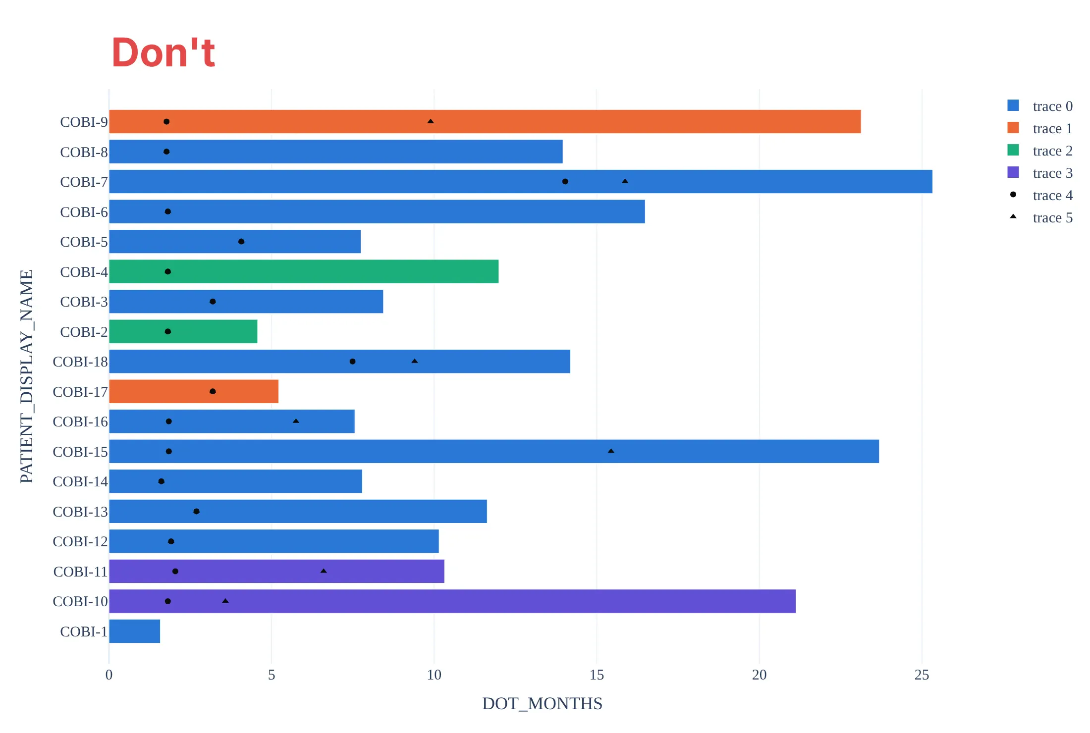
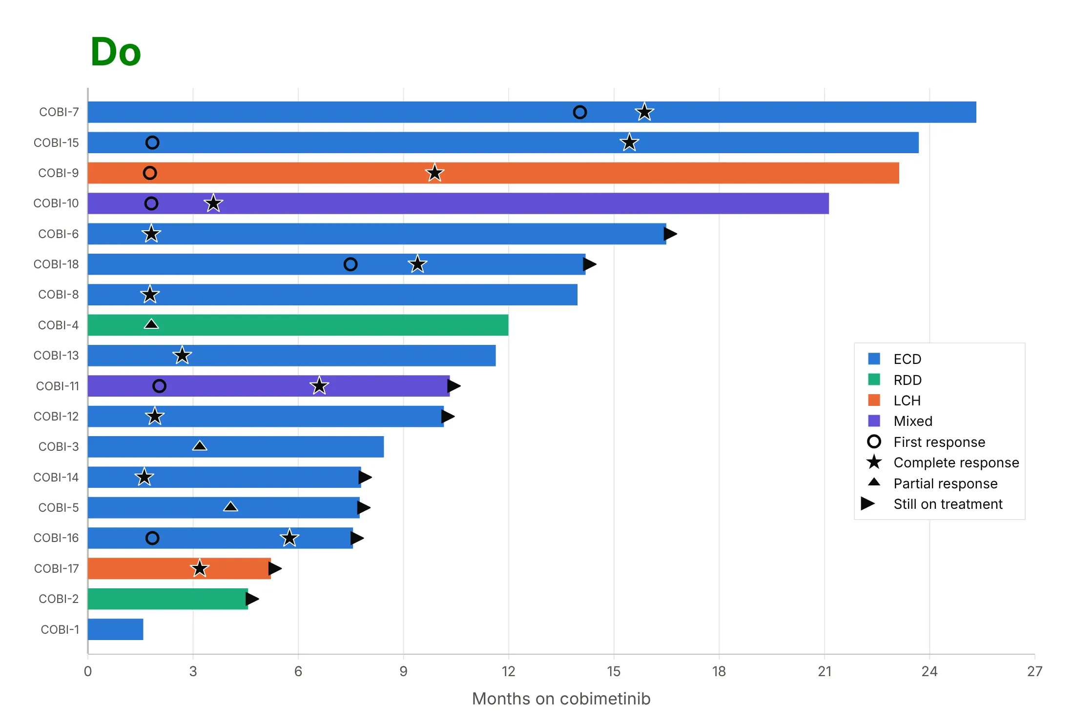
Most of the work in a swimmer plot is the order of the bars and making the markers readable. Here are the 18 cobimetinib patients both ways, in the same colors.

Don’t order the bars by patient ID (here sorted as text, so COBI-10 follows COBI-1), leave out the arrows for patients still on treatment, draw small markers with no outline that sink into the bars and don’t say which response is which, or keep the default legend, raw column names, and a serif font:

The 18 cobimetinib patients in patient ID text order with no arrows, small black dots and triangles without outlines, a legend of trace 0 to trace 5, axis titles DOT_MONTHS and PATIENT_DISPLAY_NAME, and a serif font

Do sort the bars by time on treatment, mark the first and the best response with outlined symbols named in the legend, add an arrow for every patient still on treatment, and label the axis in plain words:

The same patients sorted by months on cobimetinib, with open circles at the first response, outlined stars and triangles at the best complete or partial response, arrows on the nine still on treatment, and a legend that names every color and symbol

Checklist

Sort the bars by time on treatment, or group them first (by dose, arm, or best response) and sort inside each group.
Start every bar at zero (the first dose or randomization), and say in the subtitle what the end of a bar means.
Draw an arrow for every patient still on treatment or still progression-free, and explain it in the legend.
Use outlined black or dark markers for events, so they read on any bar color, and keep red for progression.
Say which response criteria were used (RECIST 1.1, PERCIST, RANO) and where the data cutoff was.

Don’t

Read a short bar with an arrow as a short benefit: it only means the patient started recently.
Show only responders without saying so, since that hides the denominator; example 3 below shows everyone.
Use the swimmer plot to compare arms in a randomized trial; that is what a Kaplan-Meier curve is for.
Put patient names, initials, or dates of birth on the axis; use the study’s anonymous ID or no labels.

Options to customize

A swimmer plot in Plotly is a horizontal bar trace plus scatter traces, so these are the options that matter most. The full lists are in the bar trace reference and the scatter trace reference.

go.Bar(orientation="h", x=..., y=...): one bar per patient; x is the time on treatment, y the patient’s row.
width on the bar trace: the bar thickness in rows (0.6 to 0.8 leaves a gap); set it explicitly when you split the bars into several traces.
barmode="overlay": keeps bars from different color traces in their own rows, and lets a pale bar (planned or licensed time) sit behind a dark one.
base on the bar trace: start bars somewhere other than zero, for a phase that begins later (a maintenance period, a crossover).
marker.symbol on go.Scatter: "star", "triangle-up", "circle-open", "x-thin", "diamond" for events and "arrow-right" for ongoing treatment; see the marker symbols.
marker.line: a white outline around black markers so they stay visible on every bar color.
yaxis.categoryorder="array" with categoryarray, or numeric rows: fix the sort order when y holds patient IDs.
mode="text" on a scatter at a negative x: a column of best response letters or dose levels to the left of the bars.
fig.add_vline(x=24): a reference time such as six months or two years.
hovertemplate with customdata: patient ID, dose, and best response on hover.
make_subplots(cols=3, shared_xaxes=True): one panel per arm or cohort when there are hundreds of patients.

More swimmer plot examples

Six more swimmer plots built from real public data, each with its source, the technique that makes it work, and a prompt to rebuild it. Four are oncology trials; the last three show that the same chart works for anything with a lifetime: nuclear reactors, Mars rovers, and Python releases.

1. A randomized kidney cancer trial: one panel per arm

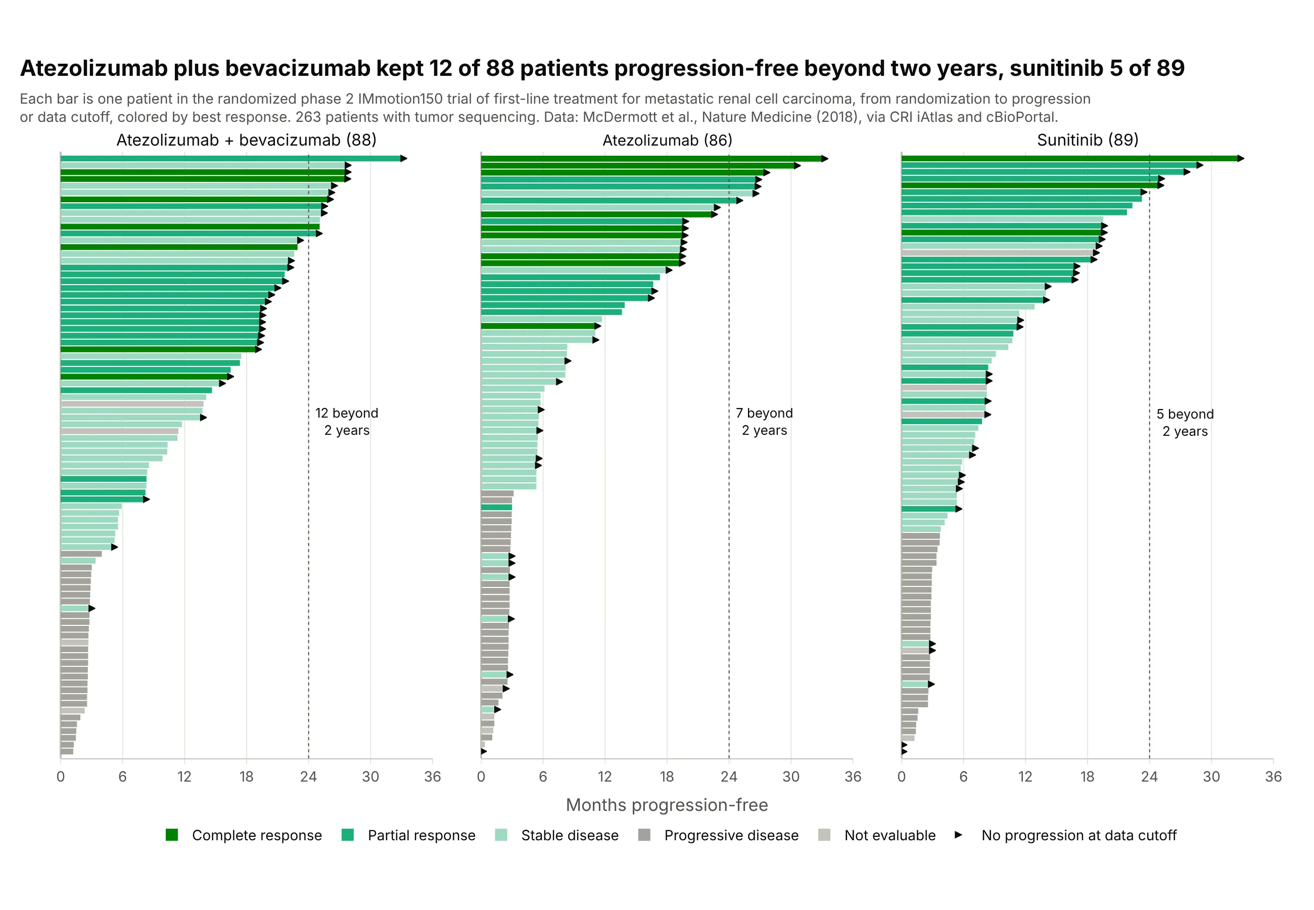
Three swimmer panels for the IMmotion150 arms, atezolizumab plus bevacizumab (88), atezolizumab (86), and sunitinib (89), thin bars sorted by progression-free months and colored by best response from dark green for complete response to gray for progressive disease, small arrows for patients without progression, and labels of 12, seven, and five patients beyond the 2-year line

In the IMmotion150 trial of first-line treatment for metastatic kidney cancer, 12 of 88 patients on atezolizumab plus bevacizumab were progression-free beyond two years, against seven of 86 on atezolizumab alone and five of 89 on sunitinib. With 263 patients, one panel per arm and bars colored by best response keep each patient visible. Data: McDermott et al. (2018), Nature Medicine, via the Cancer Research Institute (CRI) iAtlas and cBioPortal.

Tip: with more than about 100 patients, drop the patient labels, thin the bars, and split the plot into panels by arm.

Get the data from cBioPortal's study rcc_iatlas_immotion150_2018 (the IMmotion150 phase 2 trial, McDermott et al.,
Nature Medicine 2018; patient attributes ICI_RX, PFS_MONTHS, PFS_STATUS and sample attributes NON_ICI_RX, RESPONSE)
and shape it into a table (columns: patient, arm, pfs_months, progressed, best_response).

Build a plotly swimmer plot with one subplot per arm, bars sorted by pfs_months and colored by best_response, small
arrows for patients without progression, and a dotted line at 24 months.

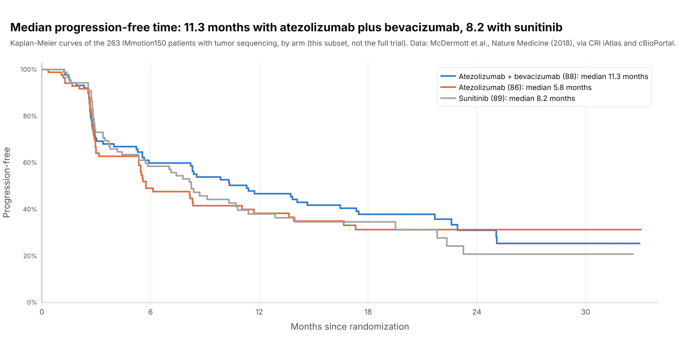
Another way to see it: Kaplan-Meier curves give each arm’s median, 11.3 months with atezolizumab plus bevacizumab against 8.2 with sunitinib in this subset, which is the comparison a randomized trial is designed for:

Kaplan-Meier curves of progression-free time for the three IMmotion150 arms: atezolizumab plus bevacizumab in blue with a median of 11.3 months, atezolizumab in orange at 5.8 months, and sunitinib in gray at 8.2 months

2. Why each patient stopped: buparlisib plus letrozole

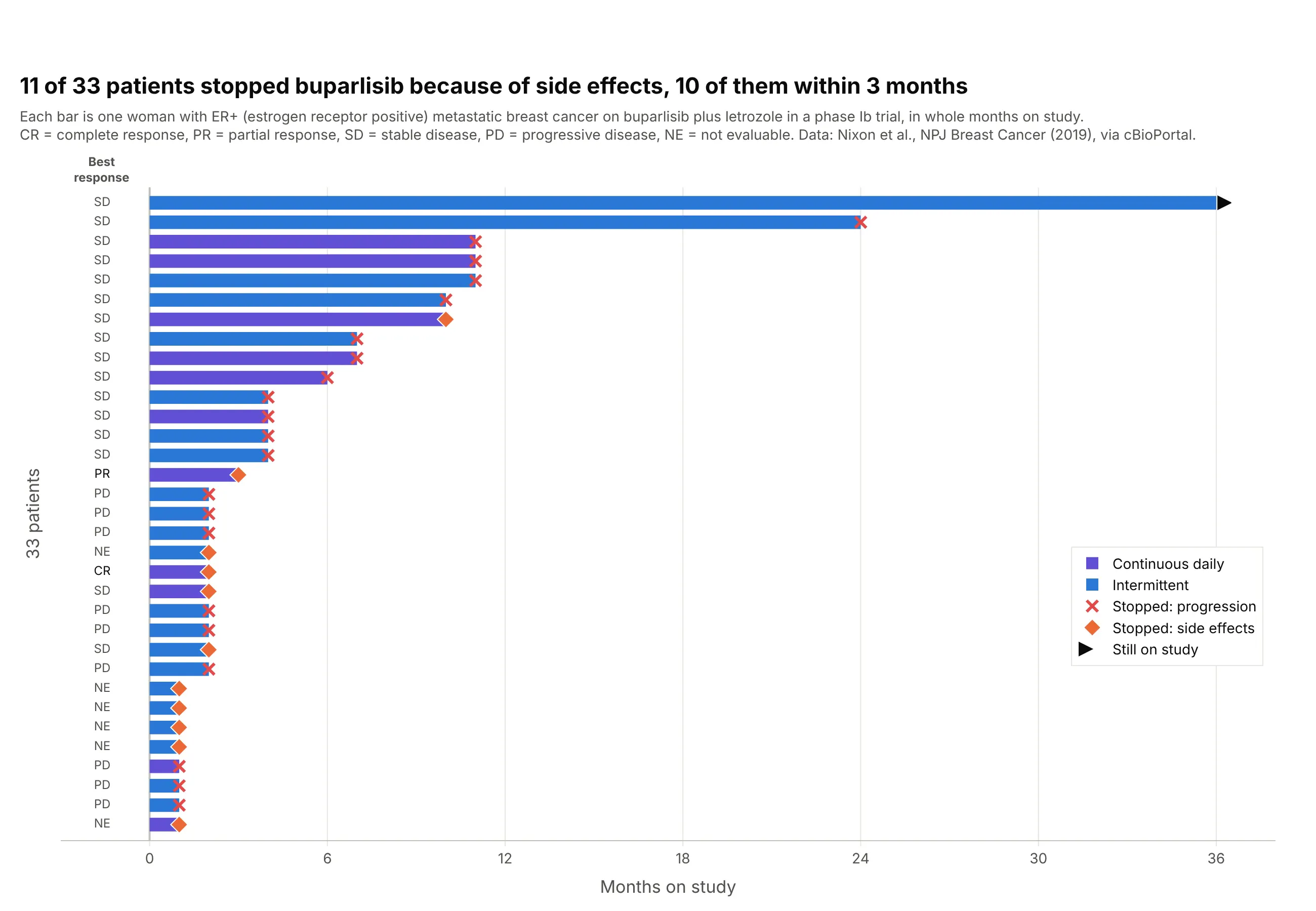
Swimmer plot of 33 women on buparlisib plus letrozole, bars colored by continuous or intermittent dosing, sorted by whole months on study, with red crosses for progression, orange diamonds for side effects at the end of 11 bars, mostly the shortest, and one arrow at 36 months

Eleven of 33 women in a phase Ib trial of buparlisib plus letrozole stopped because of side effects, 10 of them within three months, while progression ended most of the longer courses. Marking why each bar ends puts tolerability next to benefit. Data: Nixon et al. (2019), NPJ Breast Cancer, via cBioPortal.

Tip: use a different end-of-bar symbol for each reason treatment stopped, and keep red for progression.

Get the data from cBioPortal's study brca_mskcc_2019 (Nixon et al., NPJ Breast Cancer 2019; patients with THERAPY =
BKM120, attributes STUDY_ARM, MONTHS_ON_STUDY, BEST_RESPONSE_TO_THERAPY, REASON_FOR_TX_DISCONTINUATION) and shape it
into a table (columns: patient, schedule, months_on_study, best_response, stop_reason).

Build a plotly swimmer plot sorted by months_on_study, colored by schedule, with an end-of-bar marker per stop_reason,
an arrow for the patient still on study and the best response as a text column at the left.

3. Every patient, grouped by best response

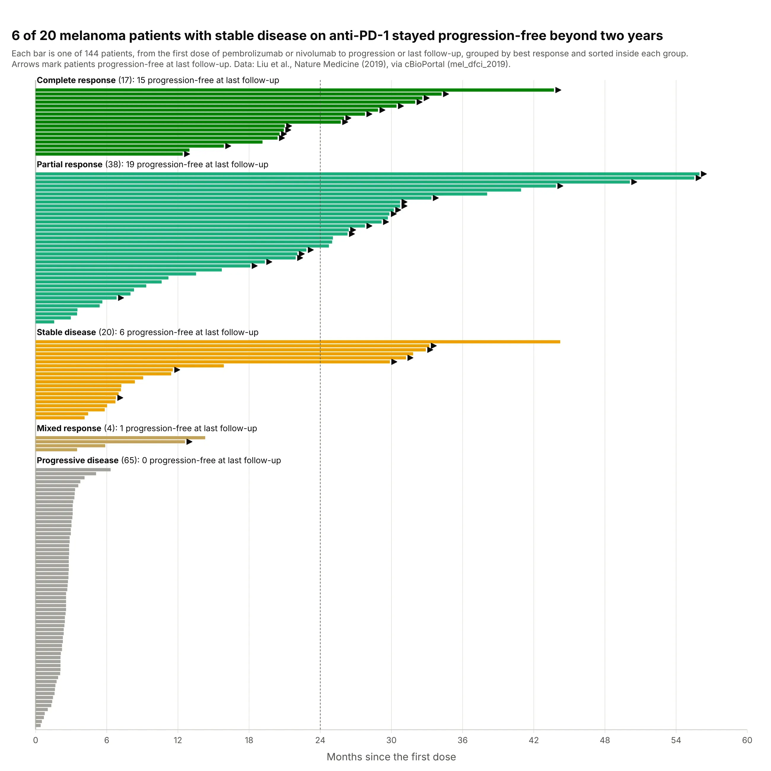
Swimmer plot of all 144 anti-PD-1 melanoma patients in five blocks, complete response 17, partial response 38, stable disease 20, mixed response 4, and progressive disease 65, each sorted by progression-free months, with arrows on patients still progression-free; six stable disease bars pass the 2-year line

Showing all 144 melanoma patients, not only the responders, puts the 65 with progressive disease in view, and it shows that six of the 20 with stable disease stayed progression-free beyond two years. Data: Liu et al. (2019), Nature Medicine, via cBioPortal.

Tip: group the bars by best response with a labeled gap between groups, and sort inside each group.

Get the data from cBioPortal's study mel_dfci_2019 (Liu et al., Nature Medicine 2019, 144 patients treated with
anti-PD-1; attributes BR, PFS_MONTHS, PFS_STATUS, IO_THERAPY) and shape it into a table (columns: patient, drug,
best_response, pfs_months, progressed).

Build a plotly swimmer plot with one block per best_response (complete, partial, stable, mixed, progressive), sorted
inside each block, a gap and a label above each block, and arrows for patients without progression.

4. Every US nuclear reactor, from its first day of commercial operation

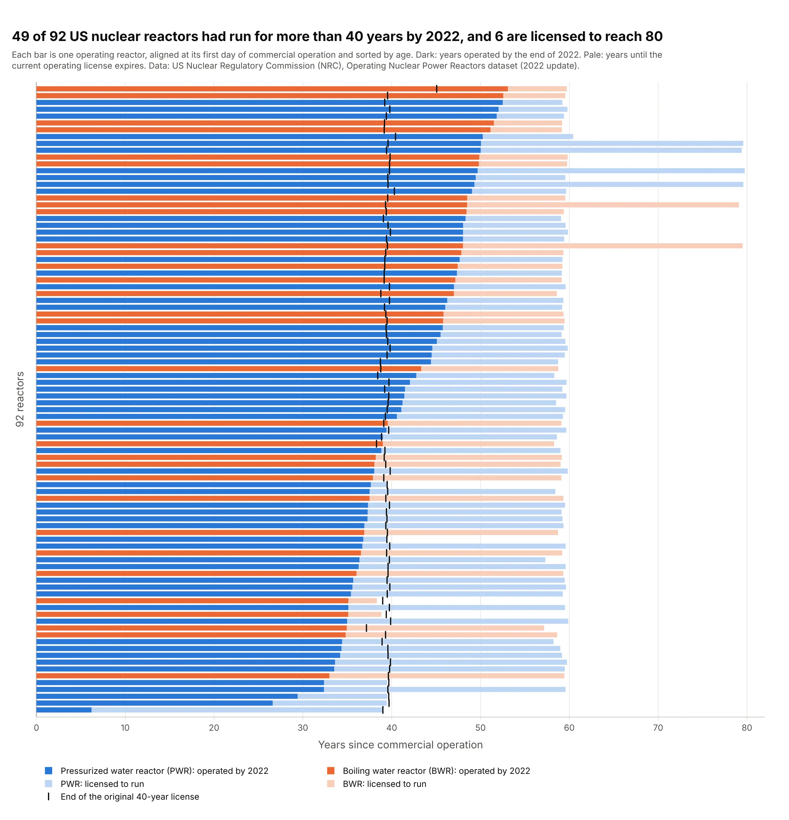
Swimmer plot of 92 US nuclear reactors aligned at commercial operation and sorted by age: dark blue and orange bars for years operated by 2022 for pressurized and boiling water reactors, pale extensions to the license expiry mostly near 60 years and 6 reaching about 80, and a black tick near 40 years on every bar

Forty-nine of the 92 operating US reactors had run for more than 40 years, their original license term, by the end of 2022, and six now hold licenses to reach about 80. Lining the reactors up at their first day of commercial operation does what a swimmer plot does with each patient’s first dose. Data: US Nuclear Regulatory Commission (NRC), Operating Nuclear Power Reactors dataset (2022 update).

Tip: draw time already used as a dark bar and time still planned as a pale bar behind it, both from zero.

Get the data from the NRC's "Operating Nuclear Power Reactors" dataset (nrc.gov reading room datasets,
reactors-operating.xlsx, one row per reactor) and shape it into a table (columns: reactor, type, commercial_operation,
license_issued, license_expires).

Build a plotly swimmer plot with one bar per reactor from commercial operation: dark for years operated to the end of
2022, pale for years to license expiry, colored by PWR or BWR, a tick at the original 40-year license end, sorted by age.

5. NASA’s Mars rovers and landers against their planned missions

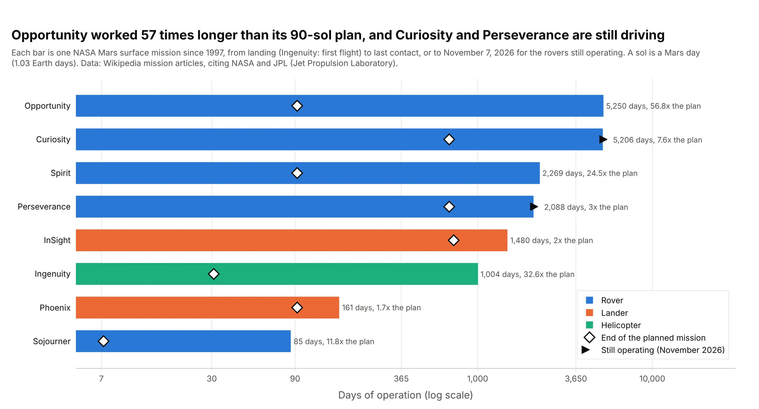
Swimmer plot on a log axis of 8 NASA Mars surface missions from Sojourner’s 85 days to Opportunity’s 5,250, bars colored by rover, lander, or helicopter, white diamonds at the end of each planned mission, arrows for Curiosity and Perseverance, which are still operating, and labels of the multiple of the plan

Opportunity was planned for 90 sols (Mars days) and worked for 5,250 Earth days, 57 times longer, and the Ingenuity helicopter flew 72 times over 1,004 days after a 30-sol demonstration plan. Curiosity and Perseverance are still driving, so their bars end in arrows like a patient still on treatment. Data: NASA and JPL (Jet Propulsion Laboratory) mission records, via the Wikipedia articles on each mission.

Tip: when durations span orders of magnitude, use a log x axis and print the number at the end of each bar.

Get the data from NASA's mission pages and the Wikipedia article for each NASA Mars surface mission since 1997
(Sojourner, Spirit, Opportunity, Phoenix, Curiosity, InSight, Perseverance, Ingenuity: landing or first-flight date,
last contact, planned primary mission in sols) and shape it into a table (columns: mission, kind, start, end,
planned_days, actual_days).

Build a plotly swimmer plot on a log x axis, bars sorted by actual_days and colored by kind, a diamond at planned_days,
arrows for missions still operating and the ratio of actual to planned at the end of each bar.

6. How long each Python release is supported

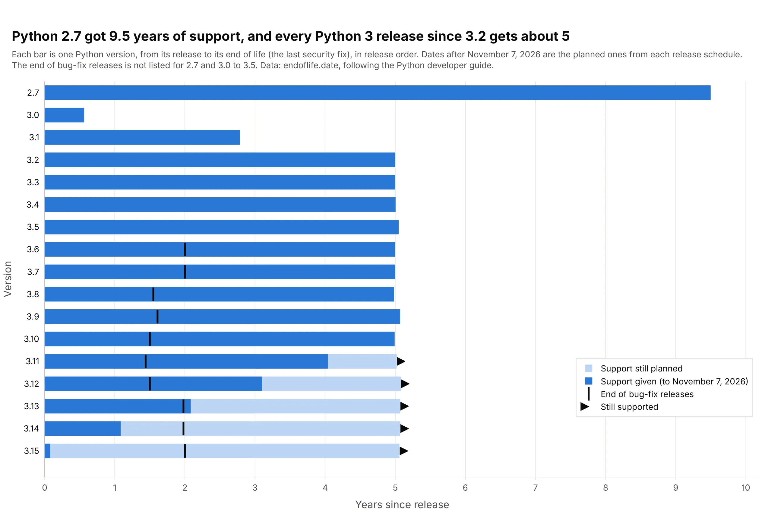
Swimmer plot of Python 2.7 and 3.0 to 3.15 in release order: dark bars for support already given, pale bars for support still planned, a black tick where bug-fix releases end between 1.4 and 2 years, arrows on 3.11 to 3.15, and 2.7’s bar reaching 9.5 years

Python 2.7 was supported for 9.5 years, from July 2010 to January 2020, and every Python 3 release since 3.2 gets about five years, with bug-fix releases for the first 1.4 to 2 of them. The versions with arrows, 3.11 to 3.15, are the ones still supported in November 2026. Data: endoflife.date, following the Python developer guide.

Tip: when the rows have a natural order, such as versions or cohorts, keep it instead of sorting by length.

Get the data from endoflife.date's Python API (endoflife.date/api/python.json, one row per release cycle with
releaseDate, support for the end of bug fixes and eol for end of life) and shape it into a table (columns: version,
release, bugfix_end, eol).

Build a plotly swimmer plot with one bar per version in release order: dark for years already supported, pale for years
still planned, a tick at the end of bug fixes and an arrow for versions still supported.