Chris Parmer

November 3, 2026

Scatter Plots - A Complete Guide

TL;DR

A scatter plot draws one dot per item at the position of two numbers, one on each axis, so you can see whether they move together, how tightly, and which items break the pattern.
Scatter plots are also known as scatterplots, scatter graphs, scatter charts, scattergrams and scatter diagrams, and are similar to bubble charts, hexbin plots, scatter plot matrices, strip charts and beeswarm plots.
You can make a scatter plot with Plotly in one line of code with px.scatter, add a trendline with trendline="ols" or "lowess", and draw it in JavaScript or React with plotly.js.
Plotly draws a scatter plot as SVG or with WebGL (go.Scattergl), which handles millions of points; px.scatter switches to WebGL by itself above 1,000 rows.
See 13 ways to draw a scatter plot below, all on the same World Bank data, from a plain scatter plot to trendlines, marginal histograms, a 3D scatter plot and an animation.

What is a scatter plot?

Scatter plots look like this:

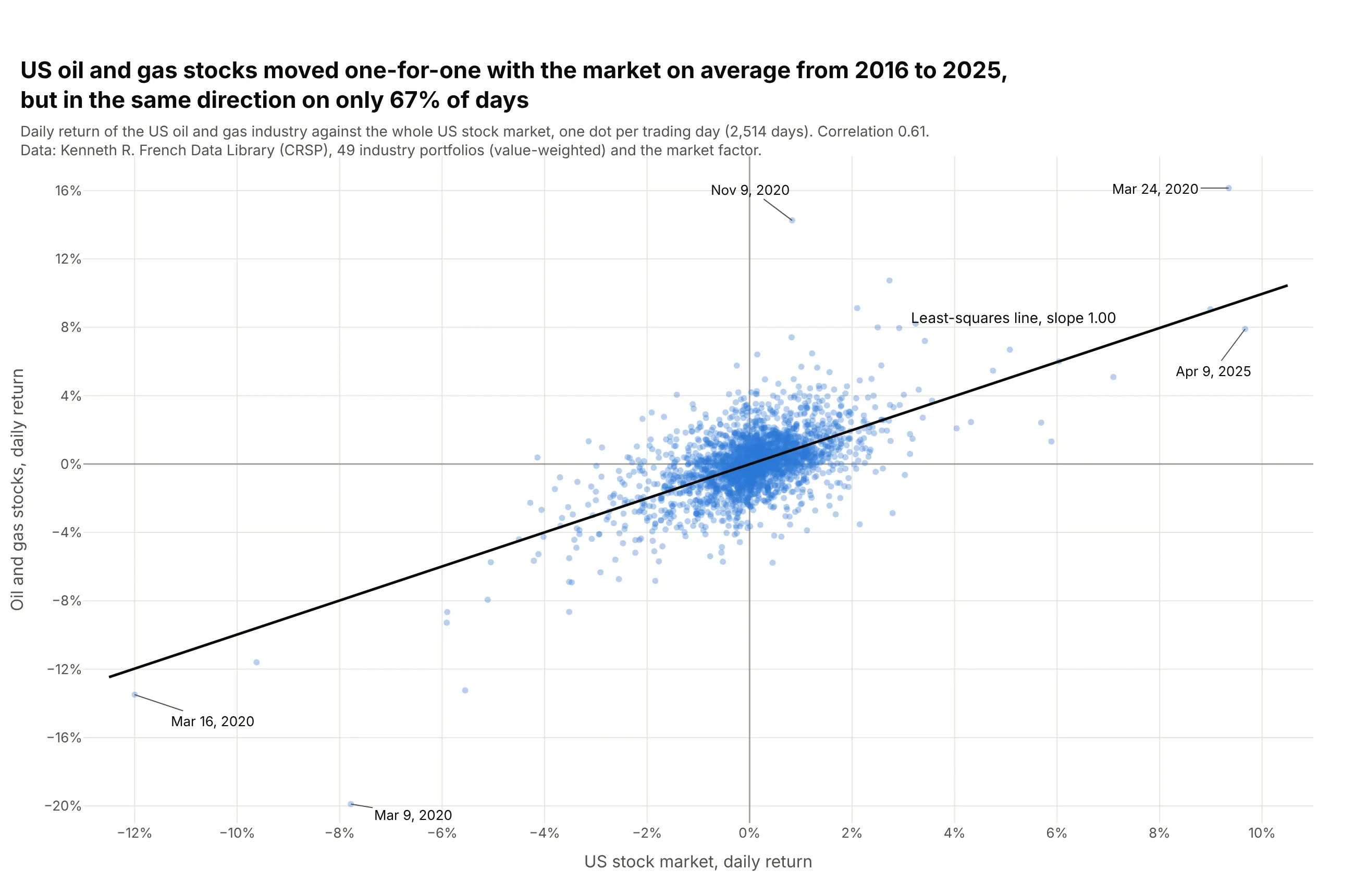
Scatter plot of 2,514 trading days from 2016 to 2025, the daily return of the whole US stock market on the x axis and of US oil and gas stocks on the y axis, a cloud of semi-transparent blue dots elongated from lower left to upper right with a black least-squares line of slope 1.00, and five extreme days labeled, including March 9, 2020 at -19.9% for oil

Data: Kenneth R. French Data Library (CRSP), 49 industry portfolios and the market factor, daily.

How do you read a scatter plot? In the example above, notice these things:

Each dot is one trading day, placed across by that day's return of the whole US stock market and up by the return of US oil and gas stocks.
The cloud runs from lower left to upper right, so the two usually moved together. The correlation is 0.61, and the two went the same way on 1,675 of 2,514 days (67%).
The black least-squares line has a slope of 1.00, which finance calls the industry's beta: on average, oil and gas stocks moved one-for-one with the market.
The cloud is taller than it is wide. Oil and gas stocks moved more than 5% on 47 days, and the market on 16, so much of their movement had nothing to do with the market.
The labeled dots are the days that break the pattern. On March 9, 2020 the market fell 7.8% and oil and gas stocks 19.9%, and on November 9, 2020 oil and gas rose 14.3% on a day the market rose 0.8%.

It's often used for charts like these:

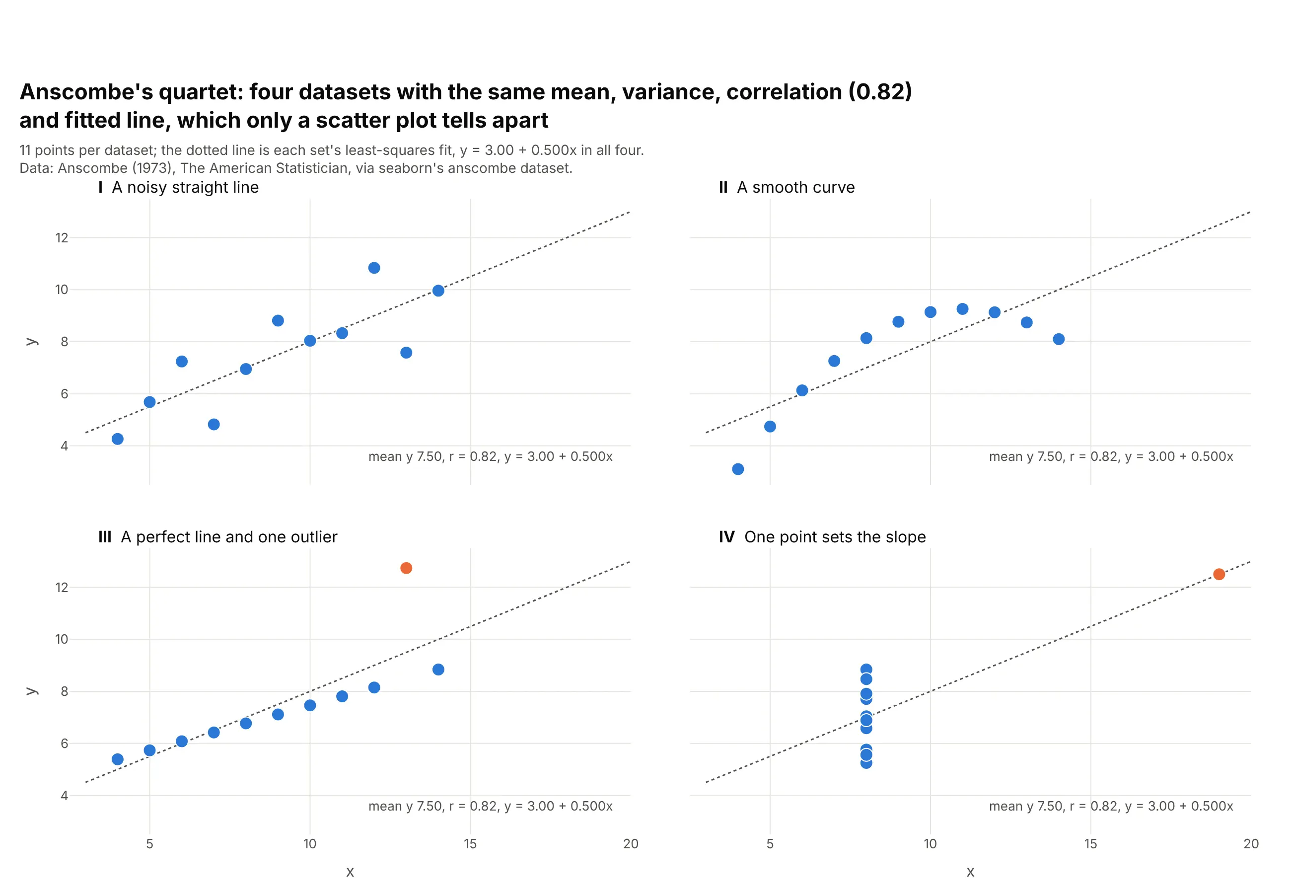
Anscombe's quartet as four scatter plots in a 2 x 2 grid: a noisy straight line, a smooth curve, a perfect line with one outlier in orange, and ten points in a vertical column with one far-right point in orange that sets the slope. Each panel has the same dotted fitted line, y = 3.00 + 0.500x, and correlation 0.82

Checking a correlation before you trust it. Anscombe built four datasets that share their means, variances, correlation (0.82) and fitted line, and only the scatter plots show that one is a curve and two depend on a single point. Data: Anscombe (1973), seaborn's anscombe dataset.

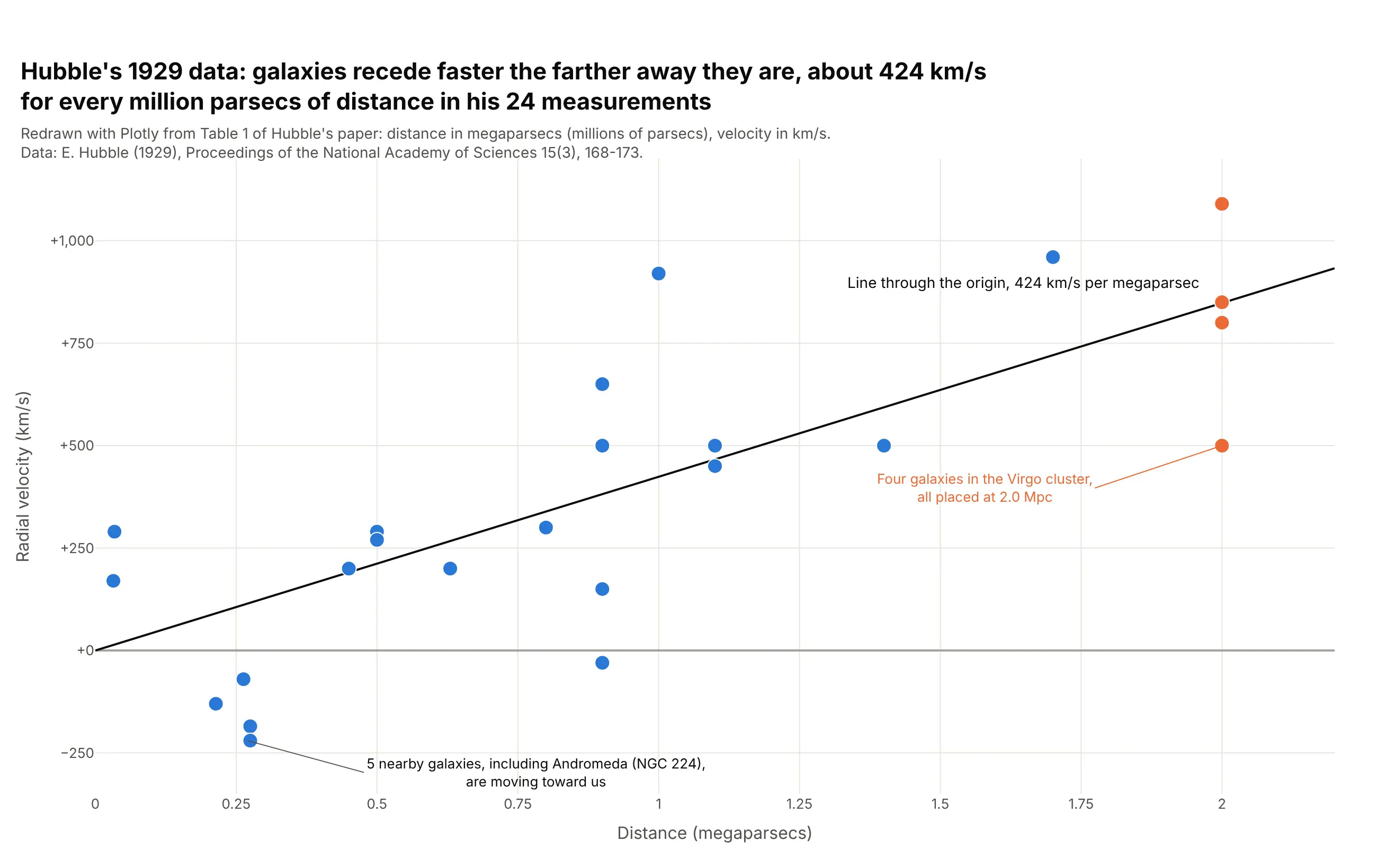
Redraw of Hubble's 1929 data: 24 galaxies with distance in megaparsecs on the x axis and radial velocity in km/s on the y axis, rising from negative velocities near zero distance to about 1,000 km/s at 2 megaparsecs, with a black line through the origin at 424 km/s per megaparsec and the four Virgo cluster galaxies at 2.0 Mpc in orange

Discovering a law in measurements. Hubble's 24 galaxies recede faster the farther away they are, about 424 km/s for every megaparsec in a least-squares line through the origin, the relationship now called Hubble's law. Data: Hubble (1929), Table 1.

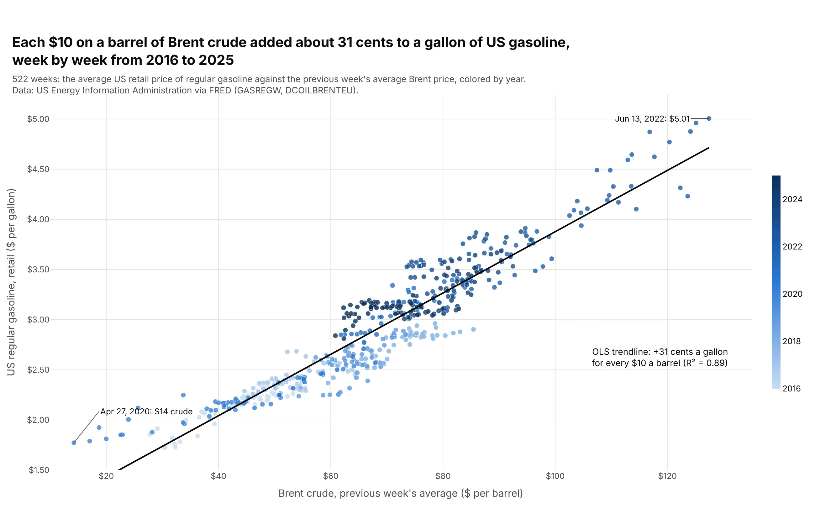
Scatter plot of 522 weeks from 2016 to 2025, Brent crude price on the x axis and US retail gasoline price on the y axis, dots shaded from light blue in 2016 to dark blue in 2025 along a black OLS trendline, with June 13, 2022 at $5.01 labeled

Measuring how one price passes into another. From 2016 to 2025, each $10 on a barrel of Brent crude went with about 31 cents on a gallon of US gasoline, along a trendline with an R² of 0.89. Data: US Energy Information Administration via FRED (GASREGW, DCOILBRENTEU).

A short history

Friendly and Denis's history of the chart (2005) credits John Herschel with the first true scatter plot, in an 1833 study of the double star Gamma Virginis, and the chart became a statistical tool with Francis Galton's 1886 study of the heights of parents and their adult children (Galton 1886). Galton printed his data as a table of counts and drew smooth ellipses through it. This is his data redrawn as a scatter plot:

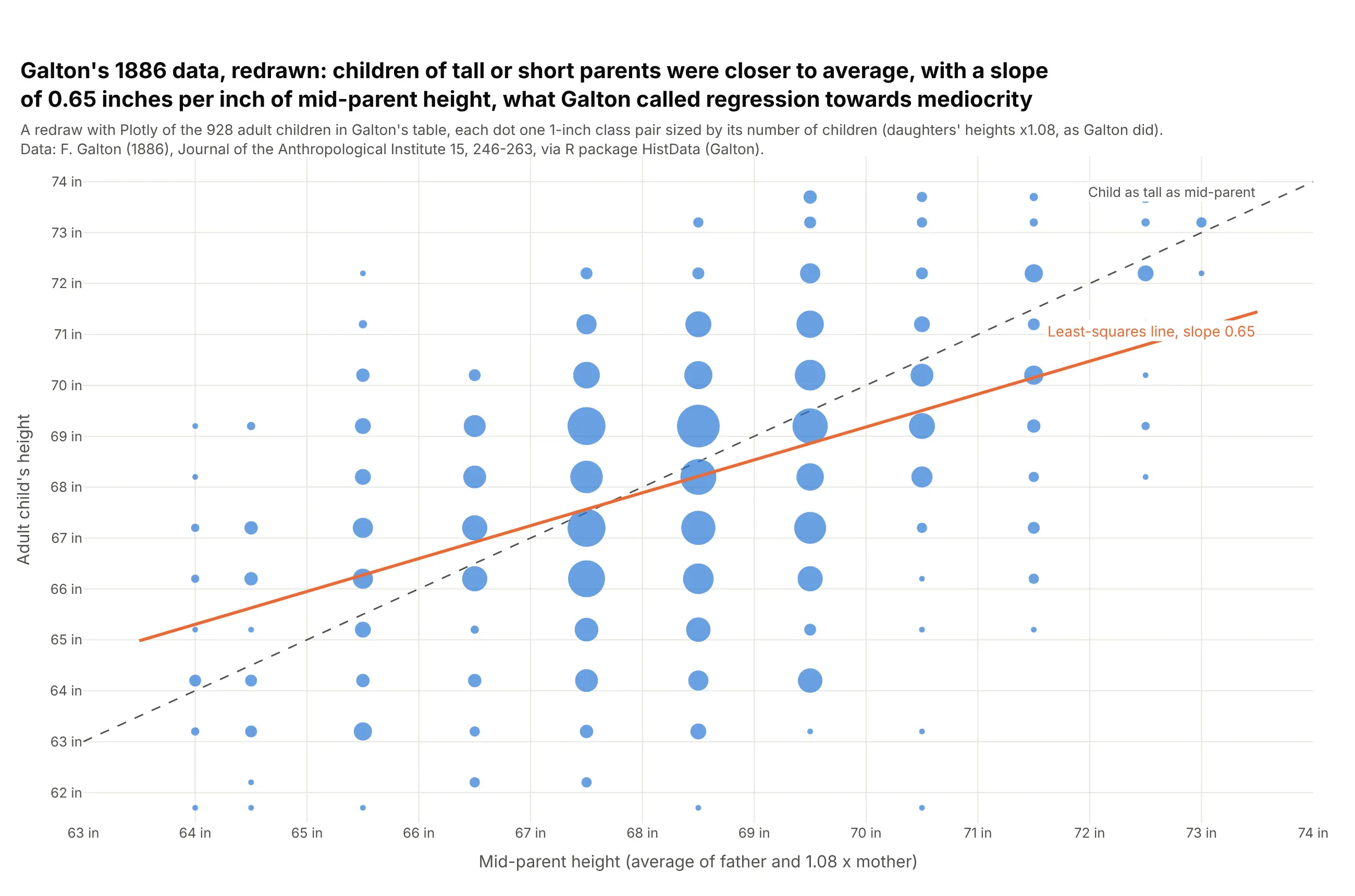
A redraw of Galton's 1886 data with Plotly: 928 adult children by mid-parent height and their own height in inches, each dot one 1-inch class pair sized by its count, with a dashed line where a child is as tall as the mid-parent and an orange least-squares line of slope 0.65 that is flatter than it

Data: Galton (1886) via R package HistData (Galton).

The orange line is flatter than the dashed one. Children of mid-parents 72.5 inches or taller averaged 72.1 inches, and children of mid-parents 64.5 inches or shorter averaged 65.4, so both groups were closer to the average than their parents, which Galton called regression towards mediocrity. The statistical term regression comes from this paper.

Alternatives to a scatter plot

Here's the same oil-and-market data drawn six ways. Some are better for the question, some worse, some just different:

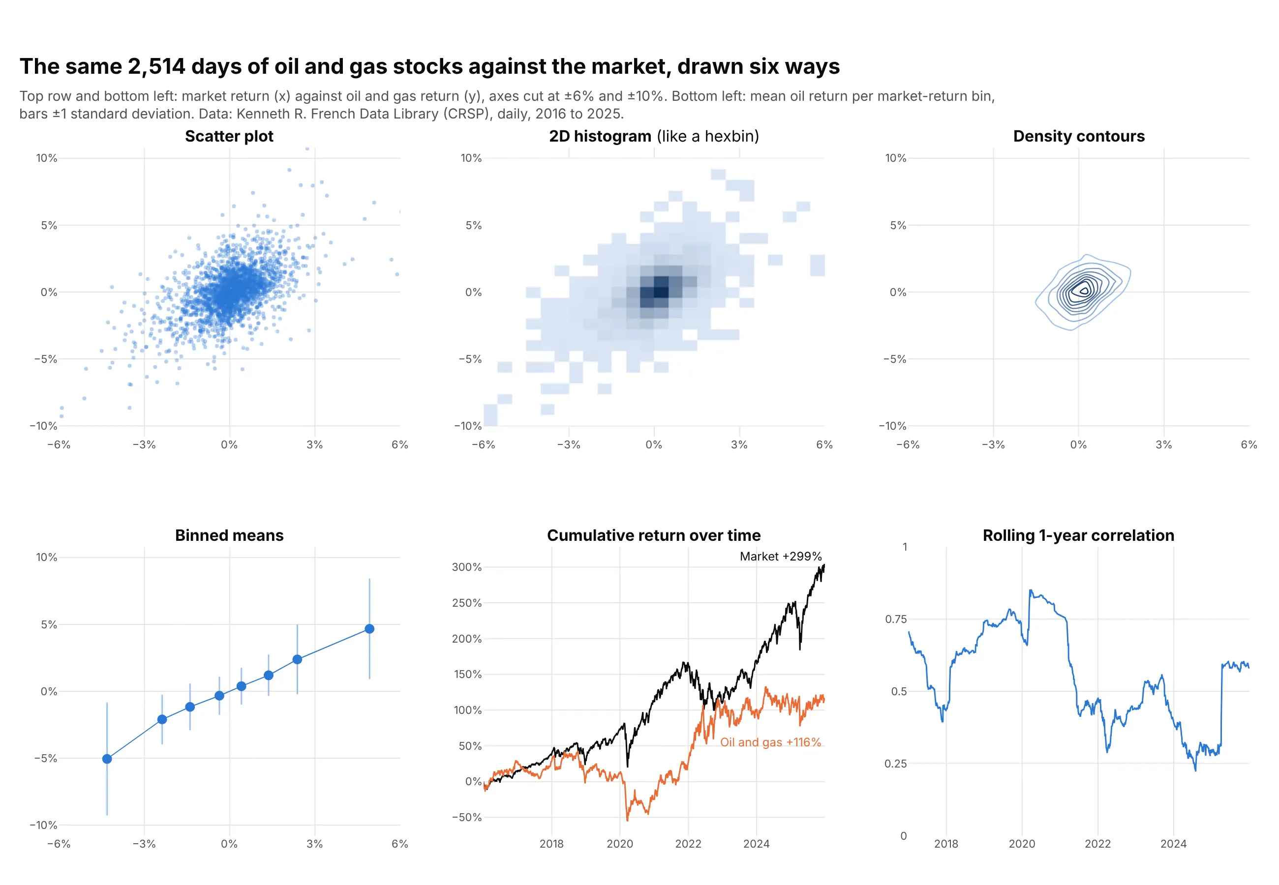
The 2,514 days of oil and gas stocks against the market drawn six ways: a scatter plot, a 2D histogram whose darkest cells sit at zero, density contours around the center, binned means rising from -5.05% to +4.67%, cumulative return lines ending at +299% for the market and +116% for oil and gas, and a rolling one-year correlation between 0.22 and 0.85

Scatter plot (better for seeing every day and the outliers). It shows the shape of the cloud, its slope and every extreme day, and hovering a dot gives its date.
Hexbin plot or 2D histogram (better above about 10,000 points). Counting points per cell shows where the data piles up, which a scatter plot of millions of points hides in a solid blob, but single outliers fade into faint cells.
Contour plot of density (different). Contours outline the dense core cleanly and work well over a scatter plot, though here most of the chart is empty and the extreme days disappear.
Binned means (better for the average relationship). Averaging the oil return in bins of market return shows the slope of about one without the noise, with bars for the spread, but it hides how many days sit in each bin.
Line chart over time (different question). Cumulative returns show that the market gained 299% and oil and gas 116% over the ten years, which the scatter plot can't show, because it drops the order of the days.
Rolling correlation (different question). One line shows the relationship changing, from 0.85 in 2020 to 0.22 in 2024, which a single scatter plot of ten years averages away.

For more than two numbers per item, a bubble chart adds a third as marker size and a scatter plot matrix draws every pair. For one number per item, a strip chart (a one-dimensional scatter plot) or a beeswarm plot shows each value as a dot along a single axis.

How to make a scatter plot

With AI

ChatGPT, Claude Code, GitHub Copilot, Cursor and other AI tools are excellent at writing Plotly code. Name Plotly in the prompt, and say which column goes on each axis, whether you want a trendline and which points to label:

Make a plotly scatter plot from oil_vs_market.csv (columns: date, market, oil; daily returns in percent).

- Use px.scatter with x = market and y = oil, 6 px markers at 0.35 opacity, the date on hover.
- Add an OLS trendline (trendline="ols") in black and print its slope.
- Gray zero lines on both axes, percent tick suffixes, and axis titles with units.
- Label the five days farthest from the center with their dates.
- Fixed width and height, and a title that states the takeaway.

With Plotly Studio

Plotly Studio is a desktop app where you point an AI at a dataset and it builds charts and a Dash app around your questions. Ask for a scatter plot the same way:

Show a scatter plot of weekly US gasoline prices against the Brent crude price, colored by year, with an OLS trendline and its slope in cents per gallon for each $10 a barrel, and the highest week labeled.

Make a scatter plot in Python or JavaScript

This is the code AI tools write under the hood. In Python, px.scatter makes a scatter plot in one line of code, and trendline="ols" fits a least-squares line with statsmodels, the same idea as seaborn's regplot. The Plotly scatter plot documentation covers color, size and facets, and the trendline documentation covers OLS, LOWESS and moving averages:

import pandas as pd
import plotly.express as px

df = pd.read_csv("oil_vs_market.csv")  # date, market, oil (daily returns, %)

fig = px.scatter(df, x="market", y="oil", hover_name="date", trendline="ols", trendline_color_override="black",
                 labels={"market": "US stock market, daily return (%)", "oil": "Oil and gas stocks, daily return (%)"})
fig.update_traces(selector=dict(mode="markers"), marker=dict(size=6, opacity=0.35))
fig.show()

print(px.get_trendline_results(fig).px_fit_results.iloc[0].params)  # intercept and slope (the beta)

px.scatter returns a figure with a go.Scatter trace in mode="markers". Add marginal_x="histogram" and marginal_y="histogram" for histograms on the edges (like seaborn's jointplot), use px.scatter_3d for a 3D scatter plot, px.scatter_polar for a polar scatter chart, and render_mode="webgl" for hundreds of thousands of points.

In JavaScript, a plotly.js scatter chart is a scatter trace with mode: "markers". This one draws Hubble's 24 galaxies and the line through the origin:

<div id="chart"></div>
<script src="https://cdn.plot.ly/plotly-4.1.1.min.js"></script>
<script>
  // Hubble (1929), Table 1: distance in megaparsecs and radial velocity in km/s for 24 galaxies
  const distance = [0.032, 0.034, 0.214, 0.263, 0.275, 0.275, 0.45, 0.5, 0.5, 0.63, 0.8, 0.9,
                    0.9, 0.9, 0.9, 1.0, 1.1, 1.1, 1.4, 1.7, 2.0, 2.0, 2.0, 2.0];
  const velocity = [170, 290, -130, -70, -185, -220, 200, 290, 270, 200, 300, -30,
                    650, 150, 500, 920, 450, 500, 500, 960, 500, 850, 800, 1090];

  // least-squares line through the origin: K = sum(x*y) / sum(x*x)
  const k = distance.reduce((s, x, i) => s + x * velocity[i], 0) / distance.reduce((s, x) => s + x * x, 0);

  Plotly.newPlot("chart", [
    {type: "scatter", mode: "markers", x: distance, y: velocity, name: "Galaxies",
     marker: {size: 12, color: "#2a78d6", line: {width: 1, color: "white"}},
     hovertemplate: "%{x} Mpc, %{y} km/s<extra></extra>"},
    {type: "scatter", mode: "lines", x: [0, 2.2], y: [0, 2.2 * k], name: `${k.toFixed(0)} km/s per Mpc`,
     line: {color: "black", width: 2}}
  ], {
    width: 800, height: 500, margin: {l: 70, r: 20, t: 20, b: 50},
    xaxis: {title: {text: "Distance (megaparsecs)"}},
    yaxis: {title: {text: "Radial velocity (km/s)"}, zeroline: true},
    legend: {x: 0.02, y: 0.98}
  });
</script>

For a React scatter chart, the Plot component from react-plotly.js takes the same data and layout:

import Plot from "react-plotly.js";

export function ScatterChart({ points }) {  // points: [{date, market, oil}, ...]
  return (
    <Plot
      data={[{
        type: "scatter", mode: "markers",
        x: points.map(p => p.market), y: points.map(p => p.oil), text: points.map(p => p.date),
        marker: { size: 6, opacity: 0.4, color: "#2a78d6" },
        hovertemplate: "%{text}<br>Market %{x}%<br>Oil %{y}%<extra></extra>",
      }]}
      layout={{ xaxis: { title: { text: "Market return (%)" } }, yaxis: { title: { text: "Oil and gas return (%)" } } }}
      style={{ width: "100%", height: 450 }}
      useResizeHandler
    />
  );
}

Use type: "scattergl" in either one for very large datasets.

Share it

Every Plotly chart has a Share chart button (the cloud icon in its toolbar) that uploads it to Plotly Cloud and gives you a link. Only you can see it until you change its visibility.

For a live app, put the chart in a Dash app and publish it with the Plotly Cloud CLI. Coding agents can run these commands for you:

pip install "dash[cloud]"
plotly user login
plotly app publish

If your data has to stay in your own cloud or data center, publish to Dash Enterprise instead.

Dos and don'ts

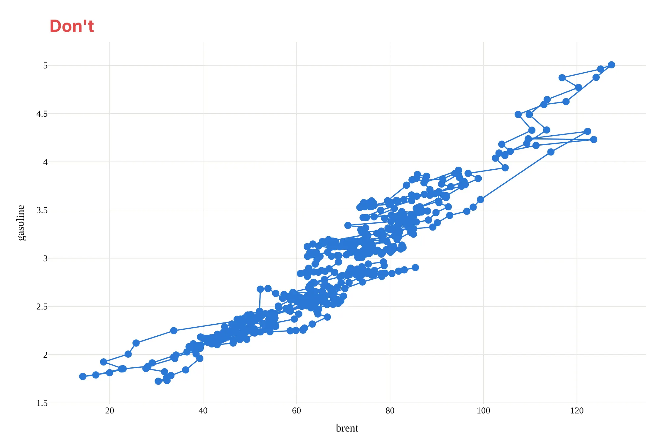
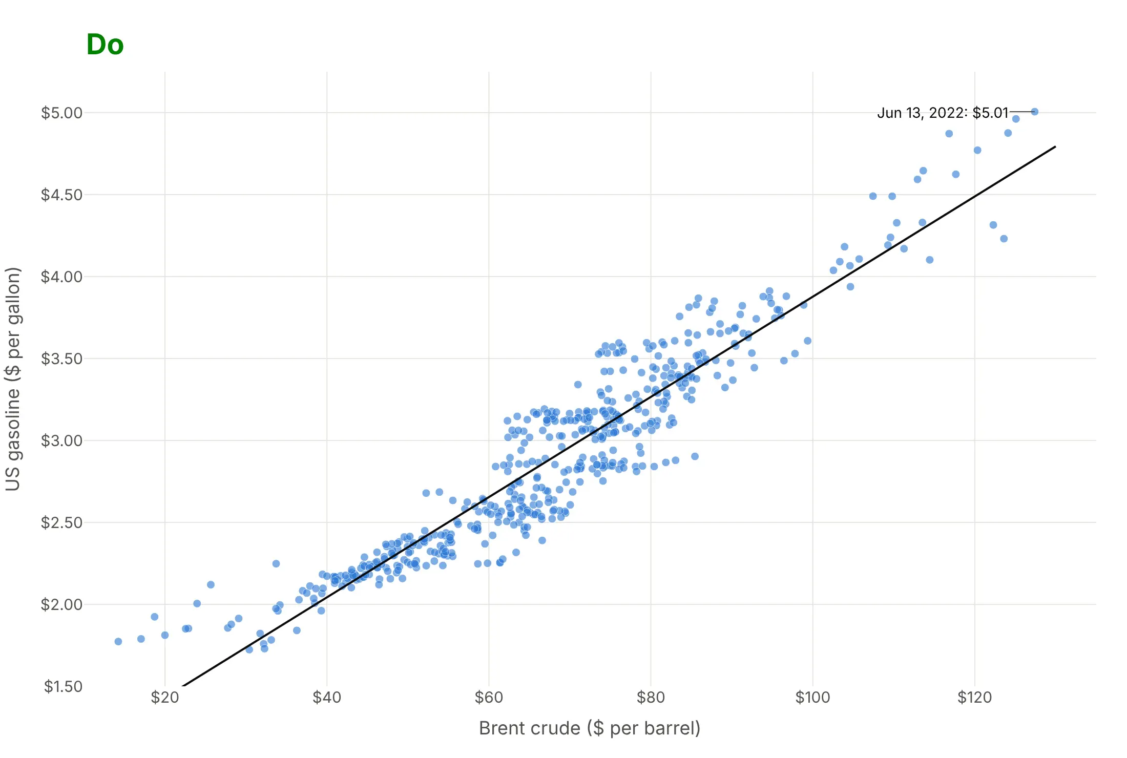
Most of the work in a published scatter plot is keeping the dots readable and the axes honest. Here are the 522 weeks of gasoline and crude prices both ways, in the same blue.

Don't join the points with lines (which draws the weeks in date order and turns the cloud into a tangle), use big opaque markers that hide each other, or use a default serif font, raw column names as axis titles and unformatted numbers:

The 522 weeks of gasoline against Brent drawn as large blue dots joined by lines in date order, a tangled scribble with a serif font, axis titles brent and gasoline, and plain numbers

Do draw markers only, small and partly transparent so dense areas look darker, add a trendline, put units in the axis titles, format the ticks as dollars and label the point the story needs:

The same 522 weeks as small semi-transparent blue dots with a black trendline, dollar ticks, axis titles with units and June 13, 2022 at $5.01 labeled

Checklist

Put the variable you think drives the other on the x axis.
Use small, partly transparent markers above a few hundred points, and WebGL above about 100,000.
Use a log axis when values span orders of magnitude, such as prices, populations or spending.
Add a trendline when the slope is the point, and say what kind (OLS or LOWESS) in the subtitle.
Label the few points the story needs, and put names in the hover text for the rest.
Write a title that states the relationship, with its number.

Don't

Read a correlation as cause. Health spending and life expectancy both rise with income, as the 3D scatter plot below shows.
Connect the points with lines unless the order means something (then it's a connected scatter plot, as in way 10 below).
Trust a correlation coefficient without the plot. Anscombe's quartet above has four different pictures behind the same 0.82.
Draw tens of thousands of opaque dots; switch to transparency, WebGL or a hexbin plot.

Options to customize

A scatter plot in Plotly is px.scatter or a go.Scatter trace with mode="markers", so these are the options that matter most. The full lists are in the px.scatter reference and the scatter trace reference.

x, y: the two numeric columns; put the explanatory one on x.
color: a category (one color per group) or a number (a color scale).
size, size_max: marker area from a third number, which makes a bubble chart.
symbol: marker shape by category, useful in print and for colorblind readers.
trendline: "ols" for a least-squares line, "lowess" for a smooth local fit, "rolling" or "ewm" for moving averages; trendline_options sets frac for LOWESS or log_x/log_y for OLS, and trendline_scope="overall" fits one line across all colors.
marginal_x, marginal_y: "histogram", "box", "violin" or "rug" on the edges.
facet_col, facet_row, facet_col_wrap: small multiples of scatter plots.
log_x, log_y: log axes for data spanning orders of magnitude.
hover_name, hover_data, hovertemplate: the item's name and details on hover.
text, textposition (with mode="markers+text") or add_annotation: labels on chosen points.
marker.opacity, marker.size, marker.line: transparency, size and outline, for overplotting.
animation_frame, animation_group: one frame per year or period, with play and pause buttons.
render_mode="webgl" or go.Scattergl: WebGL drawing for hundreds of thousands of points.
px.scatter_3d, px.scatter_polar, px.scatter_geo, px.scatter_map: the same idea in 3D, on polar axes and on maps.

13 ways to draw a scatter plot

The World Bank publishes health spending per person and life expectancy at birth for nearly every country since 2000. We took those 4,539 country-years, with each country's population and income, and drew them 13 ways. Each one answers a different question about the same numbers.

1. A plain scatter plot

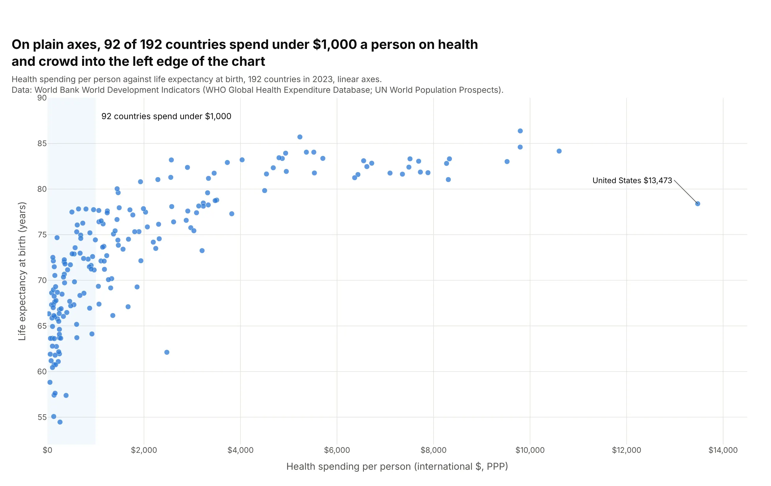
Scatter plot of 192 countries in 2023 with health spending per person on a linear x axis from $0 to $14,000 and life expectancy on the y axis, most dots crowded into a shaded band under $1,000 on the left and the United States alone at $13,473 on the right

The default px.scatter(df, x=..., y=...) puts each country at its spending and life expectancy. On linear axes the United States, at $13,473 a person, stretches the axis so far that 92 of 192 countries crowd into the first $1,000. It shows the overall rise and the bend in it, but hides almost everything about the poorer half of the world.

Prompt: Get the data from the World Bank World Development Indicators API: SH.XPD.CHEX.PP.CD (current health expenditure per capita, PPP) and SP.DYN.LE00.IN (life expectancy at birth) for 2023, countries only (columns: country, region, health_usd_ppp, life_exp). Make a plotly scatter plot with px.scatter, x = health_usd_ppp, y = life_exp, country on hover, 9 px markers, and shade the band under $1,000.

2. Log axis

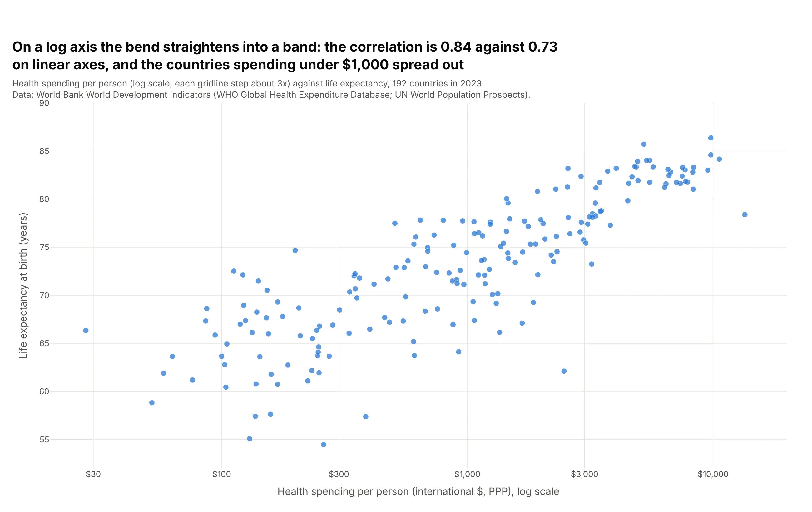
The same 192 countries with health spending on a log x axis from $30 to $10,000, the dots spread evenly into a rising band

With log_x=True, each step along the axis is a multiple of spending instead of a fixed number of dollars, and the bend becomes a straight band. The correlation rises from 0.73 on linear axes to 0.84 on log spending. Use a log axis whenever values span orders of magnitude; the cost is that readers have to notice the tick labels.

Prompt: Get the data from the World Bank World Development Indicators API (SH.XPD.CHEX.PP.CD and SP.DYN.LE00.IN, 2023, countries only). Make a plotly scatter plot with px.scatter and log_x=True, ticks at $30, $100, $300, $1,000, $3,000 and $10,000, and print the correlation of life expectancy with spending and with log10(spending).

3. Labeled outliers

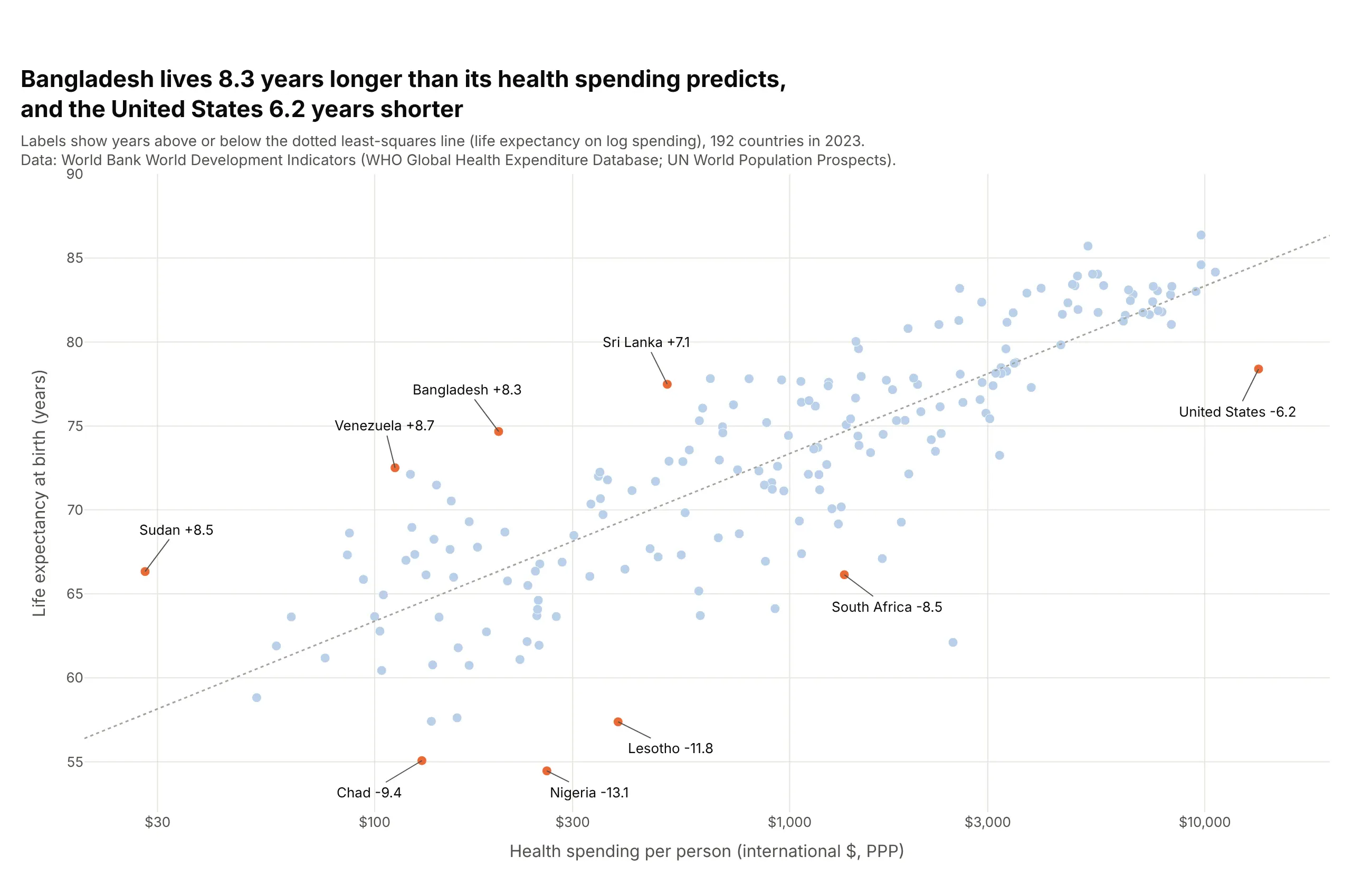
The log-axis scatter plot with a dotted least-squares line, most dots light blue and nine in orange with labels: Venezuela +8.7, Bangladesh +8.3, Sri Lanka +7.1 and Sudan +8.5 above the line, and Nigeria -13.1, Lesotho -11.8, Chad -9.4, South Africa -8.5 and the United States -6.2 below it

Labels turn a cloud into a story. Here each label is the distance from a least-squares line in years: Bangladesh, at $199 a person, lives 8.3 years longer than its spending predicts, and the United States 6.2 years shorter. Label only the points the reader needs, with add_annotation, and leave the rest to hover.

Prompt: Get the data from the World Bank World Development Indicators API (health spending per capita PPP and life expectancy, 2023). Fit life expectancy on log10(spending) with numpy.polyfit, compute each country's residual, and make a plotly scatter plot with a log x axis, light blue markers, the four largest positive and five largest negative residuals plus the United States in orange, and add_annotation labels showing each residual in years.

4. Color by group

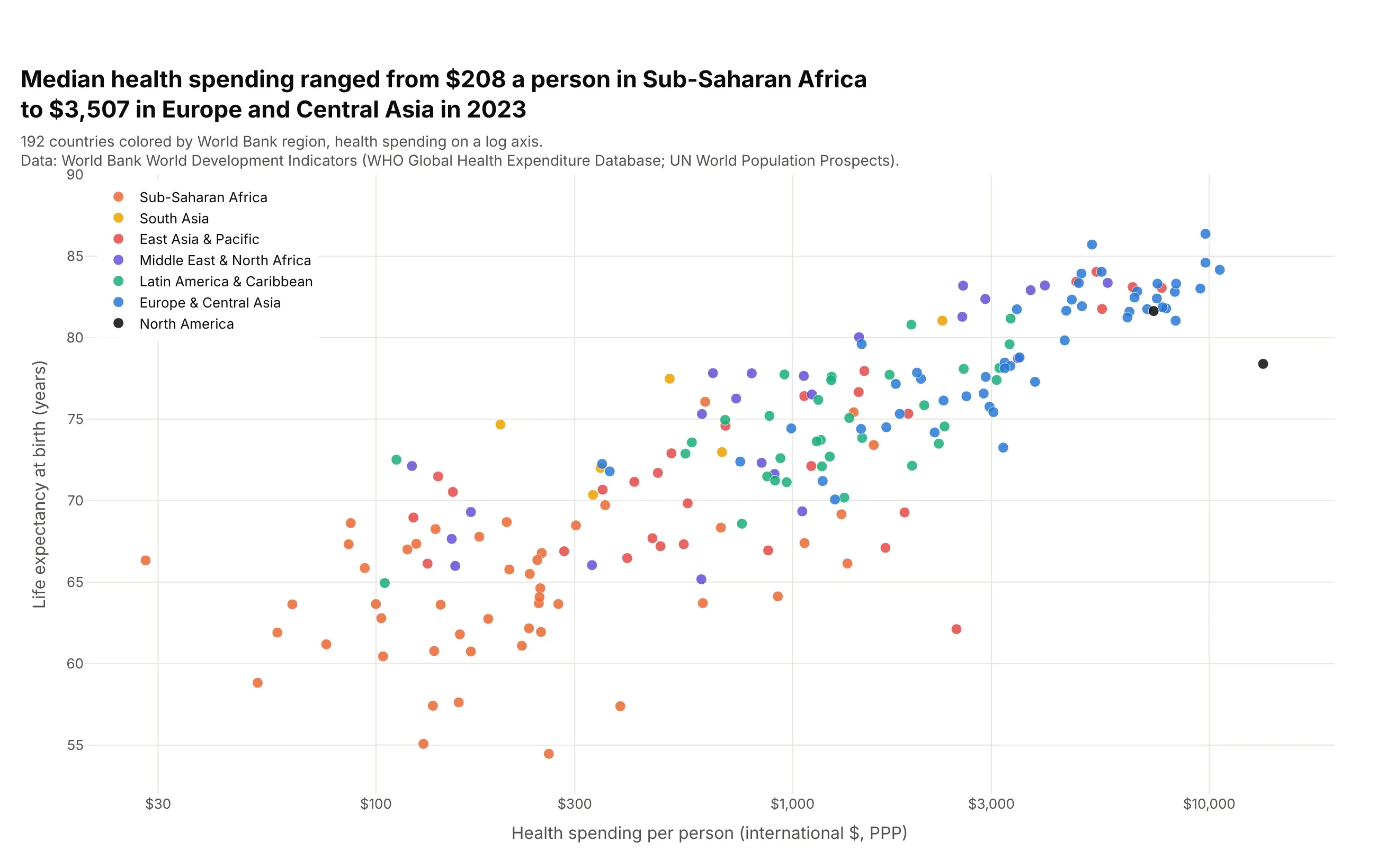
The log-axis scatter plot with each country colored by World Bank region, Sub-Saharan Africa in orange at the lower left and Europe and Central Asia in blue at the upper right, with a legend in the top left

color="region" gives each World Bank region its own color, and the regions sort themselves along the band: the median country spent $208 a person in Sub-Saharan Africa and $3,507 in Europe and Central Asia. Fix the order with category_orders and the colors with color_discrete_map, and keep it to about seven groups, because more colors stop being distinguishable.

Prompt: Get the data from the World Bank World Development Indicators API (SH.XPD.CHEX.PP.CD, SP.DYN.LE00.IN, 2023) with each country's World Bank region from the country endpoint. Make a plotly scatter plot with px.scatter, log_x=True, color="region", a fixed color_discrete_map and category_orders from the lowest-spending region to the highest, and the legend inside the top-left corner.

5. Size by a third number (a bubble chart)

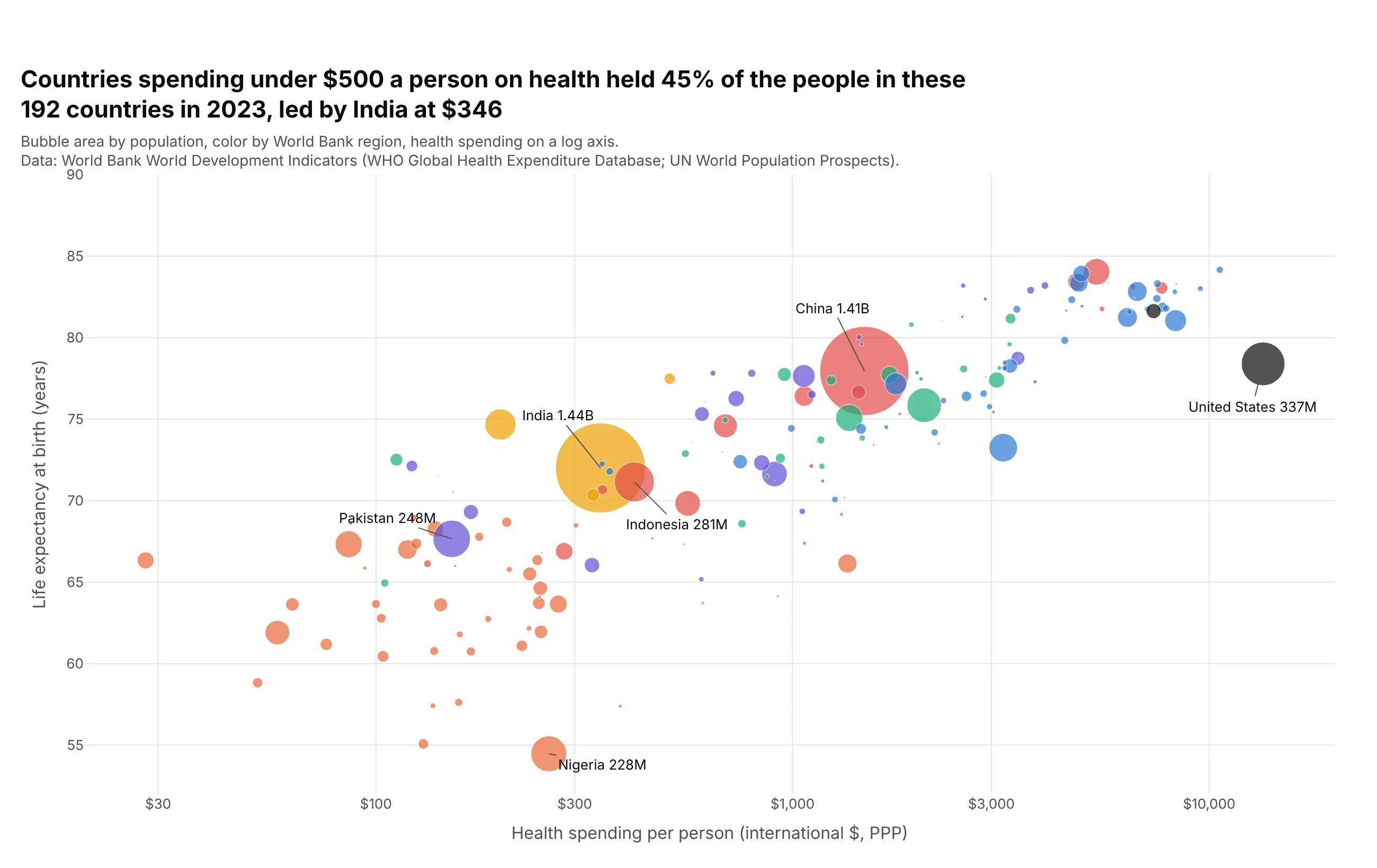
The log-axis scatter plot with bubble area by population, India's large yellow bubble at $346 and 72 years, China's large red bubble at $1,487 and 78 years, and Nigeria, Pakistan, Indonesia and the United States labeled with their populations

size="population" turns the scatter plot into a bubble chart, and the picture changes: countries spending under $500 a person held 45% of the people in these 192 countries in 2023, led by India at $346. Plotly sizes bubbles by area; size_max sets the largest. Big bubbles cover small ones, so sort the data so large countries are drawn first.

Prompt: Get the data from the World Bank World Development Indicators API (SH.XPD.CHEX.PP.CD, SP.DYN.LE00.IN, SP.POP.TOTL, 2023, countries only). Make a plotly bubble chart with px.scatter, log_x=True, size="population", size_max=60, color by World Bank region, data sorted by population descending, and the six most populous countries labeled with their populations.

6. OLS trendline

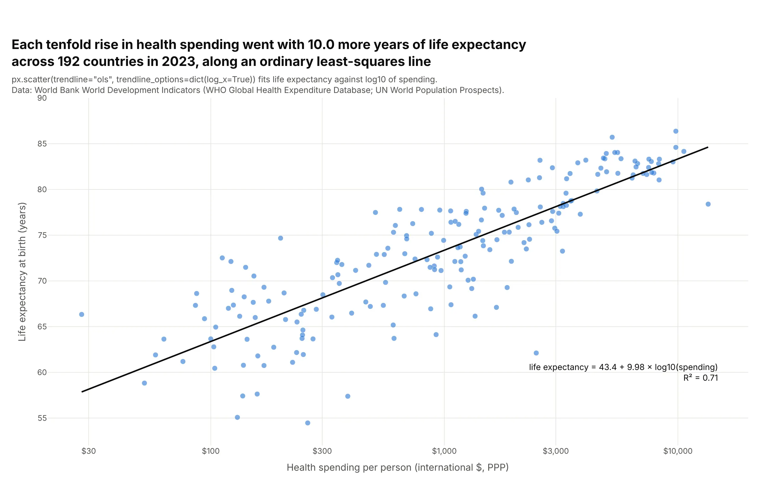
The log-axis scatter plot in blue with a black straight trendline rising from 58 years at $28 to 85 at $13,000, and the equation life expectancy = 43.4 + 9.98 × log10(spending), R² = 0.71

trendline="ols" fits an ordinary least-squares line with statsmodels, and trendline_options=dict(log_x=True) fits it against log spending so it's straight on a log axis. Each tenfold rise in spending went with 10.0 more years of life expectancy, and the line explains 71% of the variation (R² 0.71). px.get_trendline_results(fig) returns the fitted model with its coefficients and confidence intervals.

Prompt: Get the data from the World Bank World Development Indicators API (health spending per capita PPP and life expectancy at birth, 2023). Make a plotly scatter plot with px.scatter, log_x=True, trendline="ols", trendline_options=dict(log_x=True) and a black trendline, then read the slope and R² from px.get_trendline_results(fig) and print the equation on the chart.

7. LOWESS trendline

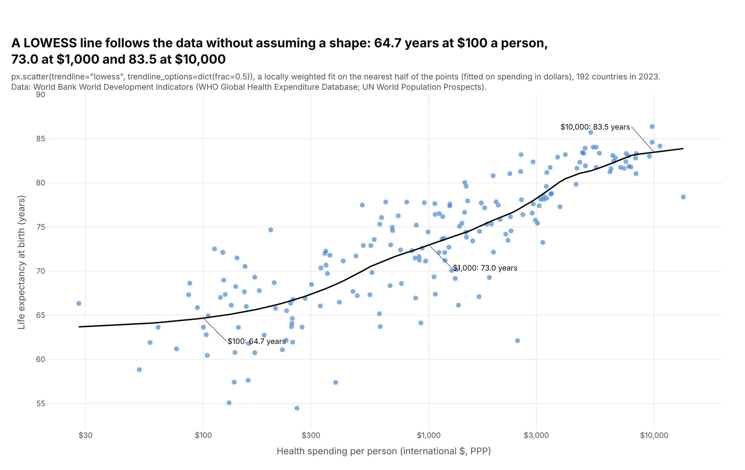
The log-axis scatter plot with a black curved LOWESS line, flat near 64 years below $100, rising through 73.0 years at $1,000 and leveling at 83.5 at $10,000, with those three points labeled

trendline="lowess" fits a locally weighted curve that follows the data without assuming a shape: 64.7 years at $100 a person, 73.0 at $1,000 and 83.5 at $10,000. It shows that life expectancy barely changes across the poorest countries and levels off among the richest, which a straight line hides. trendline_options=dict(frac=0.5) sets how much of the data each local fit uses; smaller values follow the points more closely.

Prompt: Get the data from the World Bank World Development Indicators API (SH.XPD.CHEX.PP.CD and SP.DYN.LE00.IN for 2023, countries only). Make a plotly scatter plot with px.scatter, log_x=True, trendline="lowess", trendline_options=dict(frac=0.5) and a black trendline, then read the fitted curve from fig.data[1] and label its value at $100, $1,000 and $10,000.

8. Marginal distributions

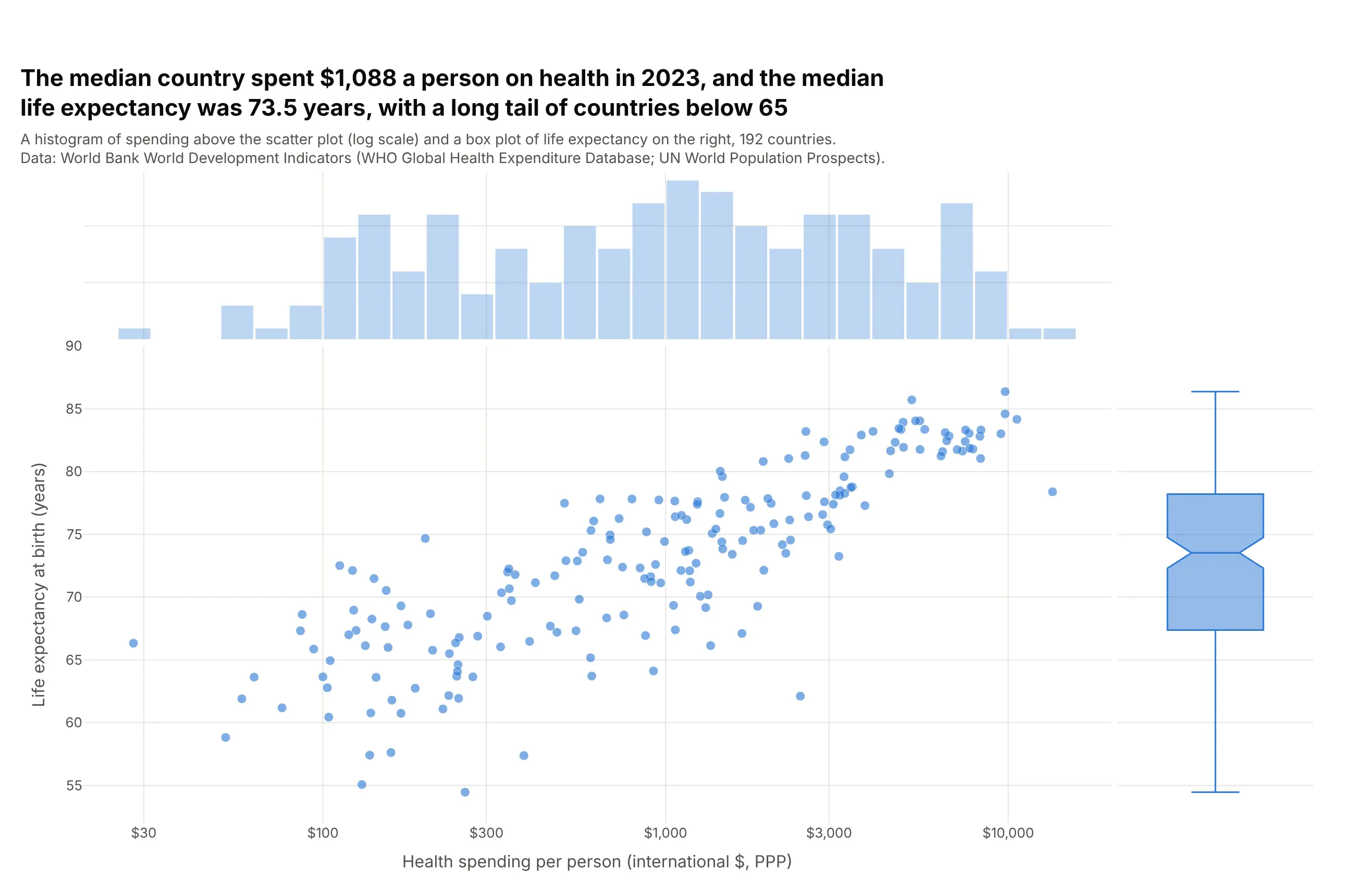
The log-axis scatter plot with a histogram of spending along the top and a box plot of life expectancy on the right, the box spanning about 67 to 78 years with a median of 73.5

marginal_x="histogram" and marginal_y="box" add each variable's distribution on the edges, like seaborn's jointplot. The median country spent $1,088 a person, and the box shows the median life expectancy of 73.5 years and a long lower tail, with 28 countries below 65. Plotly also offers "violin" and "rug" marginals. Because plotly.js histograms bin in linear units, this chart plots log10(spending) on a linear axis with dollar tick labels.

Prompt: Get the data from the World Bank World Development Indicators API (health spending per capita PPP and life expectancy, 2023). Add a column log_health = log10(health_usd_ppp). Make a plotly scatter plot with px.scatter, x = log_health, y = life_exp, marginal_x="histogram" with 0.1-wide bins, marginal_y="box", and x tick labels in dollars ($30 to $10,000) at the log10 positions.

9. Small multiples

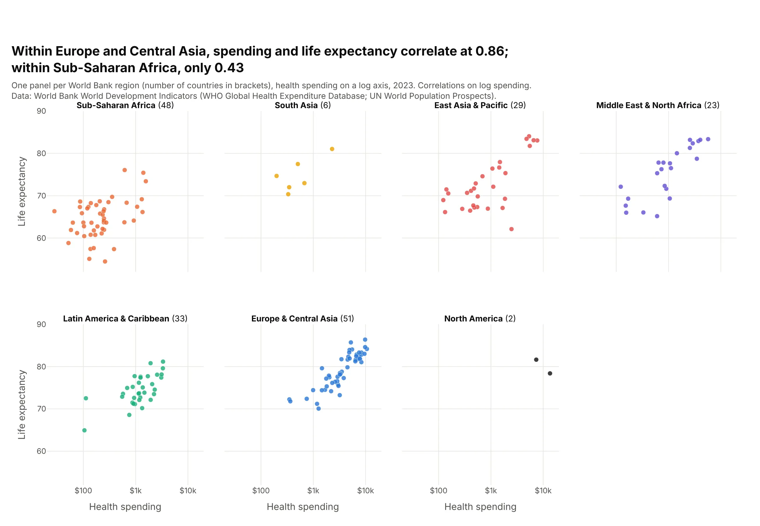
Seven scatter plots, one per World Bank region with the number of countries in brackets, sharing a log spending axis and a life expectancy axis: Europe and Central Asia (51) is a tight rising line and Sub-Saharan Africa (48) a loose cloud

facet_col="region" with facet_col_wrap=4 draws one scatter plot per region on shared axes. Within Europe and Central Asia, spending and life expectancy correlate at 0.86; within Sub-Saharan Africa, only 0.43. Facets keep groups from hiding behind each other, at the cost of smaller panels.

Prompt: Get the data from the World Bank World Development Indicators API (SH.XPD.CHEX.PP.CD, SP.DYN.LE00.IN, 2023) with World Bank regions. Make plotly small multiples with px.scatter, log_x=True, facet_col="region", facet_col_wrap=4, color by region, shared axes, panel titles with the number of countries, and print the correlation of life expectancy with log spending in each region.

10. Connected scatter plot

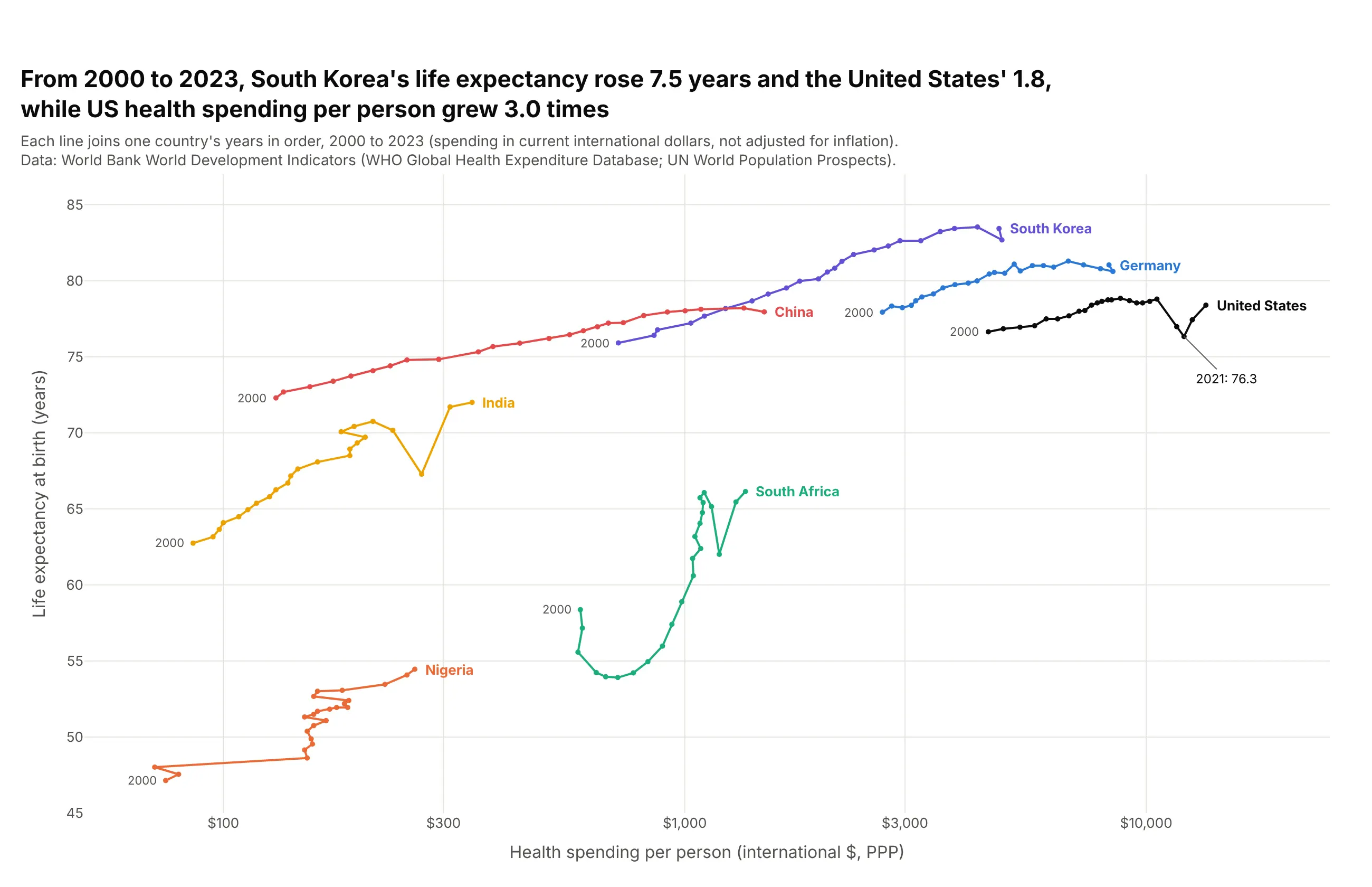
Seven lines tracing countries' paths from 2000 to 2023: South Korea rising steeply to 83.4 years, Germany and the United States moving right with little gain and a US dip to 76.3 in 2021, China and India rising, South Africa falling to 53.9 then recovering, and Nigeria rising slowly from 47 years

Joining one country's years in order, with mode="lines+markers", shows the path it took. From 2000 to 2023, South Korea's life expectancy rose 7.5 years and the United States' 1.8, while US spending per person grew 3.0 times in current dollars, with a dip to 76.3 years in 2021. Sort by year before drawing, and keep it to a handful of countries, or the paths tangle.

Prompt: Get the data from the World Bank World Development Indicators API (SH.XPD.CHEX.PP.CD and SP.DYN.LE00.IN, 2000-2023) for the United States, Germany, South Korea, China, India, South Africa and Nigeria. Make a plotly connected scatter plot: one go.Scatter per country with mode="lines+markers", rows sorted by year, a log x axis, the country name at the end of each path and "2000" at its start.

11. Every year at once, with WebGL and density contours

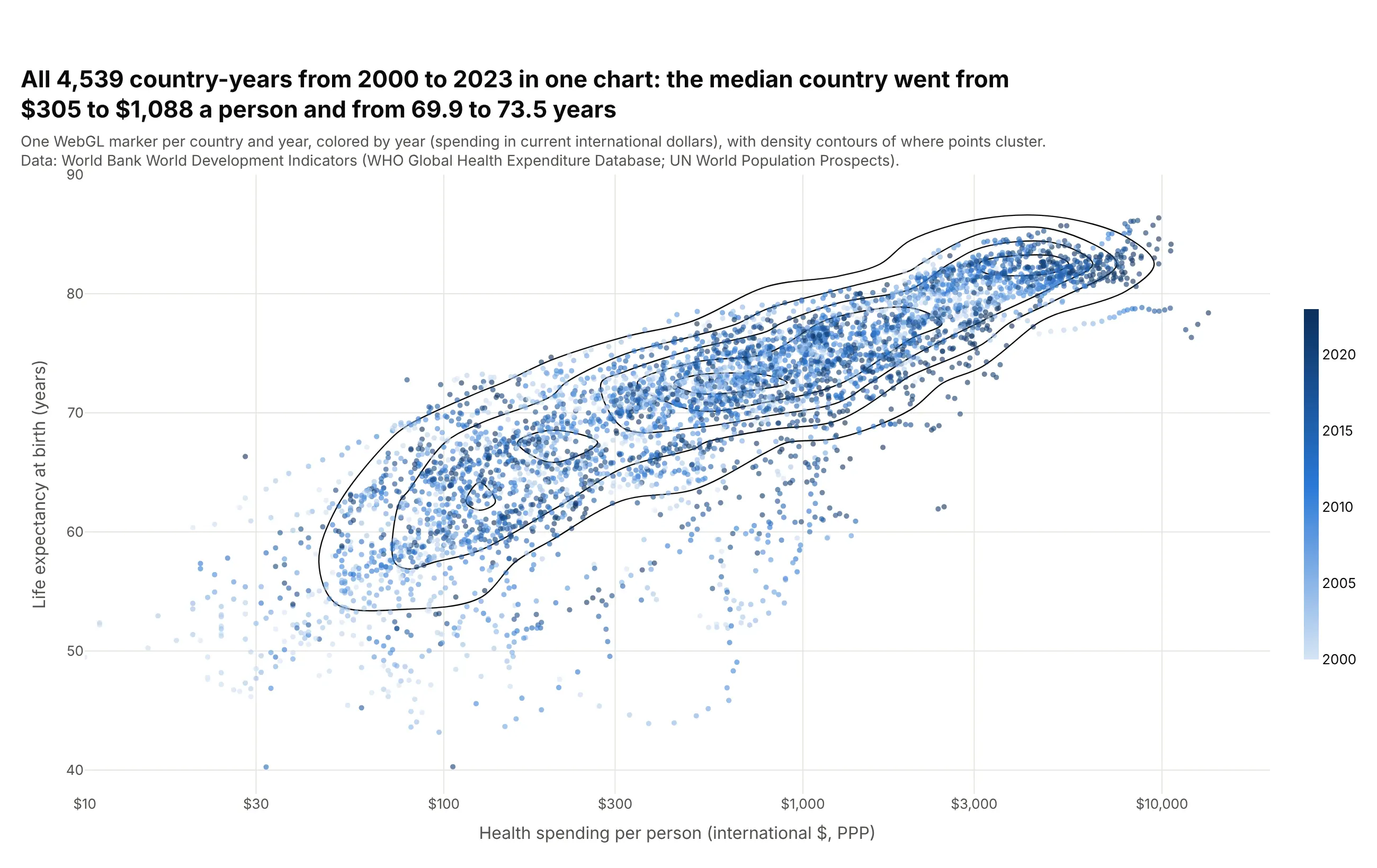
4,539 country-years from 2000 to 2023 drawn as small dots shaded from light blue in 2000 to dark blue in 2023 along the rising band, with black density contours outlining two dense clusters around $100 to $200 and $1,000 to $5,000

Drawing all 4,539 country-years at once with render_mode="webgl" keeps the chart fast, and density contours show where the points cluster when dots overlap. The median country went from $305 to $1,088 a person (in current dollars) and from 69.9 to 73.5 years, and the darker dots of later years sit up and to the right. Like histograms, plotly.js contours bin in linear units, so these are drawn on log10(spending) on a hidden axis laid over the log axis.

Prompt: Get the data from the World Bank World Development Indicators API (health spending per capita PPP and life expectancy, every country and year 2000-2023). Make a plotly scatter plot with px.scatter, render_mode="webgl", log_x=True, color="year" on a blue scale, and add a go.Histogram2dContour of log10(spending) and life expectancy with contours_coloring="none" on a hidden linear x axis overlaying the log axis.

12. 3D scatter plot

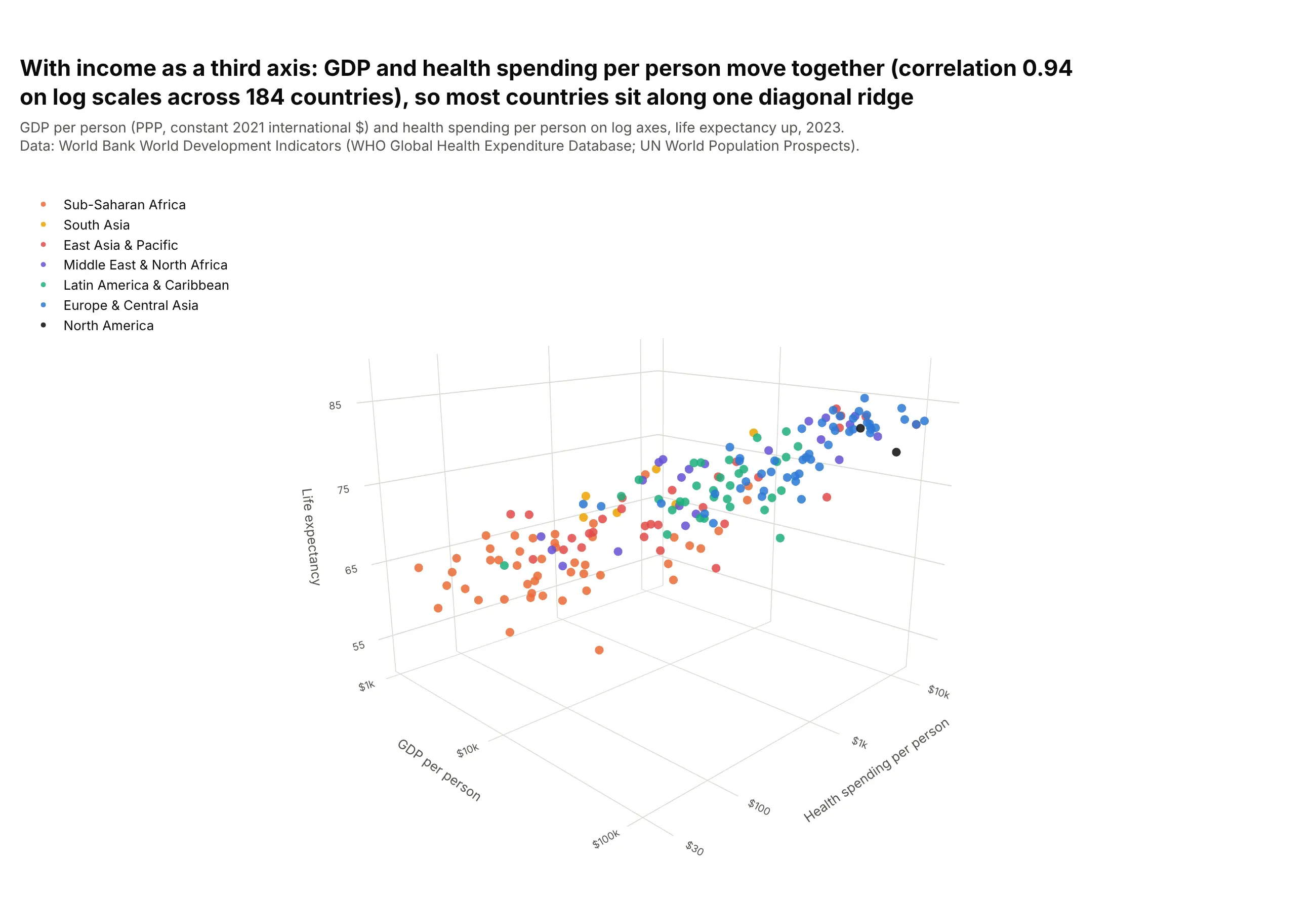
A 3D scatter plot of 184 countries with GDP per person and health spending per person on log axes along the floor and life expectancy up, colored by region, the dots forming one diagonal ridge from Sub-Saharan Africa at the low corner to Europe at the high corner

px.scatter_3d adds income per person as a third axis. GDP and health spending per person move together, with a correlation of 0.94 on log scales across 184 countries, so most countries sit along one diagonal ridge. A 3D scatter plot is best interactive, where you can rotate it; as a static image, the depth is hard to read, and a bubble chart or a color often shows the third number more clearly.

Prompt: Get the data from the World Bank World Development Indicators API: SH.XPD.CHEX.PP.CD, SP.DYN.LE00.IN and NY.GDP.PCAP.PP.KD (GDP per capita, PPP, constant 2021 international $) for 2023, with regions. Make a plotly 3D scatter plot with px.scatter_3d, x = log10(GDP per person), y = log10(health spending), z = life expectancy, color by region, dollar tick labels on the log axes, and a camera angle that shows the ridge.

13. Animated scatter plot

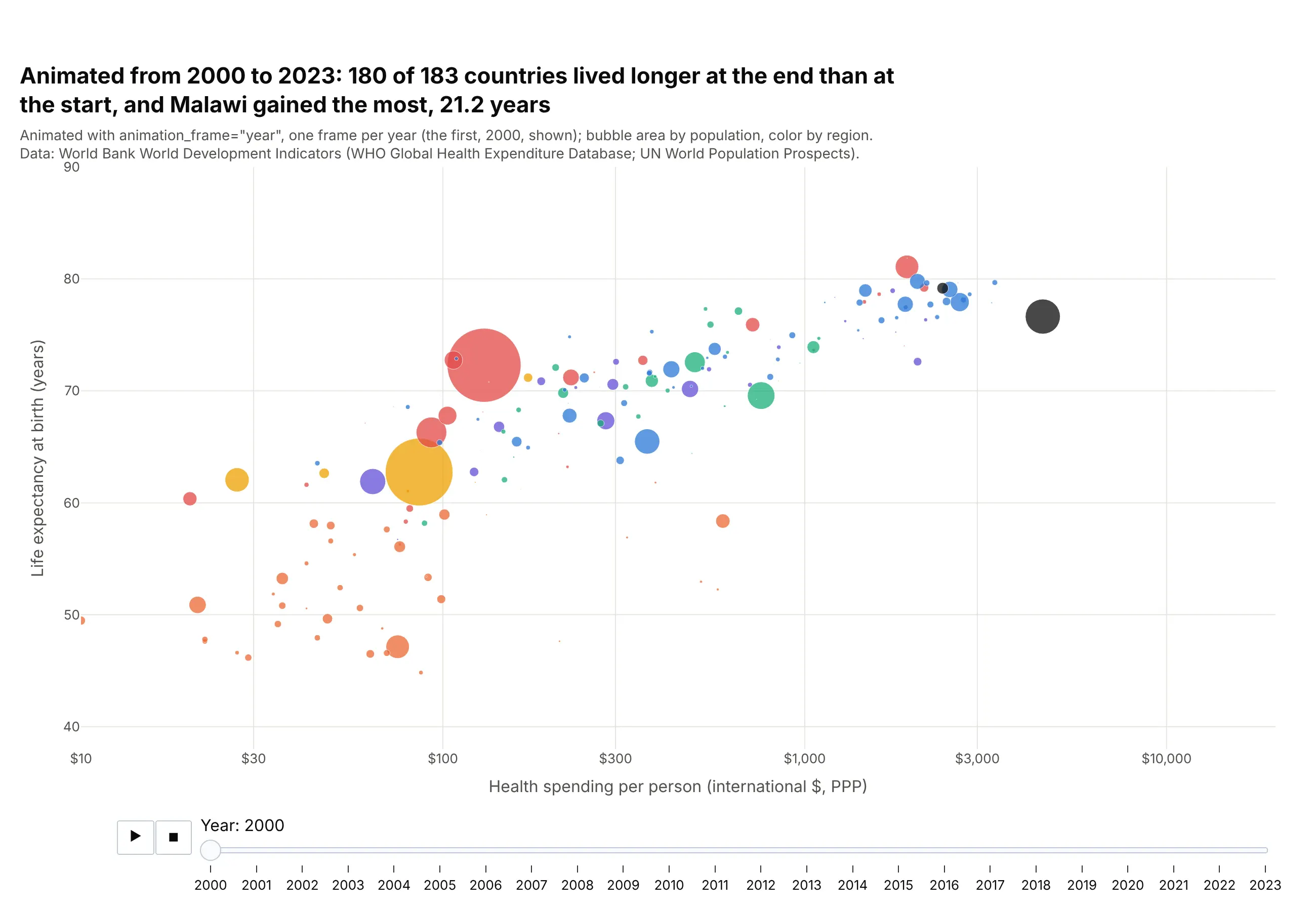
The bubble version of the chart at its first frame, 2000, with a play button and a year slider from 2000 to 2023 below it

animation_frame="year" with animation_group="country" adds play and pause buttons and a slider, and each country's bubble moves from year to year, as in Hans Rosling's Gapminder talks. Over the 24 frames, 180 of 183 countries lived longer at the end than at the start, and Malawi gained the most, 21.2 years. Fix range_x and range_y so the axes don't jump between frames. An animation can't be printed, so pair it with a static chart of the first and last year.

Prompt: Get the data from the World Bank World Development Indicators API (health spending per capita PPP, life expectancy, population, 2000-2023) with regions. Make an animated plotly bubble chart with px.scatter, animation_frame="year", animation_group="country", size="population", color by region, log_x=True, and fixed range_x=[10, 20000] and range_y=[38, 90].