Wind Rose Charts - A Complete Guide (with 14 Examples)

TL;DR

• A wind rose is a polar bar chart of how often the wind blows from each direction, with each bar split into speed bands. The same chart works for anything with a direction (waves, storm tracks, streets) or a cycle (hours of the day, months).
• Wind roses are also known as wind rose charts and polar bar charts, and are similar to radar charts and Nightingale rose charts.
• Use one when direction is the question: siting a wind turbine or a runway, finding where pollution comes from, or seeing when in the day something happens.
• Set north at the top and clockwise, match the number of sectors to how the data was recorded, and use a stacked bar chart instead when readers need to compare exact values.
• Any coding agent can make one with Plotly in a minute. In Python it's px.bar_polar(df, r="frequency", theta="direction", color="strength").

What is a wind rose?

Wind roses look like this:

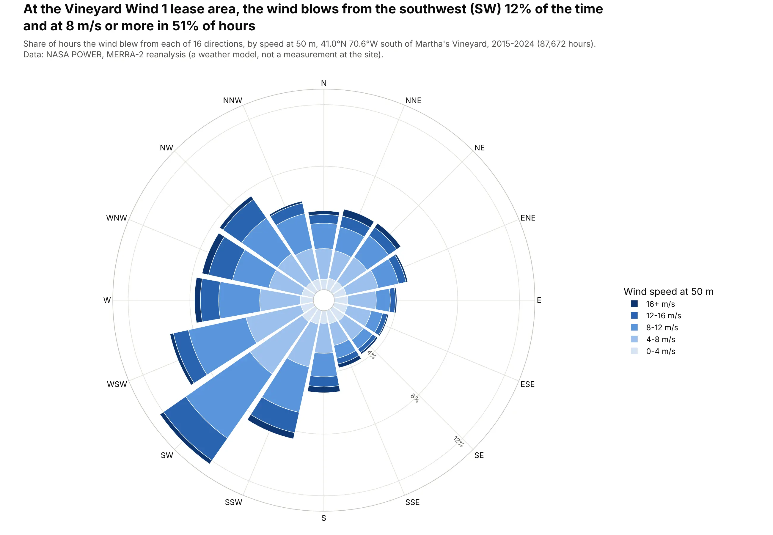
Data: NASA POWER, MERRA-2 reanalysis at 50 m (a weather model, not a measurement at the site), 2015-2024.

How do you read a wind rose? In the example above, notice these things:

• Each bar points to the compass direction the wind blew from, and its length is the share of hours it came from there. The southwest bar is the longest at 12% of hours, which makes southwest the prevailing wind at this site.
• North is at the top and the directions run clockwise like a compass. The long bars from SSW to WSW sit side by side, so the prevailing wind covers a broad arc around the southwest, and the short bars on the southeast side show that wind from there is rare.
• The shades of blue split each bar by wind speed, from the lightest near the center for the slowest winds to the darkest at the tip for the fastest. More than half of the southwest bar is in the three darker bands, 8 m/s or faster, so the most common wind is also a strong one, which is what a wind farm developer wants to see.
• The gray rings mark the share of hours and are labeled along the southeast spoke. Each bar is measured from the small circle in the middle, so you read its length against the rings to get its share.
• The bars show where the wind comes from, so the southwest bar means wind blowing toward the northeast. Because each wedge gets wider as it goes out, the outer bands also look bigger than inner bands of the same length, so compare how far each band reaches along its spoke.

It's often used for charts like these:

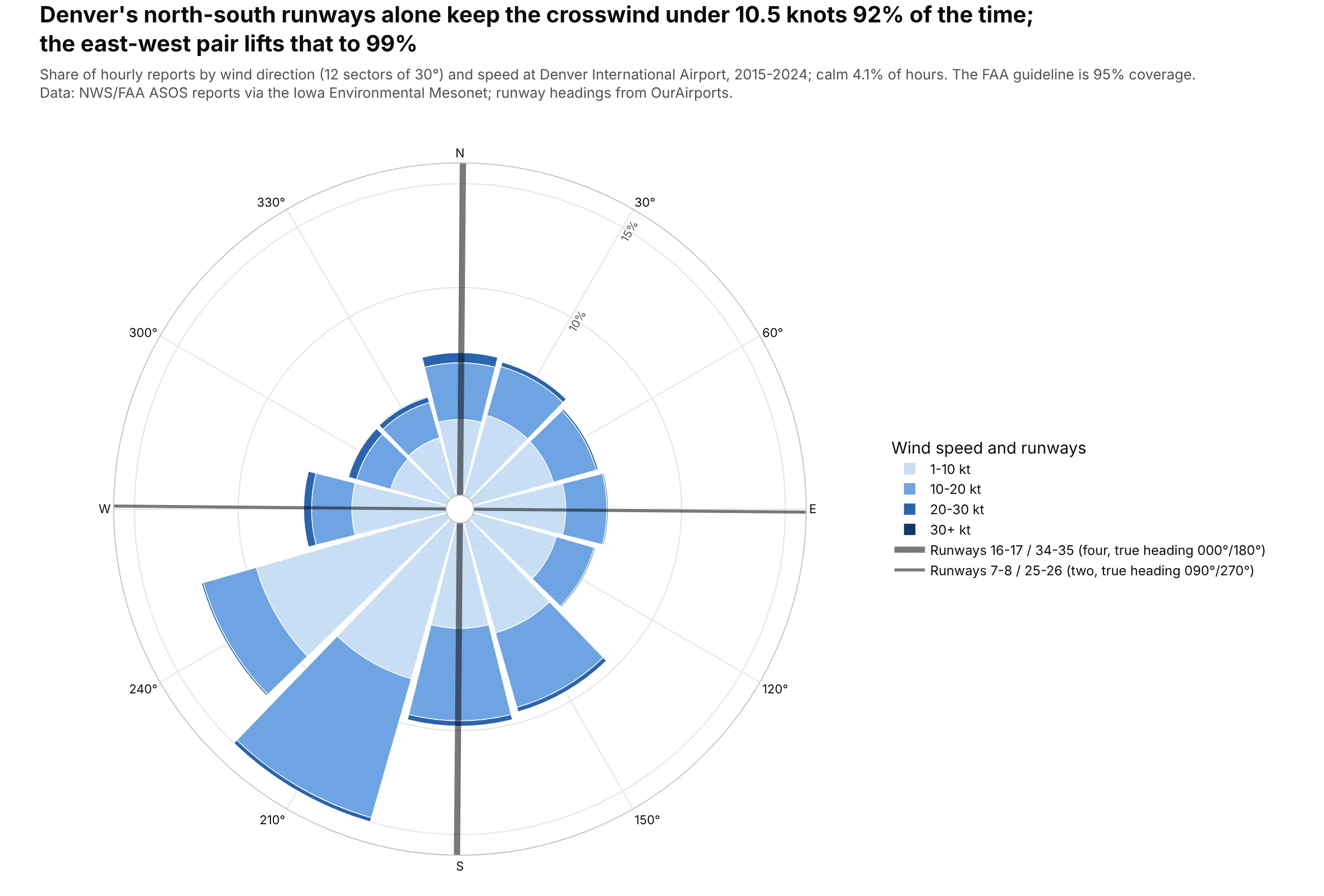
Laying out an airport. Denver's four north-south runways alone keep the crosswind under 10.5 knots in 92% of hours, and its two east-west runways lift that to 99%, above the FAA's 95% guideline. Data: NWS/FAA ASOS reports via the Iowa Environmental Mesonet, 2015-2024; runway headings from OurAirports.

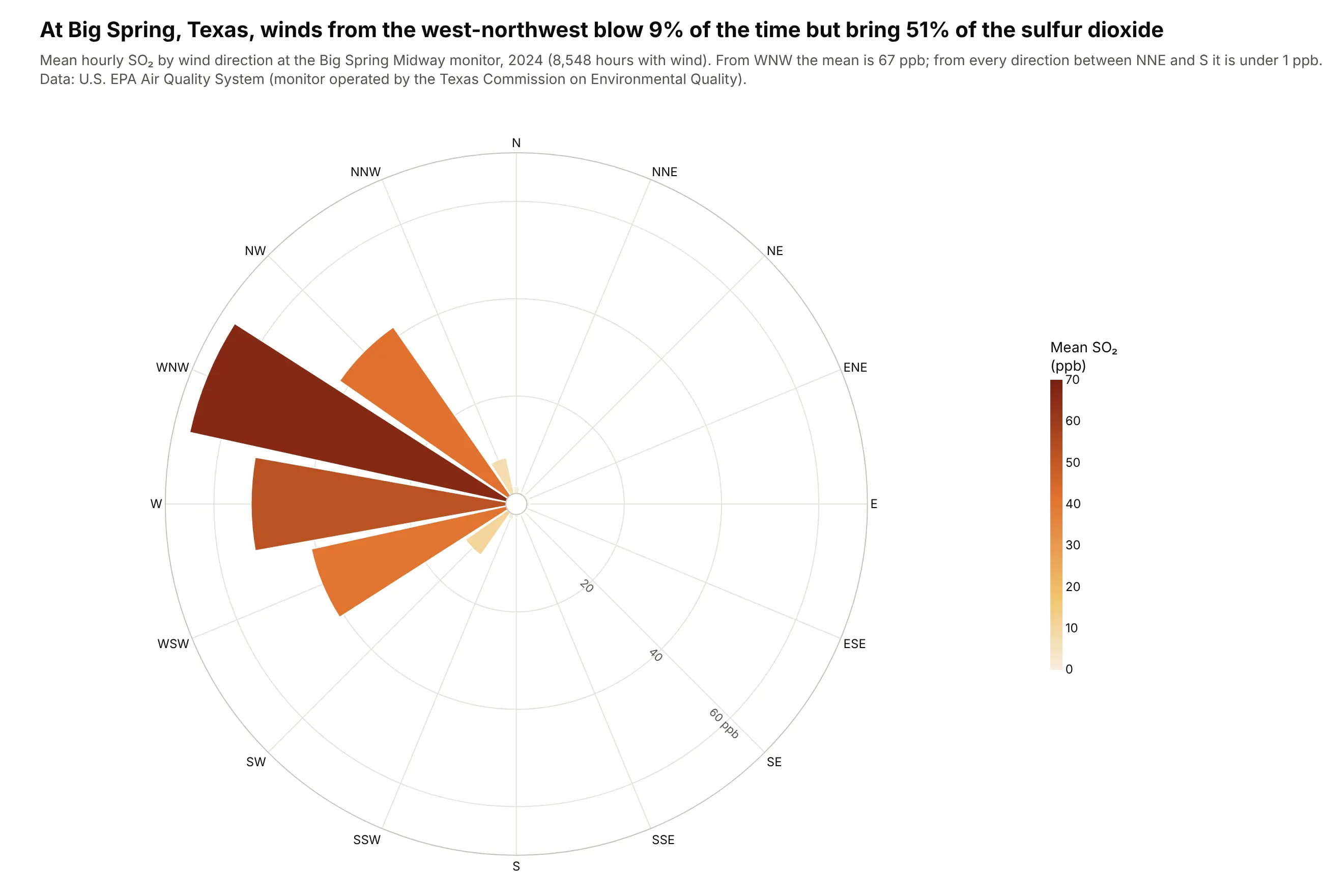
Finding where pollution comes from. With bar length set to the mean concentration instead of the share of hours, the rose points at the source: wind from the west-northwest blew 9% of the time at this Texas monitor but brought 51% of its sulfur dioxide. Data: U.S. EPA Air Quality System, 2024.

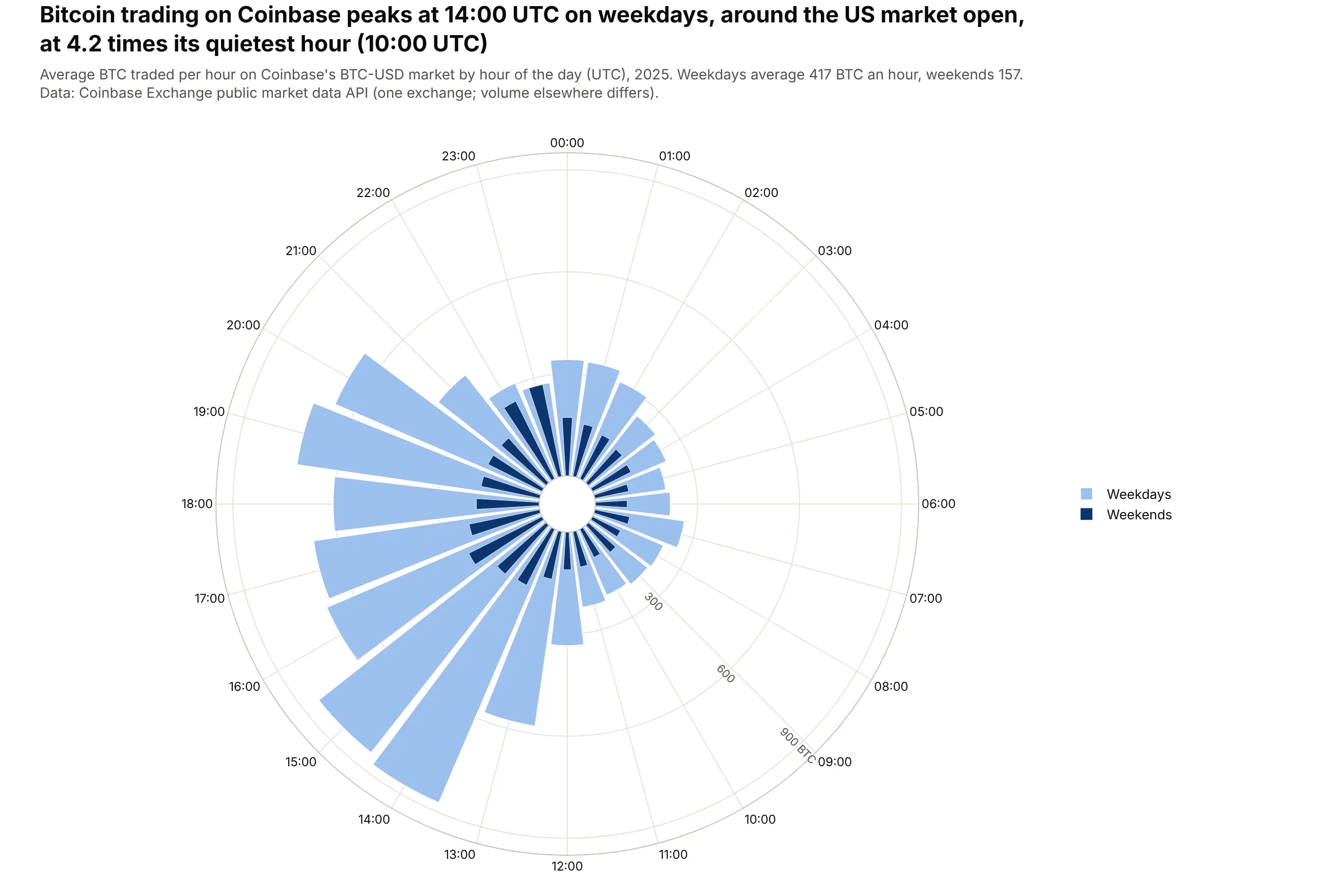
A 24-hour clock. Weekday bitcoin trading on Coinbase peaks at 14:00 UTC, around the US market open, at 4.2 times its quietest hour, and weekends average 157 BTC an hour against 417 on weekdays. Data: Coinbase Exchange public API, BTC-USD hourly candles, 2025.

A short history

Compass roses on maps are centuries old, but the best-known early polar bar chart of data is Florence Nightingale's diagram of deaths in the British Army during the Crimean War, published in 1858. Each wedge is a month and its area is the death rate, which showed that disease killed far more soldiers than wounds: 84% of the deaths from April 1854 to March 1855. Lee Brasseur analyzes the diagrams in Technical Communication Quarterly (2005). Here is her chart redrawn from her data:

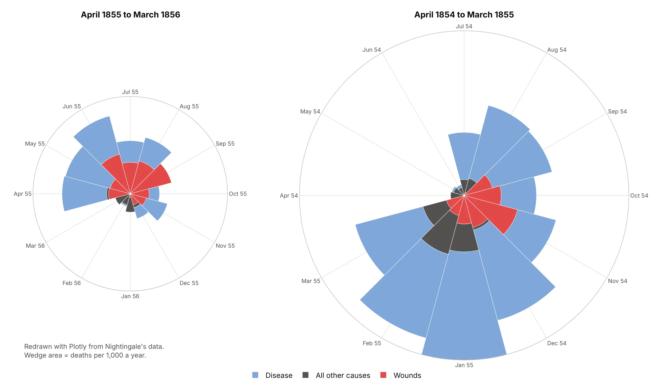
Nightingale made the wedge area proportional to the rate, so the redraw plots the square root of each rate. Meteorologists use the same layout for wind, and the FAA's airport design guidance (Advisory Circular 150/5300-13B) uses a wind rose to check how well runways line up with the wind.

Alternatives to a wind rose

Here's the same Vineyard Wind direction and speed table drawn five ways. Some are better for the question, some worse, some just different:

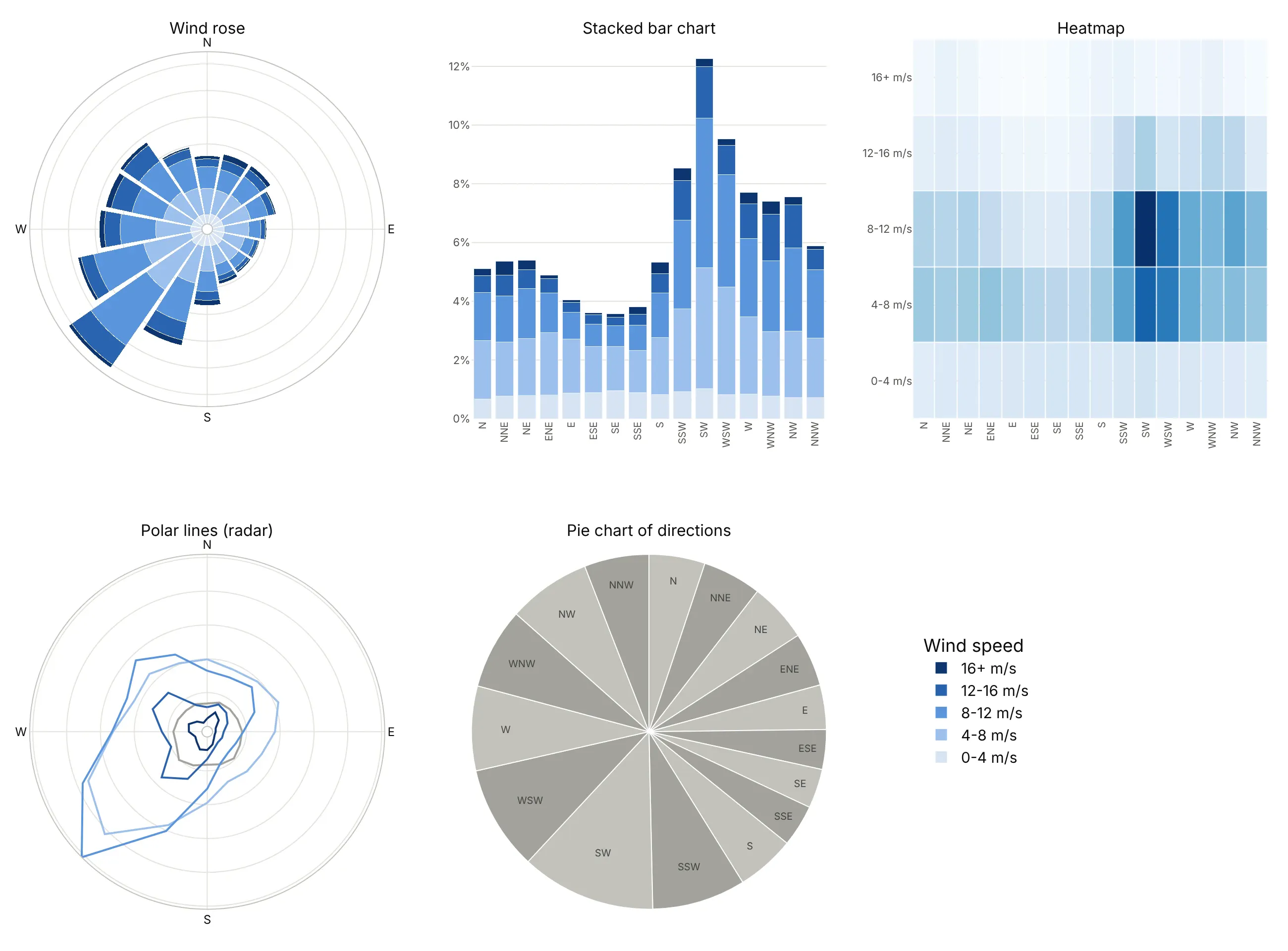
• Stacked bar chart (better for precise comparisons). Bars on a shared baseline are easier to compare than wedges, and you can read that southwest (12.3%) is more than three times southeast (3.6%). You lose the compass, so north and north-northwest end up at opposite ends of the axis.
• Heatmap (different). Shows each direction and speed band as its own cell, which makes the most common combination (southwest at 8-12 m/s) stand out, but the totals per direction disappear. See our heatmap guide.
• Polar lines (worse). One line per speed band, as in a radar chart, keeps the compass, but the lines cross and readers can't add them up in their heads. See our radar chart guide for when the radar layout fits.
• Pie chart (worse). Slices are ordered like a compass, but each slice's angle is its share, so the slices no longer point in their own direction and the speed bands are gone.

How to make a wind rose

With AI

ChatGPT, Claude Code, GitHub Copilot, Cursor and other AI tools are excellent at writing Plotly code. Name Plotly in the prompt, say how to bin the directions and speeds, and list the checks you want:

With Plotly Studio

Plotly Studio is a desktop app where you point an AI at a dataset and it builds charts and a Dash app around your questions. Ask for a wind rose the same way:

Show a wind rose of this file with 16 directions stacked by wind speed, north at the top. Add a dropdown to pick the month and print the calm share in the middle.

Make a wind rose or polar bar chart in Python or JavaScript

This is the code AI tools write under the hood. A wind rose is one of Plotly's polar charts, and in Python, Plotly Express takes one row per direction and speed band:

To bin raw observations yourself, cut the directions into sectors and the speeds into bands with pandas, then add one go.Barpolar trace per band:

In JavaScript, plotly.js takes one barpolar trace per speed band:

Without rotation: 90 and direction: "clockwise", numeric angles follow math convention (0 at the right, counterclockwise), so a wind rose comes out mirrored. The same polar axes also draw polar scatter and polar line charts with go.Scatterpolar (scatterpolar in JavaScript), with mode set to markers, lines or both.

Share it

Every Plotly chart has a Share chart button (the cloud icon in its toolbar) that uploads it to Plotly Cloud and gives you a link. Only you can see it until you change its visibility.

For a live app, put the chart in a Dash app and publish it with the Plotly Cloud CLI. Coding agents can run these commands for you:

If your data has to stay in your own cloud or data center, publish to Dash Enterprise instead.

Dos and don'ts

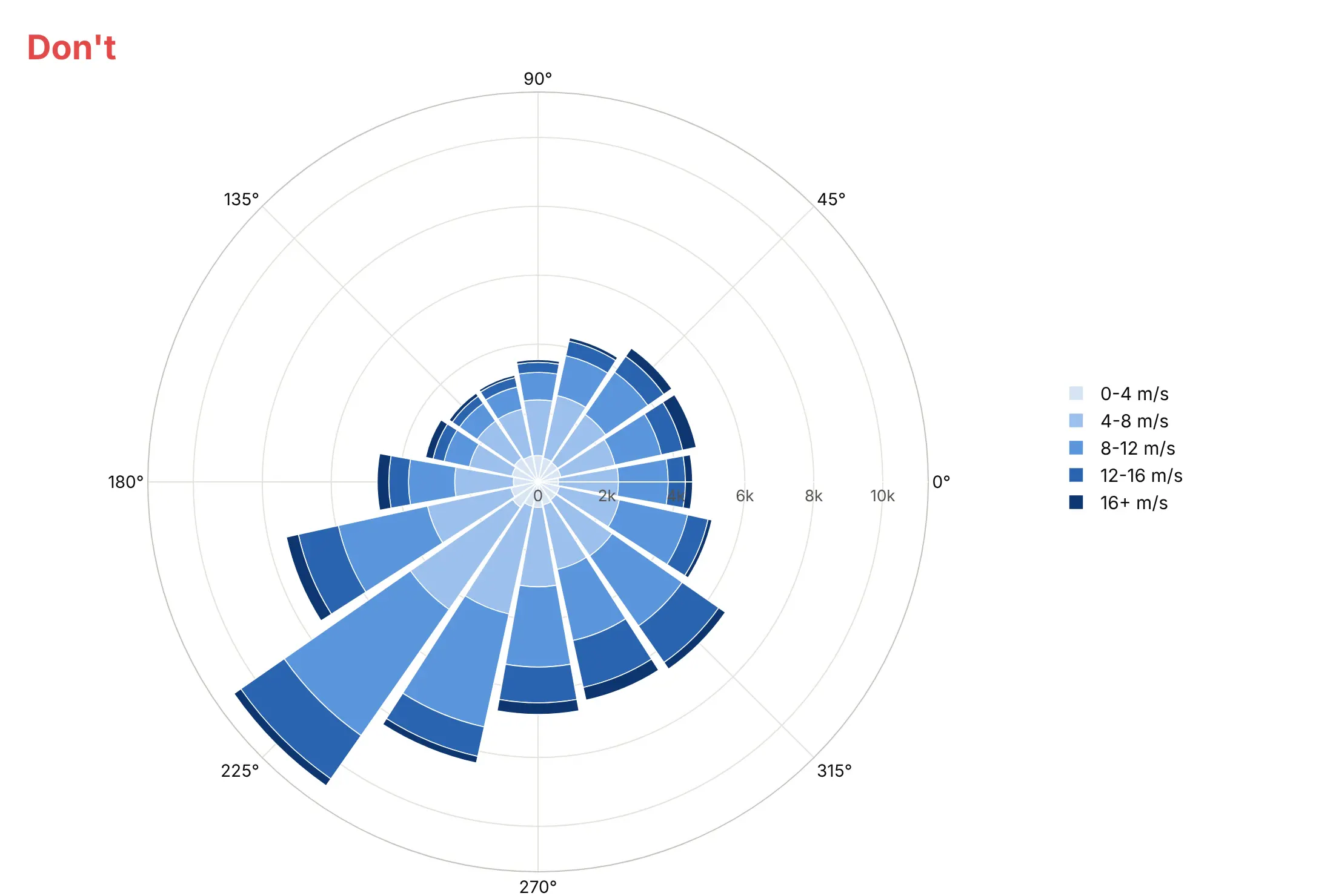
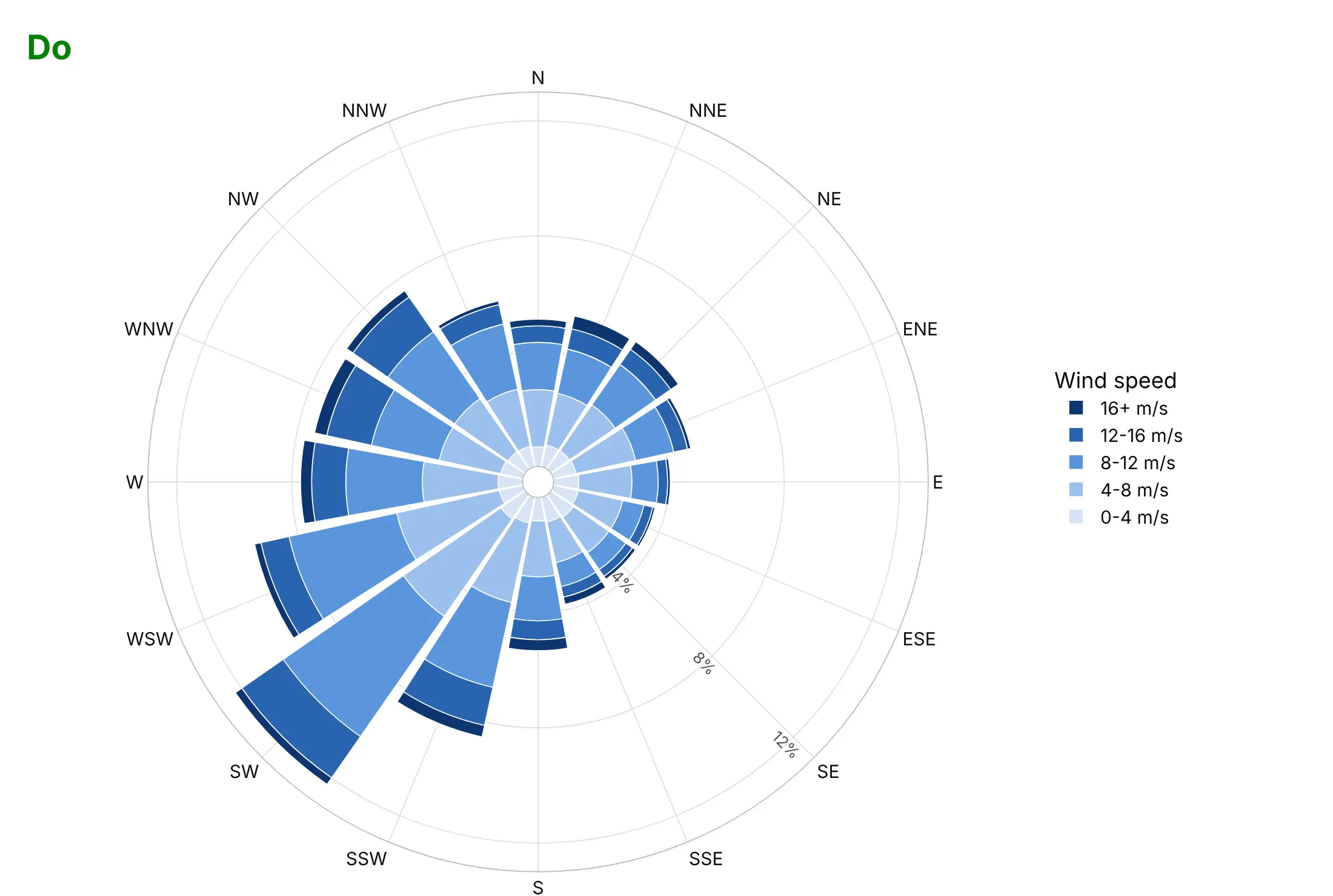
Most wind rose mistakes come from the angles, because Plotly's polar axes start with math conventions. Here is the same Vineyard Wind data both ways, with the same colors.

Don't pass directions as numbers without setting the rotation and direction, show raw hour counts, or let the radial tick labels sit on the bars. Here west winds are drawn at the bottom, where south belongs, and the legend lists the speed bands in the opposite order of the stack:

Do put north at the top and go clockwise, label the compass points, show shares of time in %, move the radial ticks to an empty sector and reverse the legend so it matches the stack:

Match the sectors to how the data was recorded

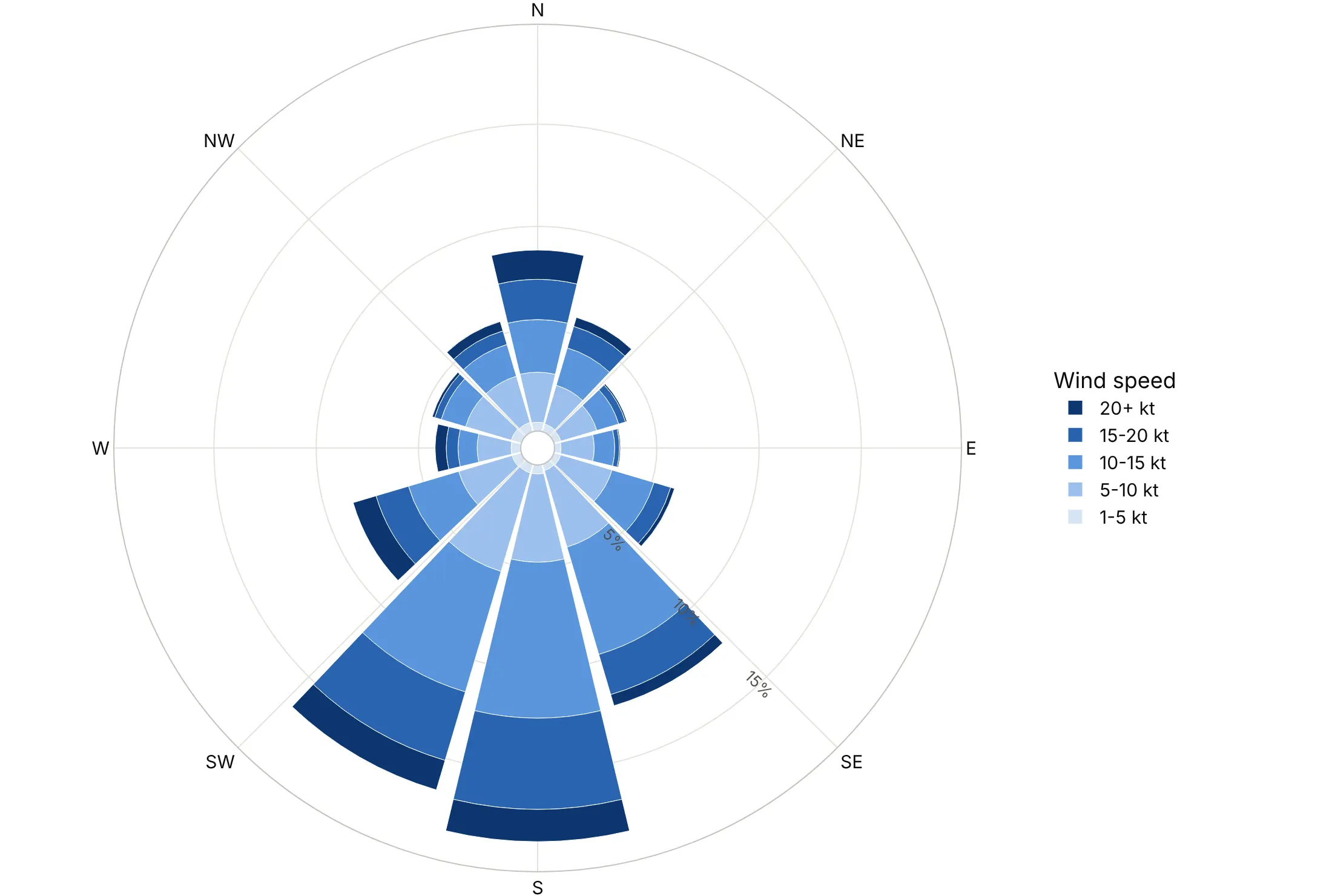
Airport weather reports (METAR) give the wind direction in whole tens of degrees, so the number of sectors changes the shape of the rose. Here is Amarillo's wind binned three ways.

36 sectors of 10 degrees. One sector per reported value, so nothing is aliased. Amarillo's south and south-southwest winds are all close to 6.4% of hours.

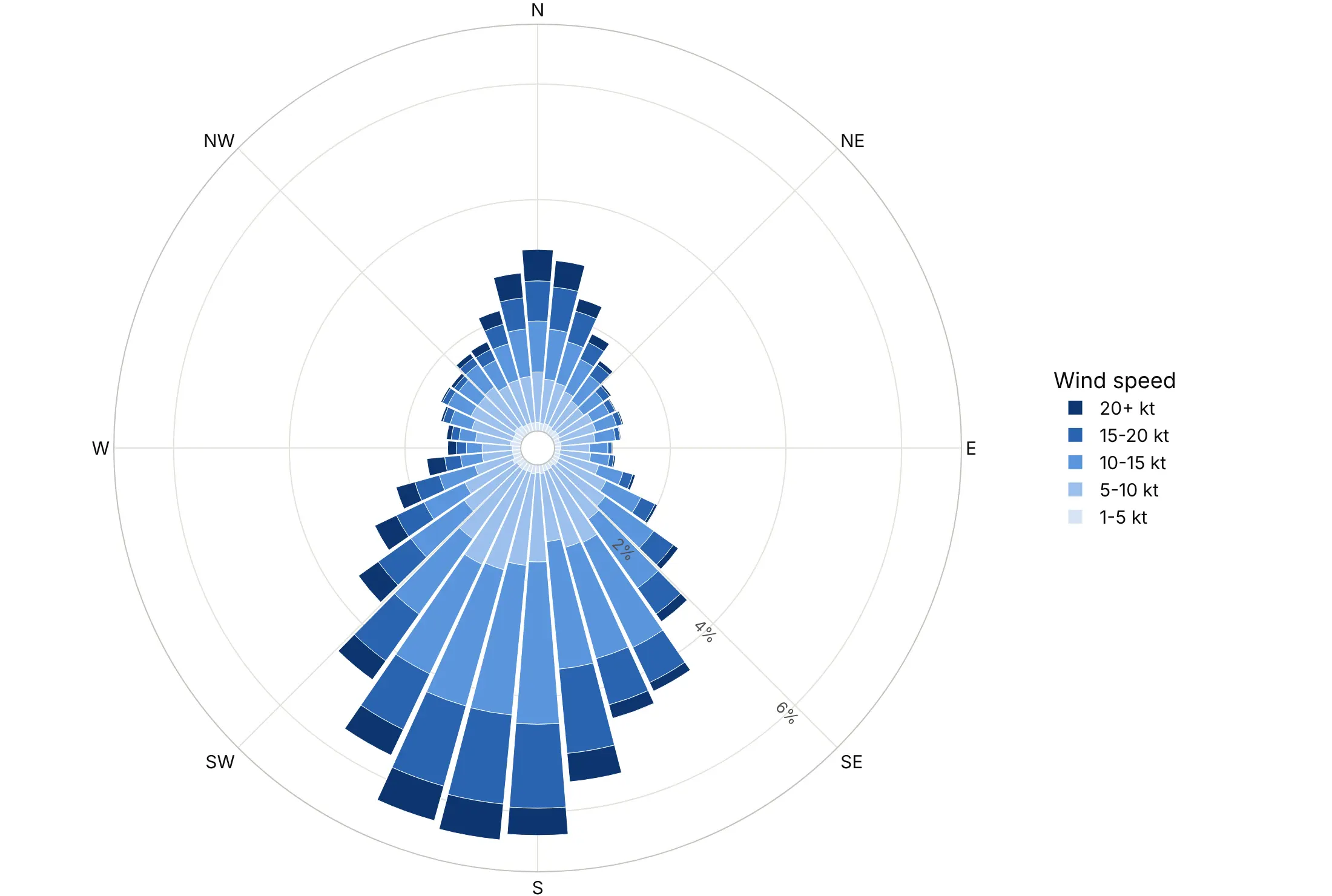
16 sectors (avoid for METAR data). The north, east, south and west sectors each hold three reported values and the other 12 hold two, so south (18.4%) looks half again as big as south-southwest (12.0%) even though the underlying values are the same.

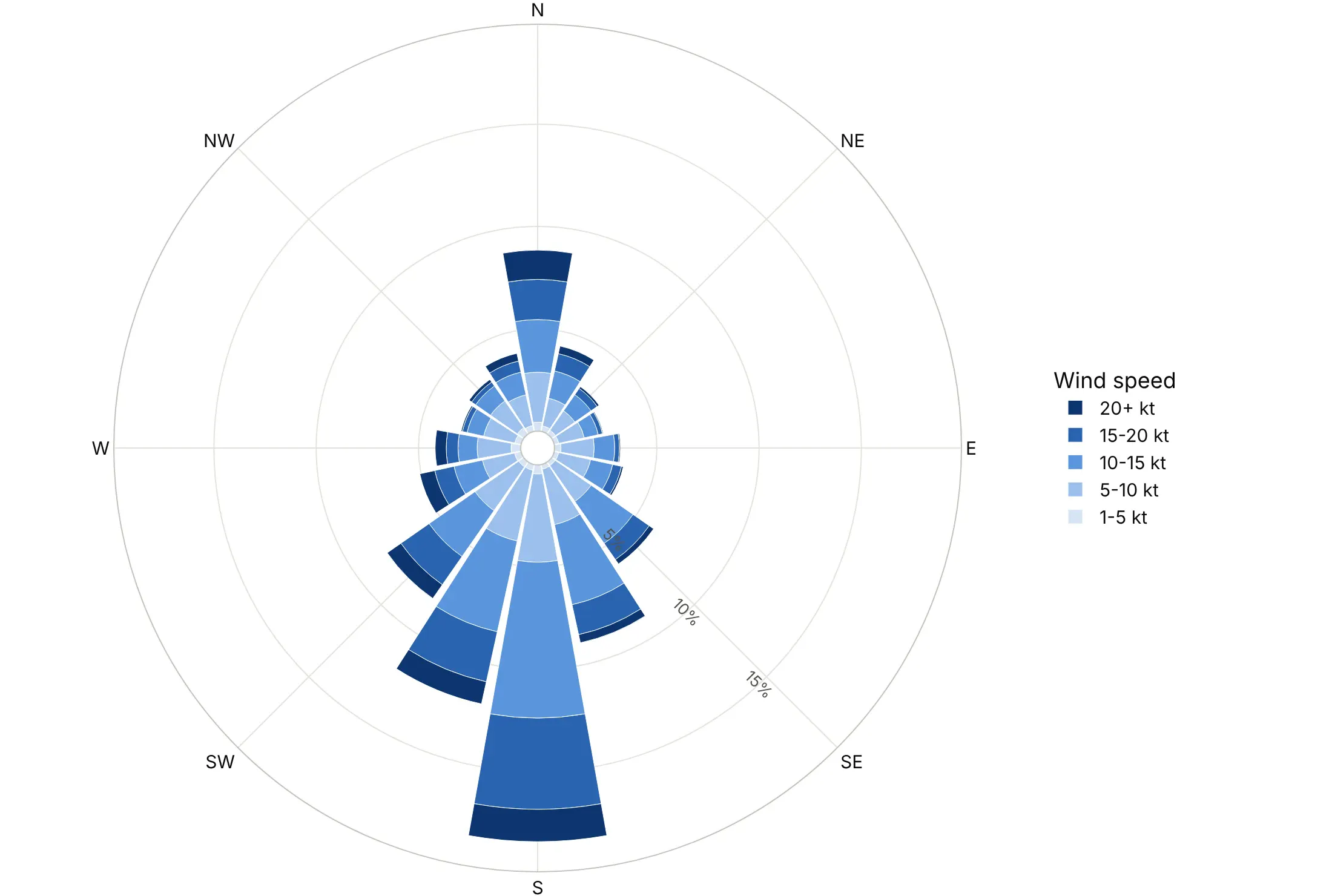
12 sectors of 30 degrees. Each sector holds exactly three reported values, so the rose is smooth again with fewer, wider bars.

Checklist

Do

• Set angularaxis.rotation=90 and direction="clockwise" for anything on a compass.
• Say whether bars show where the wind comes from (meteorology) or where something goes (storms, currents).
• Show shares of time in %, and print the calm share separately.
• Use a light-to-dark sequence for ordered bands like speed, and reverse the legend with traceorder="reversed" so it reads like the stack.
• Use the same radial range for roses you compare.

Don't

• Use 16 sectors for data recorded in 10-degree steps.
• Map a value to the radius when the chart should compare areas; plot the square root, as Nightingale did.
• Put a second quantity with different units on the same radial axis.
• Use a rainbow of colors for speed bands, which have a natural order.

Options to customize

These are the go.Barpolar (and px.bar_polar) options and the layout.polar settings that matter most. The full list is in the Plotly polar chart documentation and the wind rose documentation.

1. r, theta: the bar length and its angle, as compass labels (categories) or degrees.
2. color (px only): the column that splits each bar into stacked bands.
3. width: the angular width of each bar in degrees, for numeric theta such as 36 sectors of 10.
4. base: where bars start, for bars that grow inward and outward from a reference circle (example 3).
5. marker.color, marker.colorscale: one color per trace, or a continuous scale with a colorbar (example 7).
6. marker.line: a thin white outline that separates stacked bands.
7. polar.barmode: stack for a wind rose, overlay to draw one series inside another.
8. polar.bargap: the gap between bars; 0 for a histogram look.
9. polar.angularaxis.rotation, direction: 90 and clockwise for a compass or a clock.
10. polar.angularaxis.categoryarray, tickvals, ticktext: the order of categories and which labels to show.
11. polar.radialaxis.range, tickvals, ticksuffix: a fixed scale for comparisons and tick labels in %.
12. polar.radialaxis.angle: the angle of the radial ticks, in the polar's own frame; move them to an empty sector.
13. polar.hole: an empty center, for a calm share or a label.
14. polar.sector: draw only part of the circle, such as [45, 135] for a baseball field (example 10).
15. polar.domain: place several roses side by side.
16. legend.traceorder: reversed makes the legend match the stack.

More wind rose examples

Ten more polar bar charts built from real public data, each with its source, the technique that makes it work and a prompt to rebuild it.

1. Where the energy in the wind comes from

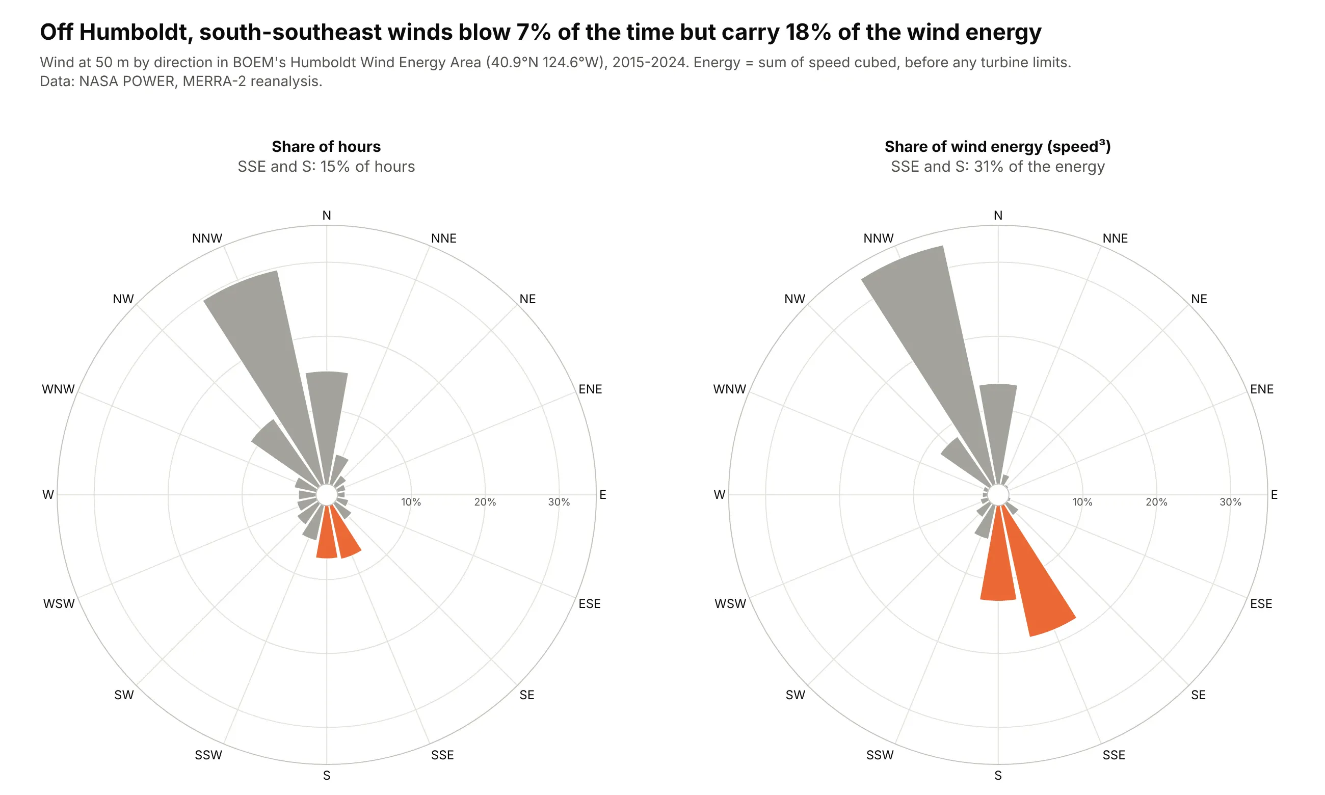
Off Humboldt, California, the wind blows mostly from the north-northwest, but south-southeast winds are 7% of hours and 18% of the energy in the wind. Energy goes with the cube of speed, so a frequency rose undersells the fast directions. Data: NASA POWER, MERRA-2 reanalysis at 50 m, 2015-2024.

Tip: two go.Barpolar traces in polar and polar2 with the same radialaxis.range make the two roses directly comparable.

2. Wind farm wakes, turbine by turbine

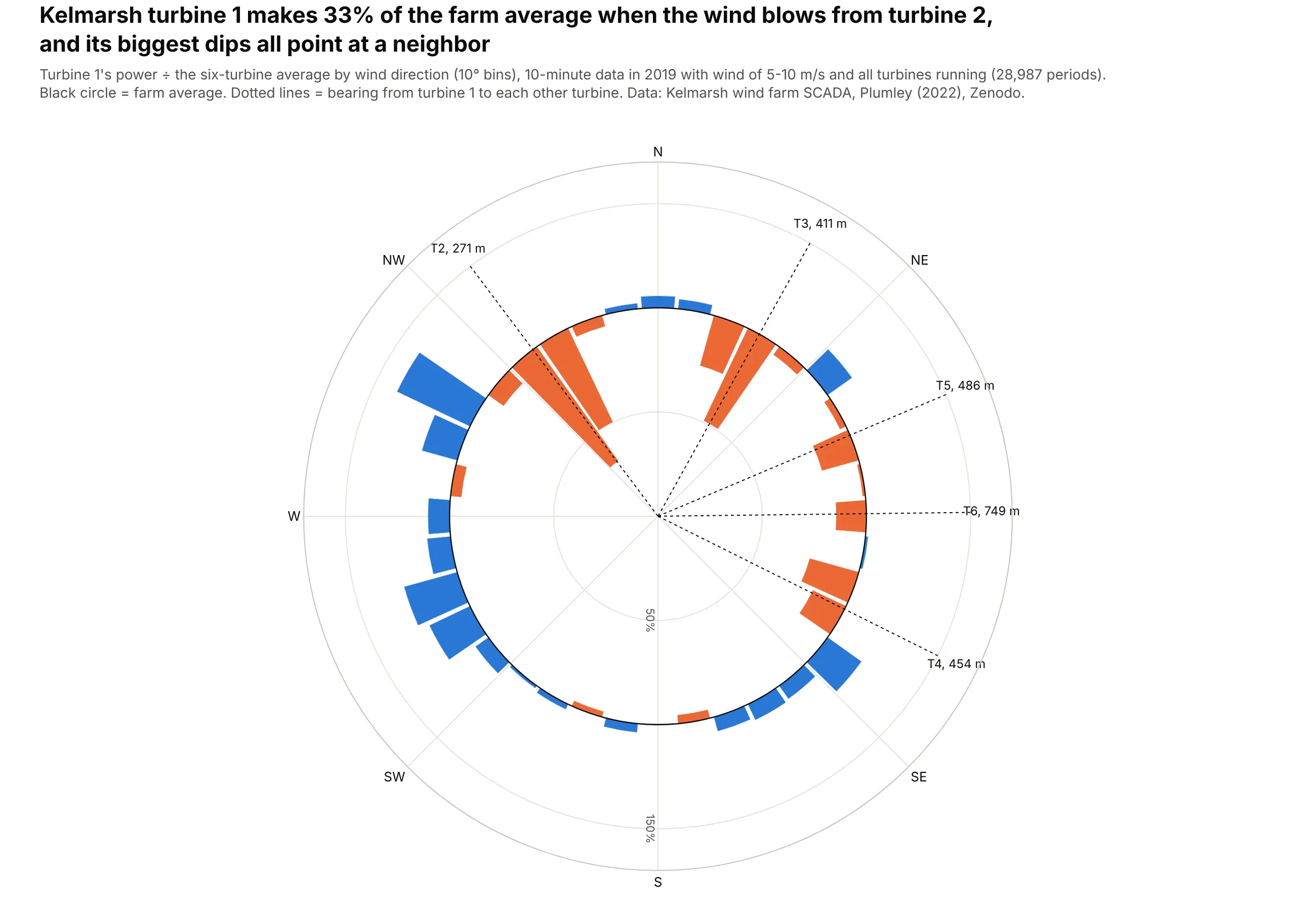
When the wind blows from turbine 2, 271 m away, turbine 1 makes 33% of the farm's average output, and each of its other dips lines up with a neighbor. This is wake loss, the reason turbines are spaced apart in the prevailing wind direction. Data: Kelmarsh wind farm SCADA data, 2019, Plumley (2022), Zenodo.

Tip: go.Barpolar(r=ratio - 1, base=1) makes bars start at the farm-average circle, so losses point inward and gains outward.

3. A windy airport and a calm one

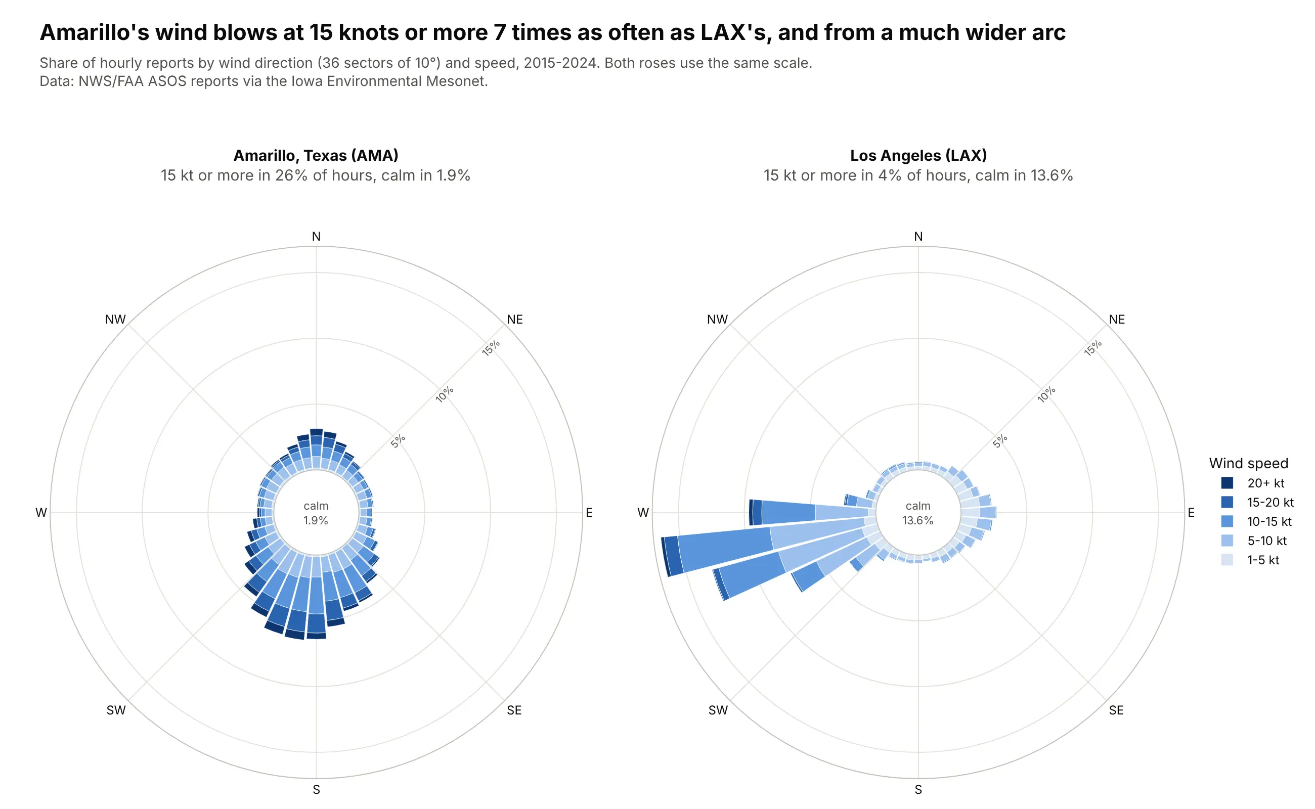
Amarillo's wind blows at 15 knots or more in 26% of hours against 4% at LAX, and LAX is calm 13.6% of the time. LAX's wind also comes from a narrow arc: three 10-degree sectors from 250 to 270 degrees hold 39% of hours. Data: NWS/FAA ASOS reports via the Iowa Environmental Mesonet, 2015-2024.

Tip: with polar.hole, the empty center has room for the calm share, which has no direction and so no bar.

4. Waves on Oahu's North Shore, winter vs summer

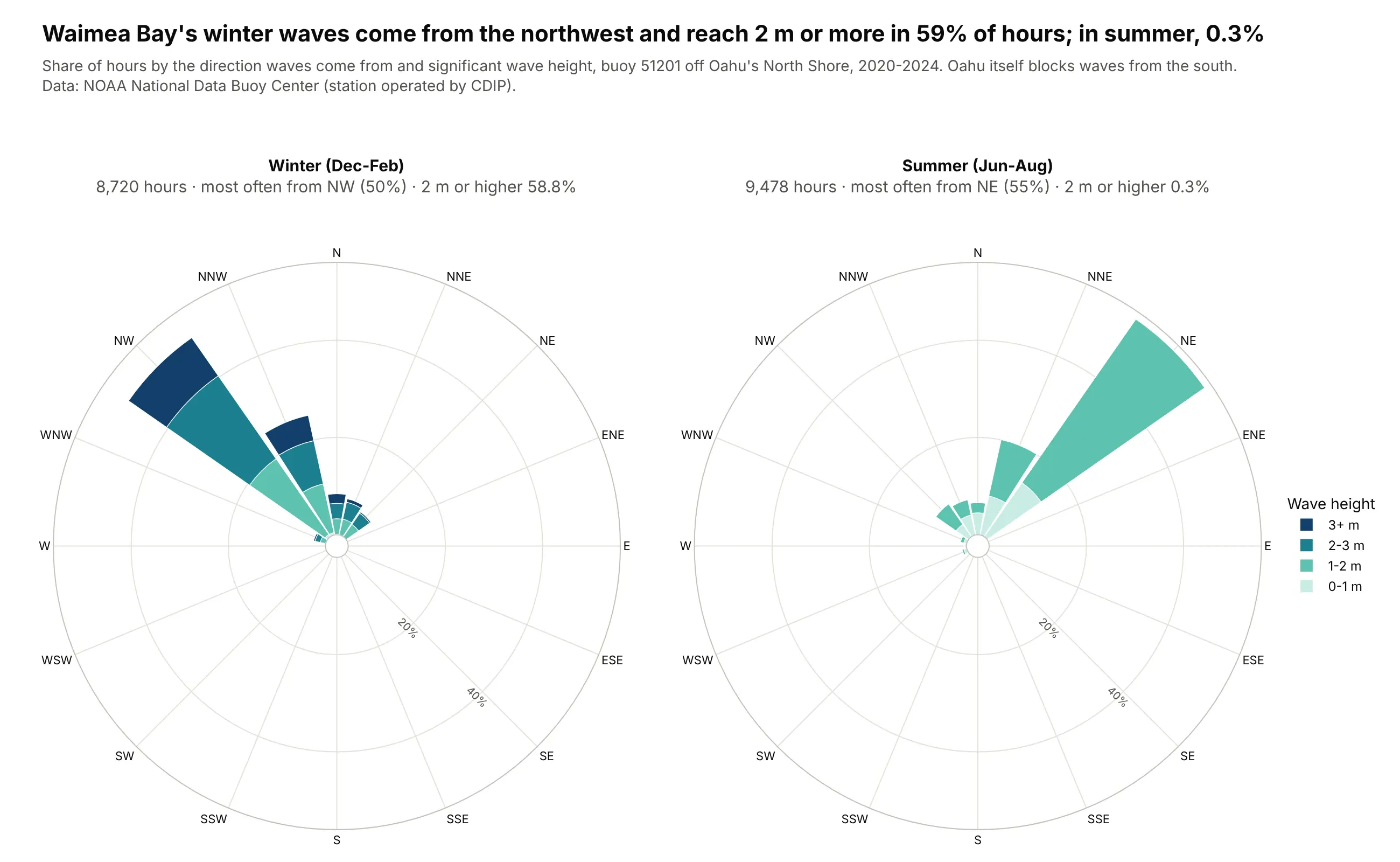
The same chart works for waves: in winter, half of Waimea Bay's waves come from the northwest and 59% of hours have waves of 2 m or more, while in summer the waves come from the northeast and reach 2 m in 0.3% of hours. Data: NOAA National Data Buoy Center, station 51201, 2020-2024.

Tip: pick a color sequence that fits the subject (teal to navy for the sea) but keep it light to dark for ordered bands.

5. Natural gas use by month, 2005 vs 2025

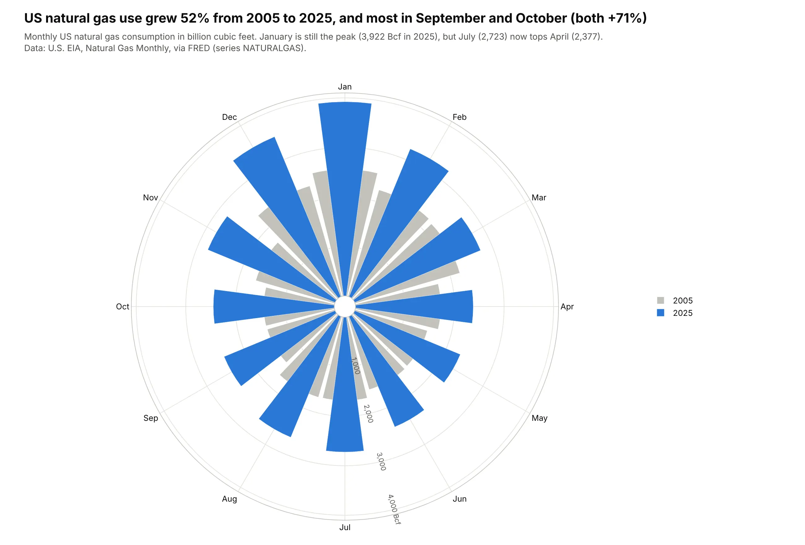
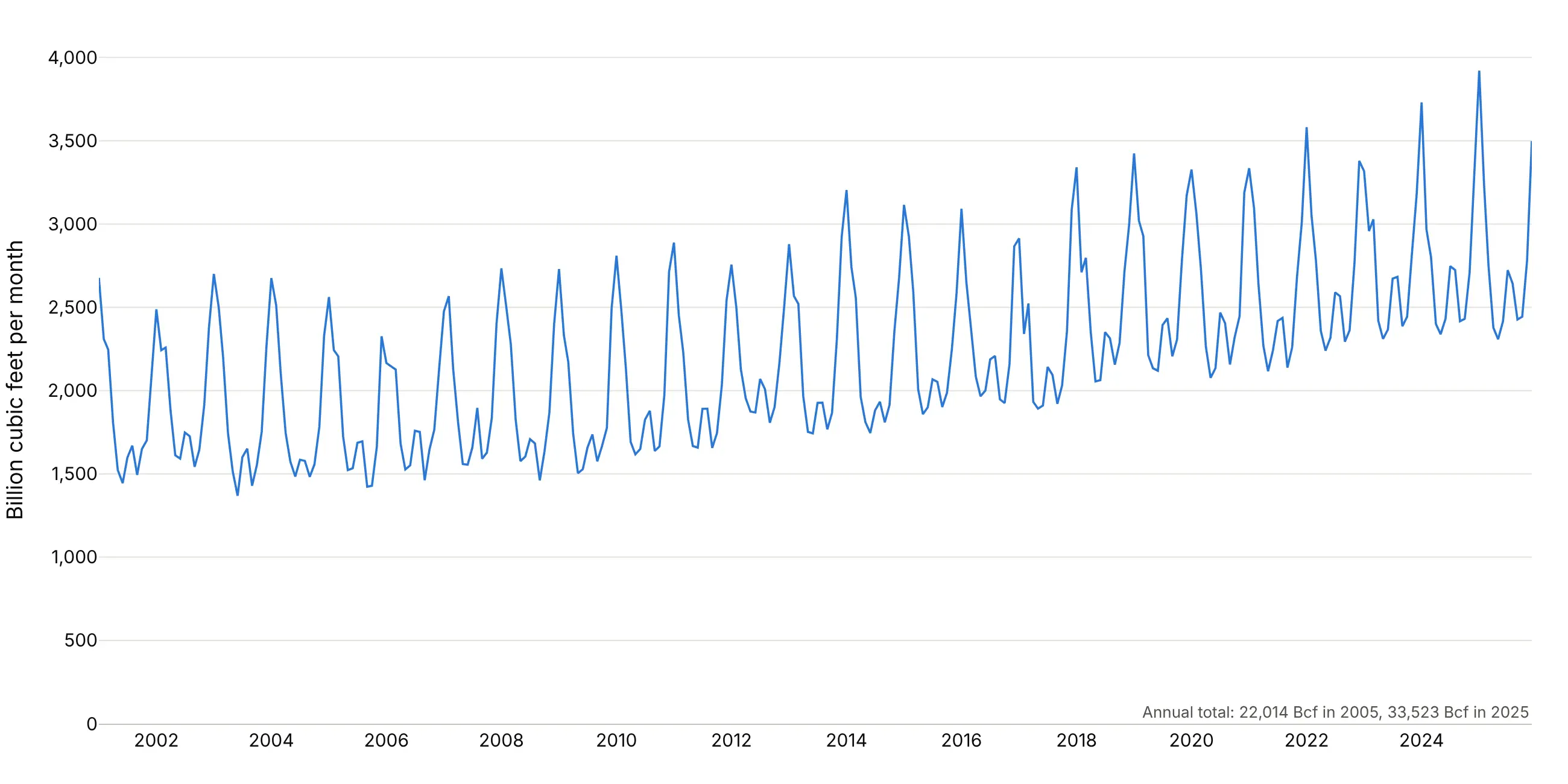
US natural gas use grew 52% from 2005 to 2025, and the growth was largest in September and October (both +71%). On a 12-month clock the winter peak stays in one piece at the top. Data: U.S. EIA, Natural Gas Monthly, via FRED (series NATURALGAS).

Tip: polar.barmode="overlay" with a wide gray trace and a narrow colored one shows two years in the same wedge.

Another way to see it: a line of every month since 2001 shows the growth and the seasons together, and makes it clear that the rise is steady rather than a jump between two years.

6. The flu season as a clock

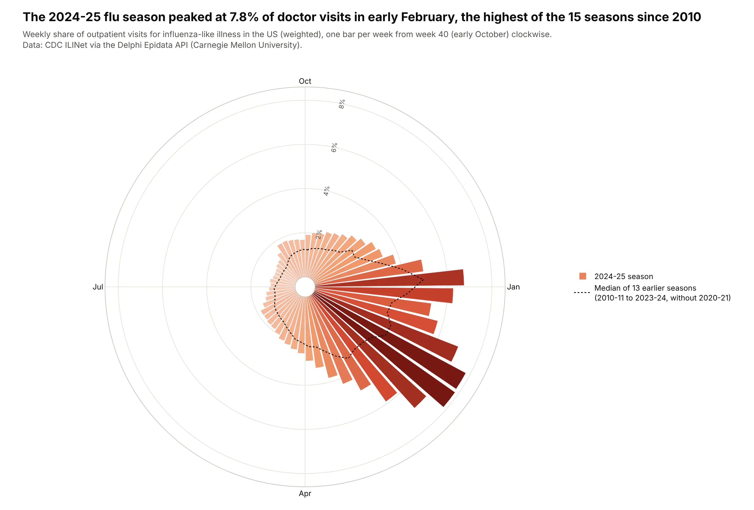
The 2024-25 flu season peaked at 7.8% of doctor visits in early February, the highest of the 15 seasons since 2010-11. Starting the clock in October keeps each season in one piece, and the dotted line shows a typical season. Data: CDC ILINet via the Delphi Epidata API.

Tip: with numeric theta (week x 360 / 52) and a width of one week, 52 bars fit around the circle, and month labels go in tickvals and ticktext.

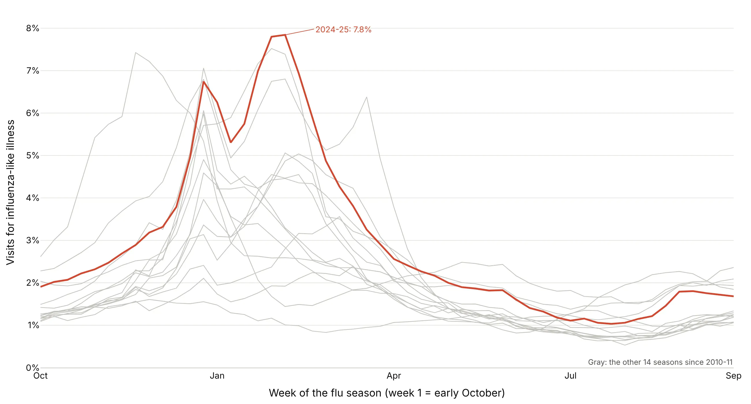
Another way to see it: all 15 seasons as lines show that 2024-25's peak was the highest, and that 2022-23 peaked in late November instead.

7. When New Yorkers call 311

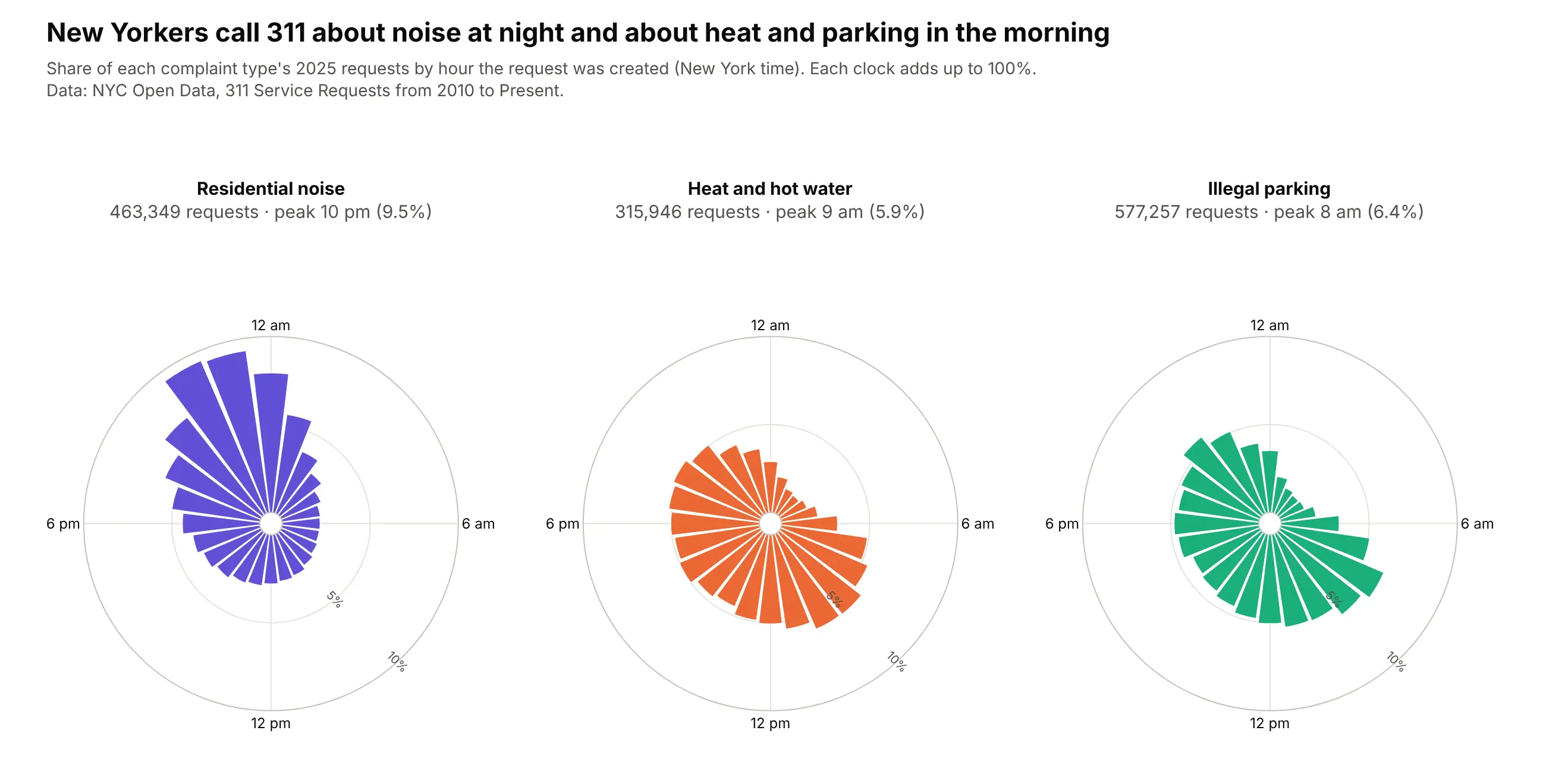
Residential noise complaints peak at 10 pm, with 32% of them between 10 pm and 2 am, while heat and illegal parking complaints peak at 9 am and 8 am. Each clock is normalized to 100%, so the shapes compare even though parking had 577,257 requests and heat 315,946. Data: NYC Open Data, 311 Service Requests, 2025.

Tip: aggregate on the server with SoQL's date_extract_hh(created_date) so you download 72 rows instead of 1.36 million.

8. Where Atlantic hurricanes go

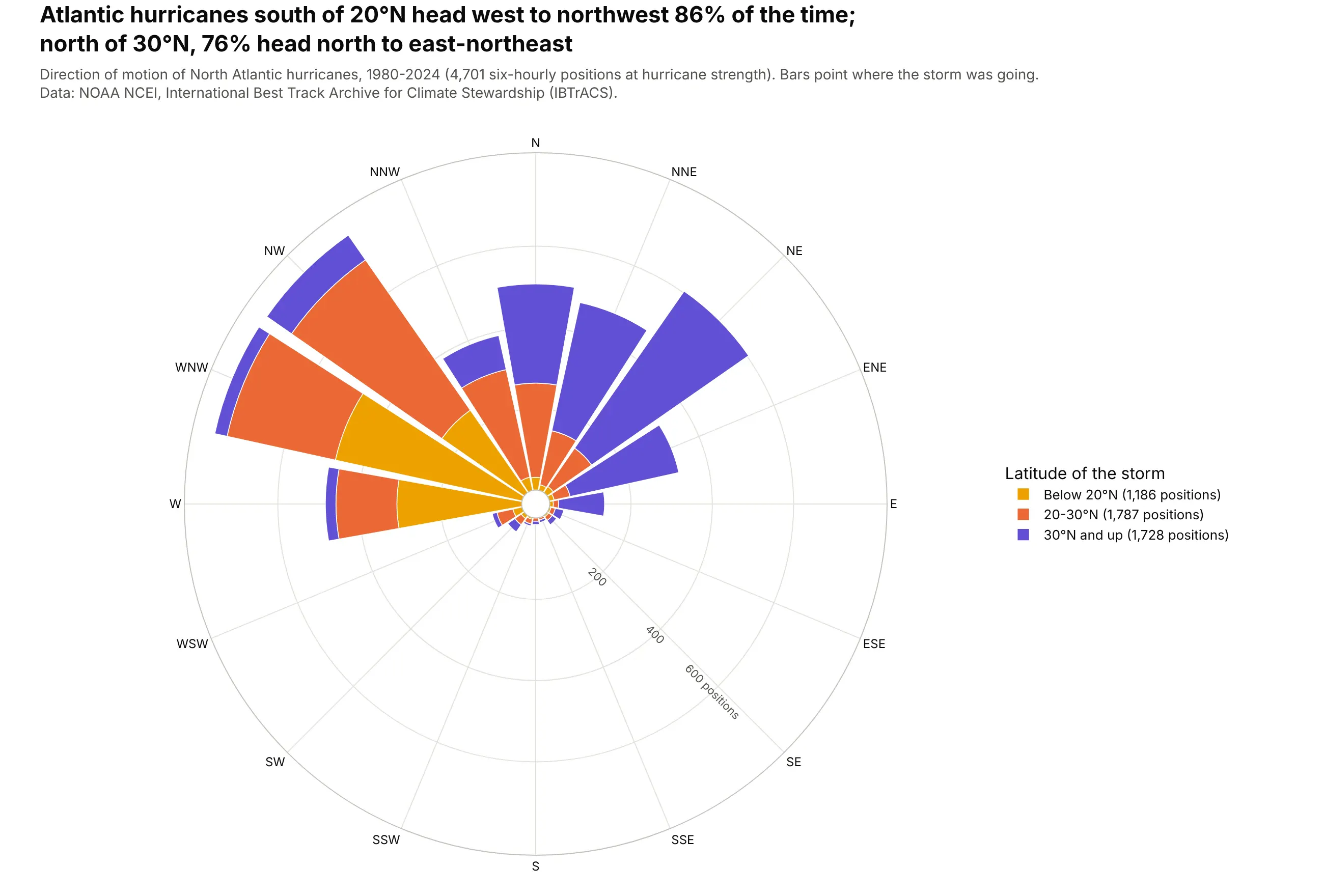
Below 20°N, hurricanes head west to northwest 86% of the time; north of 30°N, 76% head north to east-northeast. Stacking by latitude draws the typical recurving track in one rose. Unlike a wind rose, the bars point where storms go. Data: NOAA NCEI, IBTrACS (Knapp et al. 2010), 4,701 six-hourly positions.

Tip: stack by a category (here latitude band) with distinct colors instead of a sequence, because the bands aren't more or less of anything.

9. How gridded are New York's streets

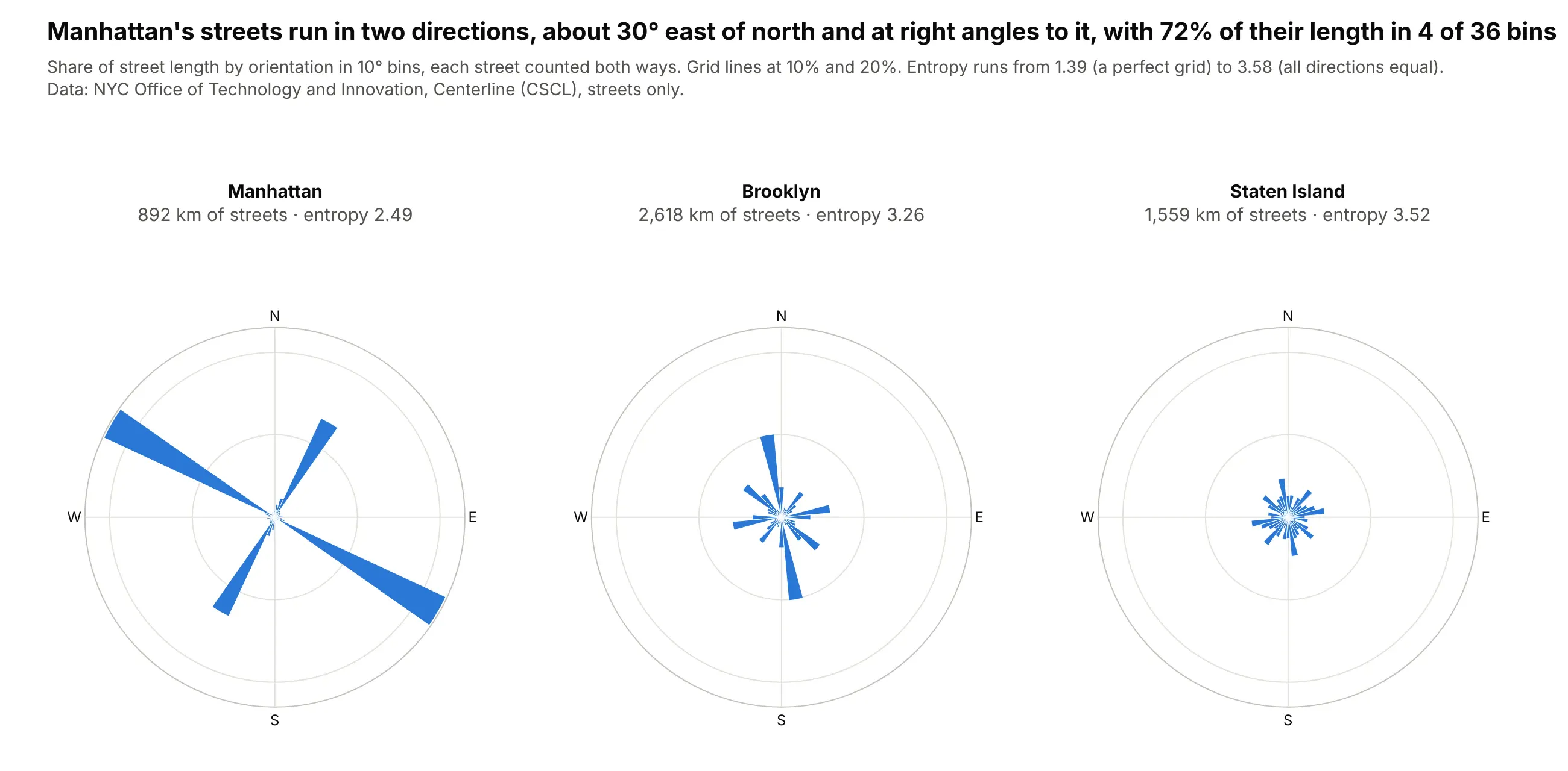
Manhattan's grid runs about 30° east of north, and 72% of its street length falls in 4 of 36 bins; Staten Island's streets point every way, with an orientation entropy of 3.52 against Manhattan's 2.49. Streets have no direction, so each one counts at its bearing and the opposite one. Data: NYC Office of Technology and Innovation, Centerline (CSCL); method from Boeing (2019).

Tip: polar.bargap=0 with numeric theta and width=10 draws a true polar histogram with touching bins.

10. Home runs are pulled

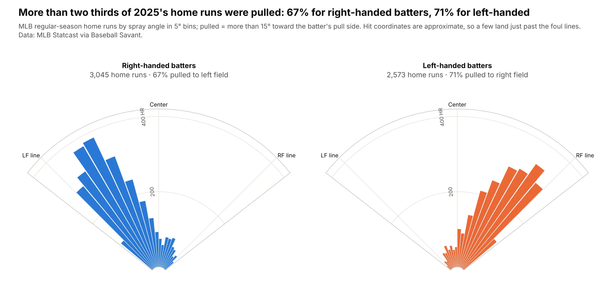
67% of right-handed batters' 3,045 home runs in 2025 went to left field, and 71% of left-handed batters' 2,573 to right field. A quarter-circle sector draws the field itself. Data: MLB Statcast via Baseball Savant, 2025 regular season.

Tip: polar.sector crops the polar axes to the field (here [38, 142], a little wider than fair territory for hits whose approximate coordinates land past the lines), and theta = 90 - spray_angle keeps left field on the left.