Chris Parmer

October 24, 2026

Beeswarm Plots - A Complete Guide

TL;DR

A beeswarm plot puts every item at its value on one axis and moves the dots sideways just enough that none overlap, so the swarm takes the shape of the distribution and every dot is still one named thing.
Beeswarm plots are also known as swarm plots and bee swarm plots, and are similar to strip plots, violin plots and histograms.
Use one for tens to a few thousand named items, such as companies, countries, drugs, hospitals or senators. For tens of thousands of points, use a histogram or a violin plot.
You can make a beeswarm plot with Plotly from one go.Scatter trace and a short function that computes the offsets. px.strip is the one-line version, but its jitter lets dots overlap.
Any coding agent can make one with Plotly in a minute if you ask for no-overlap offsets instead of jitter.

What is a beeswarm plot?

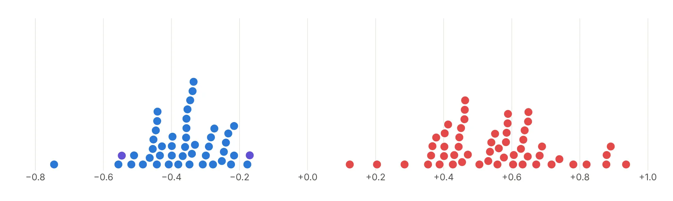
Beeswarm plots look like this:

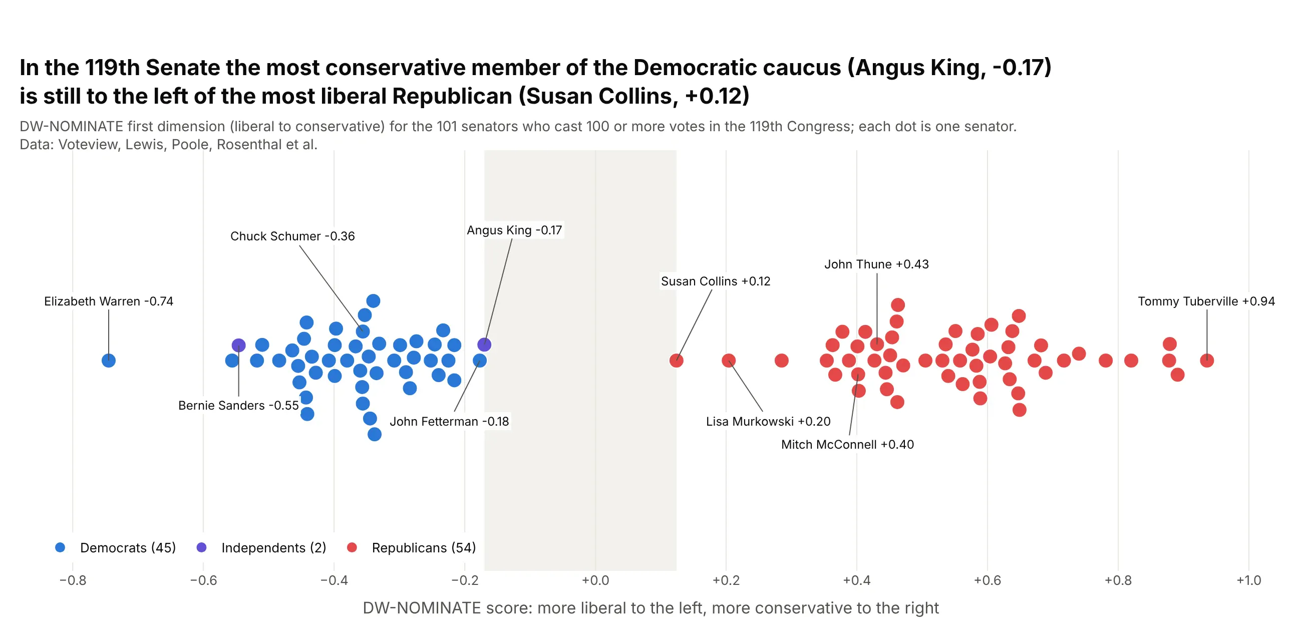
Beeswarm of 101 senators of the 119th Congress by DW-NOMINATE score, Democrats in blue, independents in purple and Republicans in red, with a shaded empty gap between Angus King at -0.17 and Susan Collins at +0.12, and ten senators labeled

Data: Voteview (Lewis, Poole, Rosenthal et al.), DW-NOMINATE scores for the 119th Congress.

How do you read a beeswarm plot? In the example above, notice these things:

Each dot is one senator of the 119th Congress, colored by party, with Democrats in blue, independents in purple and Republicans in red.
The horizontal position is the only thing that carries data. It is the senator's DW-NOMINATE score from their votes, so Elizabeth Warren sits far to the left as the most liberal senator and Tommy Tuberville far to the right as the most conservative.
The up-and-down position means nothing, because the dots are only pushed apart so they don't cover each other. The swarm gets taller where many senators have similar scores, which is why the Republicans form two tall clusters, one around Mitch McConnell and John Thune and a second a little further to the right.
The shaded band in the middle is where the two parties would overlap, and it is empty. Angus King, an independent who caucuses with the Democrats, is the dot closest to it on the left, and Susan Collins, at +0.12, is the closest on the right.
A dot sitting far from its group, like Warren's, is a single senator, so give it less weight than the clusters when you describe a whole party. The labels help you find the senators you know, and in an interactive Plotly version you can hover over any other dot to see who it is.

It's often used for charts like these:

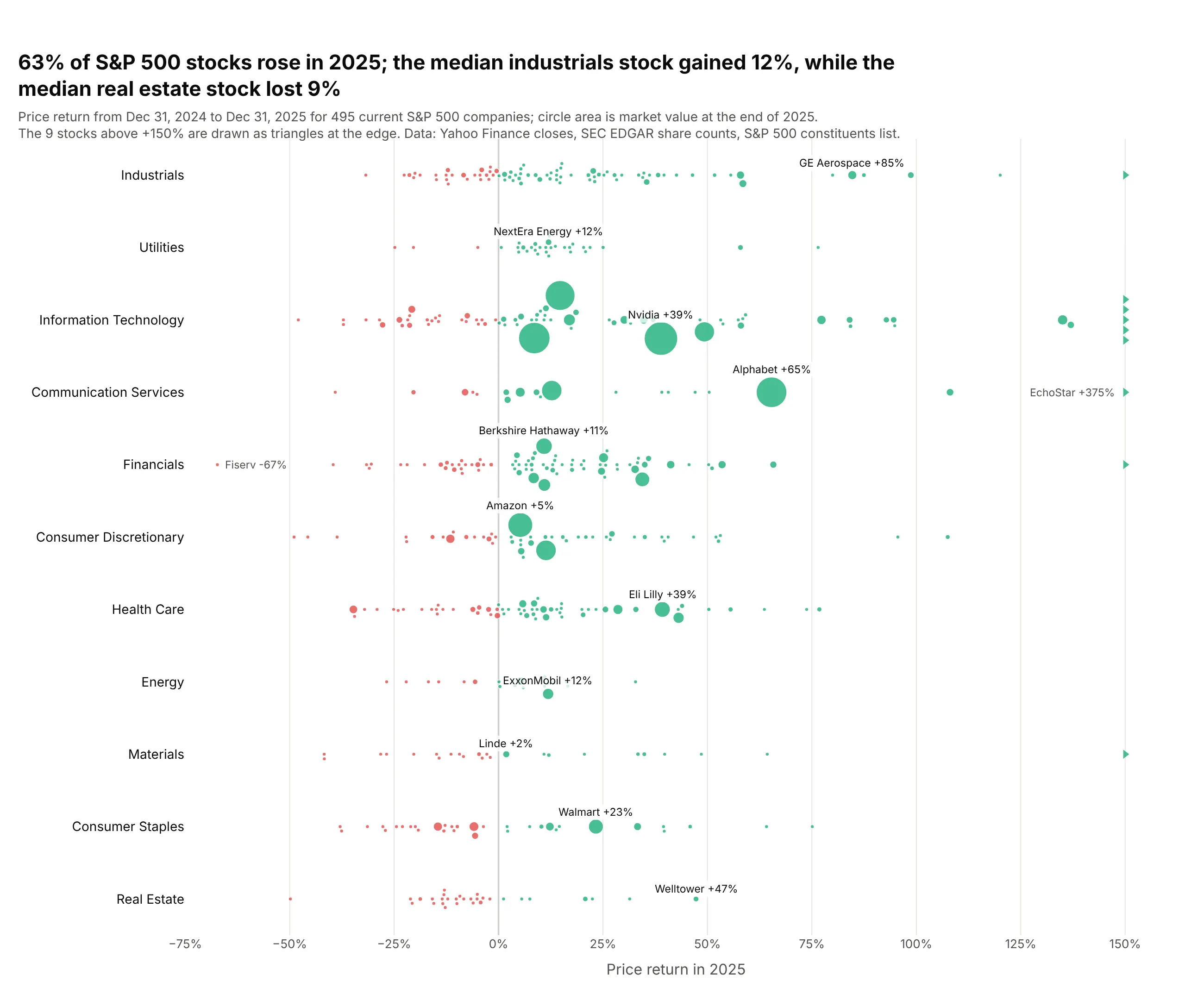
Beeswarm of 495 S&P 500 companies' 2025 price returns in one row per sector, circle area by market value, green for gains and red for losses. Industrials has the highest median and real estate the lowest; Nvidia (+39%) and Alphabet (+65%) are the biggest circles, and nine stocks above +150% sit as triangles at the right edge

Stock returns by sector. 312 of the 495 current S&P 500 companies (63%) rose in 2025, and sizing each dot by market value shows where the index's weight sat: Nvidia +39%, Alphabet +65%. Data: Yahoo Finance closes, SEC EDGAR share counts, S&P 500 constituents list.

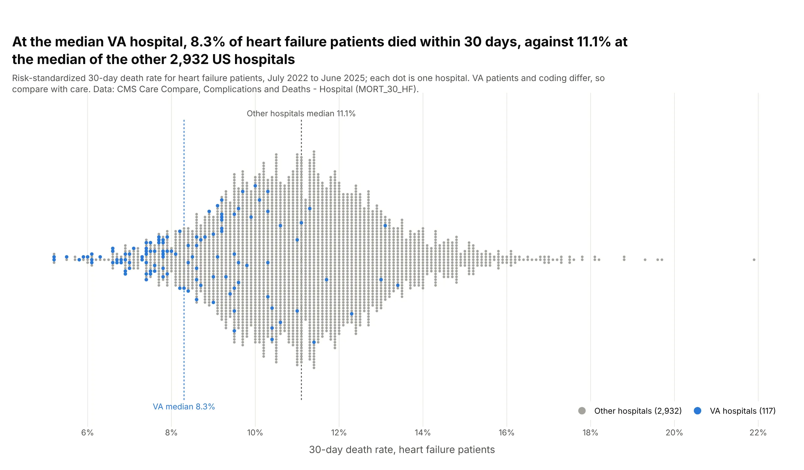
Beeswarm of 3,049 US hospitals' 30-day death rates for heart failure patients, small gray dots forming a diamond shape centered near 11%, with 117 VA hospitals in blue concentrated on the low side; dotted lines mark medians of 8.3% for VA and 11.1% for other hospitals

Thousands of hospitals on one measure. At the median VA hospital, 8.3% of heart failure patients died within 30 days, against 11.1% at the median of the other 2,932 US hospitals. Data: CMS Care Compare, MORT_30_HF, July 2022 to June 2025.

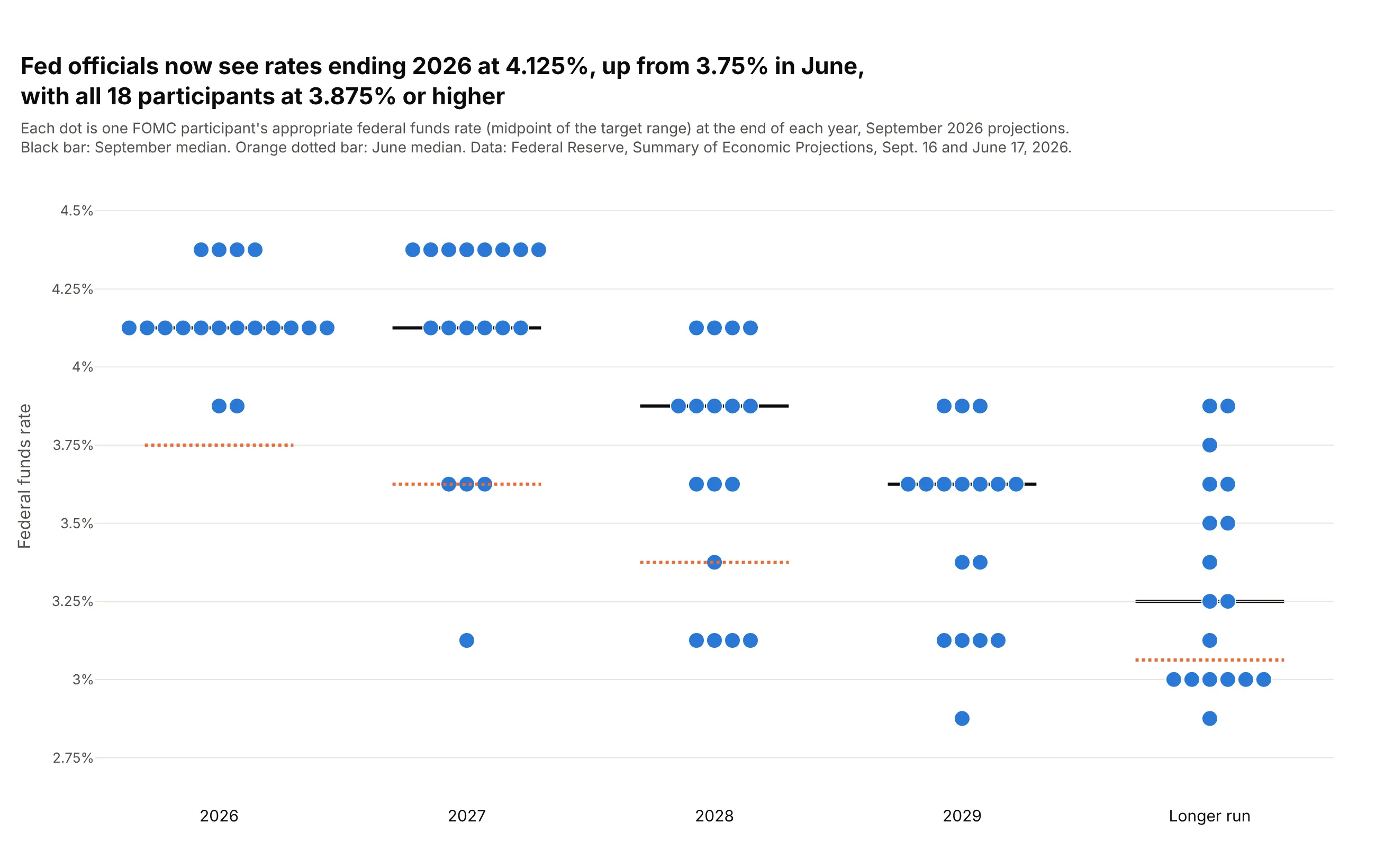
Beeswarm of FOMC participants' federal funds rate projections from September 2026, one column per year from 2026 to the longer run. The 2026 column has 12 dots at 4.125%, 4 at 4.375% and 2 at 3.875%; black bars mark September medians and orange dotted bars June medians, which were lower in every year June projected

Projections that land on a grid. The Fed's own "dot plot" is a beeswarm of officials' rate projections: the September 2026 median for the end of 2026 is 4.125%, up from 3.75% in June. Data: Federal Reserve, Summary of Economic Projections.

A short history

Leland Wilkinson described stacked dot plots and an algorithm for drawing them in The American Statistician in 1999. Aron Eklund's R package beeswarm, on CRAN since at least October 2010, gave the chart its name and kept each dot at its exact value instead of a bin center, and Python's seaborn library added the same idea as swarmplot (Waskom 2021). The chart works because it shows data as position on a common scale, the most accurate encoding in Cleveland and McGill's experiments (1984).

Alternatives to a beeswarm plot

Here's the same Senate drawn six ways. Some are better for the question, some worse, some just different:

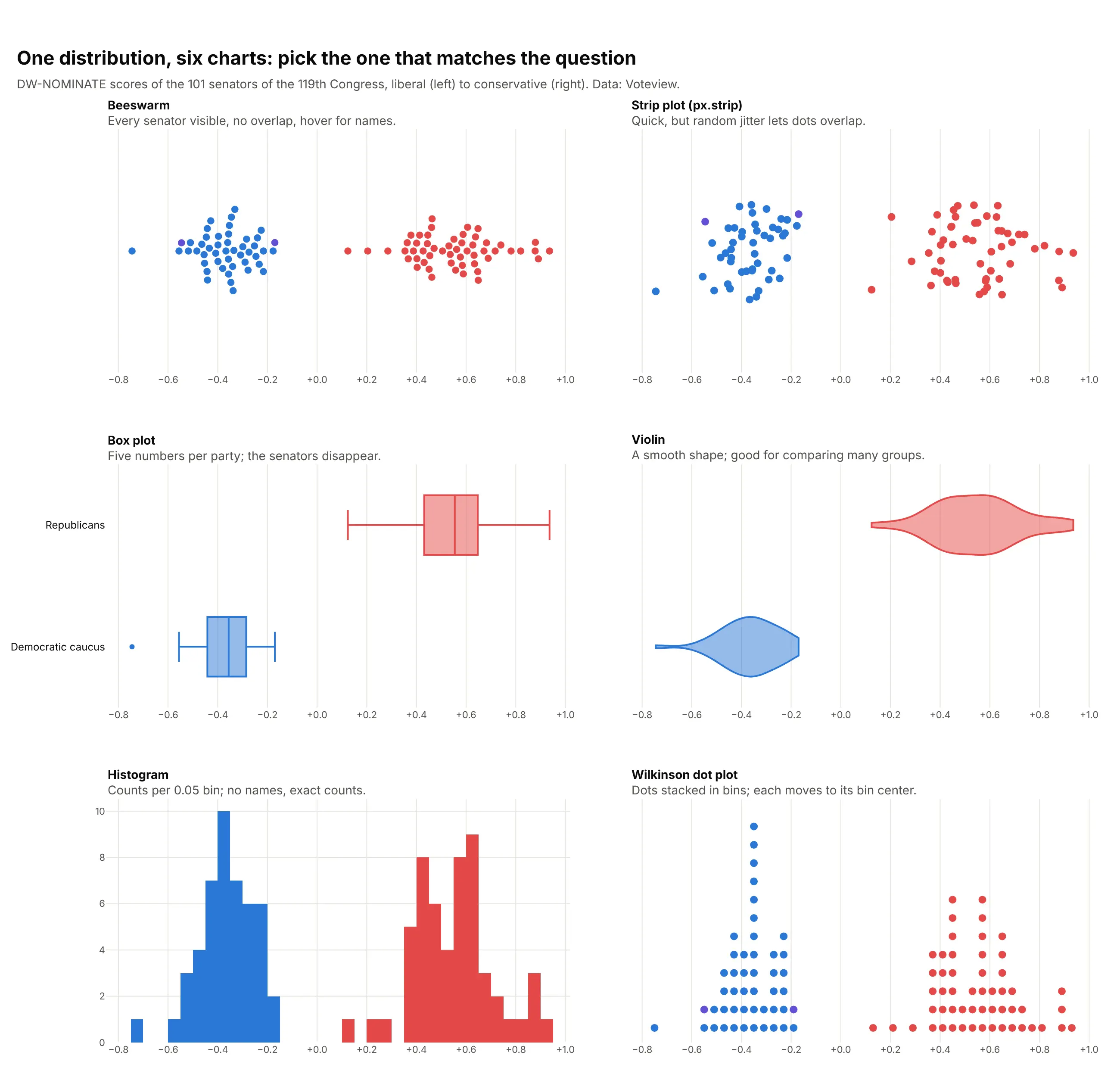
The 101 senators of the 119th Congress drawn six ways on the same DW-NOMINATE axis: a beeswarm, a jittered strip plot where dots overlap, box plots and violins for the two parties, a stacked histogram with 0.05 bins and a Wilkinson dot plot with dots stacked at bin centers

Strip plot (worse for publishing). px.strip spreads dots with jitter, so some overlap. It's fine for a first look.
Box plot (better for many groups). Five numbers per group compare well side by side, but the senators disappear, and with small groups the quartiles hide how few points there are.
Violin plot (better for big n). A smooth outline of the same shape. It needs no layout step and works for any number of points, but no dot can be hovered or labeled.
Histogram (better for exact counts). Bars read off an axis, so "how many senators score between 0.4 and 0.45" has an answer. Names are gone, and the shape depends on the bin width.
Wilkinson dot plot (works too). Dots stacked in bins keep the count visible and each dot hoverable, but every dot moves to its bin's center, so close values look equal.

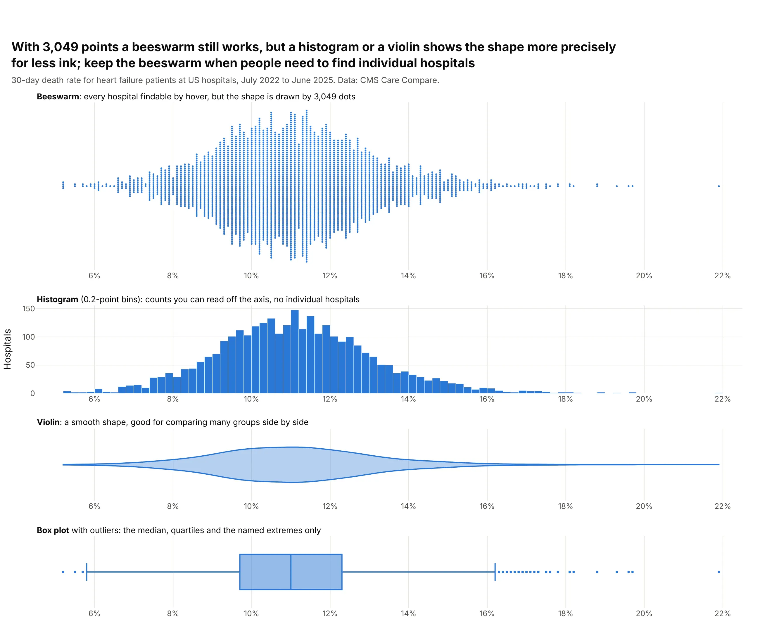
Here's where the histogram wins. With 3,049 hospitals the beeswarm still works, but the histogram shows the shape more precisely with less ink:

The same 3,049 hospital heart failure death rates drawn four ways: as a beeswarm of 3 px dots, as a histogram with 0.2-point bins, as a violin and as a box plot with outliers

How to make a beeswarm plot

With AI

ChatGPT, Claude Code, GitHub Copilot, Cursor and other AI tools are excellent at writing Plotly code. Name Plotly in the prompt, and ask for computed offsets, because "beeswarm" alone often gets you a jittered strip plot:

Make a plotly beeswarm plot from companies.csv (columns: ticker, company, sector, return_pct, market_cap_bn).

- No jitter. Convert values to pixels from a fixed plot width, take points in value order
  and put each at the free offset nearest the center line, so no two markers overlap.
- One row per sector, sorted by median return, with a short dark line at each median.
- Marker area proportional to market_cap_bn (largest 40 px, at least 4 px); use each marker's own
  diameter in the collision test, and draw big markers first.
- Green for gains, red for losses, a zero line, the largest company in each sector labeled.
- Fixed width, height and margins, and a title that states the takeaway.
- Check: assert that no two markers overlap and print the tallest swarm in pixels.

With Plotly Studio

Plotly Studio is a desktop app where you point an AI at a dataset and it builds charts and a Dash app around your questions. Ask for a beeswarm the same way:

Show a beeswarm plot of hospitals' 30-day heart failure death rates, one dot per hospital with no overlapping dots (not jitter), VA hospitals highlighted in blue and the rest gray, a dotted line at each group's median, and the hospital name on hover.

Make a beeswarm plot in Python or JavaScript

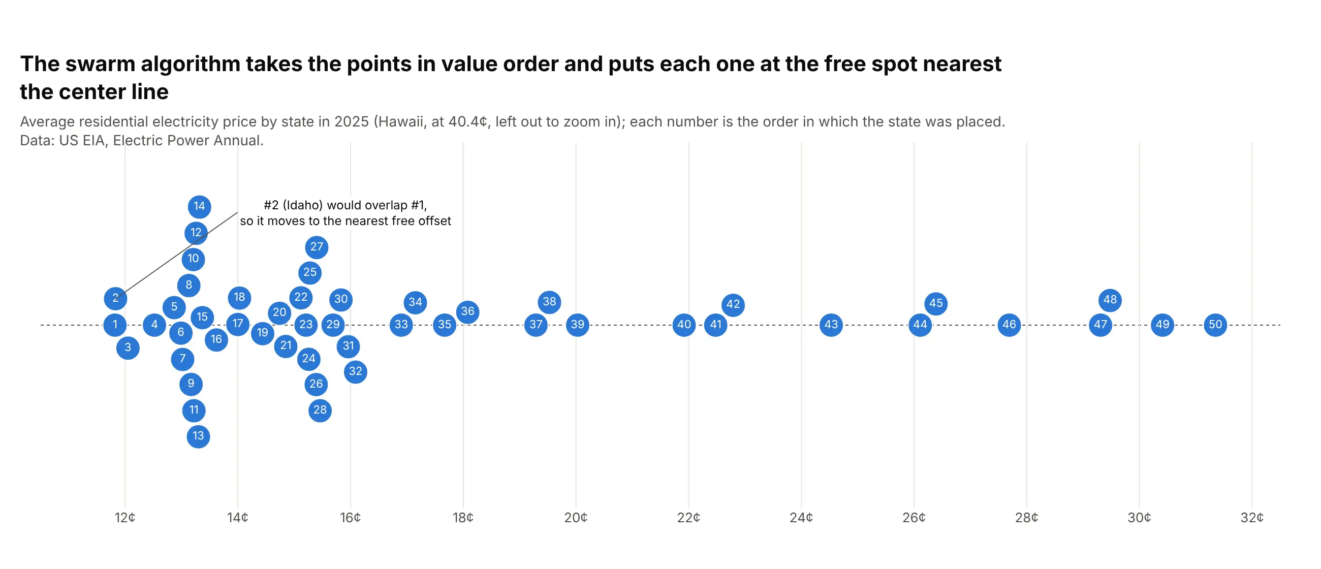
This is the code AI tools write under the hood. A beeswarm is a scatter trace, and the work is computing offsets: convert values to pixels, take the points in value order and put each one at the free offset nearest the center line. The candidates for a point are 0 and, for each placed neighbor close enough to collide, the two offsets where the new dot just touches it:

49 US states and DC by residential electricity price (Hawaii left out to zoom in), each dot numbered in the order the algorithm placed it: #1 sits on the center line, #2 (Idaho) would overlap #1 so it moves up, and the stacks grow where many states have similar prices

In Python, this helper does it and returns a go.Figure with one row per group:

import numpy as np
import pandas as pd
import plotly.graph_objects as go

def swarm_offsets(x_px, size_px, gap=1.0):
    """In value order, put each marker at the free offset nearest 0 (all in pixels)."""
    x_px = np.asarray(x_px, float)
    r = np.broadcast_to(np.asarray(size_px, float) / 2, x_px.shape)
    order = np.argsort(x_px, kind="stable")
    xs, rs, ys = x_px[order], r[order], np.zeros(len(order))
    lo = 0
    for i in range(len(xs)):
        while xs[i] - xs[lo] > 2 * rs.max() + gap:  # only nearby points can collide
            lo += 1
        nx, ny, dist = xs[lo:i], ys[lo:i], rs[i] + rs[lo:i] + gap
        close = np.abs(xs[i] - nx) < dist
        nx, ny, dist = nx[close], ny[close], dist[close]
        if len(nx):
            dy = np.sqrt(dist**2 - (xs[i] - nx) ** 2)
            cand = np.concatenate([[0.0], ny + dy, ny - dy])
            cand = cand[np.argsort(np.abs(cand), kind="stable")]
            ok = ((xs[i] - nx) ** 2 + (cand[:, None] - ny) ** 2 >= dist**2 - 1e-6).all(axis=1)
            ys[i] = cand[ok.argmax()]
    out = np.empty_like(ys)
    out[order] = ys
    return out

def make_beeswarm(df, x, group=None, text=None, size=8, width=1100, height=600,
                  margin=dict(l=170, r=30, t=60, b=50)):
    d = df.dropna(subset=[x]).copy()
    lo, hi = d[x].min(), d[x].max()
    lo, hi = lo - 0.03 * (hi - lo), hi + 0.03 * (hi - lo)
    groups = list(d[group].unique()) if group else [None]
    row_px = (height - margin["t"] - margin["b"]) / len(groups)
    d["_y"] = 0.0
    for i, g in enumerate(groups):
        m = d[group] == g if group else np.full(len(d), True)
        px = (d.loc[m, x] - lo) / (hi - lo) * (width - margin["l"] - margin["r"])
        d.loc[m, "_y"] = i + swarm_offsets(px, size) / row_px  # pixels -> row units
    fig = go.Figure(go.Scatter(x=d[x], y=d["_y"], mode="markers", text=d[text] if text else None,
                               marker=dict(size=size, line=dict(color="white", width=0.5))))
    fig.update_layout(width=width, height=height, margin=margin, template="simple_white")
    fig.update_xaxes(range=[lo, hi], showgrid=True)
    fig.update_yaxes(range=[len(groups) - 0.5, -0.5], tickvals=list(range(len(groups))),
                     ticktext=groups if group else [""], showline=False, ticks="")
    return fig

df = pd.read_csv("life_expectancy.csv")  # country, region, life_expectancy
fig = make_beeswarm(df, x="life_expectancy", group="region", text="country", size=9)

The offsets are in pixels, so the helper fixes the figure's width, height and margins. Every example in this guide builds on these two functions, adding color, labels, sized markers or a log axis (compute the pixels from log10 of the value).

In JavaScript, plotly.js draws the same thing from a scatter trace once the offsets are computed:

<div id="chart"></div>
<script src="https://cdn.plot.ly/plotly-4.1.1.min.js"></script>
<script>
  // 2026 OPS of the 17 qualified MLB shortstops (MLB Stats API)
  const names = ["Ezequiel Tovar", "Masyn Winn", "Andrés Giménez", "Trea Turner", "Xander Bogaerts",
    "Colson Montgomery", "Brayan Rocchio", "Gunnar Henderson", "Willy Adames", "Geraldo Perdomo",
    "Zach Neto", "Mookie Betts", "Otto Lopez", "Bobby Witt Jr.", "Kevin McGonigle", "CJ Abrams", "Elly De La Cruz"];
  const ops = [0.617, 0.625, 0.65, 0.675, 0.676, 0.685, 0.704, 0.712, 0.713, 0.747, 0.766, 0.78,
    0.786, 0.8, 0.806, 0.833, 0.88];

  const W = 800, H = 300, M = {l: 40, r: 30, t: 20, b: 40}, size = 22, lo = 0.6, hi = 0.9;
  const px = ops.map(v => (v - lo) / (hi - lo) * (W - M.l - M.r));
  // in value order, put each dot at the free offset nearest 0 (pixels)
  const y = [];
  ops.map((v, i) => i).sort((a, b) => px[a] - px[b]).forEach(i => {
    const near = Object.keys(y).filter(j => Math.abs(px[j] - px[i]) < size);
    const cand = [0];
    near.forEach(j => { const dy = Math.sqrt(size ** 2 - (px[j] - px[i]) ** 2); cand.push(y[j] + dy, y[j] - dy); });
    cand.sort((a, b) => Math.abs(a) - Math.abs(b));
    y[i] = cand.find(c => near.every(j => (px[j] - px[i]) ** 2 + (y[j] - c) ** 2 >= size ** 2 - 1e-6));
  });

  Plotly.newPlot("chart", [{
    type: "scatter", mode: "markers", x: ops, y: y.map(o => o / (H - M.t - M.b)), text: names,
    marker: {size: size, color: "#2a78d6", line: {color: "white", width: 1}},
    hovertemplate: "%{text}: %{x:.3f}<extra></extra>"
  }], {
    width: W, height: H, margin: M, showlegend: false,
    xaxis: {range: [lo, hi], title: {text: "OPS"}}, yaxis: {range: [-0.5, 0.5], visible: false}
  });
</script>

Share it

Every Plotly chart has a Share chart button (the cloud icon in its toolbar) that uploads it to Plotly Cloud and gives you a link. Only you can see it until you change its visibility.

For a live app, put the chart in a Dash app and publish it with the Plotly Cloud CLI. Coding agents can run these commands for you:

pip install "dash[cloud]"
plotly user login
plotly app publish

If your data has to stay in your own cloud or data center, publish to Dash Enterprise instead.

Dos and don'ts

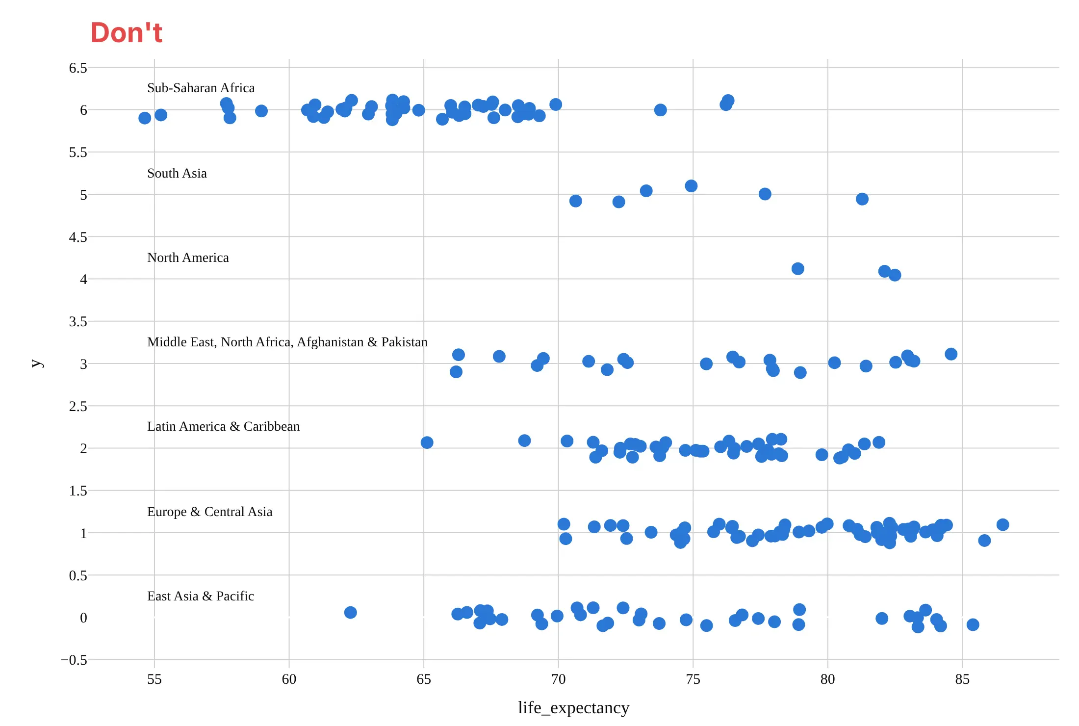
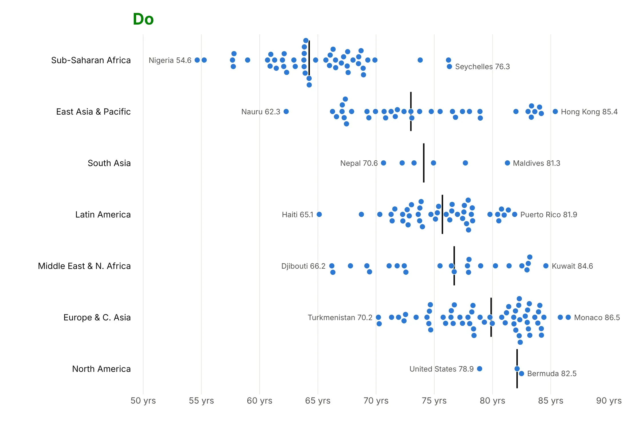
Most of the work in a published beeswarm is placement, order and what to label. Here are 217 countries' life expectancy both ways, in the same color.

Don't use jitter that lets dots overlap, leave the groups in alphabetical order, show tick marks and gridlines on the offset axis (its numbers mean nothing), or use a default serif font and raw column names as axis titles:

Life expectancy of 217 countries as a jittered strip plot: dots overlap, regions are in alphabetical order with names floating above each row, the vertical axis shows meaningless numbers from -0.5 to 6.5 with gridlines, and the text is in a serif font with the axis title life_expectancy

Do compute the offsets so no dot overlaps, sort the groups by their median, mark each median, label the lowest and highest country in each group and hide the offset axis:

The same 217 countries as a beeswarm with no overlap, one row per region sorted from Sub-Saharan Africa (median 64.3) to North America, a dark median tick on each row, and the lowest and highest country of each region labeled, from Nigeria at 54.6 years to Monaco at 86.5

Use color and labels for one job

The same 101 senators, styled four ways. Each answers a different question.

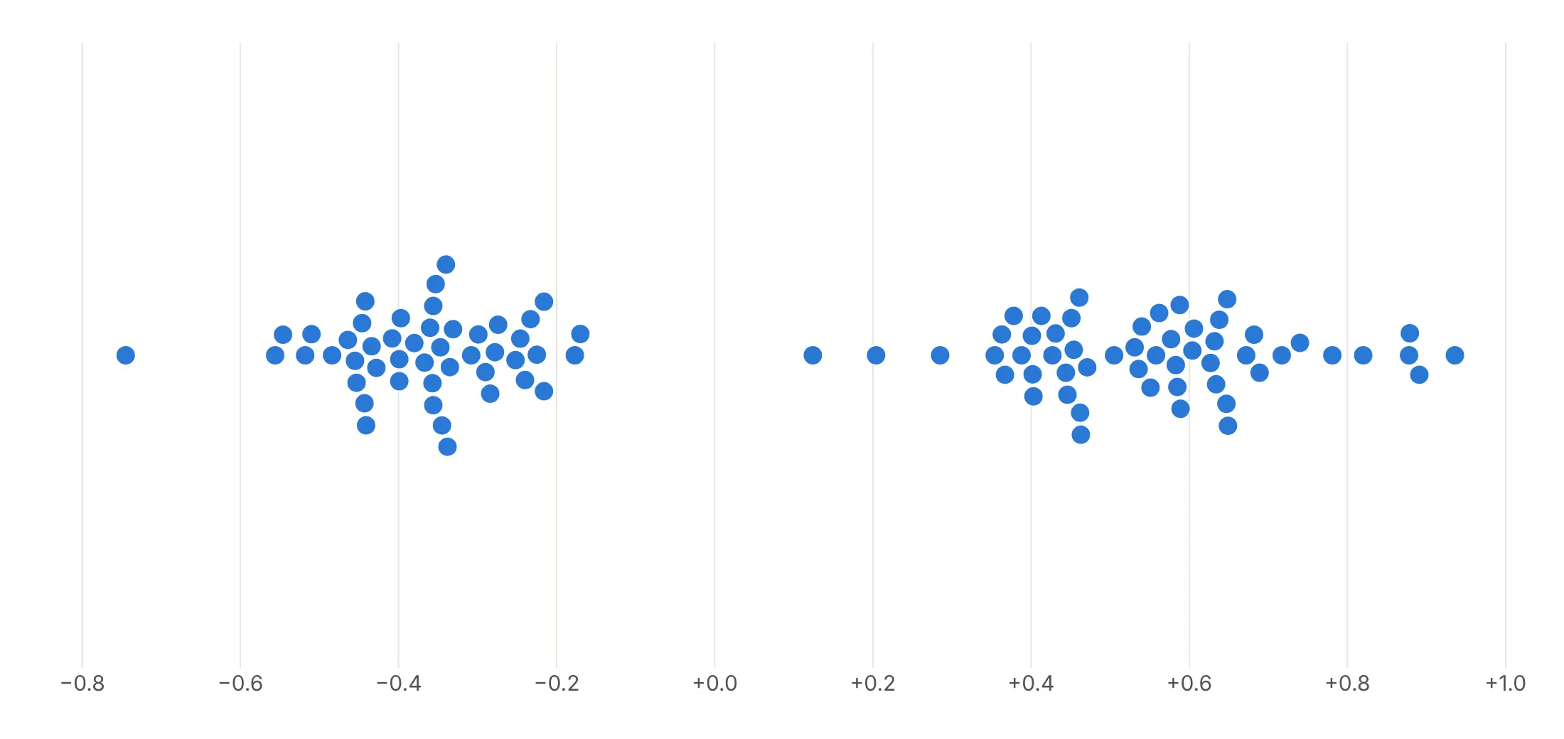
One color. Shows the shape of the chamber and nothing else, a good start before you know the story.

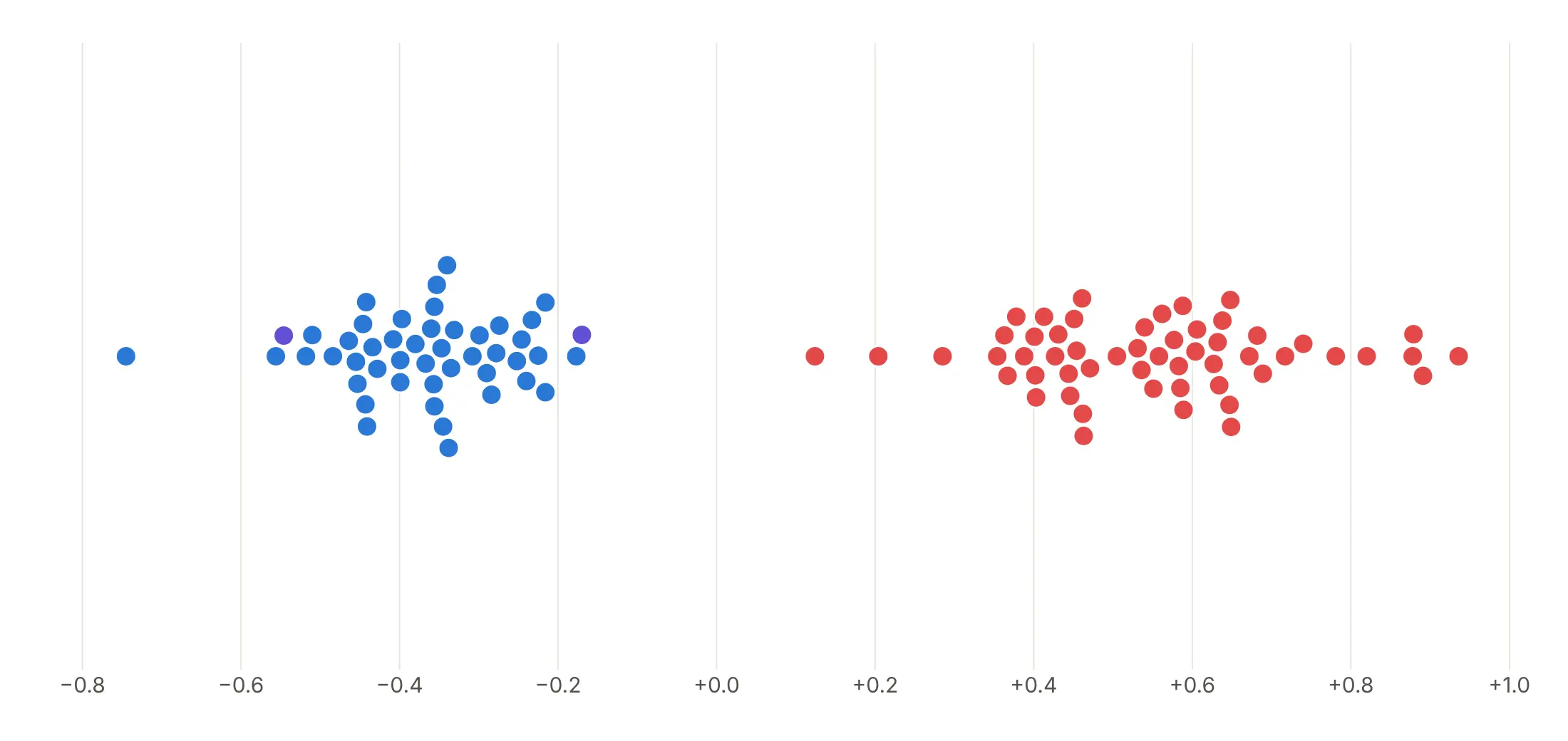
The 101 senators as a beeswarm in one blue, with two clusters separated by an empty gap

Color by group. Party colors show that the gap between the clusters is the gap between the parties.

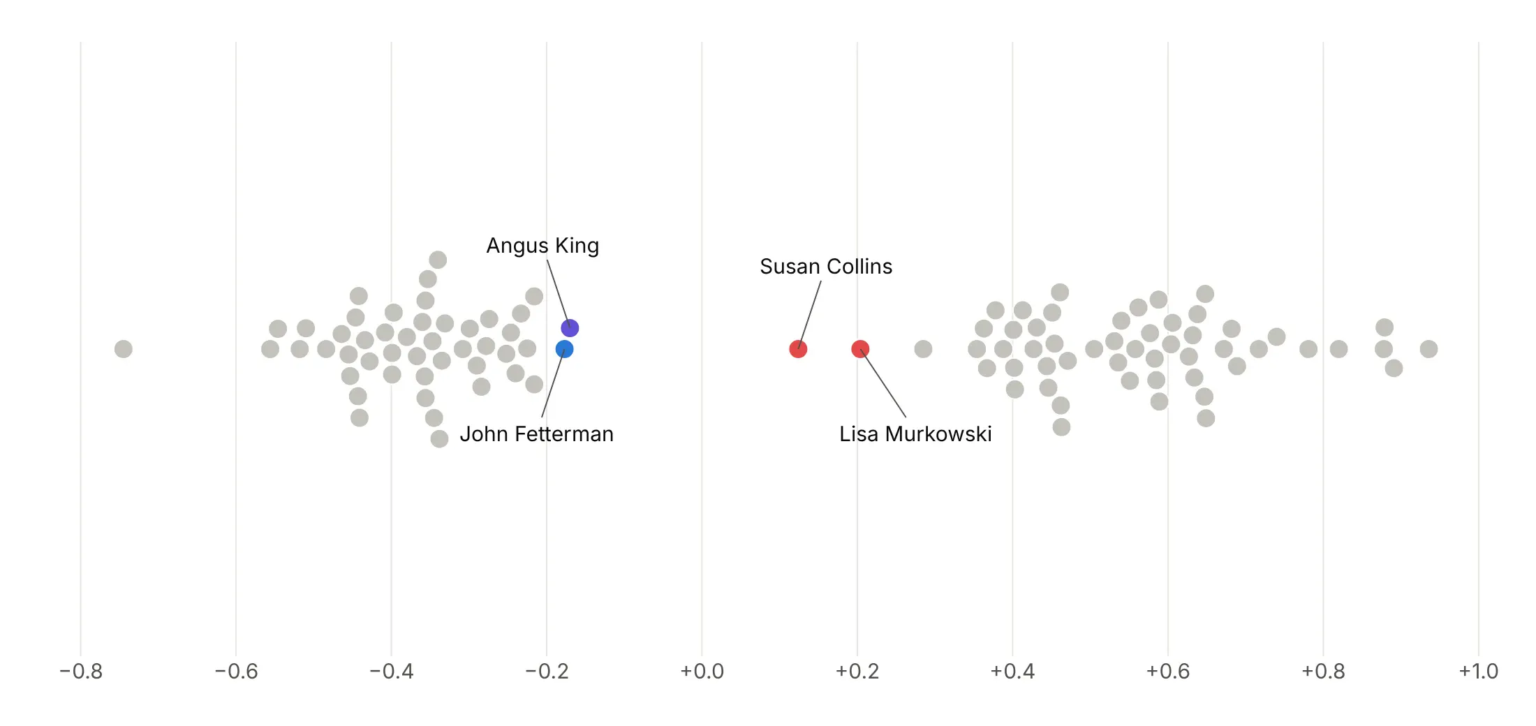
The same beeswarm with Democrats in blue, the two independents in purple and Republicans in red

Highlight and label a few. Gray the rest so the four senators closest to the center stand out: Angus King, John Fetterman, Susan Collins and Lisa Murkowski.

The same beeswarm in gray with Angus King, John Fetterman, Susan Collins and Lisa Murkowski in their party colors and labeled

One-sided swarm. Stacking dots upward from a baseline turns the beeswarm into a dot histogram in which every dot can still be hovered.

The same senators stacked upward from a baseline, Democrats in blue and Republicans in red, like a histogram made of dots

Size the markers for the number of points

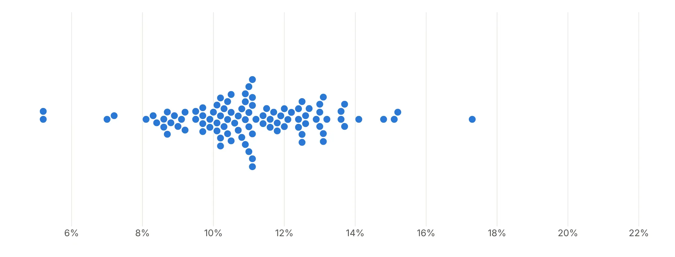
A swarm's height grows with how many points share a value, not with the plot. With 100 hospitals, 12 px markers with a white outline fit easily:

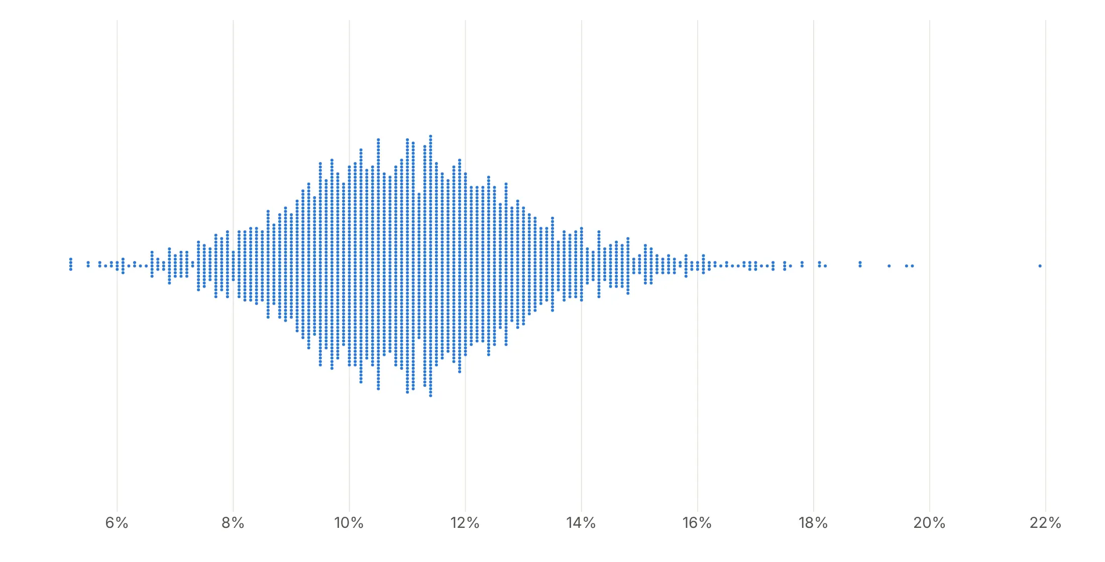
A random sample of 100 hospitals' heart failure death rates as a beeswarm of 12 px dots

With all 3,049 hospitals, the same death rates need 3 px markers with no outline, and the published rates' 0.1-point steps show as columns:

All 3,049 hospitals' heart failure death rates as a beeswarm of 3 px dots forming a diamond shape centered near 11%

Checklist

Compute the offsets with no overlap and a fixed order, so the chart looks the same every time.
Fix the figure's width, height and margins, because the offsets are in pixels.
Size markers for n: about 10-15 px up to 200 points, 5-8 px up to 1,000 and 3-4 px with no outline above that.
Sort groups by their median and mark it with a short line.
Label the dots the story needs, and put every item's name in the hover text.
Write a title that states the takeaway.

Don't

Use jitter that lets dots overlap for a published chart.
Give the offset axis tick labels or gridlines.
Color by the same thing the rows already show.
Stretch a beeswarm to fit a container without recomputing the offsets.

Options to customize

A beeswarm is a go.Scatter trace plus a layout, so these are the options that matter most. The full list is in the Plotly scatter plot documentation, and px.strip is in the strip chart documentation.

mode="markers": draws the dots; values on one axis, computed offsets on the other.
layout.width, height, margin: fix the pixel size the offsets were computed for.
marker.size: diameter in pixels, one value or one per point for sized swarms.
marker.line: a white outline of 0.5-1 px for small n, none above about 1,000 points.
marker.color: a category, a highlight or a direction; a list gives one color per dot.
marker.opacity: 0.8 or so when big sized markers sit near small ones.
marker.symbol: a different shape, for example triangles for values clipped at the axis edge.
mode="markers+text", textfont: short labels inside big markers, such as state codes.
text, customdata, hovertemplate: the item's name and details on hover.
yaxis.tickvals, ticktext, range: group labels at integer rows and a fixed range for grouped swarms.
yaxis.visible=False: hides the meaningless offset axis in single-row swarms.
xaxis.type="log": a log value axis; compute the pixels from log10 of the value.
layout.annotations (ax, ay, standoff): labels with leader lines; on a log axis pass log10(x).
add_shape, add_vline, add_vrect: median ticks, reference lines and shaded gaps.
px.strip: a strip plot with jitter, for a quick first look.
go.Scattergl: WebGL markers, for swarms of several thousand points.

More beeswarm plot examples

Nine more beeswarm plots built from real public data, each with its source, the technique that makes it work and a prompt to rebuild it.

1. Electricity prices in every state

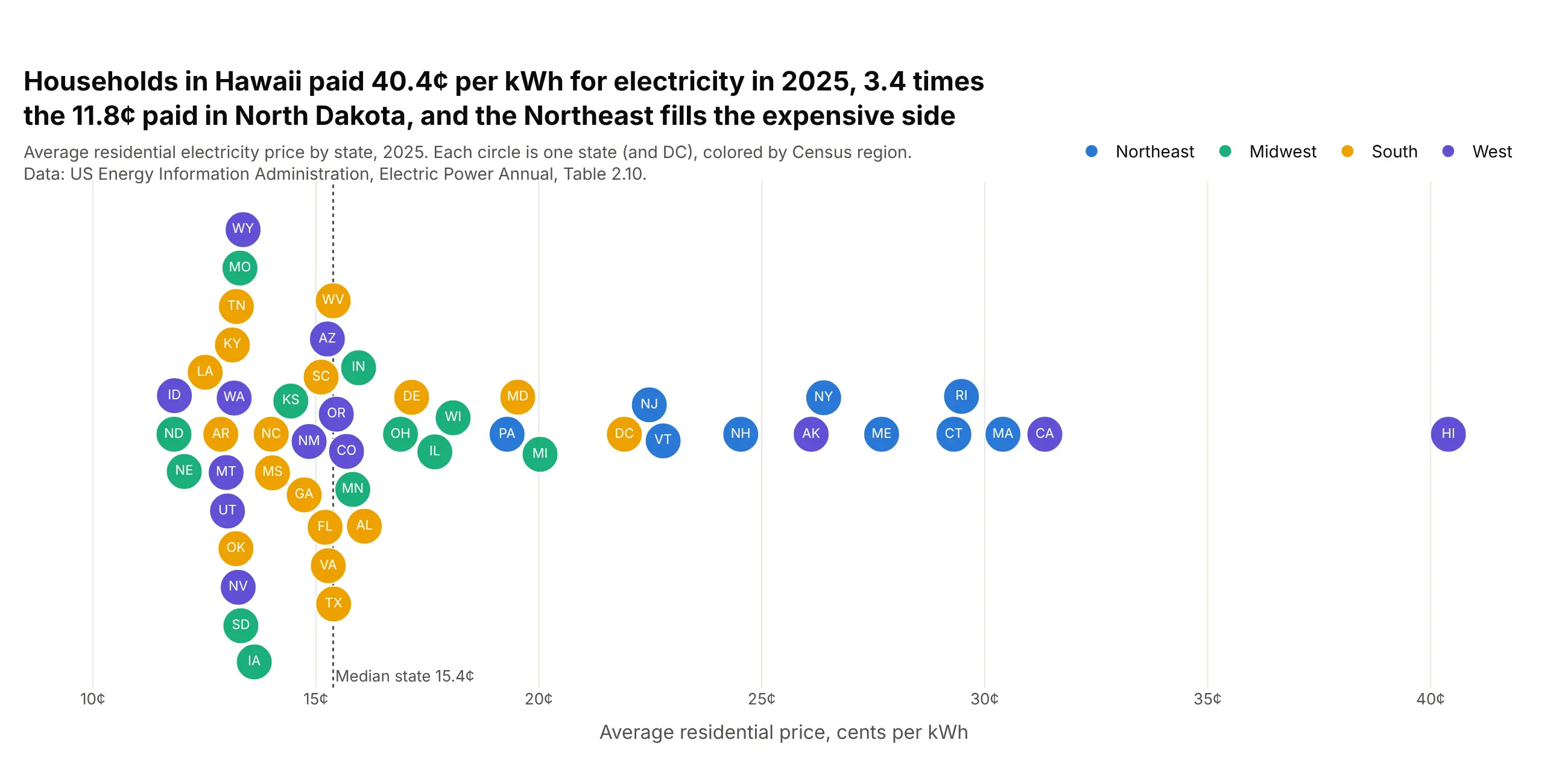
Beeswarm of 2025 average residential electricity prices in the 50 states and DC, with the two-letter state code inside each circle, colored by Census region. Most states cluster between 12 and 18 cents; Hawaii is alone at 40.4 cents and all nine Northeastern states sit between 19 and 31 cents

Households in Hawaii paid 40.4 cents per kWh in 2025, 3.4 times the 11.8 cents in North Dakota. Seven of the ten most expensive states are in the Northeast. Data: US EIA, Electric Power Annual, Table 2.10.

Tip: with about 50 items, make the markers big enough (30 px) to hold a two-letter label with mode="markers+text".

Get the data from the US EIA Electric Power Annual, Table 2.10 (average residential price by
state, 2025) and shape it into a table (columns: state, code, region, price_2025).

Build a plotly beeswarm: x = price (cents/kWh), 30 px circles with the state code in white,
colored by Census region, offsets computed so circles don't overlap. Dotted line at the median.

2. How much of each country's electricity is low-carbon

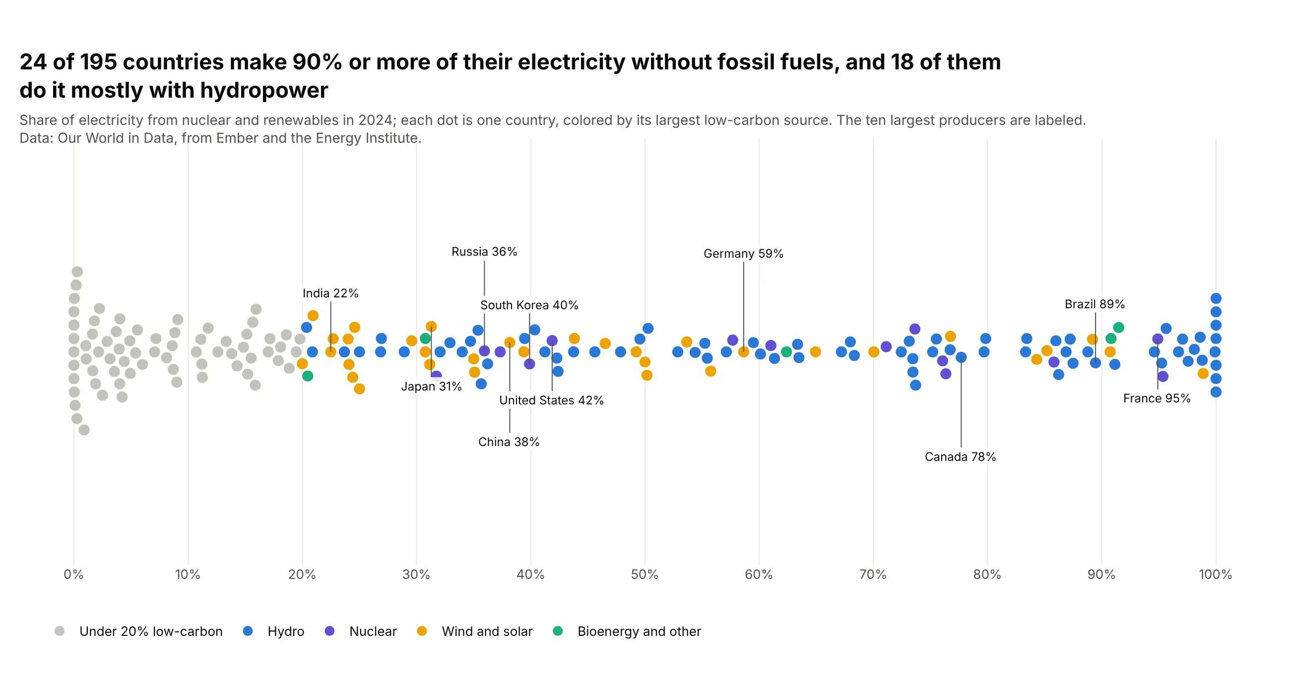
Beeswarm of 195 countries' share of electricity from nuclear and renewables in 2024, colored by largest low-carbon source, with countries under 20% in gray. A pile of gray fossil-heavy countries sits near 0%, a blue column of hydro countries near 100%, and the ten largest producers are labeled, from India at 22% to France at 95%

Twenty-four of 195 countries make 90% or more of their electricity without fossil fuels, and 18 of them do it mostly with hydropower. The ten largest producers, labeled, sit between India's 22% and France's 95%. Data: Our World in Data, from Ember and the Energy Institute.

Tip: gray out the countries where the "main source" is a small share, so color only appears where it means something.

Get the data from Our World in Data's energy dataset (github.com/owid/energy-data, from Ember and
the Energy Institute) and shape it into a table for 2024 (columns: country, generation_twh,
low_carbon_share, main_source), countries only.

Build a plotly beeswarm: x = low_carbon_share (%), color = main low-carbon source, gray under 20%.
Label the ten largest producers with leader lines, alternating above and below.

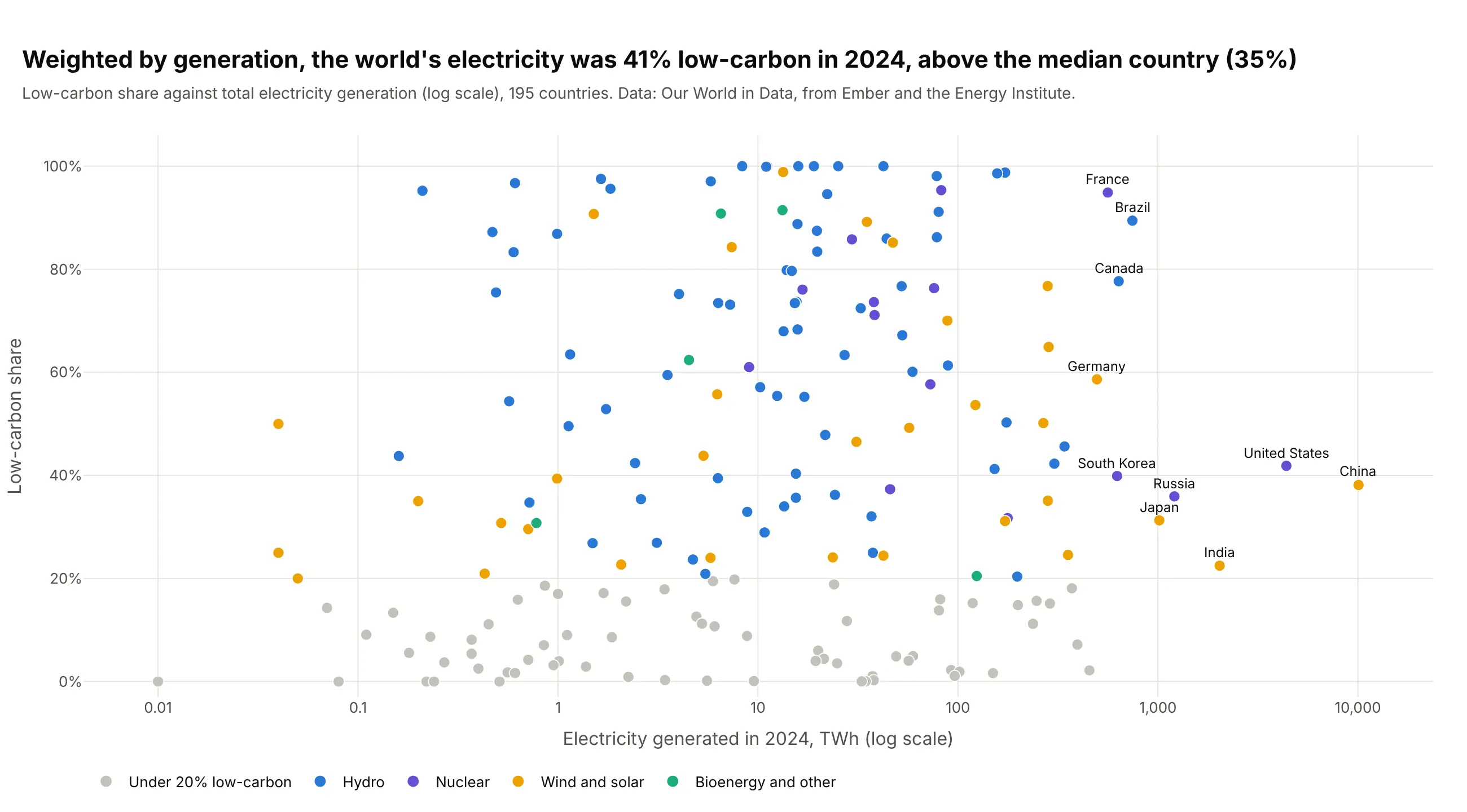
Another way to see it: a scatter plot against total generation adds the size the beeswarm leaves out, and shows that the generation-weighted share (41%) is above the median country (35%).

Scatter plot of low-carbon share against electricity generation on a log axis for 195 countries, with the ten largest producers labeled

3. Medicare drug prices, 2023 to 2024

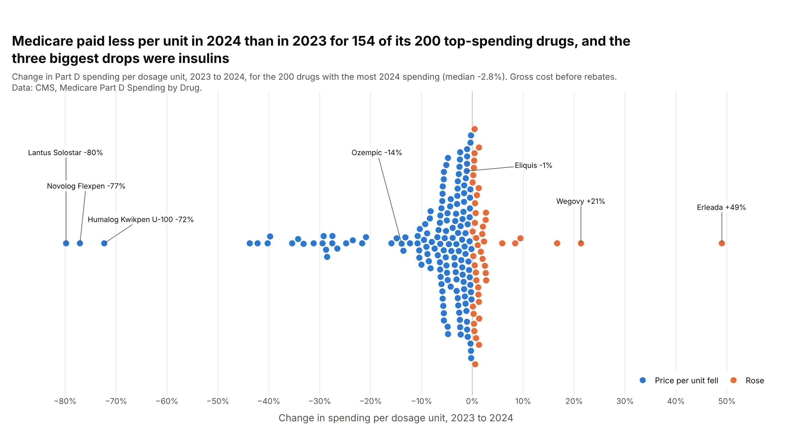
Beeswarm of the change in Medicare Part D spending per dosage unit from 2023 to 2024 for the 200 top-spending drugs, blue for falls and orange for rises. Most drugs sit between -10% and +3%; three insulins are far left at -72% to -80%, and Erleada is far right at +49%

Medicare paid less per unit in 2024 for 154 of its 200 top-spending drugs, with a median change of -2.8%. The three biggest drops were insulins (Lantus Solostar -80%, Novolog Flexpen -77%, Humalog Kwikpen -72%). Data: CMS, Medicare Part D Spending by Drug, gross of rebates.

Tip: two colors split at zero, and leader-line labels for the drugs at the ends and the two biggest by spending.

Get the data from CMS Medicare Part D Spending by Drug (data.cms.gov, "Overall" rows, data
years 2020-2024) and shape it into a table (columns: brand, generic, spend_2024_bn,
price_change_pct = Chg_Avg_Spnd_Per_Dsg_Unt_23_24 x 100) for the 200 drugs with the most 2024 spending.

Build a plotly beeswarm: x = price_change_pct, blue below 0, orange above, a zero line.
Label the three largest falls, the two largest rises, Eliquis and Ozempic.

4. Obesity drug trials by size

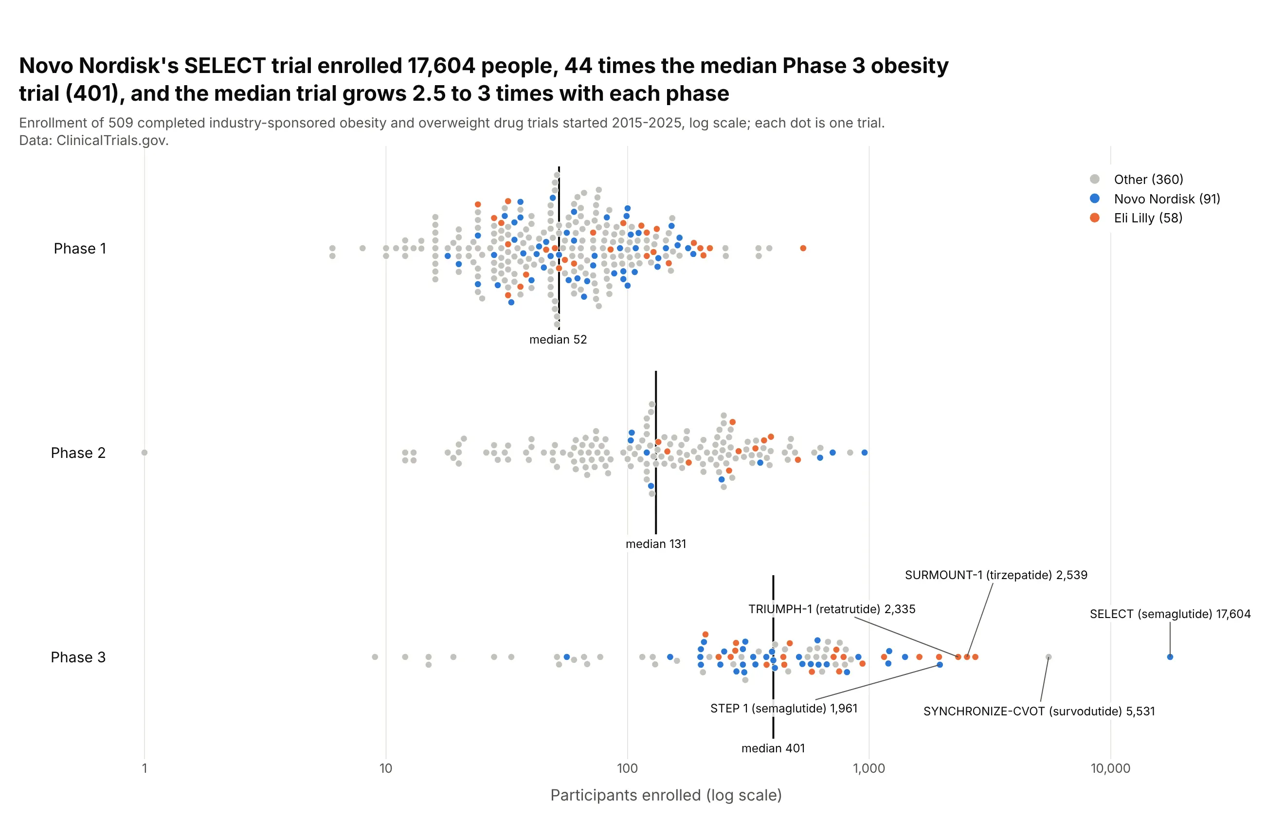
Beeswarm of 509 completed industry obesity drug trials by enrollment on a log axis, one row per phase, Novo Nordisk in blue, Eli Lilly in orange and other sponsors in gray. Medians are 52, 131 and 401 participants for Phases 1, 2 and 3; SELECT is far right at 17,604

Novo Nordisk's SELECT trial enrolled 17,604 people, 44 times the median Phase 3 obesity trial (401). The median trial grows 2.5 to 3 times with each phase. Data: ClinicalTrials.gov, completed industry trials started 2015-2025.

Tip: a log axis, with the pixel positions computed from log10(enrollment) so the swarm matches the axis.

Get the data from the ClinicalTrials.gov API v2 (interventional, industry lead sponsor,
completed, started 2015-2025, condition "obesity OR overweight", Phases 1-3) and shape it into
a table (columns: nct_id, acronym, title, sponsor, phase, enrollment).

Build a plotly beeswarm: one row per phase, x = enrollment on a log axis (offsets computed
from log10), Novo Nordisk blue, Eli Lilly orange, others gray, medians marked, the biggest
trials labeled with their acronyms.

5. Life expectancy by region

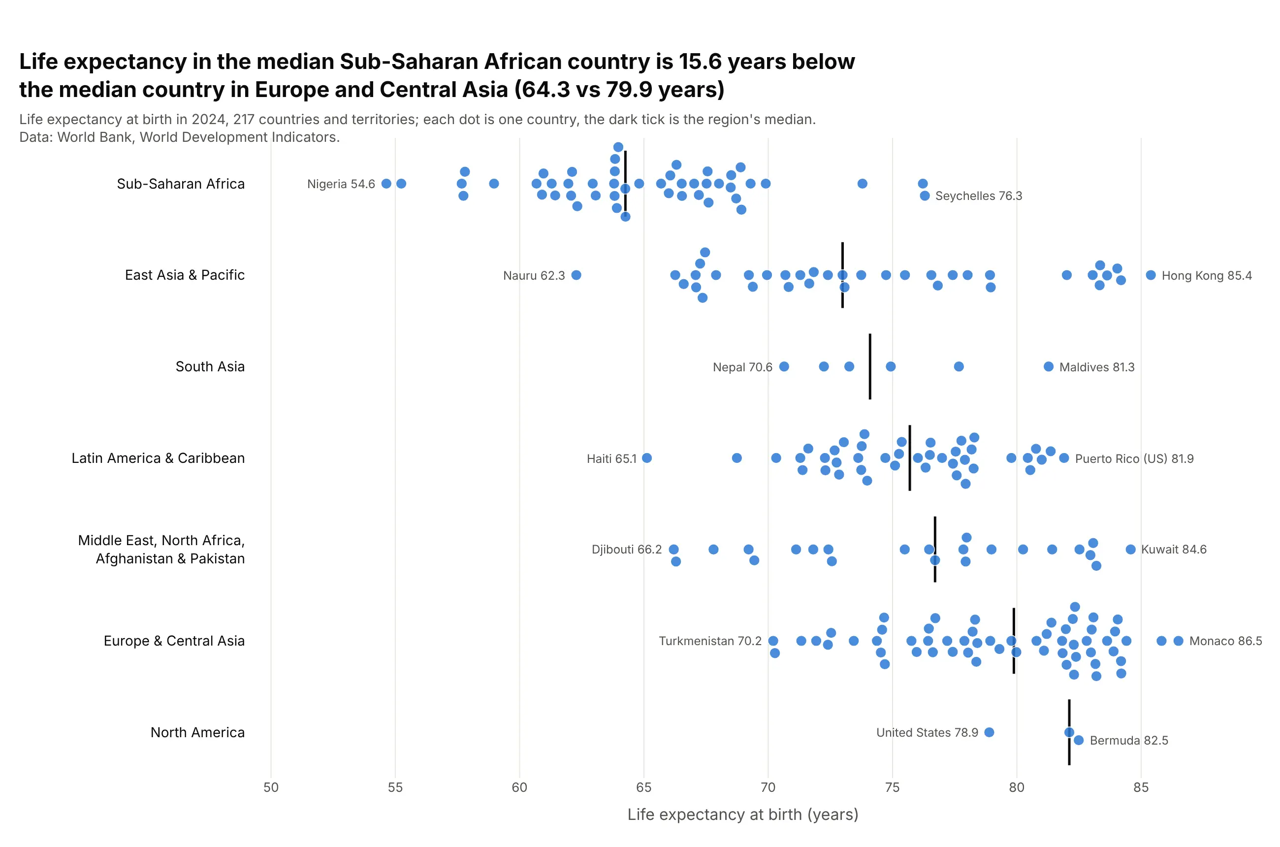
Beeswarm of 217 countries' life expectancy in 2024, one row per World Bank region sorted by median, with a dark median tick and the lowest and highest country of each region labeled, from Nigeria at 54.6 years to Monaco at 86.5

Life expectancy in the median Sub-Saharan African country is 15.6 years below the median country in Europe and Central Asia (64.3 vs 79.9). Every region has a long tail, such as Nauru (62.3) and Hong Kong (85.4) in East Asia. Data: World Bank, World Development Indicators, 2024.

Tip: label only each row's lowest and highest country, which names the range without crowding the swarm.

Get the data from the World Bank World Development Indicators (SP.DYN.LE00.IN for 2024, with
regions from the country metadata) and shape it into a table (columns: country, region, life_expectancy).

Build a plotly beeswarm: one row per region sorted by median, one blue color, 11 px markers,
a dark tick at each median, and the lowest and highest country of each region labeled.

6. Every magnitude 7+ earthquake since 2000

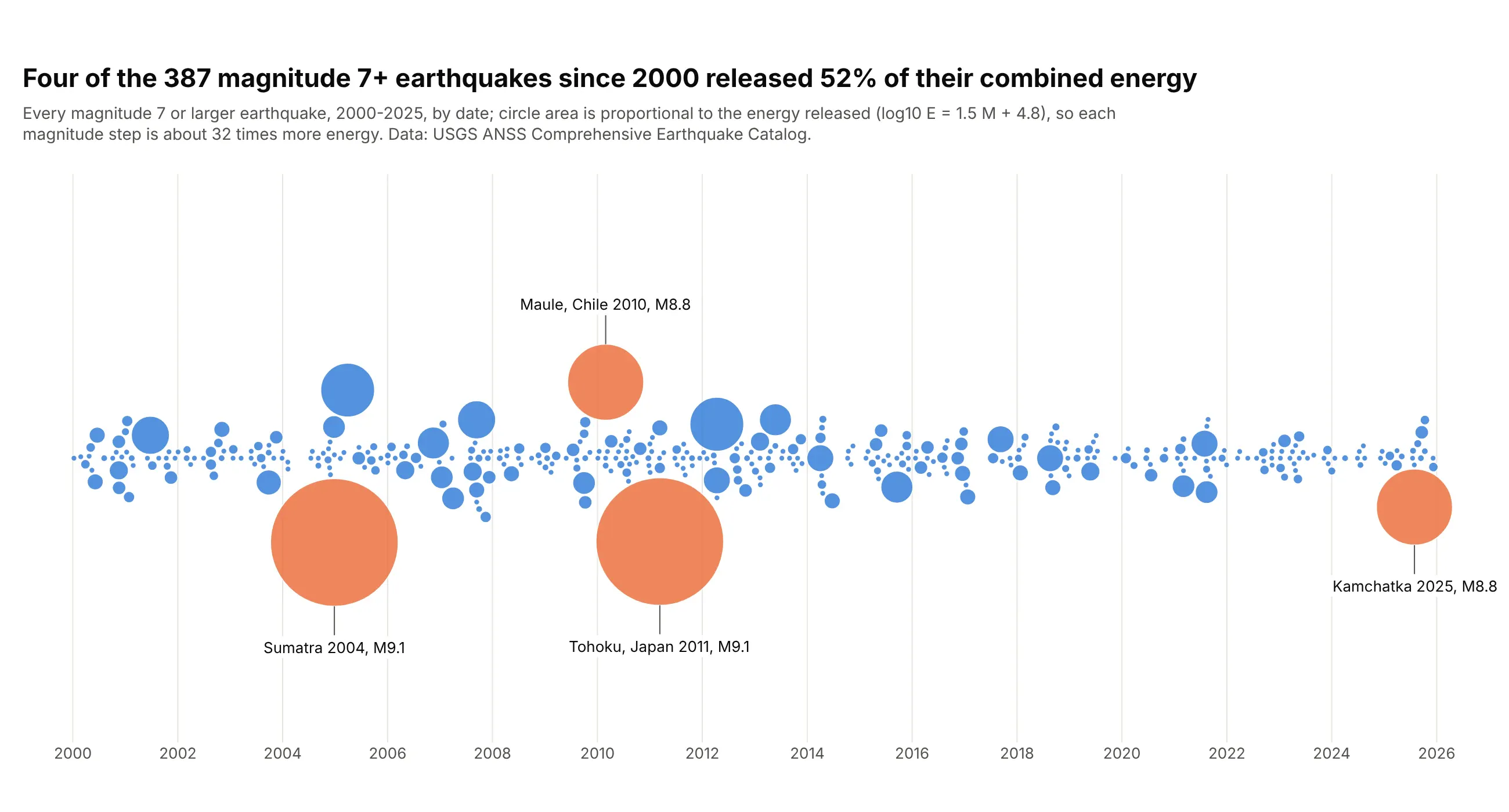
Beeswarm timeline of 387 magnitude 7+ earthquakes from 2000 to 2025, circle area proportional to energy released. Four large orange circles (Sumatra 2004, Maule 2010, Tohoku 2011, Kamchatka 2025) dwarf hundreds of small blue dots

Four of the 387 magnitude 7+ earthquakes since 2000 released 52% of their combined energy. On a time axis, the swarm keeps quakes that happened close together as separate dots. Data: USGS ANSS Comprehensive Earthquake Catalog.

Tip: size by the physical quantity (energy, from log10 E = 1.5 M + 4.8) and give the algorithm each marker's diameter.

Get the data from the USGS Comprehensive Earthquake Catalog (FDSN event service, magnitude 7+,
2000-2025) and shape it into a table (columns: time, mag, place, energy_pj = 10**(1.5*mag + 4.8) / 1e15).

Build a plotly beeswarm on a date axis: marker area = energy (largest 110 px, at least 5 px),
offsets computed with each marker's diameter, the four largest in orange with labels outside the swarm.

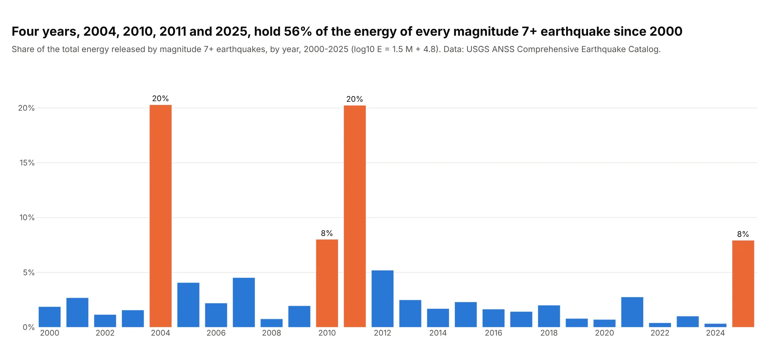
Another way to see it: a bar chart of energy by year puts a number on each year, 20% each for 2004 and 2011, but merges the quakes.

Bar chart of the share of magnitude 7+ earthquake energy released each year from 2000 to 2025, with 2004 and 2011 at 20% and 2010 and 2025 at 8% in orange

7. Every qualified MLB hitter of 2026, by position

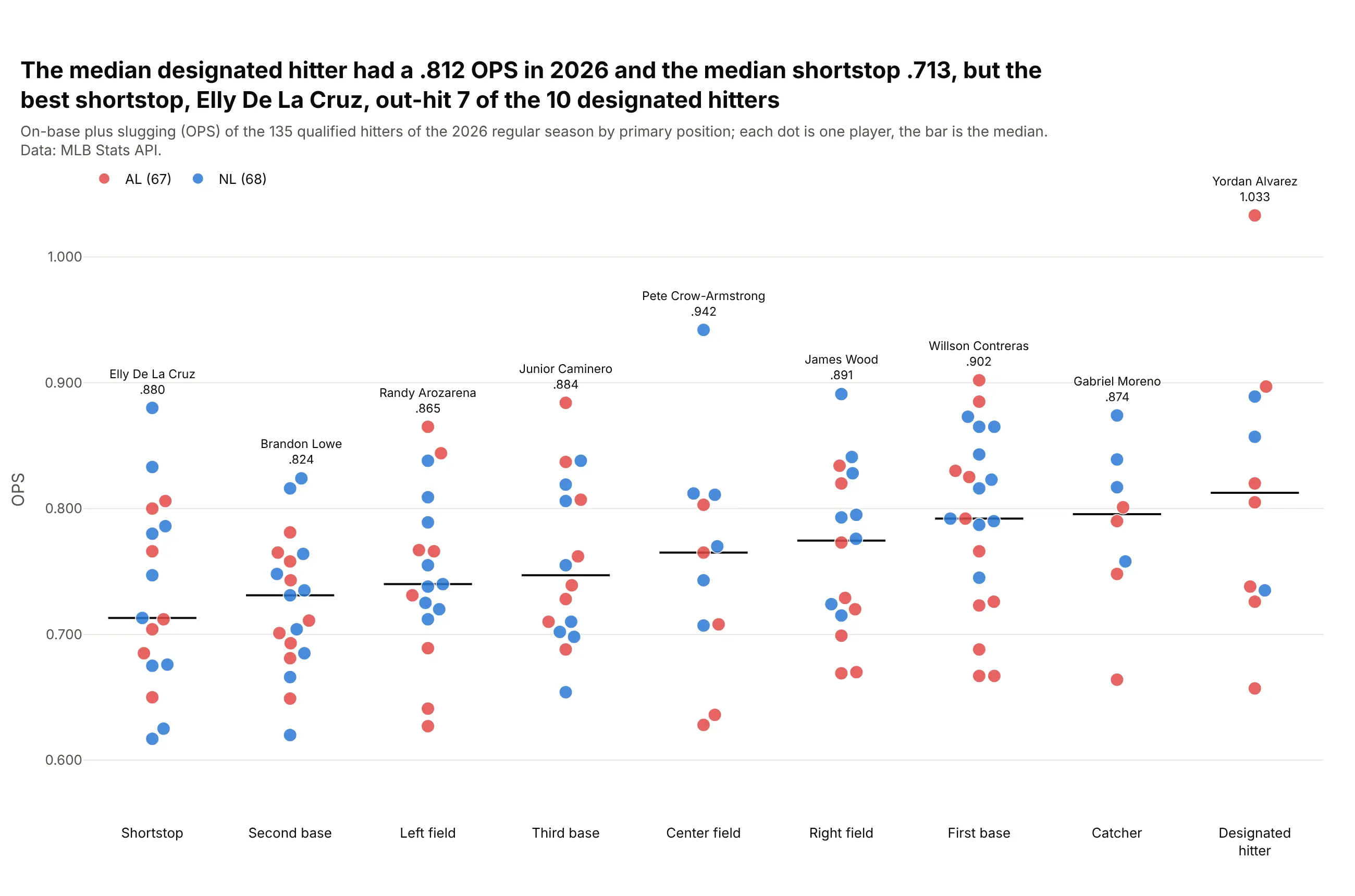
Vertical beeswarm of 135 qualified MLB hitters' 2026 OPS, one column per position sorted by median from shortstop (.713) to designated hitter (.812), dots colored by league, with the best hitter at each position labeled, led by Yordan Alvarez at 1.033

The median designated hitter had a .812 OPS in 2026 and the median shortstop .713, but the best shortstop, Elly De La Cruz (.880), out-hit 7 of the 10 designated hitters. Data: MLB Stats API, 2026 regular season.

Tip: for small groups (8 to 21 players), a vertical beeswarm shows every player where a box plot would invent quartiles.

Get the data from the MLB Stats API (season hitting stats, 2026, playerPool=qualified) and shape
it into a table (columns: player, team, league, position, ops).

Build a plotly vertical beeswarm: one column per position sorted by median OPS, y = OPS,
13 px markers colored by league, a median bar per column, the best hitter at each position labeled.

8. Open LLMs by size

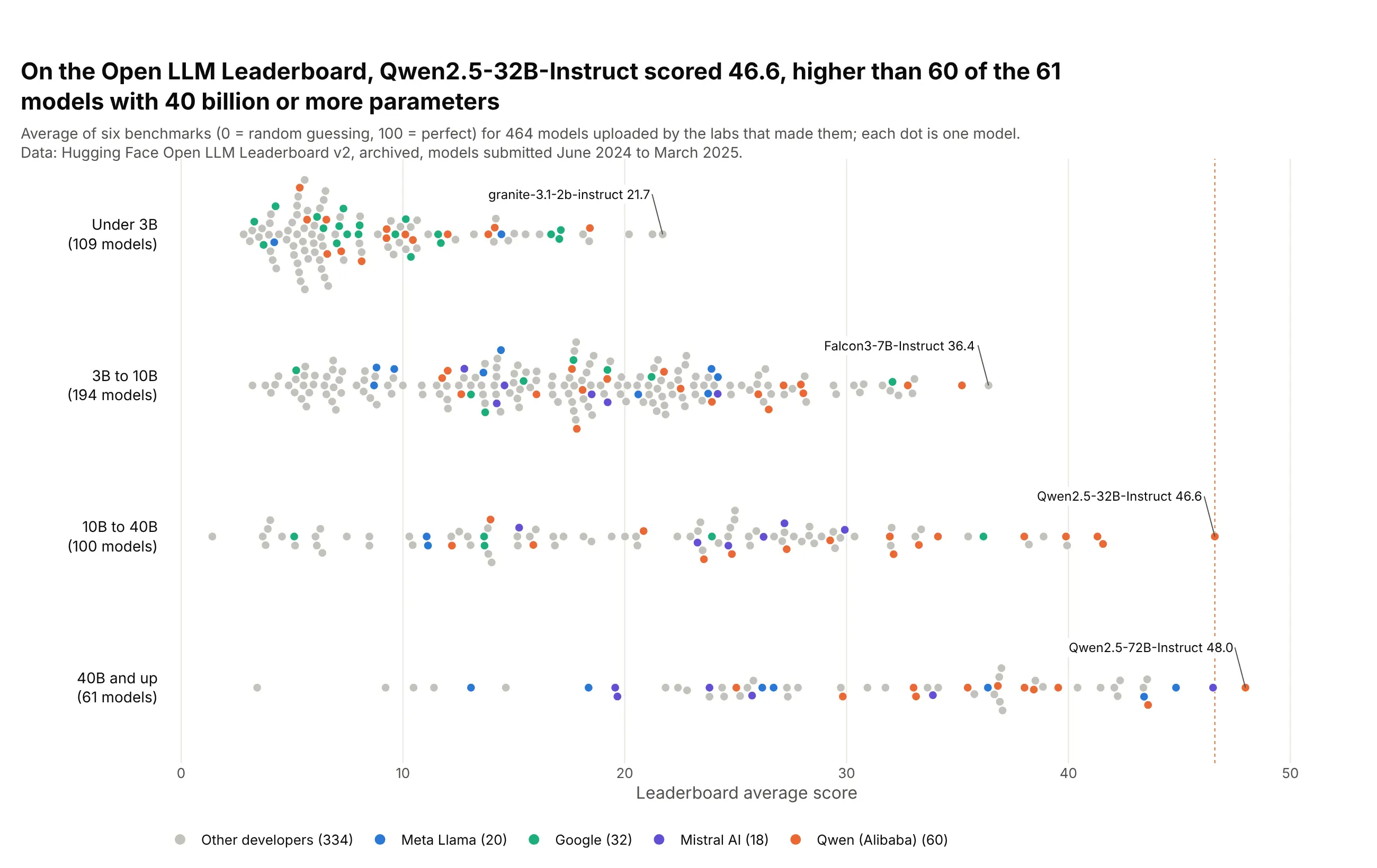
Beeswarm of 464 open language models' Open LLM Leaderboard scores in four rows by parameter count, with Qwen, Google, Meta and Mistral models in color; Qwen2.5-32B-Instruct at 46.6 sits past every 40B+ model but one

Qwen2.5-32B-Instruct scored 46.6 on the archived Open LLM Leaderboard, higher than 60 of the 61 models with 40 billion or more parameters. Size helps, but every row overlaps the next. Data: Hugging Face Open LLM Leaderboard v2, models submitted June 2024 to March 2025.

Tip: color four named developers and leave the other 334 models gray, so the families are easy to follow across rows.

Get the data from the Hugging Face Open LLM Leaderboard v2 dataset (open-llm-leaderboard/contents,
models flagged "Official Providers") and shape it into a table (columns: model, developer, params_b, average).

Build a plotly beeswarm: rows by size class (<3B, 3-10B, 10-40B, 40B+), x = average score,
8 px markers, Qwen, Google, Meta and Mistral in color and the rest gray, the best model per row labeled.

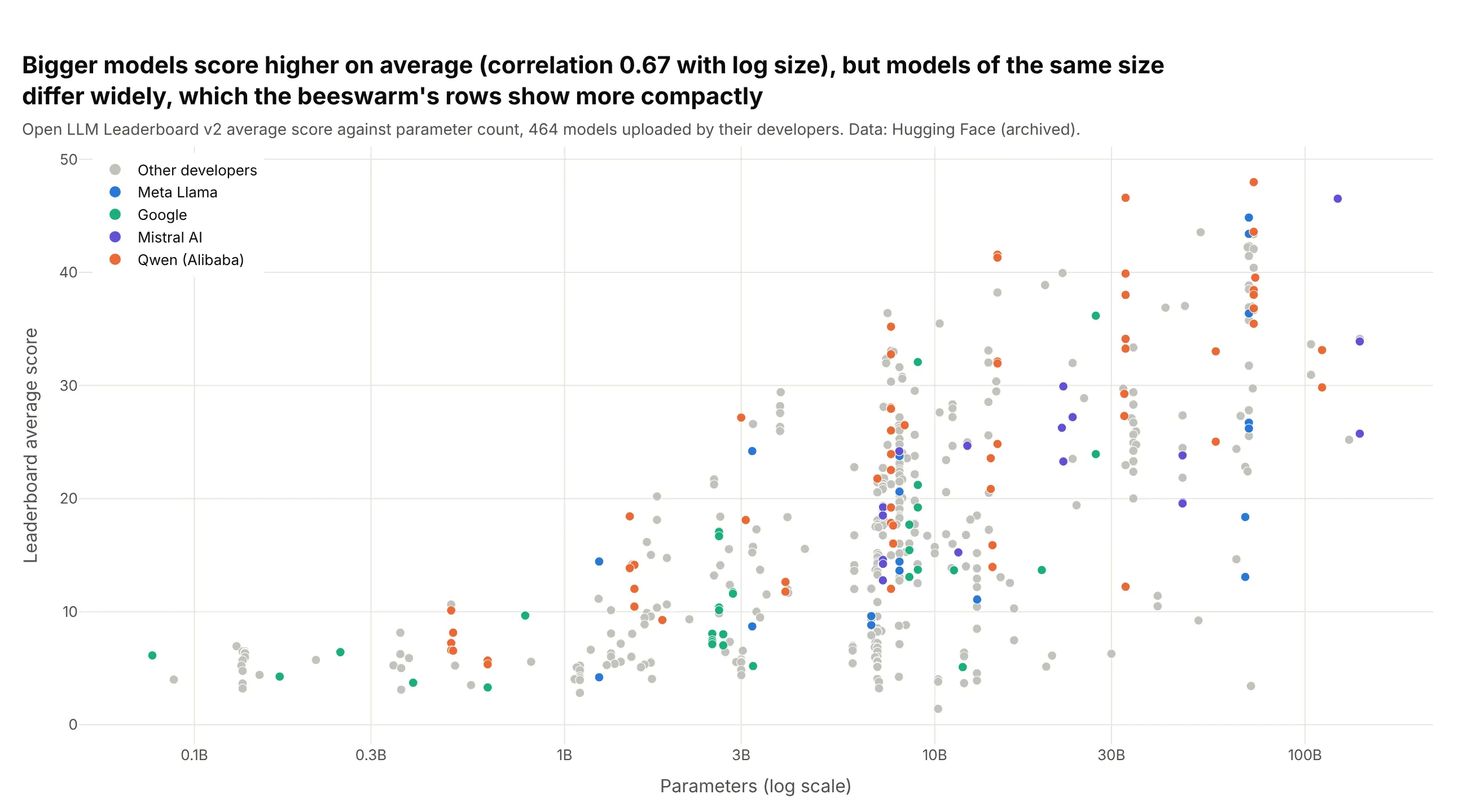
Another way to see it: a scatter plot against parameter count shows the trend (a 0.67 correlation with log size) but spreads the models thinly.

Scatter plot of 464 models' leaderboard scores against parameter count on a log axis, colored by developer

9. SHAP values of a machine learning model

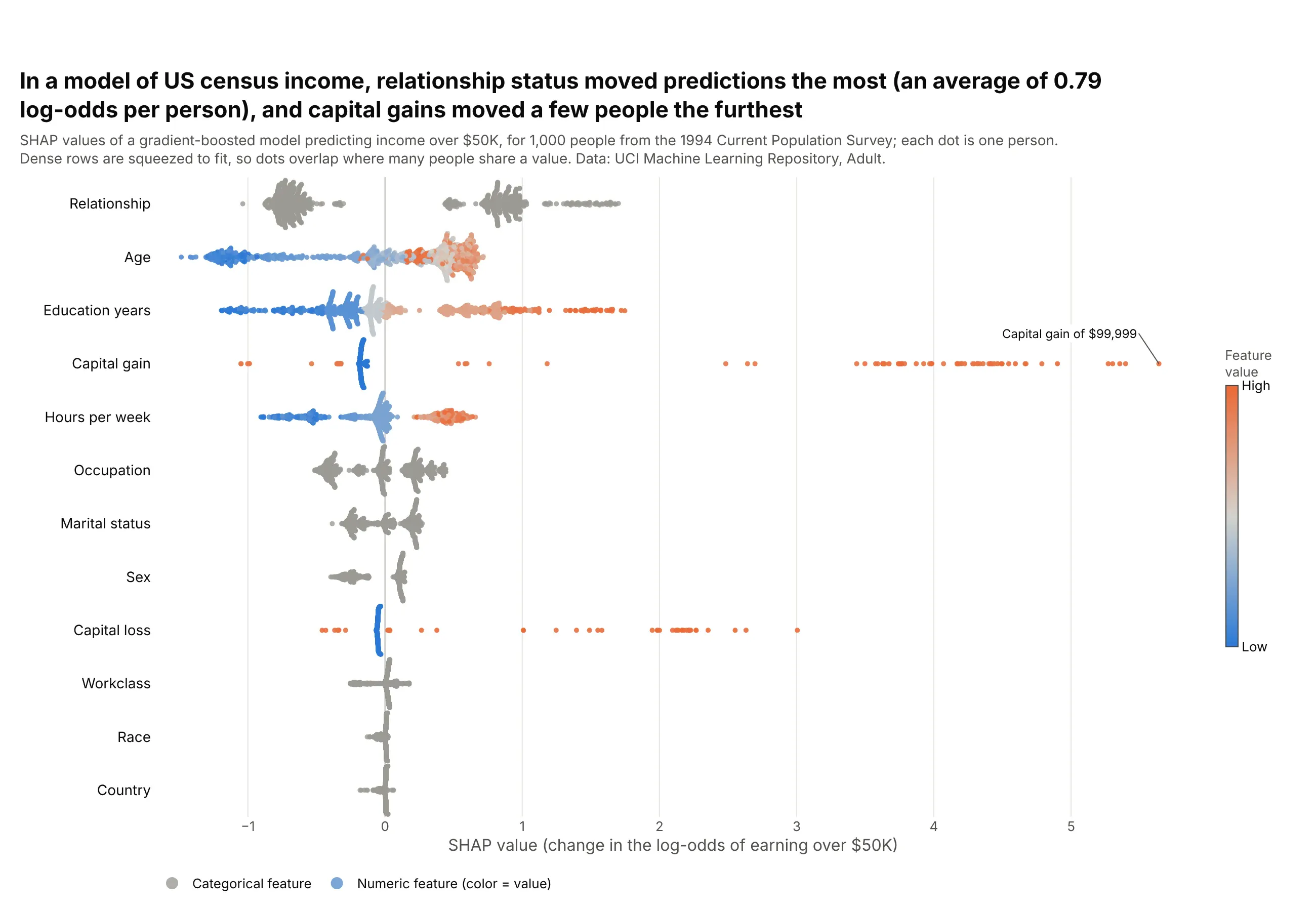
Beeswarm of SHAP values for 1,000 people in the UCI Adult census income data, one row per model feature sorted by mean absolute SHAP value, from relationship, age, education years and capital gain at the top to workclass, race and country at the bottom. Numeric features are blue for low values and orange for high; a capital gain of $99,999 has the largest value, about +5.6

The SHAP summary plot that data scientists use to explain a model is a beeswarm, with one row per feature and one dot per person. In a gradient-boosted model of the classic UCI Adult census income data, the relationship column moved predictions the most, by an average of 0.79 log-odds per person, and the few people with large capital gains were pushed furthest toward earning over $50K. Data: UCI Machine Learning Repository, Adult (1994 Current Population Survey), with SHAP values from the shap package.

Tip: squeeze each row to a fixed height, as shap.plots.beeswarm does, because hundreds of people with no capital gain share almost the same value and would otherwise stack into a tower.

Get the data from the UCI Machine Learning Repository's Adult dataset (adult.data),
fit a scikit-learn GradientBoostingClassifier for income over $50K, compute SHAP values with
shap.TreeExplainer for 1,000 random people, and shape them into a long table
(columns: person, feature, shap, value).

Build a plotly beeswarm: one row per feature sorted by mean absolute SHAP value, x = SHAP value,
numeric features colored from blue (low) to orange (high) by value and categorical ones gray,
a line at 0, and each row squeezed to a fixed height.