Chris Parmer

November 3, 2026

Strip Charts - A Complete Guide

TL;DR

A strip chart draws every value as a dot along one axis, usually one strip per group, and spreads tied values sideways with a little jitter so none hide behind another.
Strip charts are also known as strip plots, one-dimensional scatter plots, dot plots and jitter plots, and are similar to box plots, beeswarm plots and violin plots.
Use one for tens to a few thousand values per group, when you want readers to see every observation, the group sizes and the ties. For tens of thousands of points, use a histogram, a violin or an ECDF.
You can make a strip chart with Plotly in one line of code with px.strip, which draws each group as a box trace with the box hidden and the points jittered.
"Strip chart" also names the paper trace of a chart recorder, such as a seismograph. That meaning has its own section below, with a scrolling real-time version in Dash.

What is a strip chart?

Strip charts look like this:

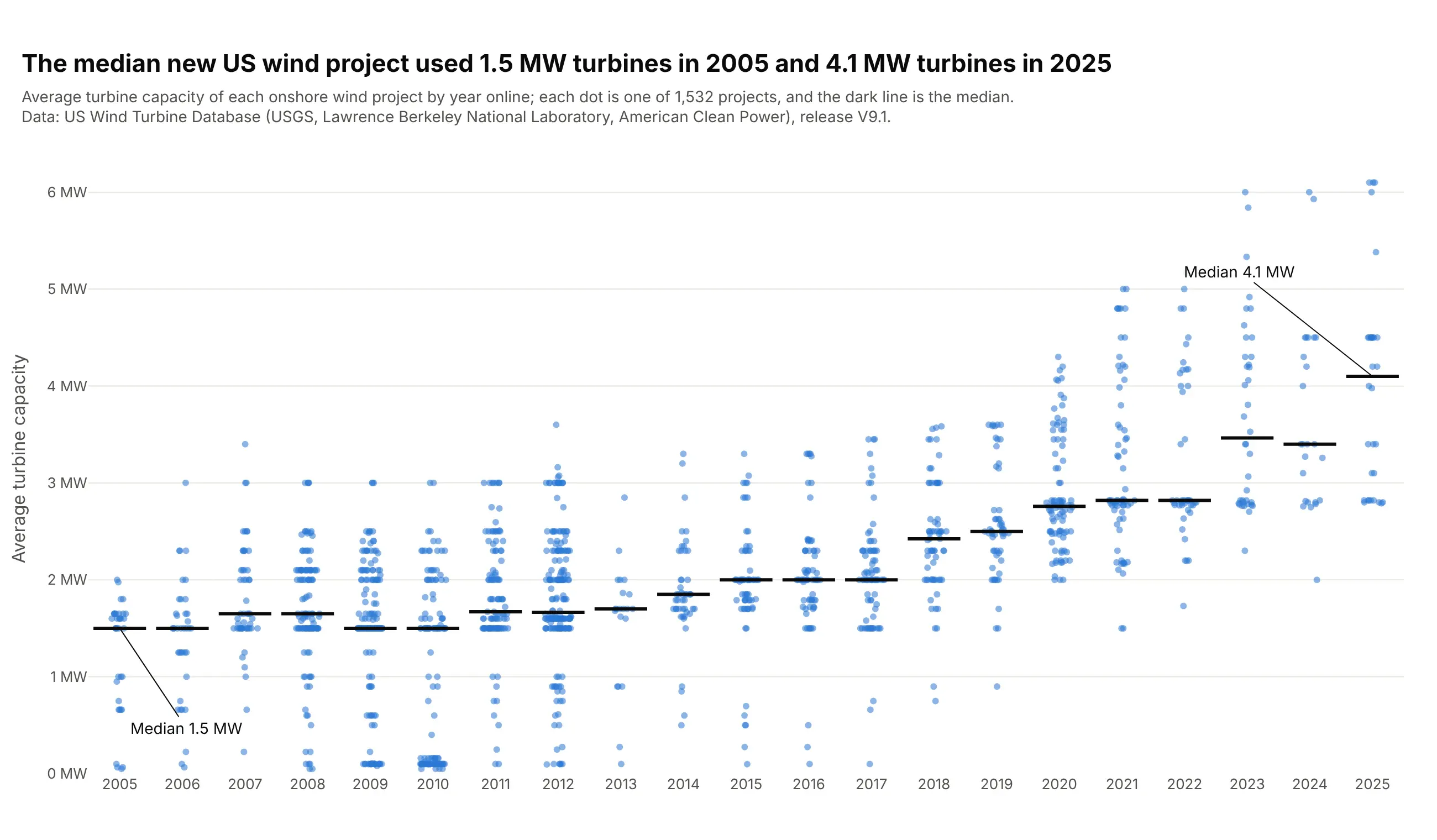
Strip chart of 1,532 US onshore wind projects by year online, 2005 to 2025, each dot one project at its average turbine capacity, with a dark median line per year rising from 1.5 MW in 2005 to 4.1 MW in 2025

Data: U.S. Wind Turbine Database (USGS, Lawrence Berkeley National Laboratory, American Clean Power), release V9.1.

How do you read a strip chart? In the example above, notice these things:

Each dot is one onshore US wind project, placed in the column for the year it came online and at the height of its turbines' average capacity.
Only the height carries data. The sideways spread inside a column is jitter, which moves dots apart so projects with the same value don't sit on top of each other.
Rows of dots at exactly the same height are projects that used the same turbine. 213 projects average exactly 1.5 MW, and 126 of them came online between 2009 and 2012.
The dark line is each year's median: 1.5 MW in 2005, 2.0 MW from 2015 to 2017 and 4.1 MW in 2025.
The number of dots is the number of projects, 192 in 2012 against 21 in 2013, which a box plot would hide. The cluster near zero in 2010 is 46 projects under 0.2 MW, mostly a single small turbine at a school, farm or wastewater plant.

It's often used for charts like these:

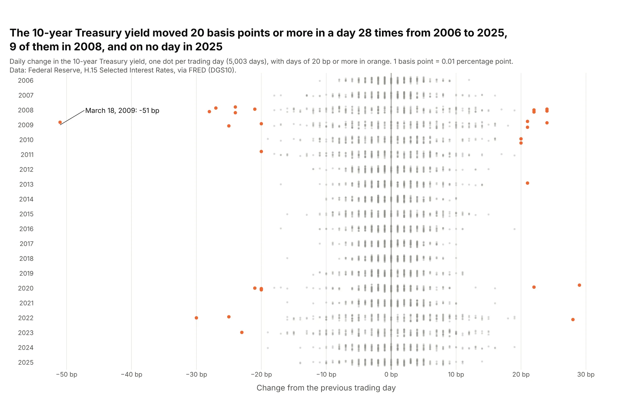
Strip chart of 5,003 daily changes in the 10-year Treasury yield from 2006 to 2025, one row per year, gray dots in vertical columns at whole basis points and 28 days of 20 bp or more in orange, the largest -51 bp on March 18, 2009

Volatility by year. The 10-year Treasury yield moved 20 basis points or more on 28 days from 2006 to 2025, 9 of them in 2008, and the width of each year's strip shows how calm or rough it was. Data: Federal Reserve H.15 via FRED (DGS10).

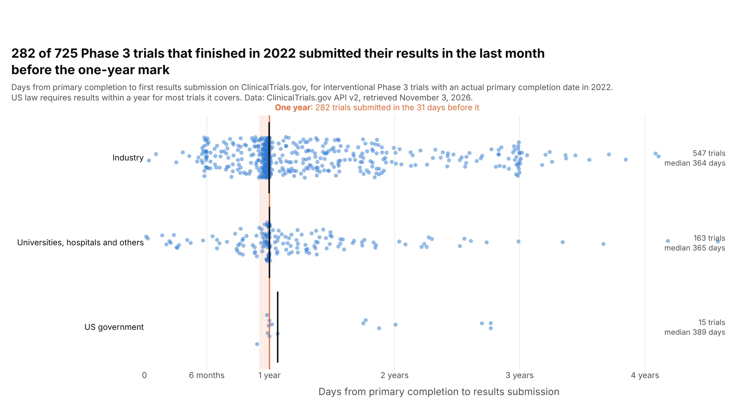
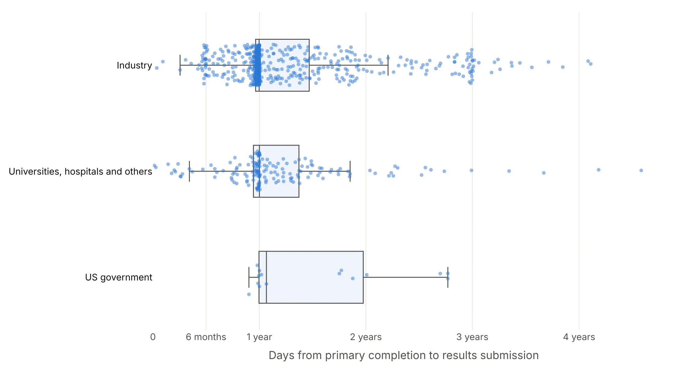
Strip chart of 725 Phase 3 trials that finished in 2022 by days from primary completion to results submission, one row per sponsor type, with a dense wall of dots just before the one-year line where 282 trials submitted in the last 31 days

Deadlines in clinical data. 282 of 725 Phase 3 trials that finished in 2022 submitted their results to ClinicalTrials.gov in the 31 days before the one-year mark, which shows as a wall of dots. Data: ClinicalTrials.gov API v2.

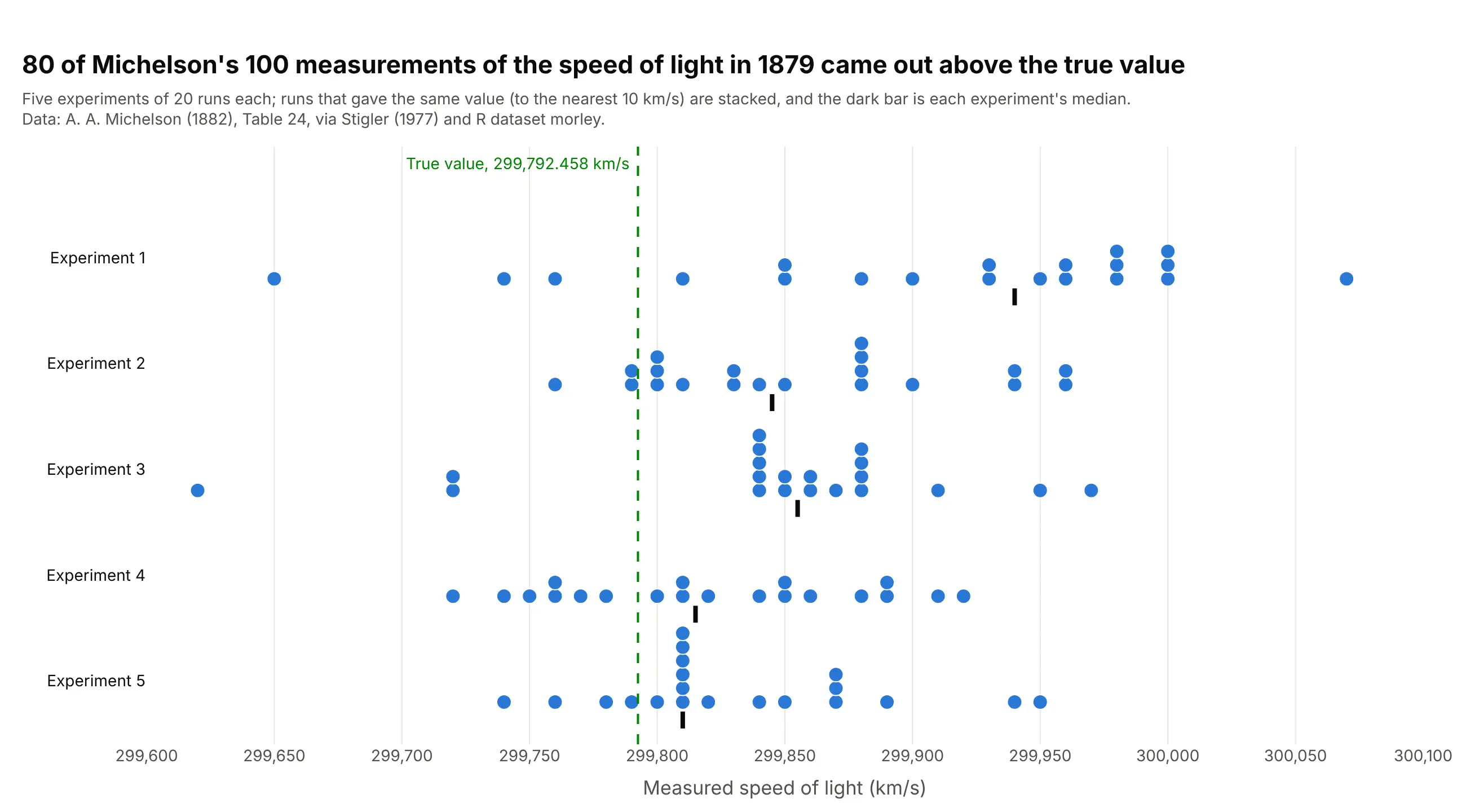
Michelson's 100 speed-of-light measurements from 1879, five rows of 20 runs with tied values stacked upward and a green dashed line at the true value of 299,792.458 km/s, to the left of 80 of the dots

Repeated measurements. 80 of Michelson's 100 measurements of the speed of light in 1879 came out above the true value, a bias the dots show against a reference line. Data: Michelson (1882) via Stigler (1977), R dataset morley.

A short history

Plotting each measurement as a dot along a scale is one of the simplest statistical charts. R's graphics package has a stripchart() function that draws "one dimensional scatter plots (or dot plots)" and calls them "a good alternative to boxplots when sample sizes are small". Chambers, Cleveland, Kleiner and Tukey's 1983 book Graphical Methods for Data Analysis discussed jitter, the small offset that separates tied values (as cited by Wicklin), and Python's seaborn library added the same chart as stripplot (Waskom 2021). The chart reads well because it shows values as positions on a common scale, the most accurate encoding in Cleveland and McGill's experiments (1984).

Strip chart recorders and real-time strip charts

Some people who search for "strip chart" mean the paper chart of a strip chart recorder, a long strip of paper that moves under a pen at a steady speed so the pen draws a signal over time. Wikipedia's chart recorder article describes an early one that Charles Babbage built into a railway dynamometer car in 1838 or 1839, and seismographs and ECG machines are familiar modern examples. This is a seismogram of the July 29, 2025 Kamchatka earthquake, recorded in Albuquerque, New Mexico:

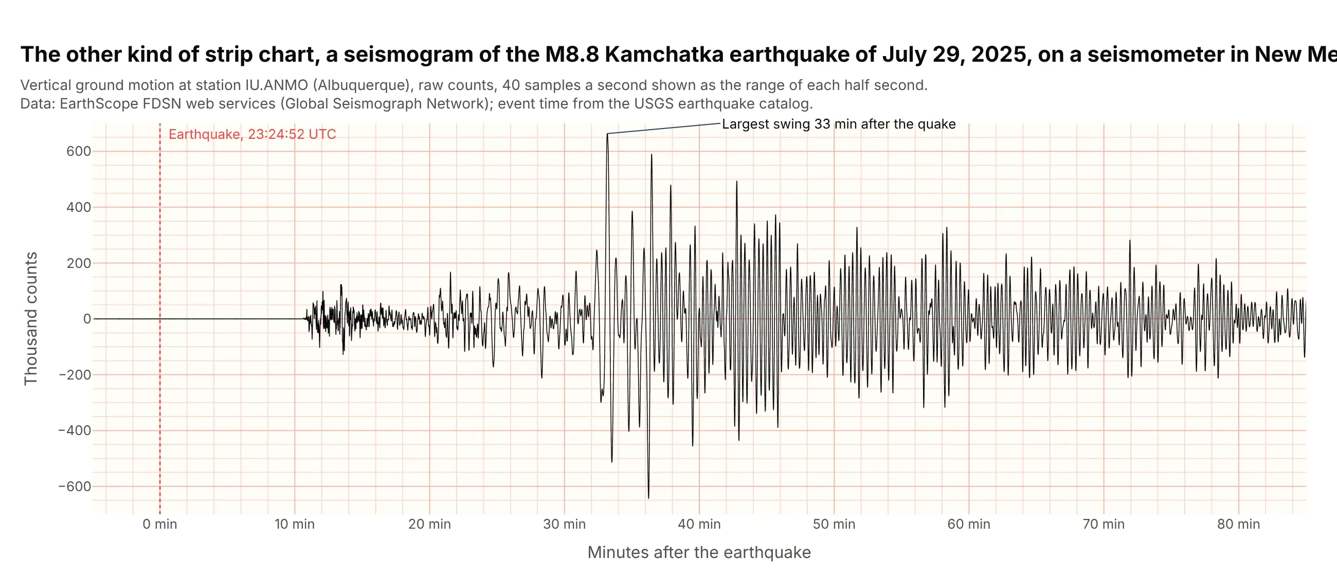
Seismogram of the M8.8 Kamchatka earthquake of July 29, 2025, from station IU.ANMO in Albuquerque, drawn as a black line on pink recorder-style grid paper: flat until about 11 minutes after the quake, then growing swings with the largest 33 minutes after it

Data: EarthScope FDSN web services, Global Seismograph Network station IU.ANMO; event time from the USGS earthquake catalog.

On a screen, the same idea is a scrolling line chart that keeps the latest few thousand points. In Dash, a dcc.Interval fires a callback every few hundred milliseconds, and the callback returns new points to the graph's extendData property, whose third item caps how many points stay on screen:

import pandas as pd
import plotly.graph_objects as go
from dash import Dash, Input, Output, dcc, html

data = pd.read_csv("seismogram.csv")  # minutes_after_origin, counts
STEP, WINDOW = 120, 3000

fig = go.Figure(go.Scatter(x=[], y=[], mode="lines", line=dict(color="black", width=1)))
fig.update_layout(template="simple_white", yaxis_range=[-700, 700])

app = Dash()
app.layout = html.Div([dcc.Graph(id="strip", figure=fig), dcc.Interval(id="tick", interval=200)])

@app.callback(Output("strip", "extendData"), Input("tick", "n_intervals"))
def add_samples(n):
    chunk = data.iloc[(n or 0) * STEP:((n or 0) + 1) * STEP]
    new = dict(x=[chunk.minutes_after_origin.tolist()], y=[(chunk.counts / 1000).tolist()])
    return new, [0], WINDOW  # [updateData, traceIndices, maxPoints]

app.run()

This replays the recorded quake. In your own app, replace the chunk = ... line with a read from your sensor, message queue or database. The rest of this guide is about the statistical strip chart.

Alternatives to a strip chart

Here's the same Phase 3 trial data drawn six ways. Some are better for the question, some worse, some just different:

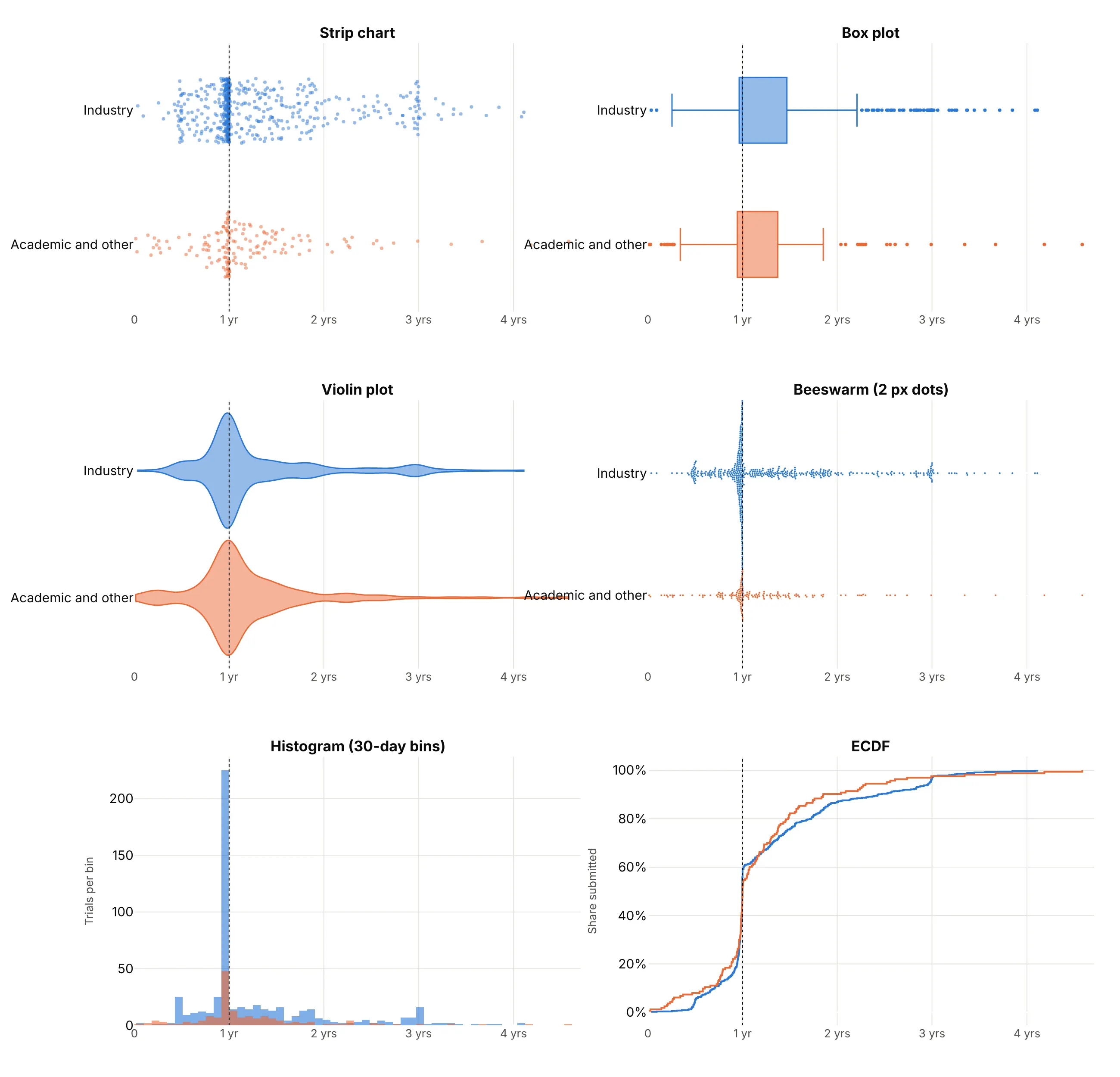
The 710 industry and academic Phase 3 trials drawn six ways on the same axis of days to results submission: a strip chart, box plots, violins, a beeswarm whose column at one year runs off the panel, a histogram with a tall bar just before one year, and ECDF curves that jump at one year

Box plot (better for many groups). Five numbers per group compare well side by side, but the wall of submissions just before one year disappears inside the box, and so does the fact that industry has more than three times as many trials.
Violin plot (better for big n). The smoothed outline shows the peak at one year and scales to any number of points, but it smears the sharp edge into a gentle bump and you can't hover a single trial.
Beeswarm plot (worse here). It places every dot without overlap, which is better than jitter for a few hundred points, but the trials that submitted in the last weeks before the deadline pile into a column taller than the row.
Histogram (better for exact counts). With 30-day bins the bar just before one year shows the pile-up as a count you can read off the axis, though the names and the exact days are gone.
ECDF (better for "what share by when"). The near-vertical jump at one year is the deadline, and you can read that 58% of trials had submitted by then, but the curve takes practice to read.

How to make a strip chart

With AI

ChatGPT, Claude Code, GitHub Copilot, Cursor and other AI tools are excellent at writing Plotly code. Name Plotly in the prompt, and say what should happen to tied values and what reference lines you want:

Make a plotly strip chart from wind_projects.csv (columns: project, state, year, turbines, turbine_mw).

- Use px.strip with x = year (as categories, in order) and y = turbine_mw, one strip per year.
- Jitter 0.85, 6 px markers at 0.55 opacity, project and state in the hover text.
- A short dark line at each year's median, and the first and last medians labeled.
- Fixed width and height, the y axis in MW from 0, and a title that states the takeaway.
- Check: print the median per year and the number of projects per year.

With Plotly Studio

Plotly Studio is a desktop app where you point an AI at a dataset and it builds charts and a Dash app around your questions. Ask for a strip chart the same way:

Show a strip chart of days from primary completion to results submission for each Phase 3 trial, one row per sponsor type, every trial as a jittered dot with its NCT ID on hover, a vertical line at 365 days and the median of each row marked.

Make a strip chart in Python or JavaScript

This is the code AI tools write under the hood. In Python, px.strip makes the chart in one line of code, and the Plotly strip chart documentation covers color and faceting:

import pandas as pd
import plotly.express as px

df = pd.read_csv("wind_projects.csv").sort_values("year")  # project, state, year, turbine_mw

fig = px.strip(df, x="year", y="turbine_mw", hover_name="project",
               labels={"year": "", "turbine_mw": "Average turbine size (MW)"})
fig.update_traces(jitter=0.85, marker=dict(size=6, opacity=0.55))
fig.update_xaxes(type="category")  # one strip per year

# a short line at each year's median
for i, (year, median) in enumerate(df.groupby("year").turbine_mw.median().items()):
    fig.add_shape(type="line", x0=i - 0.4, x1=i + 0.4, y0=median, y1=median, line=dict(color="black", width=3))
fig.show()

px.strip returns a figure with one box trace per color, with boxpoints="all" and the box made invisible. Plotly's jitter is repeatable, so the same data gives the same picture every time, and it spreads points further where values are dense. To show the box as well, use go.Box(..., boxpoints="all") with a visible line.

In JavaScript, plotly.js draws the same thing from a box trace:

<div id="chart"></div>
<script src="https://cdn.plot.ly/plotly-4.1.1.min.js"></script>
<script>
  // Michelson's 1879 speed-of-light runs, experiments 4 and 5 (km/s minus 299,000; R dataset morley)
  const expt4 = [890, 810, 810, 820, 800, 770, 760, 740, 750, 760, 910, 920, 890, 860, 880, 720, 840, 850, 850, 780];
  const expt5 = [890, 840, 780, 810, 760, 810, 790, 810, 820, 850, 870, 870, 810, 740, 810, 940, 950, 800, 810, 870];

  const strip = (values, name) => ({
    type: "box", x: values.map(v => v + 299000), name: name, orientation: "h",
    boxpoints: "all", jitter: 0.6, pointpos: 0,                 // every point, spread sideways, centered
    fillcolor: "rgba(0,0,0,0)", line: {width: 0}, hoveron: "points",  // hide the box itself
    marker: {size: 10, color: "#2a78d6", opacity: 0.7}
  });

  Plotly.newPlot("chart", [strip(expt4, "Experiment 4"), strip(expt5, "Experiment 5")], {
    width: 800, height: 320, showlegend: false, margin: {l: 110, r: 20, t: 20, b: 50},
    xaxis: {title: {text: "Speed of light (km/s)"}, tickformat: ","},
    shapes: [{type: "line", x0: 299792.458, x1: 299792.458, yref: "paper", y0: 0, y1: 1,
              line: {color: "#008300", dash: "dash"}}]           // the true value
  });
</script>

Share it

Every Plotly chart has a Share chart button (the cloud icon in its toolbar) that uploads it to Plotly Cloud and gives you a link. Only you can see it until you change its visibility.

For a live app, put the chart in a Dash app and publish it with the Plotly Cloud CLI. Coding agents can run these commands for you:

pip install "dash[cloud]"
plotly user login
plotly app publish

If your data has to stay in your own cloud or data center, publish to Dash Enterprise instead.

Dos and don'ts

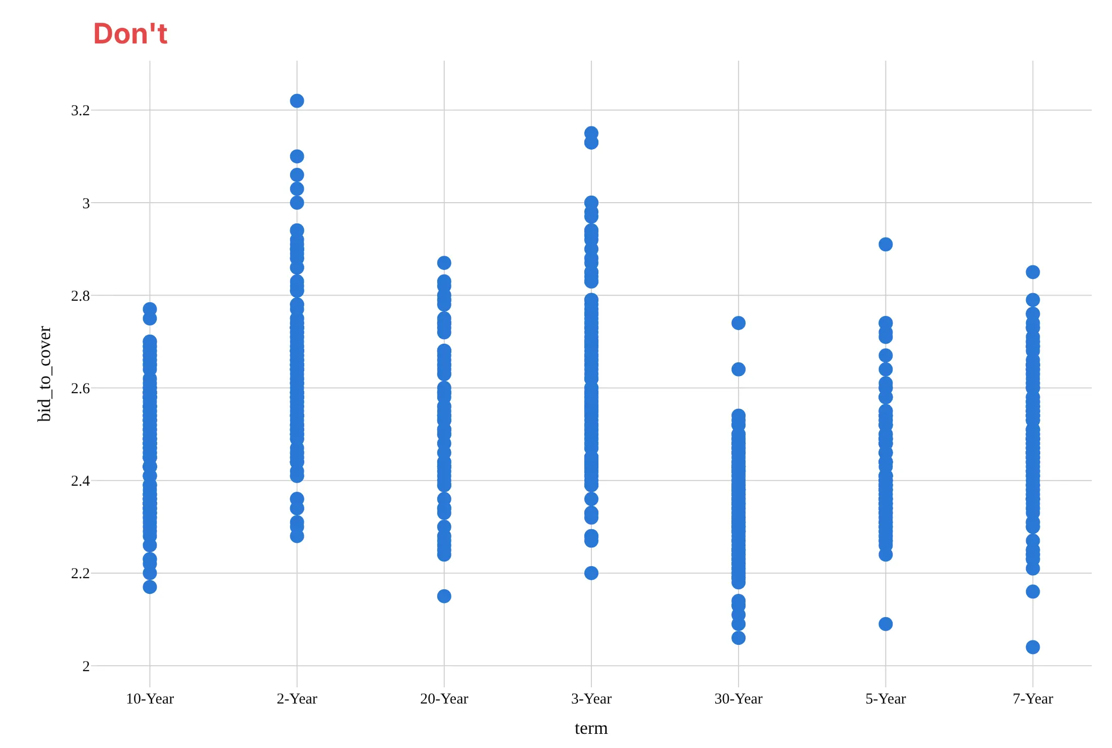
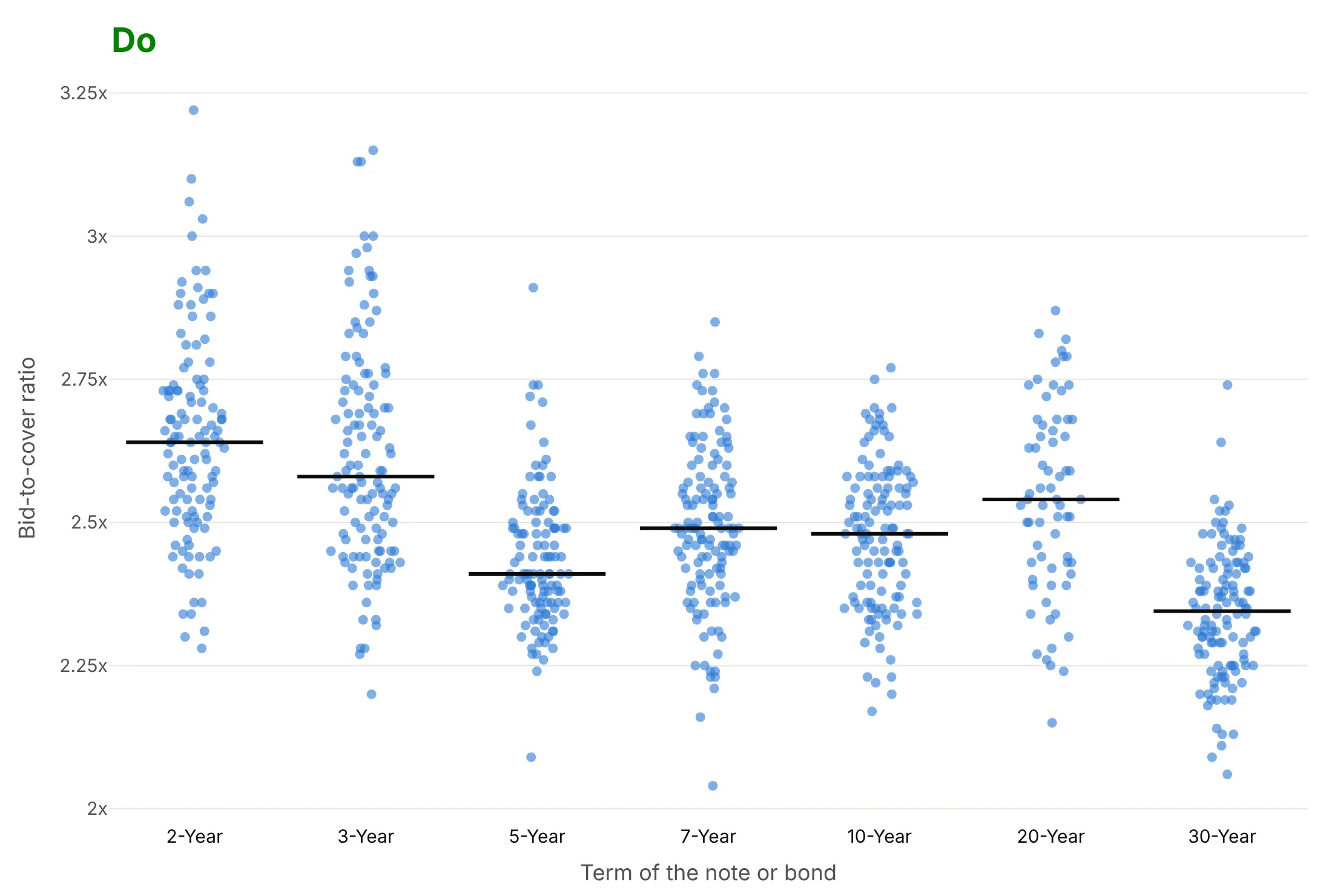
Most of the work in a published strip chart is handling ties, ordering the groups and marking a reference. Here are 788 Treasury auctions both ways, in the same color.

Don't draw the dots without jitter so auctions with the same ratio hide behind each other, use big opaque markers, leave the terms in alphabetical order (10-Year before 2-Year), or use a default serif font and raw column names as axis titles:

788 Treasury auctions' bid-to-cover ratios as solid columns of large overlapping blue dots, terms in alphabetical order from 10-Year to 7-Year, a serif font and the axis titles term and bid_to_cover

Do jitter the dots, make them small and partly transparent so dense areas look darker, order the terms by maturity, mark each median and format the axis:

The same 788 auctions as a jittered strip chart with small semi-transparent dots, terms in order from 2-Year to 30-Year, a dark median line per term and the axis labeled Bid-to-cover ratio

Choose how to handle ties

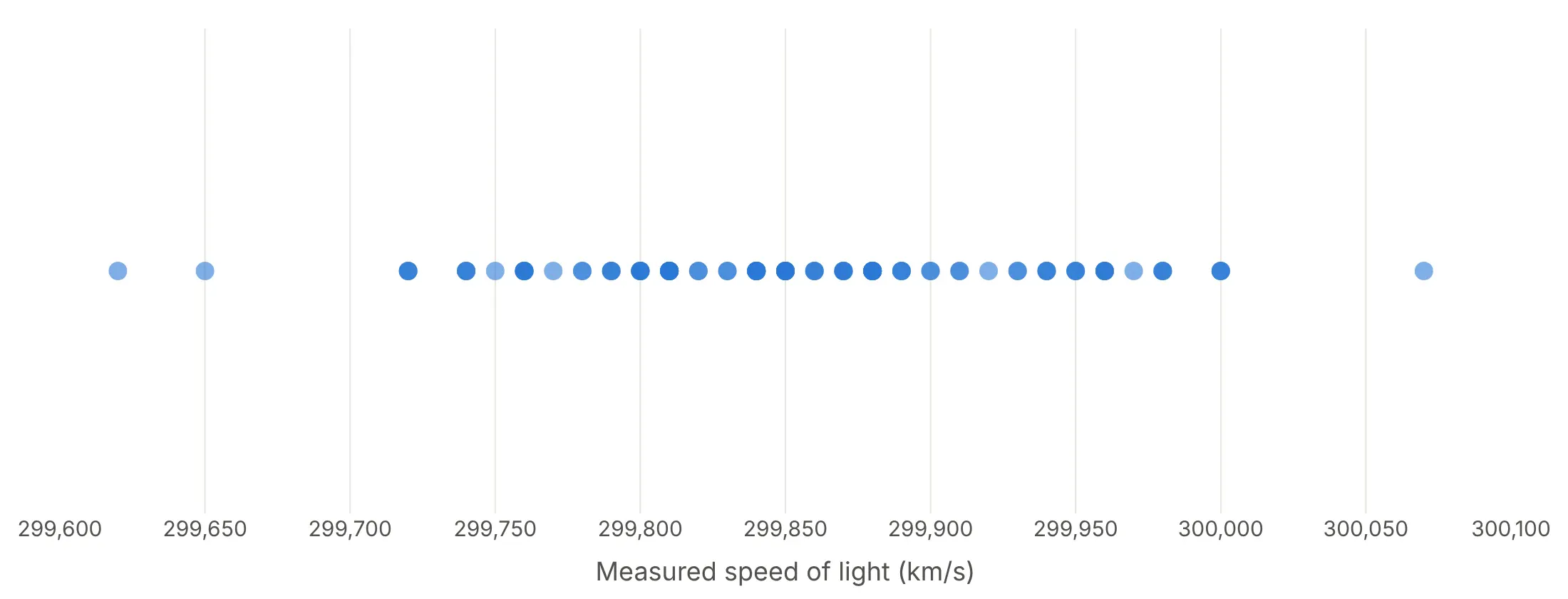
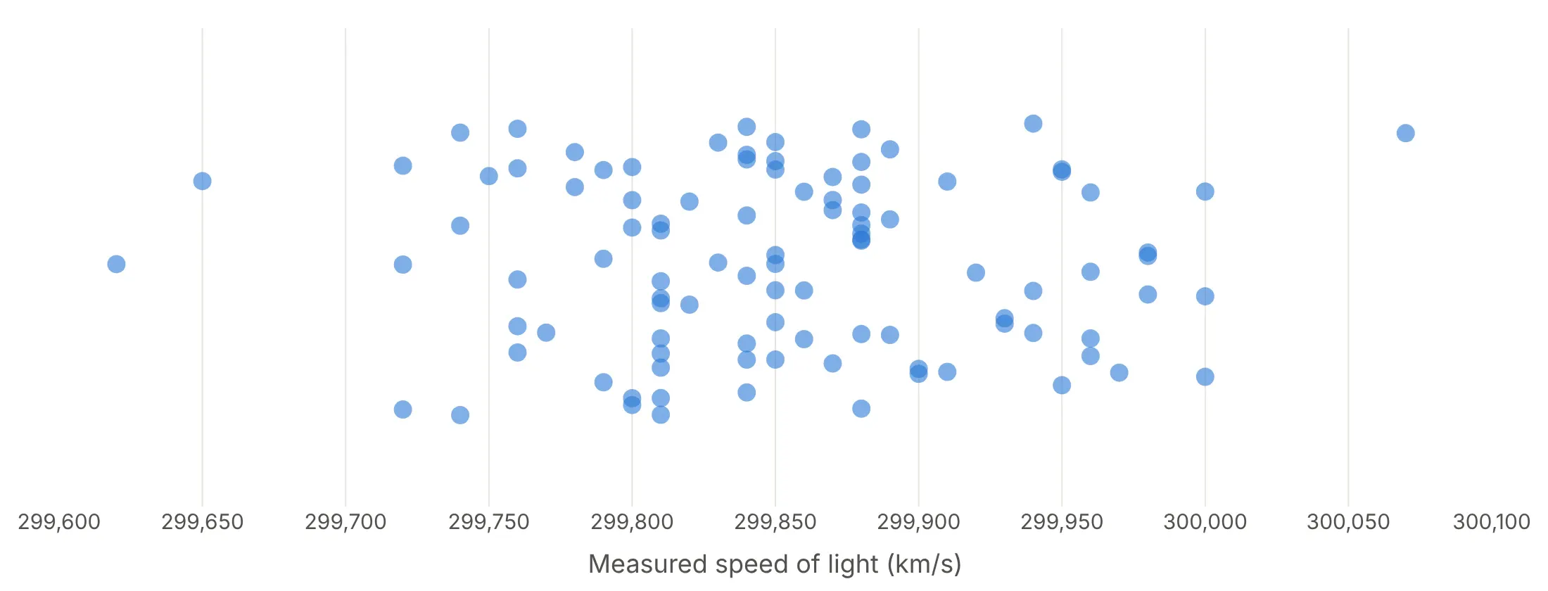
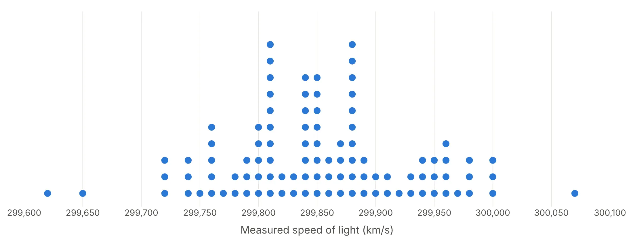
R's stripchart() offers three methods for values that repeat, and they show Michelson's 100 runs, which have only 30 distinct values, very differently.

Overplot. Every run at the same value lands on the same spot, so 100 measurements look like 30 dots.

Michelson's 100 runs in one strip with no offset: 30 dots in a single row, ties hidden

Jitter. Random vertical offsets separate the ties. It works for any data, and px.strip jitters by default.

The same 100 runs with random vertical jitter, every run visible

Stack. Ties pile up in columns, which turns the strip into a dot histogram. Use it for rounded data like this, where the stacks are exact counts.

The same 100 runs stacked: columns of dots at 299,810 and 299,880 km/s are 10 dots tall

Add a box behind the dots

A light box plot behind the dots adds the quartiles without hiding a single trial. In Plotly this is one go.Box trace with boxpoints="all" and a visible line:

The 725 Phase 3 trials as jittered dots with a light box plot behind each sponsor type

Checklist

Jitter or stack tied values, so every observation is visible.
Use small, partly transparent markers above a few hundred points per group.
Order groups by something meaningful (time, maturity, median), not alphabetically.
Mark each group's median or mean with a short line, and add reference lines (a deadline, a true value, zero).
Put each point's name in the hover text, and label the few points the story needs.
Write a title that states the takeaway.

Don't

Use a strip chart for tens of thousands of points per group; switch to a histogram, violin or ECDF.
Read meaning into the jitter direction; it carries no data.
Use so much jitter that neighboring groups' dots run into each other.

Options to customize

A strip chart in Plotly is px.strip or a go.Box trace with its points shown, so these are the options that matter most. The full lists are in the px.strip reference and the box trace reference.

px.strip(x=..., y=...): the value column on one axis and the group column on the other; swap them for horizontal strips.
color, stripmode="group": a second grouping drawn side by side within each group, as in the guinea pig example below.
facet_col, facet_row: small multiples of strip charts.
jitter: the width of the sideways spread, from 0 (none) to 1 (the full width of the group).
pointpos: where the points sit relative to the group center; 0 centers them.
boxpoints="all" (go.Box): shows every point; with line_width=0 and a transparent fillcolor it hides the box.
marker.size, marker.opacity: 10-12 px and opaque for small groups, 3-6 px and 0.3-0.6 opacity for thousands of points.
hover_name, hover_data, hovertemplate: the item's name and details on hover.
category_orders or xaxis.categoryarray: the order of the groups.
add_shape, add_vline, add_hline, add_vrect: median lines, deadlines, true values and shaded windows.
xaxis.type="log": a log value axis for data that spans orders of magnitude; shapes take data values, annotations take log10 of them.
go.Scattergl: WebGL markers with jitter you compute yourself, for more than about 50,000 points.

More strip chart examples

Eight more strip charts built from real public data, each with its source, the technique that makes it work and a prompt to rebuild it. Several use the small textbook experiments that strip charts are best known for, from R's built-in datasets.

1. The 1905 sleep trial behind Student's t-test

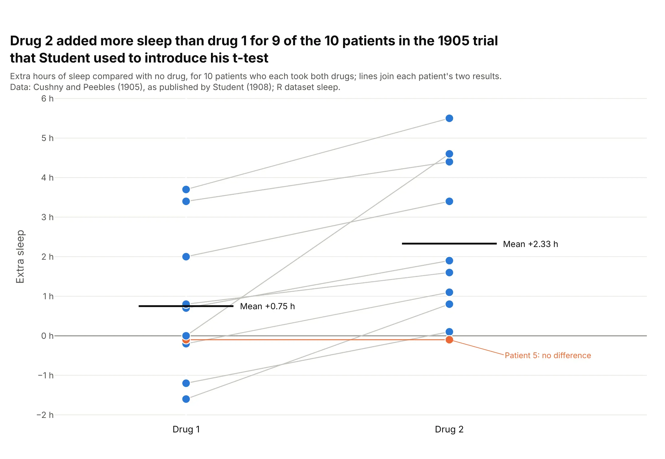
Strip chart of 10 patients' extra hours of sleep on two drugs, one column per drug, with a gray line joining each patient's two values; drug 2 is higher for 9 patients and equal for patient 5, shown in orange, and the means are +0.75 h and +2.33 h

Drug 2 added more sleep than drug 1 for 9 of 10 patients, and the mean difference was 1.58 hours. Student used these data in the 1908 paper that introduced his t-test. Data: Cushny and Peebles (1905) via Student (1908), R dataset sleep.

Tip: when each subject is measured twice, join the two dots with a light line so the pairing shows.

Get the data from R's built-in sleep dataset (Cushny and Peebles 1905, as used by Student 1908) and
shape it into a table (columns: patient, drug, extra_hours).

Build a plotly strip chart: one column per drug, 14 px dots, a gray line joining each patient's two
values, a short dark bar at each drug's mean, and the patient with no difference in orange.

2. Demand at US Treasury auctions

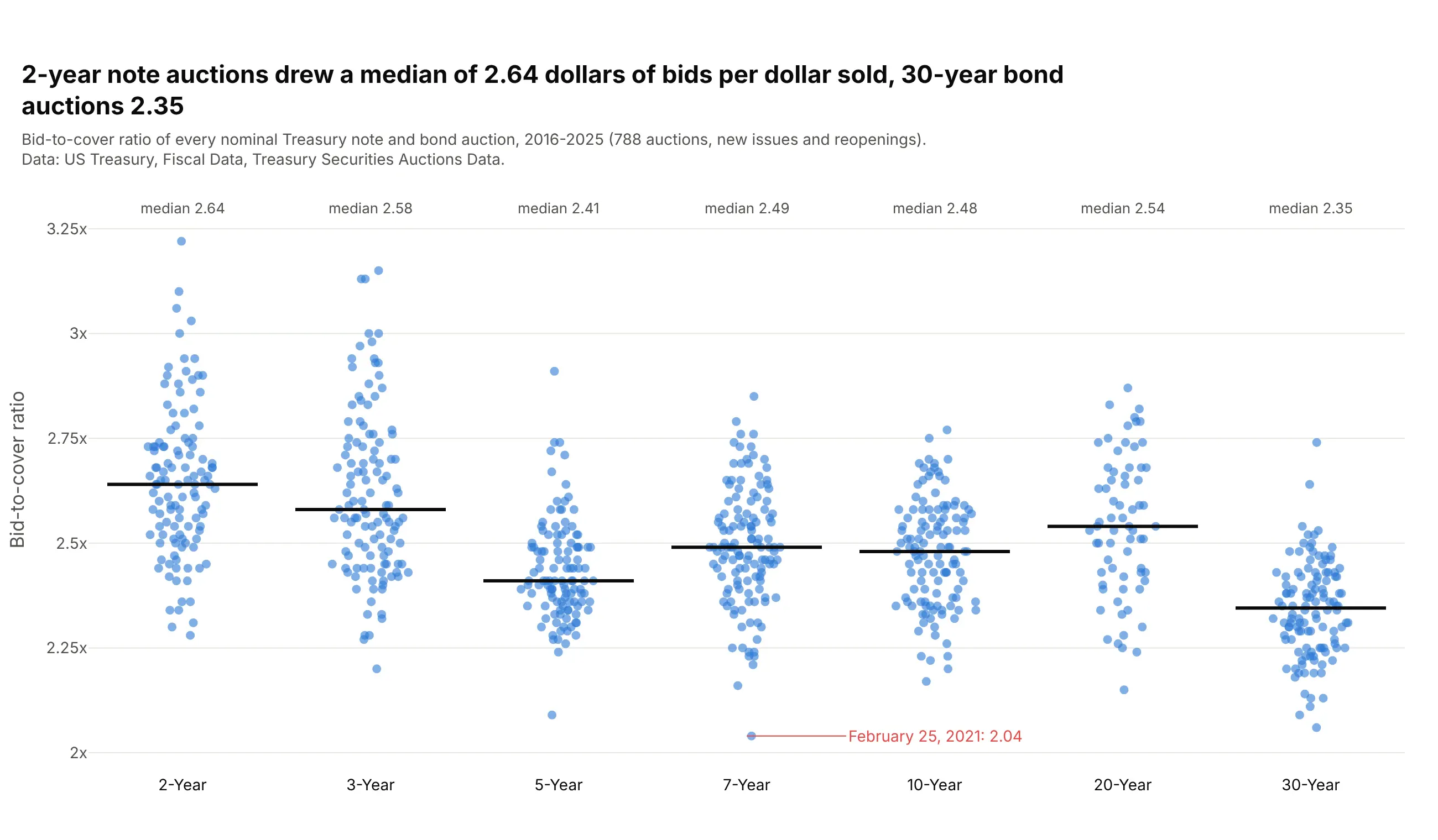
Strip chart of 788 Treasury note and bond auctions' bid-to-cover ratios from 2016 to 2025, one column per term from 2-Year to 30-Year with medians from 2.64 to 2.35, and the weakest auction, a 7-year on February 25, 2021 at 2.04, labeled

2-year note auctions drew a median of 2.64 dollars of bids per dollar sold from 2016 to 2025, and 30-year bonds 2.35. The weakest of 788 auctions was a 7-year note on February 25, 2021, at 2.04. Data: US Treasury, Fiscal Data, Treasury Securities Auctions Data.

Tip: with about 120 points per group, a strip shows the single weak auctions that a box plot would fold into a whisker.

Get the data from the US Treasury's Fiscal Data API (Treasury Securities Auctions Data, auctions_query),
nominal notes and bonds auctioned 2016-2025, and shape it into a table (columns: auction_date, term,
years, offering_bn, bid_to_cover).

Build a plotly strip chart: one column per term in order of maturity, jitter 0.9, 8 px dots at 0.6 opacity,
a median line and label per term, and the lowest auction labeled with its date.

3. Electricity per person in 195 countries

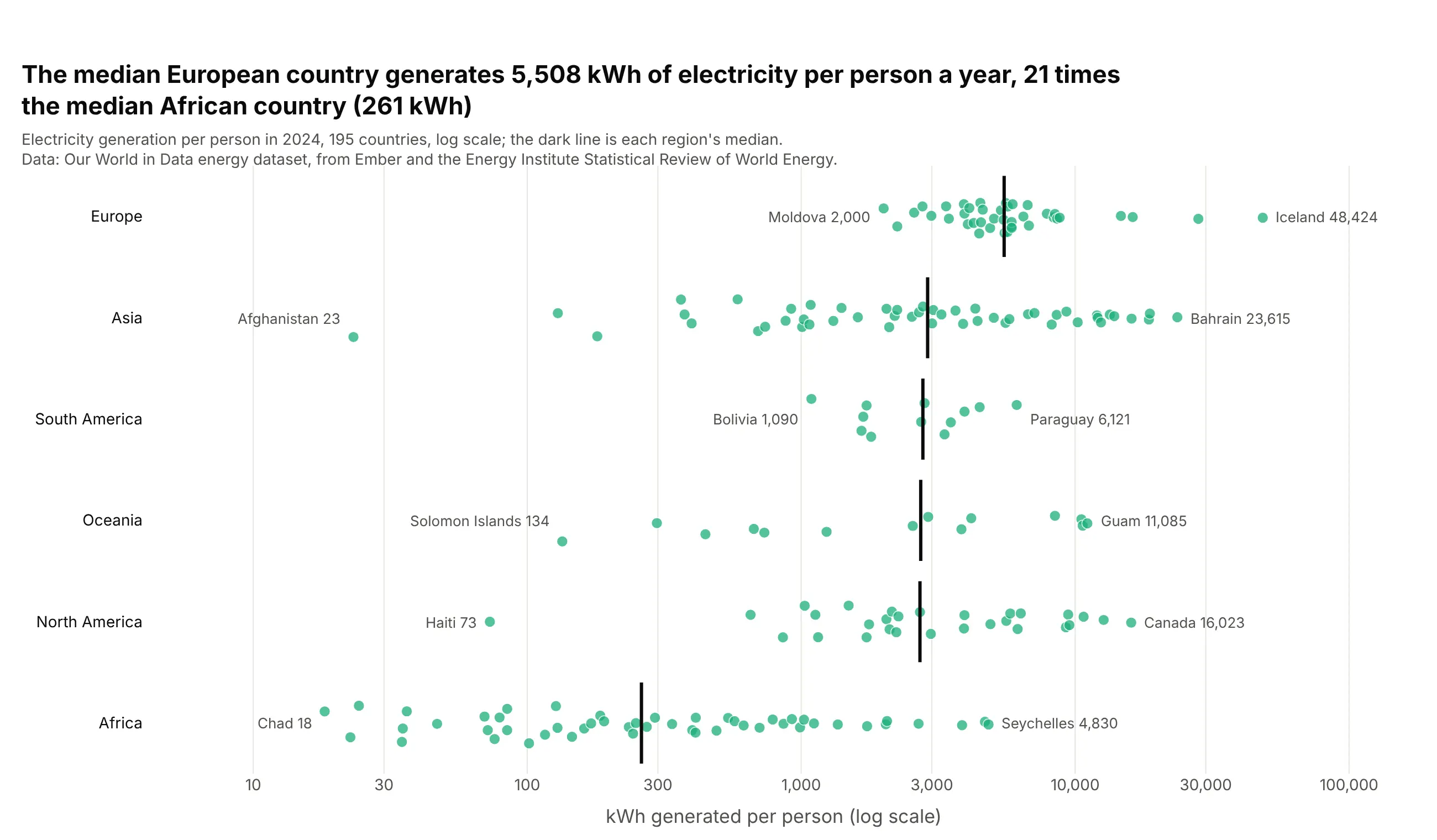
Strip chart of 195 countries' electricity generation per person in 2024 on a log axis, one row per region sorted by median from Europe (5,508 kWh) to Africa (261 kWh), with the lowest and highest country of each region labeled, from Chad at 18 kWh to Iceland at 48,424

The median European country generated 5,508 kWh of electricity per person in 2024, 21 times the median African country (261 kWh). Iceland, at 48,424 kWh, generates about 2,700 times as much per person as Chad (18 kWh). Data: Our World in Data, from Ember and the Energy Institute.

Tip: use a log axis when values span orders of magnitude, and label only each row's lowest and highest country.

Get the data from Our World in Data's energy dataset (github.com/owid/energy-data, from Ember and the
Energy Institute), year 2024, countries only, with OWID's world regions, and shape it into a table
(columns: country, region, kwh_per_person).

Build a plotly strip chart: one row per region sorted by median, x = kwh_per_person on a log axis,
a median tick per row, and the lowest and highest country in each region labeled.

4. Ten years of WTI crude oil prices

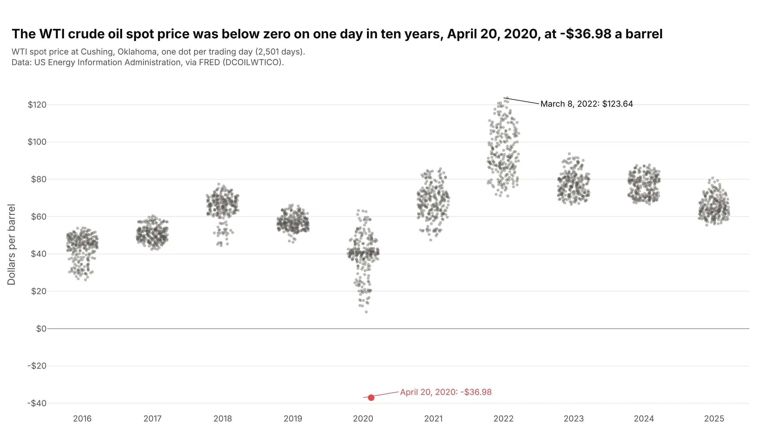
Strip chart of 2,501 daily WTI spot prices from 2016 to 2025, one column per year in gray, with a single red dot far below zero on April 20, 2020 at -$36.98 and the March 8, 2022 high of $123.64 labeled

The WTI spot price was below zero on one day in ten years, April 20, 2020, at -$36.98 a barrel. One strip per year shows each year's range and leaves that day on its own. Data: US EIA via FRED (DCOILWTICO).

Tip: draw the outlier as its own trace in a strong color, after the gray crowd, so it sits on top.

Get the data from the US EIA's daily WTI spot price at Cushing, Oklahoma (FRED series DCOILWTICO),
2016-2025, and shape it into a table (columns: date, year, price).

Build a plotly strip chart: one column per year, 5 px gray dots at 0.4 opacity, the one negative day
as a separate red trace with a label, the highest price labeled, and a line at $0.

5. How old Nobel laureates are when they win

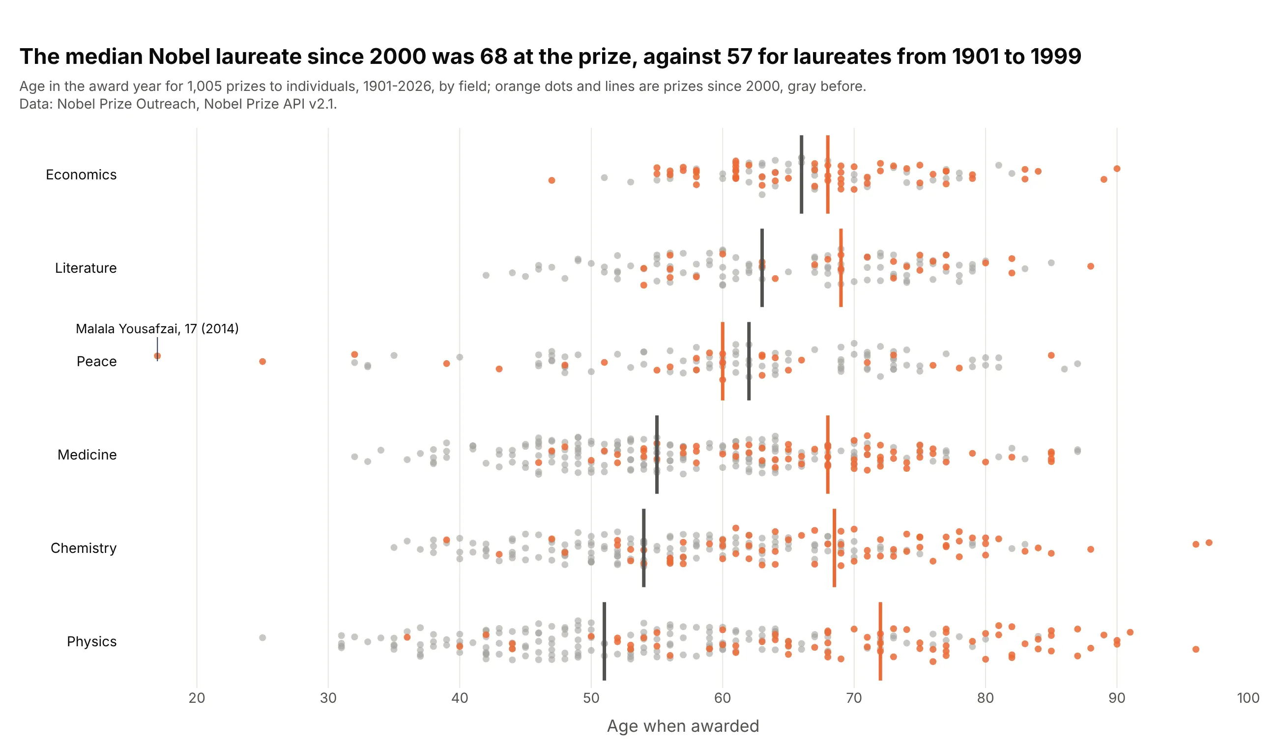
Strip chart of 1,005 Nobel prizes to people from 1901 to 2026 by age at the award, one row per field, prizes since 2000 in orange and earlier ones in gray, with orange median lines to the right of the gray ones in every field except Peace; Malala Yousafzai at 17 is labeled

The median Nobel laureate since 2000 was 68 when the prize was awarded, against 57 from 1901 to 1999. In physics the median went from 51 to 72. Data: Nobel Prize API v2.1.

Tip: color an era instead of a category, and draw a median line per era, so one chart answers "has this changed?".

Get the data from the Nobel Prize API v2.1 (api.nobelprize.org/2.1/laureates, people only) and shape
it into a table with one row per prize (columns: name, category, year, birth_year, age).

Build a plotly strip chart: one row per category sorted by median age, prizes since 2000 in orange on
top of earlier ones in gray, a median line for each era, and the youngest laureate labeled.

6. Thirty years of Central Park daily highs

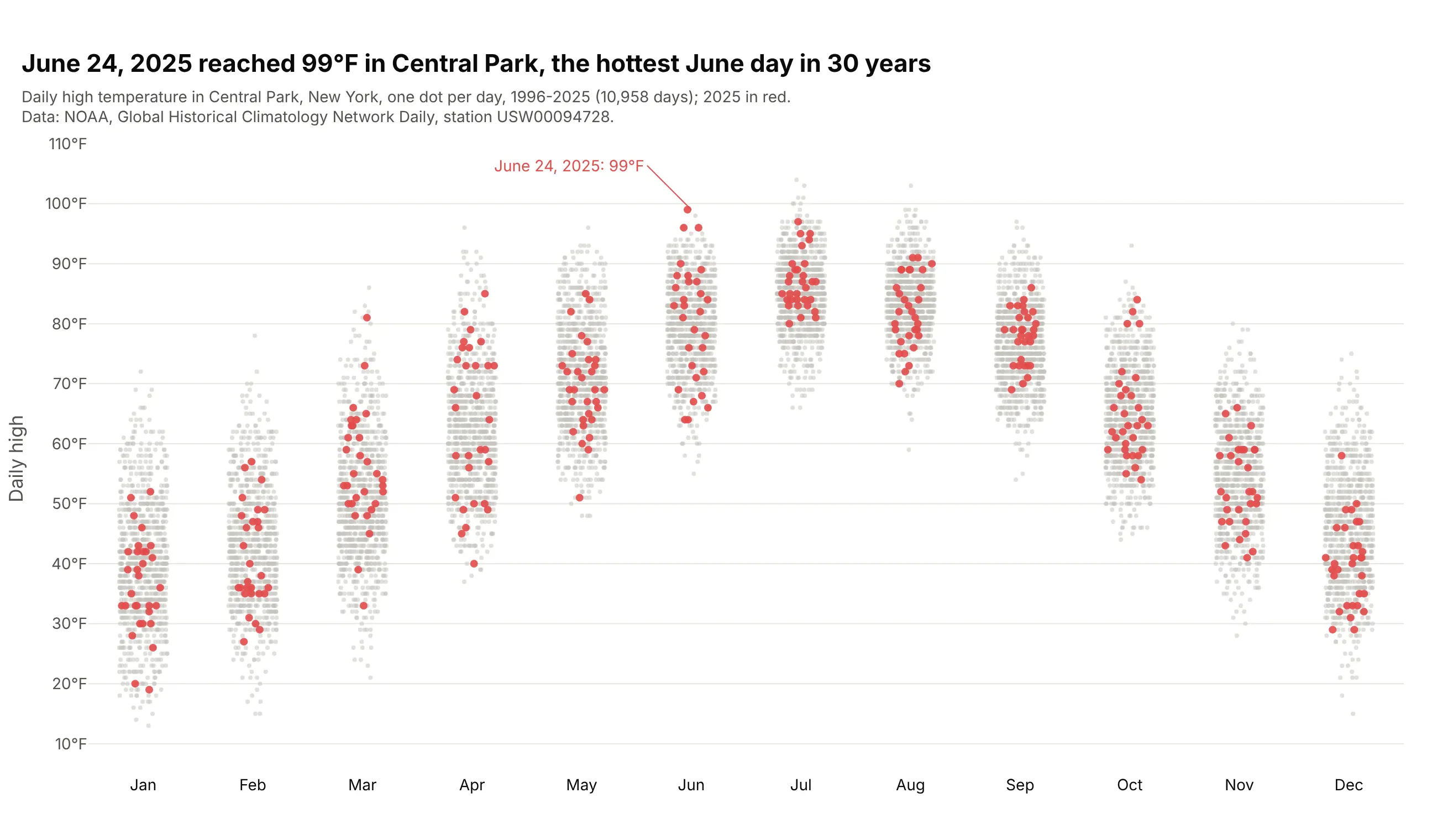
Strip chart of 10,958 daily high temperatures in Central Park from 1996 to 2025, one column per month in light gray, 2025's days in red on top, and June 24, 2025 at 99°F labeled as the hottest June day in the 30 years

June 24, 2025 reached 99°F in Central Park, the hottest June day from 1996 to 2025. Drawing one year on top of the other 29 shows where each day falls against history. Data: NOAA GHCN-Daily, station USW00094728.

Tip: with about 900 dots per month, use 4 px light gray markers for the history and bigger colored ones for the year in question.

Get the data from NOAA's Global Historical Climatology Network Daily file for station USW00094728
(Central Park, New York), daily TMAX 1996-2025, and shape it into a table (columns: date, year, month,
tmax_f).

Build a plotly strip chart: one column per month, 1996-2024 as 4 px gray dots, 2025 as 7 px red dots
on top, and the 2025 day that set a 30-year monthly record labeled.

7. Vitamin C dose response in guinea pigs

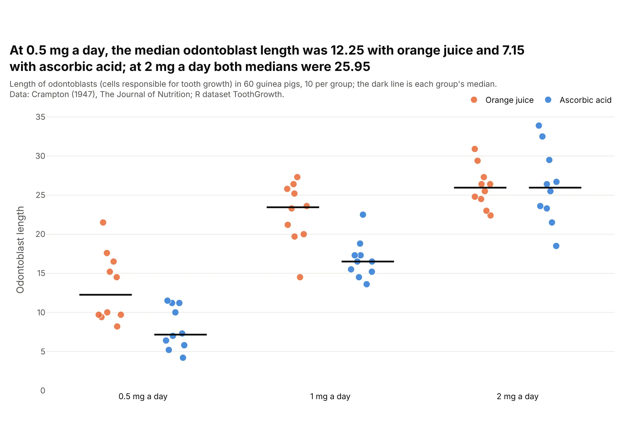
Strip chart of 60 guinea pigs' odontoblast lengths at three vitamin C doses, orange juice in orange and ascorbic acid in blue side by side within each dose, with medians of 12.25 and 7.15 at 0.5 mg a day and 25.95 for both at 2 mg a day

At 0.5 mg of vitamin C a day, the median odontoblast length was 12.25 with orange juice and 7.15 with ascorbic acid, and at 2 mg a day both were 25.95. With 10 animals per group, every one is visible. Data: Crampton (1947), R dataset ToothGrowth.

Tip: px.strip(..., color="supplement", stripmode="group") puts the two delivery methods side by side within each dose.

Get the data from R's built-in ToothGrowth dataset (Crampton 1947, The Journal of Nutrition) and
shape it into a table (columns: length, supplement, dose_mg).

Build a plotly strip chart with px.strip: x = dose, y = length, color = supplement with
stripmode="group", 12 px dots, and a short dark median line for each of the six groups.

8. R's own example: a honeybee repellent experiment

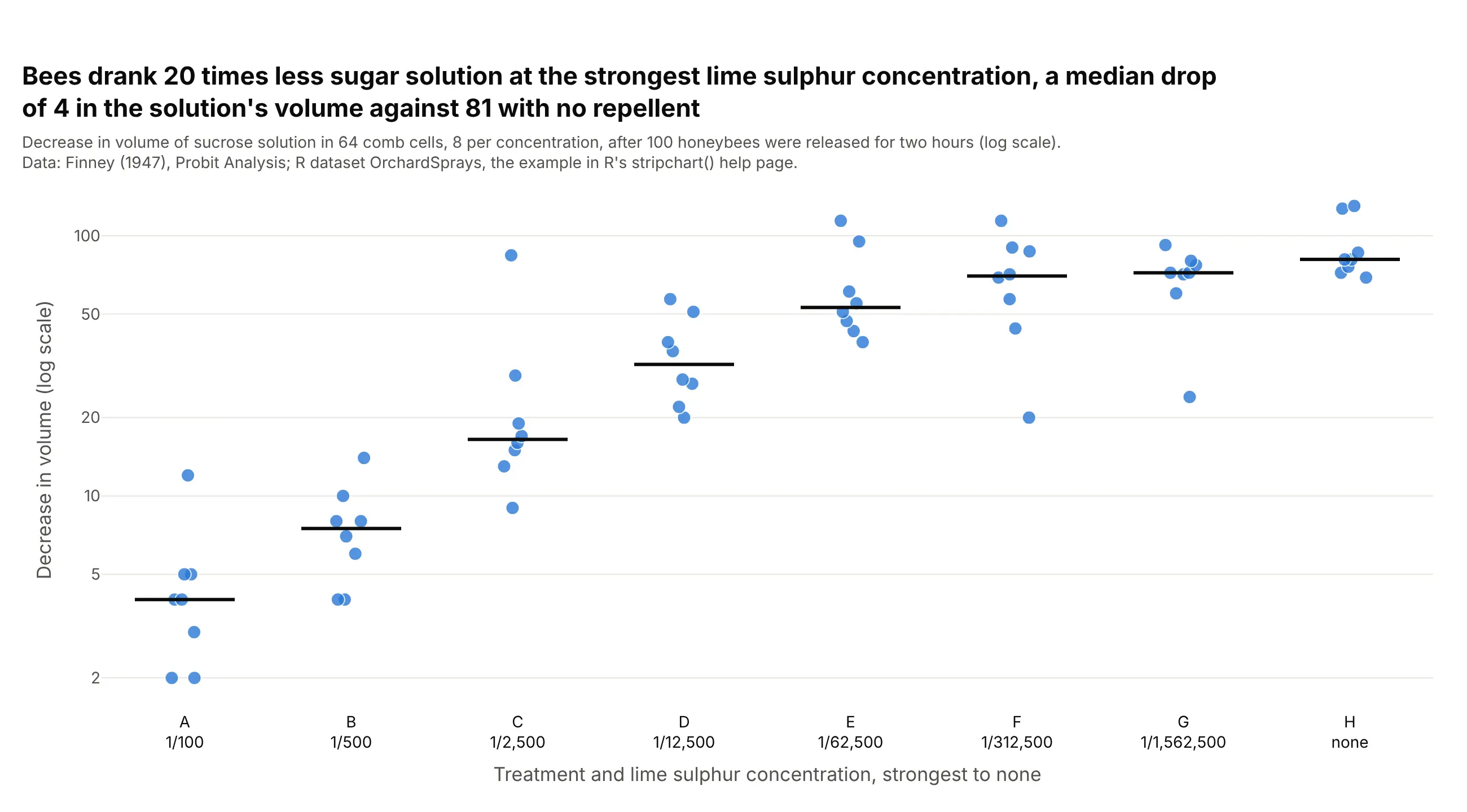
Strip chart of 64 comb cells in eight vertical strips by lime sulphur concentration from 1/100 to none, on a log axis, with median lines rising from 4 at the strongest concentration to 81 with no repellent

Bees drank 20 times less sugar solution at the strongest lime sulphur concentration, a median drop in volume of 4 against 81 with no repellent. This is the dataset R's stripchart() help page draws, vertical and on a log scale. Data: Finney (1947), Probit Analysis, R dataset OrchardSprays.

Tip: with 8 values per group, use big markers and light jitter, and a log axis when the groups differ by a factor of 20.

Get the data from R's built-in OrchardSprays dataset (Finney 1947, a Latin square experiment with
honeybees) and shape it into a table (columns: treatment, concentration, decrease).

Build a plotly strip chart: one vertical strip per treatment from A (1/100) to H (none), y = decrease
on a log axis, 12 px dots with light jitter, and a short dark median line per treatment.