Bubble Charts - A Complete Guide

TL;DR

• A bubble chart is a scatter plot whose markers are sized by a third number, so each bubble shows three values: x, y and area. Color can add a fourth.
• Bubble charts are also known as bubble plots, and are similar to scatter plots and proportional symbol maps.
• Use one when the size of each item changes how you read the relationship, such as countries by population, companies by market value or power plants by capacity.
• Size bubbles by area, not diameter, or a value 6 times bigger looks 36 times bigger. px.scatter(size=...) does this for you, and with go.Scatter you set sizemode="area".
• Any coding agent can make one with Plotly in a minute. In Python it's px.scatter(df, x=..., y=..., size=...).

What is a bubble chart?

Bubble charts look like this:

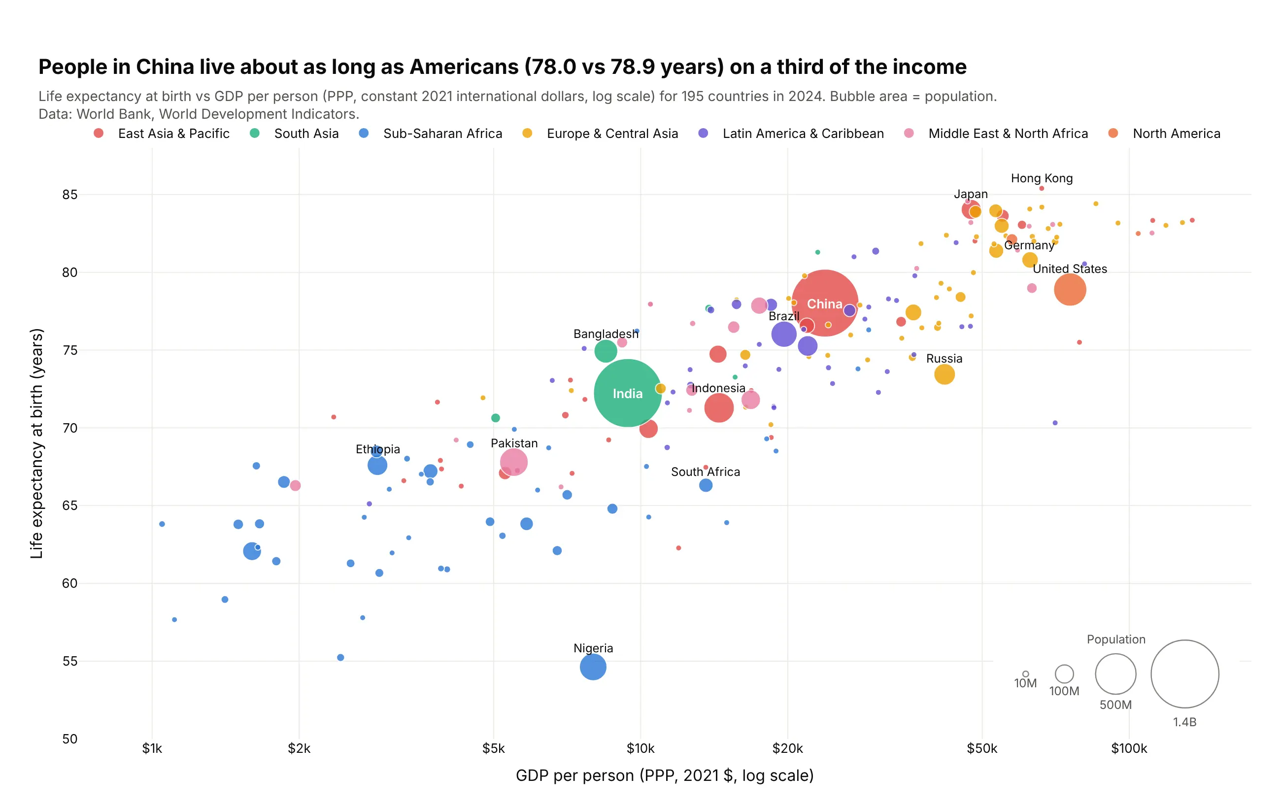
Data: World Bank, World Development Indicators, 2024.

How do you read a bubble chart? In the example above, notice these things:

• Each bubble is one country, placed left to right by its GDP per person and bottom to top by its life expectancy, so the cloud rising toward the top right shows that richer countries tend to live longer.
• A bubble's area is the country's population, which is why India and China dominate the middle of the chart while more than half of the countries are small dots, and the size legend in the bottom right gives the scale.
• The income axis is on a log scale, so each step along it multiplies income instead of adding to it, and the poorest countries on the left are spread out enough to read instead of piled against the axis.
• Color shows the region, so the blue Sub-Saharan African countries stand out as a group in the lower left, with Nigeria the lowest bubble in the chart.
• China and the United States sit at almost the same height, but the US bubble is far to the right with about three times the income per person, and the log axis makes that gap look smaller than it is.

It's often used for charts like these:

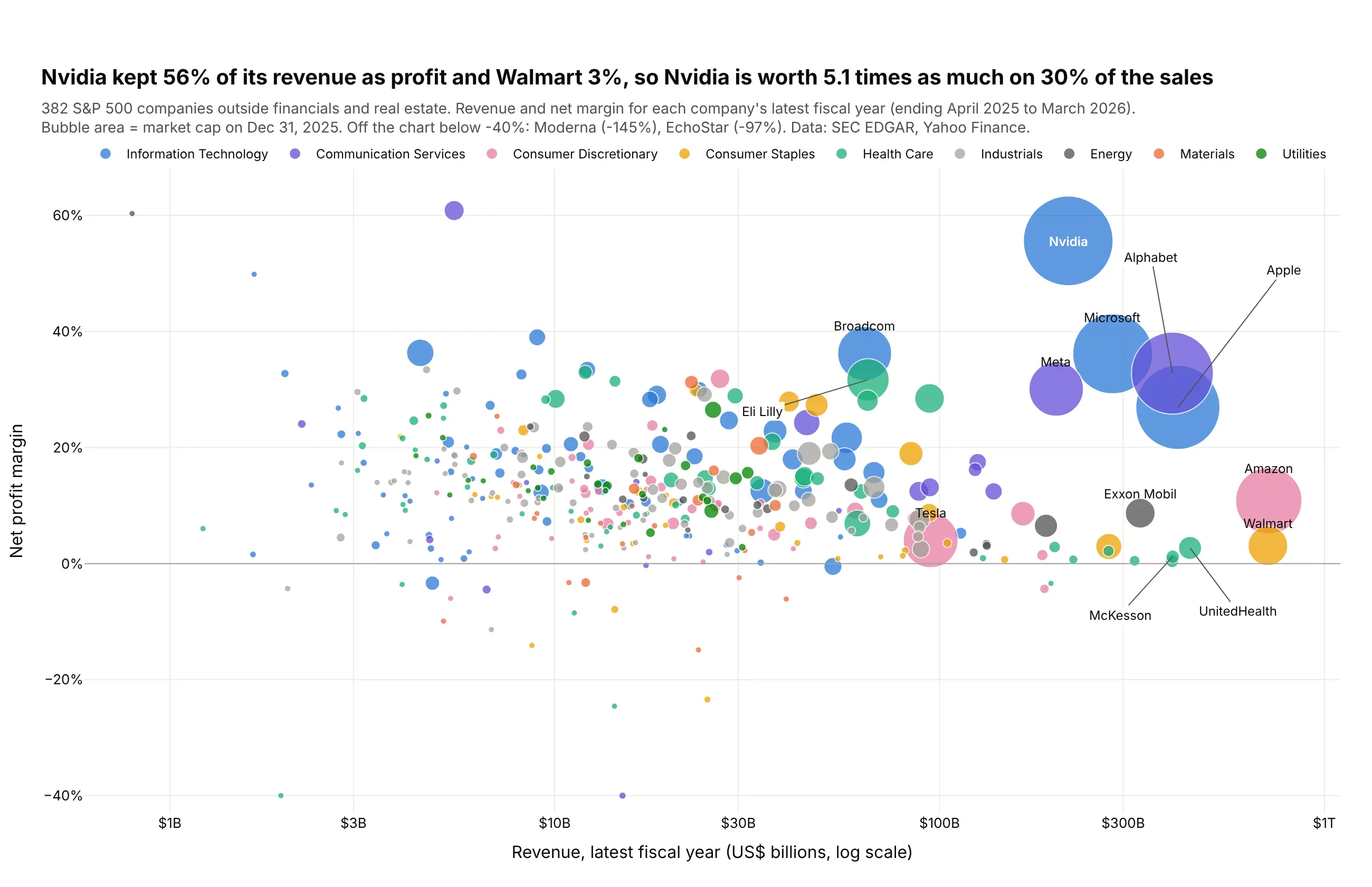
Companies by size, profitability and value. Nvidia kept 56% of its $216 billion of revenue as profit and Walmart 3% of $713 billion, so Nvidia was worth 5.1 times as much at the end of 2025. Data: SEC EDGAR, Yahoo Finance.

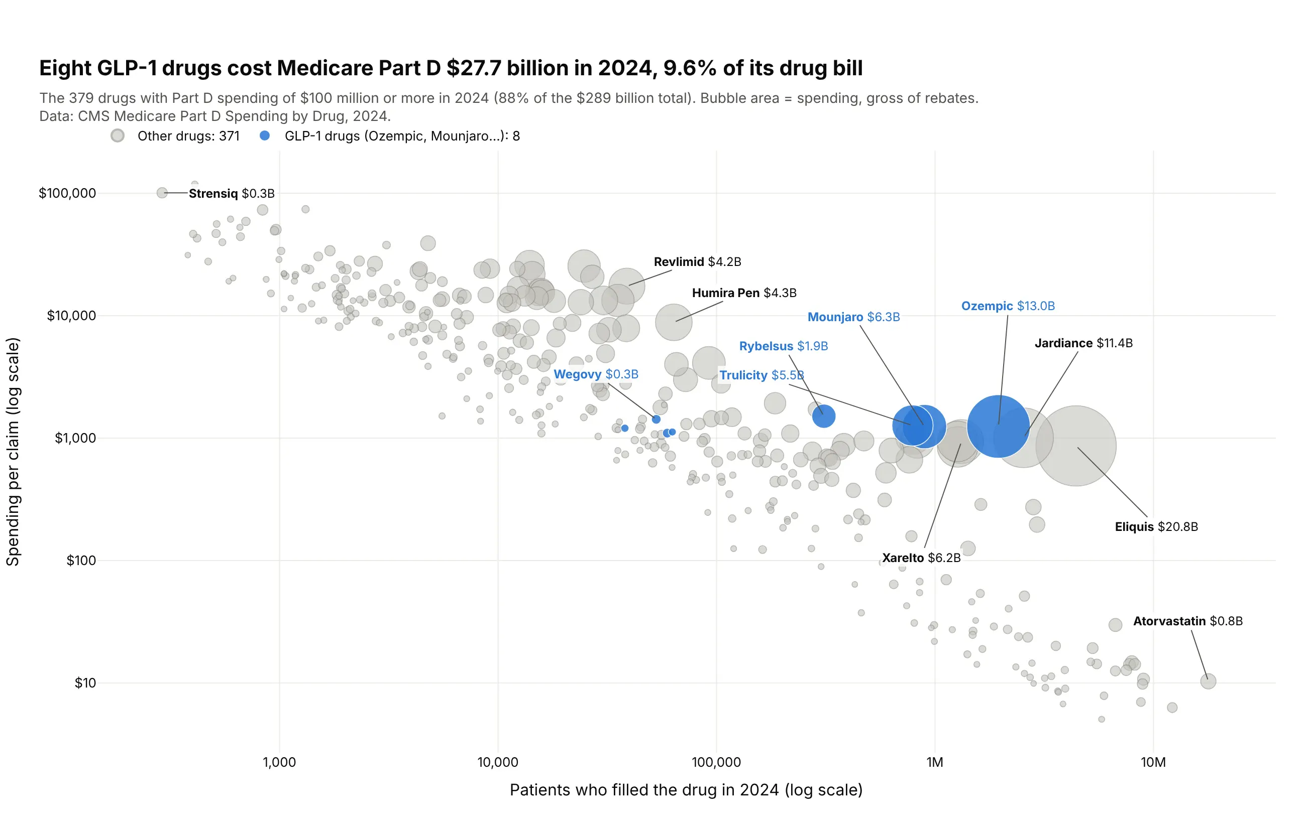
Drugs by patients, price and total spending. Eight GLP-1 drugs cost Medicare Part D $27.7 billion in 2024, 9.6% of its $289 billion drug bill, and they sit together at $1,100 to $1,500 per claim. Data: CMS Medicare Part D Spending by Drug, 2024 (before rebates).

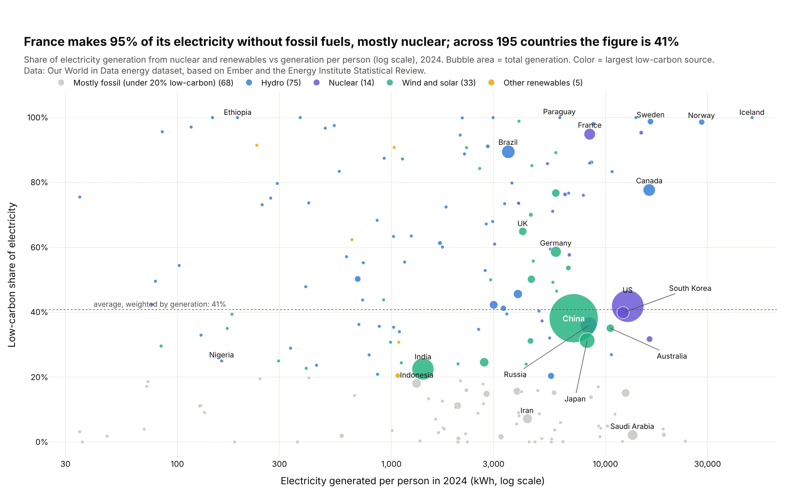
Countries by how they make electricity. France makes 95% of its electricity without fossil fuels, mostly from nuclear, while the generation-weighted figure across 195 countries is 41%. Data: Our World in Data, from Ember and the Energy Institute.

A short history

Circles sized by quantity started on maps as proportional symbols, and in 1971 the cartographer James Flannery found that readers underestimate the larger of two circles (Flannery 1971, doi:10.3138/J647-1776-745H-3667). The bubble chart became famous in 2006, when Hans Rosling showed his animated Gapminder chart of income and life expectancy in the TED talk The best stats you've ever seen. Here is that idea redrawn with Plotly on World Bank data for 2006 (not Gapminder's own data):

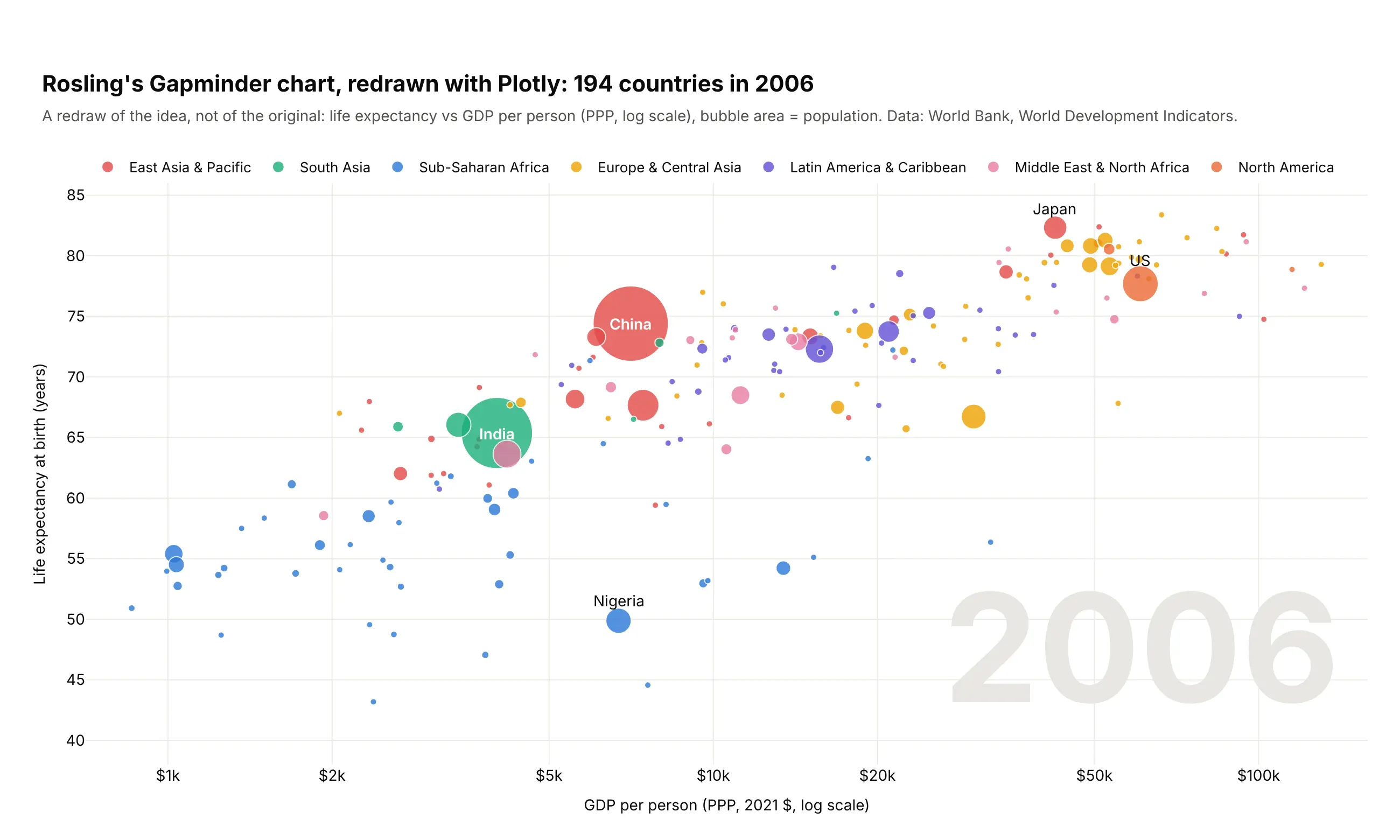
Google bought Rosling's software, Trendalyzer, in 2007, and "motion charts" spread from there. Example 1 below is a static version of the same chart for 1990, 2007 and 2024.

Alternatives to a bubble chart

Here's the same table of the 15 most populous countries drawn six ways. Some are better for the question, some worse, some just different:

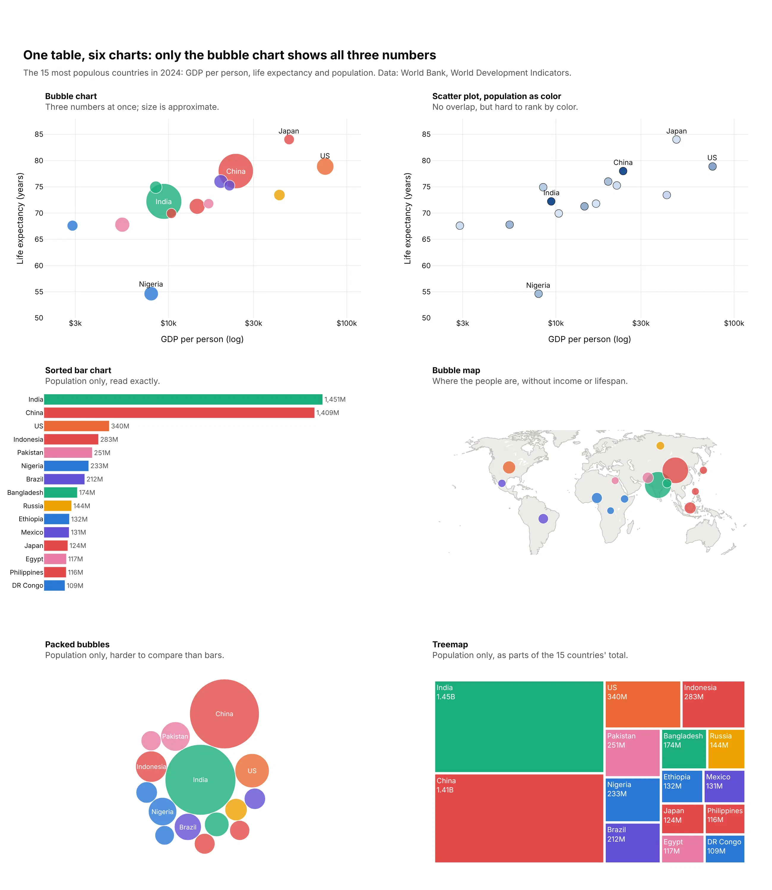
• Scatter plot with population as color (worse for size, better for overlap). Every point is the same size, so nothing hides anything else, but people can't rank countries by shade. Use it when the items are similar in size or there are too many to size.
• Sorted bar chart (better for precise comparisons). People judge length on a shared baseline more accurately than area, as Cleveland and McGill (1984) measured, so use bars when one number matters most. You lose the other two numbers.
• Bubble map (different). The same bubbles at each country's location, which answers where instead of how two numbers relate. Example 6 below is one.
• Packed bubbles (worse). Circles packed together without axes show only size, and less precisely than the bar chart next to it. We drew these with Plotly as circle shapes, after placing them with a short packing function.
• Treemap (works too, for sizes only). Shows parts of a whole and fits hundreds of items. See our treemap guide.

How to make a bubble chart

With AI

ChatGPT, Claude Code, GitHub Copilot, Cursor and other AI tools are excellent at writing Plotly code. Name Plotly in the prompt, say what x, y, size and color mean, and list the checks you want:

With Plotly Studio

Plotly Studio is a desktop app where you point an AI at a dataset and it builds charts and a Dash app around your questions. Ask for a bubble chart the same way:

Show a bubble chart of countries with GDP per person on a log x axis, life expectancy on y, bubble area by population and color by region. Label the ten most populous countries, add a size legend, and add a year slider from 1990 to 2024.

Make a bubble chart in Python or JavaScript

This is the code AI tools write under the hood. In Python, Plotly Express sizes bubbles by area and sets the scale from size_max, the diameter in pixels of the largest bubble:

With go.Scatter, set the sizing yourself, because its default sizemode is diameter:

This helper adds a size legend to a Plotly bubble chart as reference bubbles on an inset axis whose x range is in pixels:

In JavaScript, plotly.js takes the same marker options on a scatter trace:

Share it

Every Plotly chart has a Share chart button (the cloud icon in its toolbar) that uploads it to Plotly Cloud and gives you a link. Only you can see it until you change its visibility.

For a live app, put the chart in a Dash app and publish it with the Plotly Cloud CLI. Coding agents can run these commands for you:

If your data has to stay in your own cloud or data center, publish to Dash Enterprise instead.

Dos and don'ts

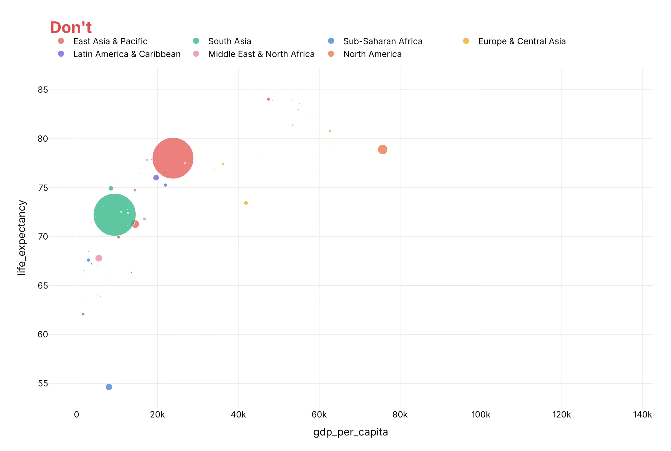
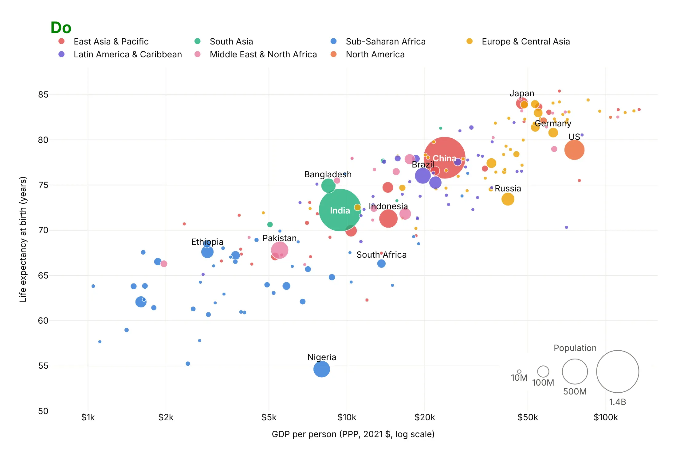
Both charts below show the same 195 countries in the same region colors. The differences are the mistakes that most often make a bubble chart misleading.

Don't size bubbles by diameter, put income on a linear axis, draw the biggest bubbles last over the small ones, or leave raw column names as axis titles. Sized by diameter, China's 6.1 times more people than Nigeria look 37 times bigger, and on the linear axis 77% of the countries pile into the left third of the chart:

Do size by area with sizemode="area", use a log axis for income, draw big bubbles first with thin white outlines, label the countries the story needs and add a size legend:

Use color for one other thing

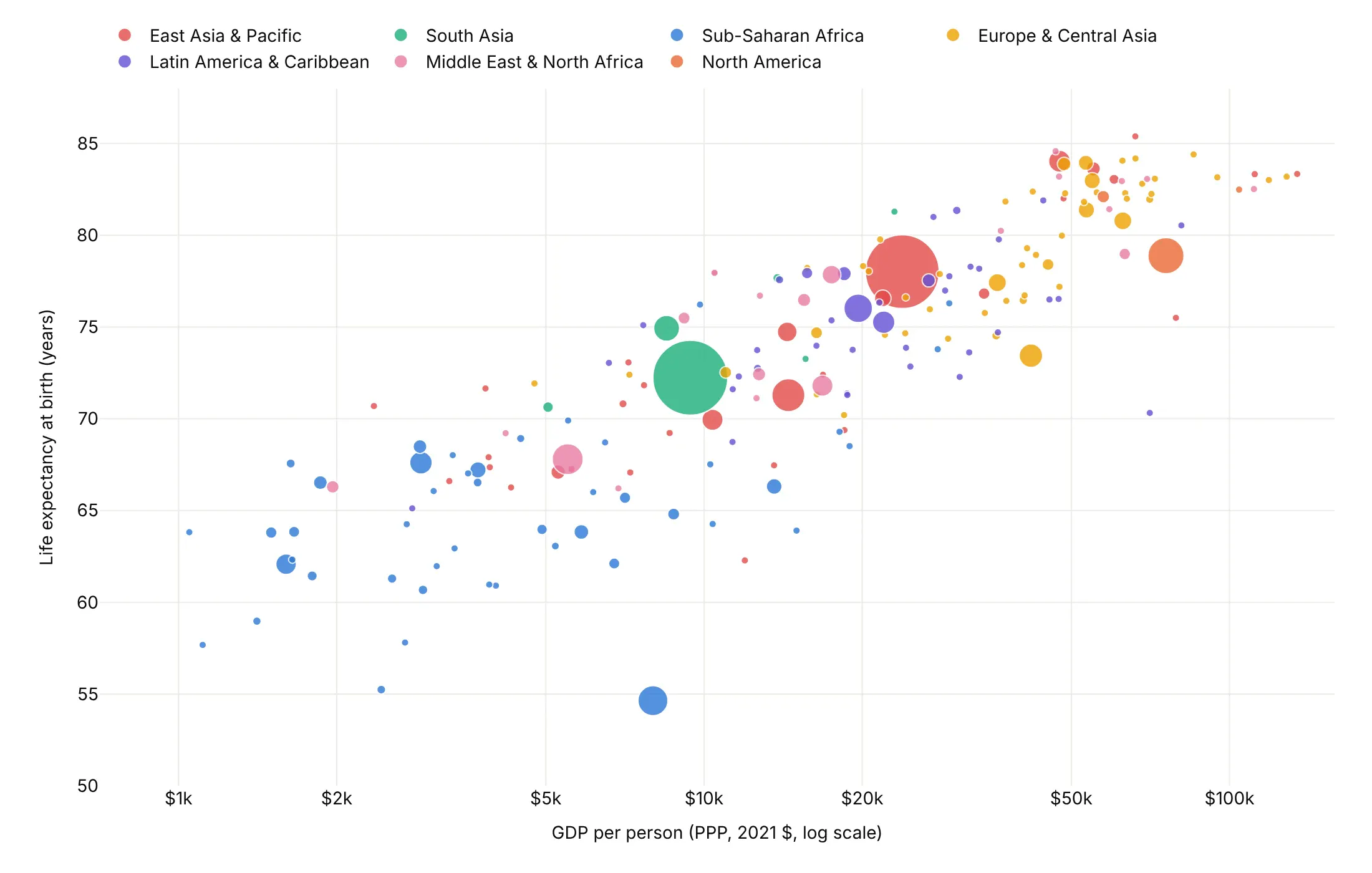
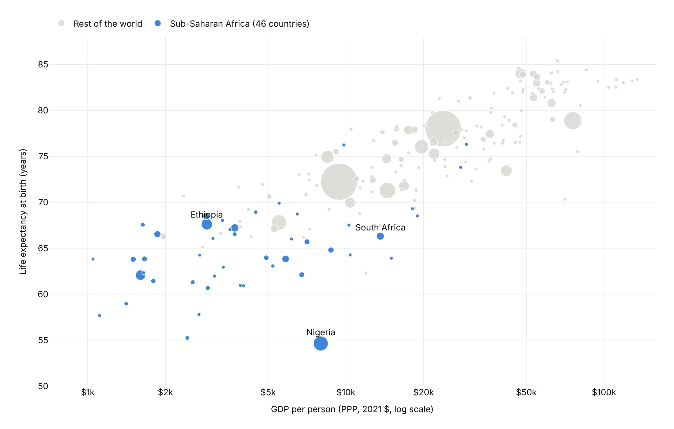
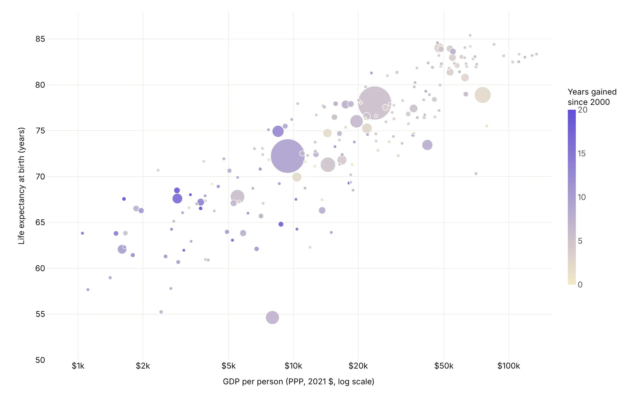
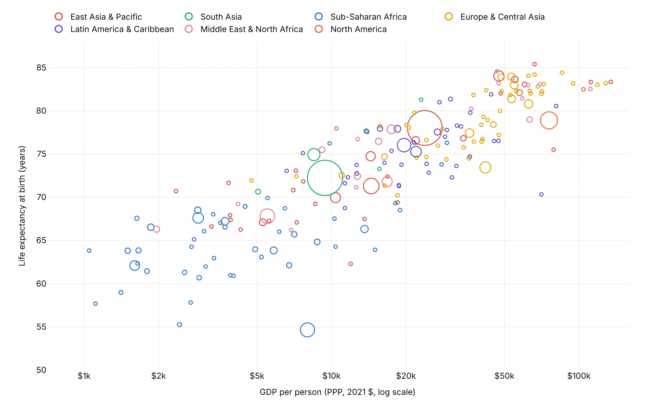
Position and area already show three numbers, so color is free for one more. Here are four options on the same data.

By category. Region is a good default, because it groups countries that sit together on the chart.

Highlight one story. Sub-Saharan Africa's 46 countries are the only color, and everything else is gray.

A fourth number. Here it's the years of life expectancy gained since 2000, for the 189 countries with data for both years, on a scale capped at 0 and 20.

Hollow bubbles. Colored outlines with no fill keep every bubble visible where they overlap.

Checklist

Do

• Size by area, with sizeref = 2 * max(size) / max_px**2 and a largest bubble of 40 to 90 pixels.
• Draw big bubbles first, with a thin white outline and 0.6 to 0.85 opacity.
• Use a log axis when a variable spans more than about 20 times.
• Add a size legend and label the bubbles the story needs.
• Write the takeaway in the title and say what size and color mean in the subtitle.

Don't

• Size by diameter, because a value 6 times bigger then looks 36 times bigger.
• Size by rates or averages, because area reads as a total.
• Rely on an animation in a static report; use small multiples or connected bubbles.
• Let bubbles at the edge get cut off; widen the axis range or set cliponaxis=False.

Options to customize

These are the go.Scatter (and px.scatter) options that matter most for bubble charts. The full list is in the Plotly bubble chart documentation.

1. size, size_max (px only): the column for bubble size, and the diameter in pixels of the largest bubble (default 20; 40 to 90 is usually better).
2. marker.size: the bubble size, one value per point.
3. marker.sizemode: "diameter" (the default) or "area". Use "area" for quantities.
4. marker.sizeref: the scale. In area mode the diameter is sqrt(value / sizeref), so set it to 2 * max(size) / max_px**2.
5. marker.sizemin: a minimum diameter in pixels, so tiny values stay visible (2 to 4 px).
6. marker.opacity, marker.line: transparency and outline, 0.55 to 0.85 with a white line when bubbles overlap.
7. marker.color, colorscale, cmin, cmax, colorbar: a category or a fourth number as color.
8. mode="markers+text", textposition: labels on the bubbles; a list sets one position per point, for up to about 50 bubbles.
9. layout.annotations (showarrow, ax, ay): labels on leader lines for crowded clusters. On a log axis, pass log10(x).
10. xaxis.type="log": a log axis for skewed variables such as income or revenue.
11. legend.itemsizing="constant": keeps legend markers one size instead of copying a random bubble.
12. animation_frame, animation_group (px only): frames and identity for a Gapminder-style animation.
13. facet_col, facet_row (px only): small multiples that share one size scale.
14. go.Scattergl: the WebGL renderer, with the same marker options, for more than about 10,000 bubbles.
15. go.Scattergeo, go.Scattermap: bubbles on a map.
16. cliponaxis: set to False to draw bubbles past the edge of the plot area.

More bubble chart examples

Ten more bubble charts built from real public data, each with its source, the technique that makes it work and a prompt to rebuild it.

1. Thirty-four years of health and wealth, as small multiples

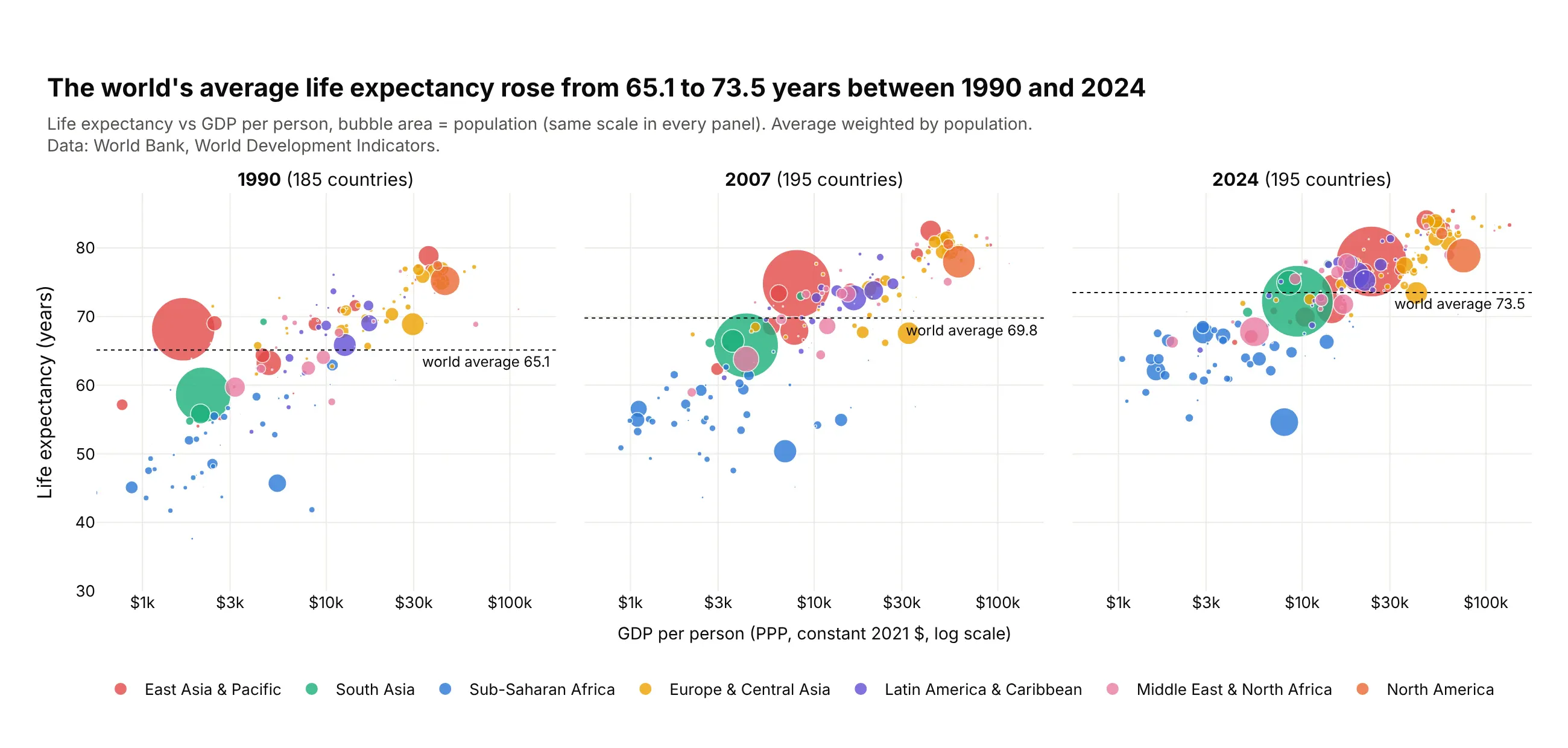
On a page, the Gapminder animation becomes three frames side by side. The population-weighted world average rose from 65.1 years in 1990 to 73.5 in 2024, and China and India moved up and to the right. Data: World Bank, World Development Indicators.

Tip: px.scatter(facet_col="year") uses one size scale for every panel, so a bubble's size means the same thing in each year.

2. What gets reported for eight big drugs

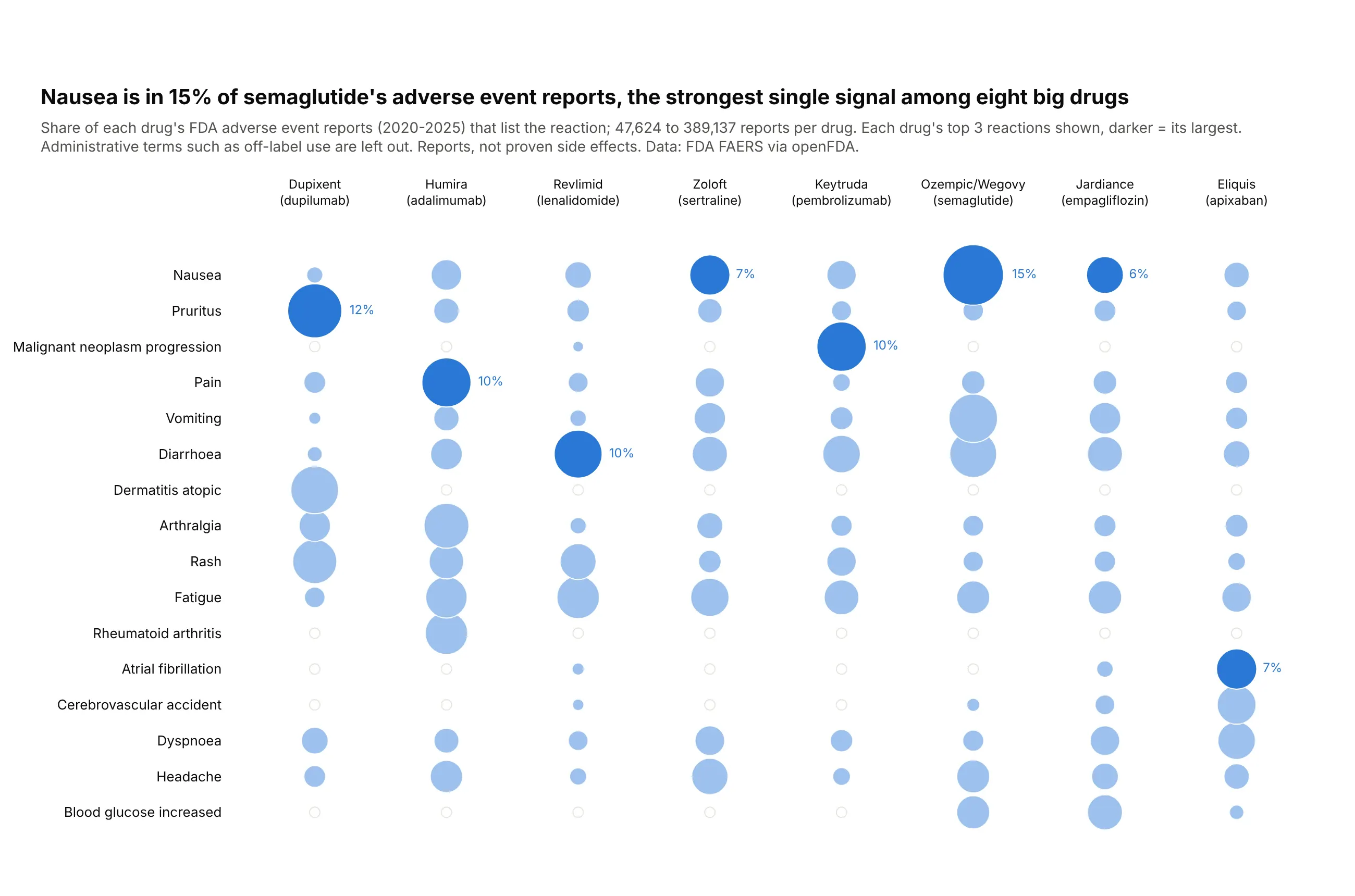
With categories on both axes, a bubble chart becomes a matrix. Nausea is in 15.1% of semaglutide's 58,221 reports, the largest share in the grid, and each drug has its own signature. Reports are not proven side effects. Data: FDA FAERS via openFDA, 2020-2025.

Tip: a light gray ring behind every cell, so an empty cell reads as "close to zero" instead of missing.

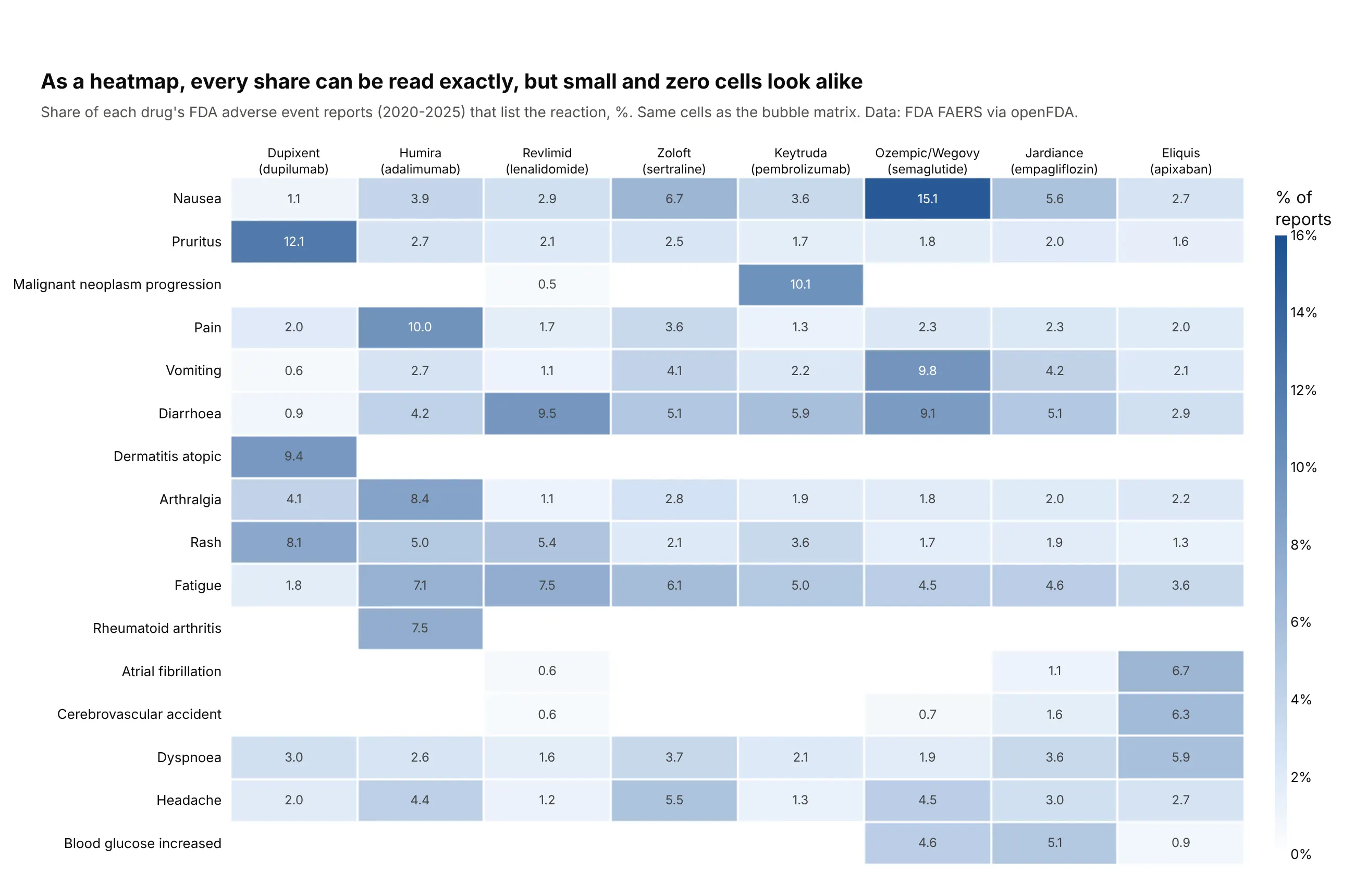
Another way to see it: a heatmap of the same cells prints every share, but cells under 1% and missing cells look alike.

3. Government debt and deficits

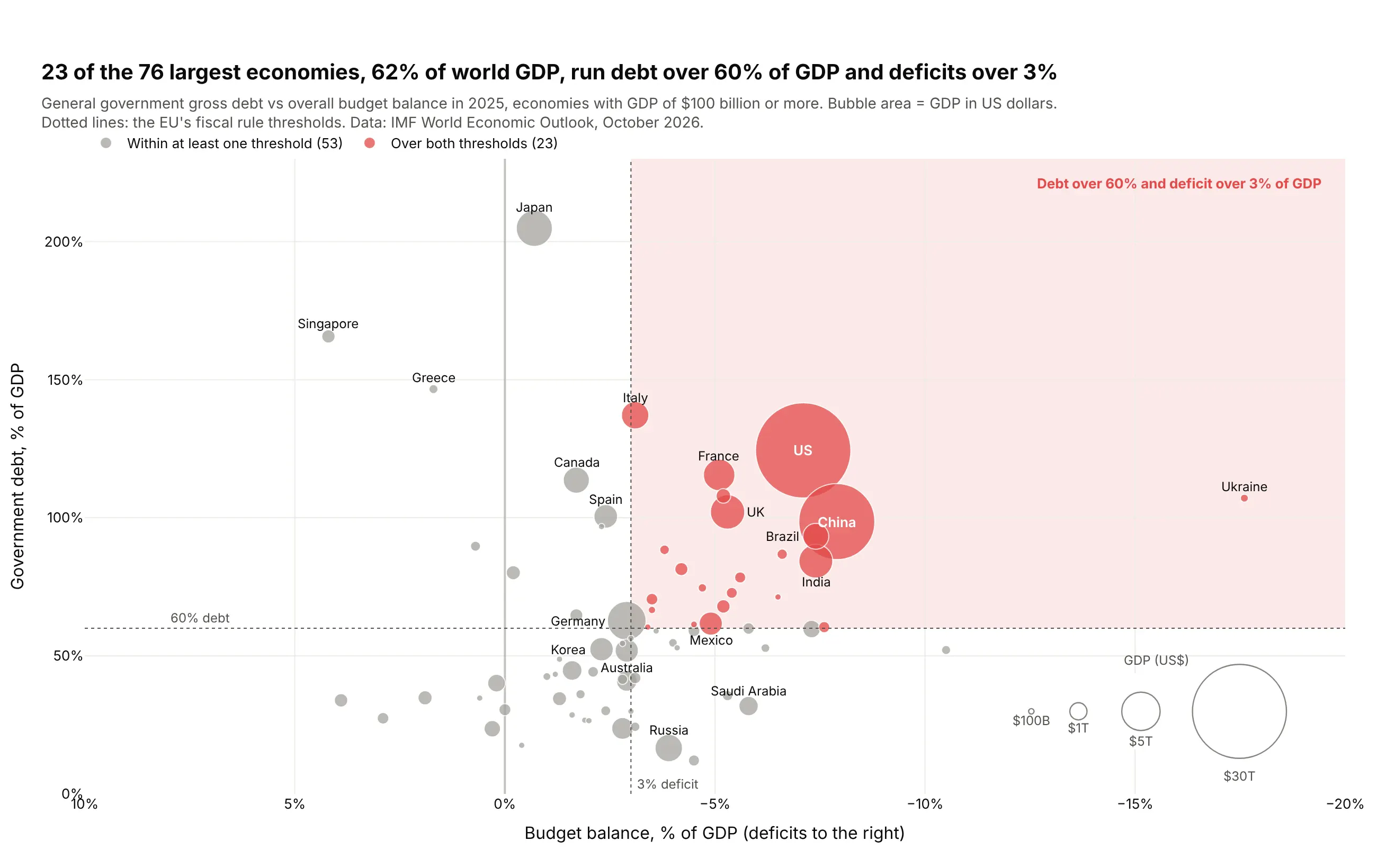
Twenty-three of the 76 largest economies, 62% of world GDP, have debt over 60% of GDP and a deficit over 3%, the EU's two fiscal thresholds. Japan's debt is the highest of the 76 at 205% of GDP, with a deficit of 0.7%. Data: IMF World Economic Outlook, October 2026.

Tip: reference lines and a shaded quadrant with add_vline, add_hline and add_shape(type="rect", layer="below") turn the chart into a rule check.

4. US metros: people moved, prices rose everywhere

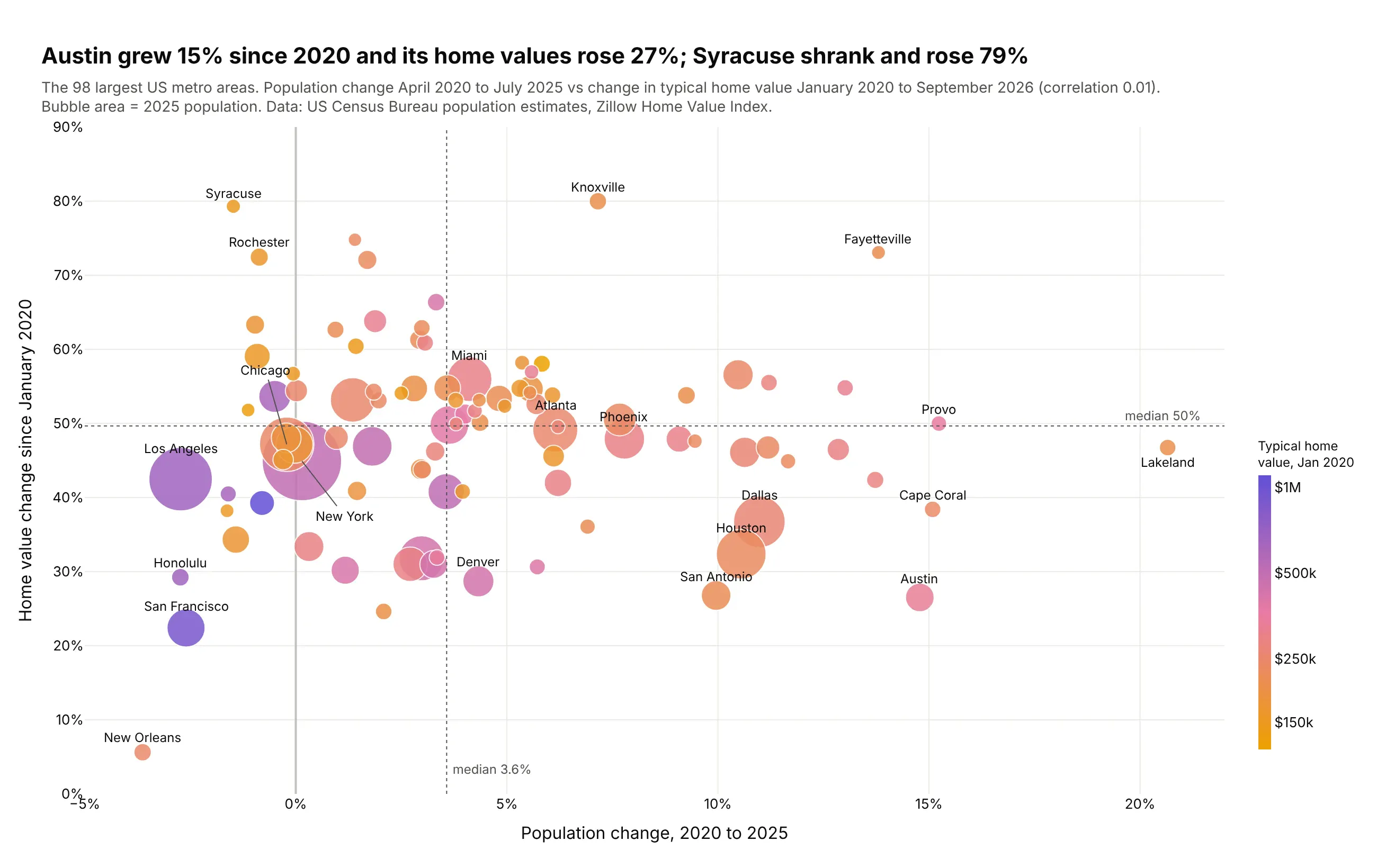
Population growth didn't predict price growth: the correlation across the 98 largest metros is 0.01. Austin grew 15% and its home values rose 27%, while Syracuse lost people and rose 79%. Data: US Census Bureau population estimates, Zillow Home Value Index.

Tip: a continuous colorscale on the log of the 2020 price adds a fourth variable, and shows that cheaper metros rose more.

5. How hard US power plants ran in 2025

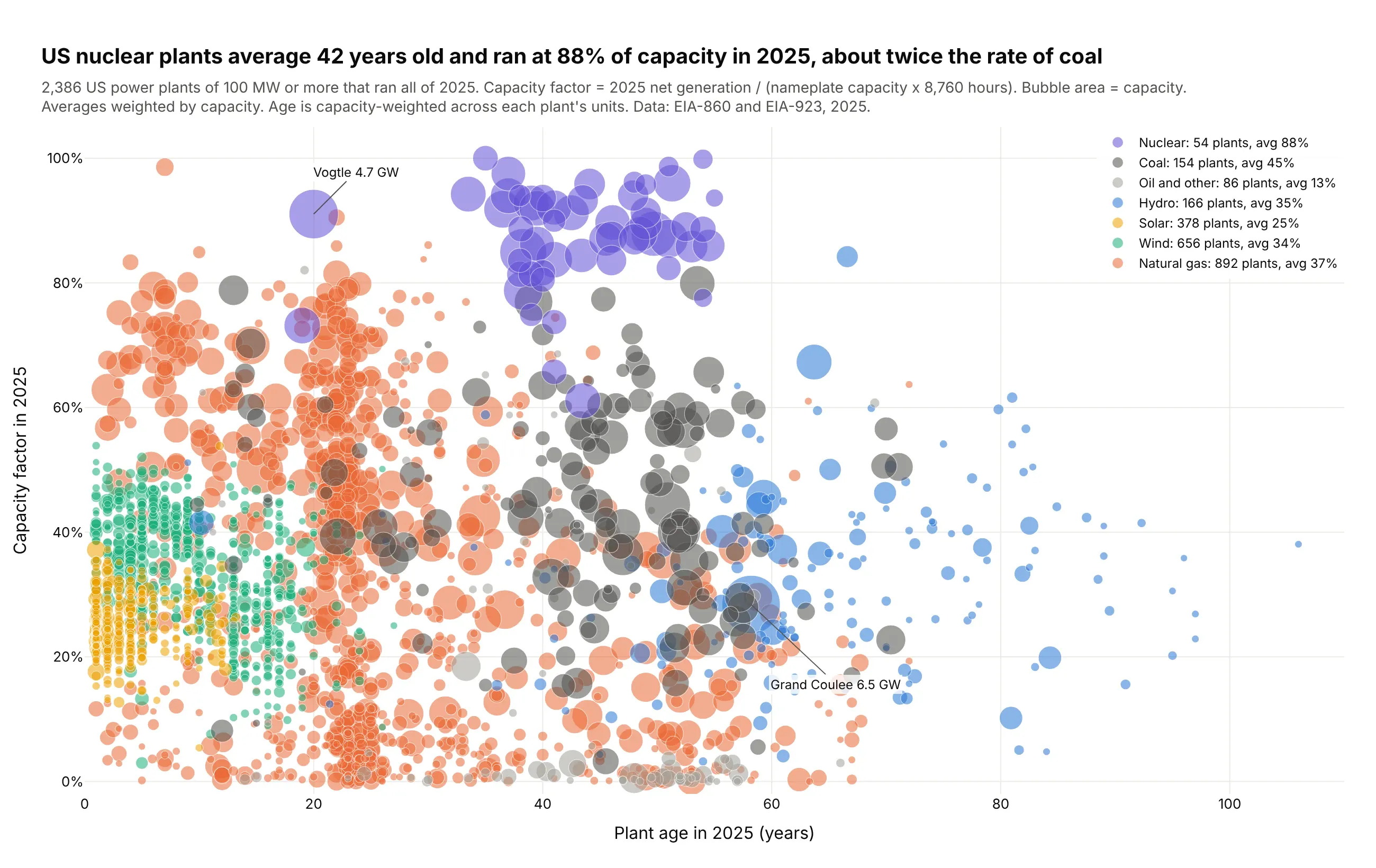
US nuclear plants are 42 years old on average and ran at 88% of capacity in 2025, about twice the rate of coal (45%). Gas plants spread from almost idle peakers to baseload. Data: EIA-860 and EIA-923, 2025.

Tip: with 2,386 overlapping bubbles, 0.55 opacity, a thin white outline and drawing the most numerous fuel first keep every cloud visible.

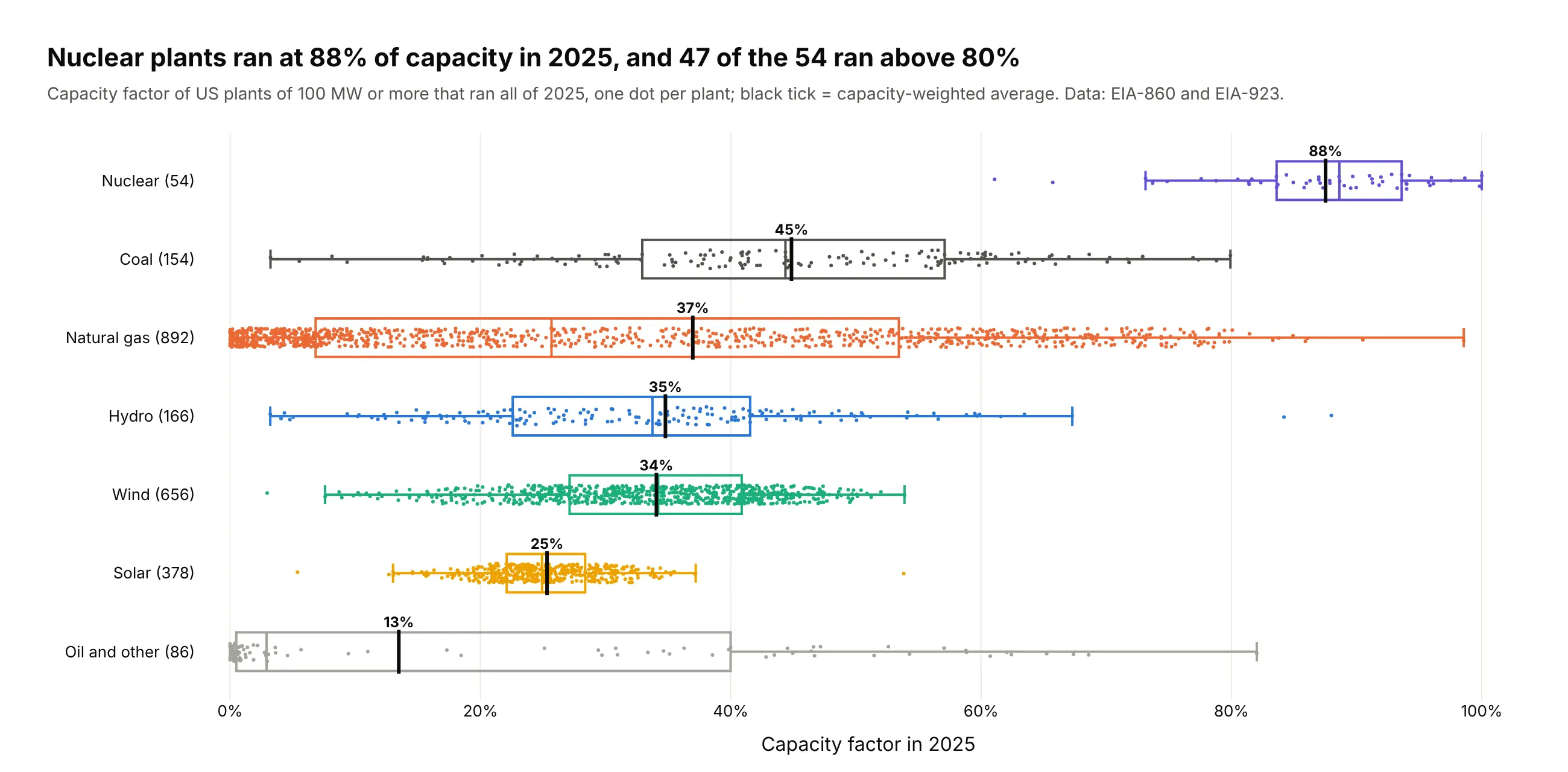
Another way to see it: box plots with every plant as a dot show each fuel's spread directly: 47 of the 54 nuclear plants ran above 80%.

6. Every US power plant on a map

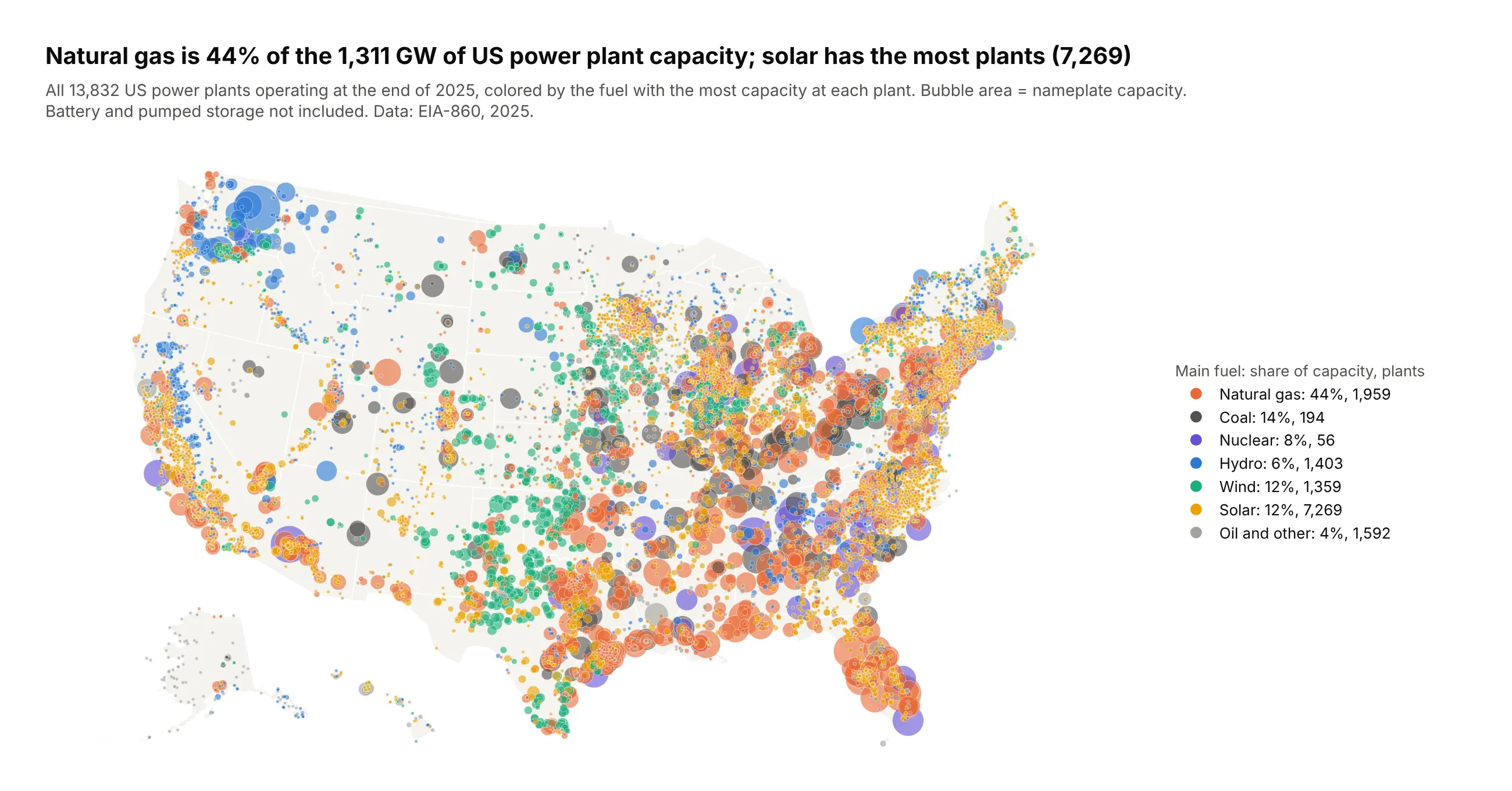
Natural gas is 44% of the 1,311 GW of US plant capacity, but solar has the most plants (7,269), mostly small. The map shows the geography the numbers hide: wind on the Plains, hydro on the Columbia River. Data: EIA-860, 2025.

Tip: one go.Scattergeo trace sorted big to small, plus empty traces (lon=[None]) per fuel for the legend.

7. The paths of the biggest emitters

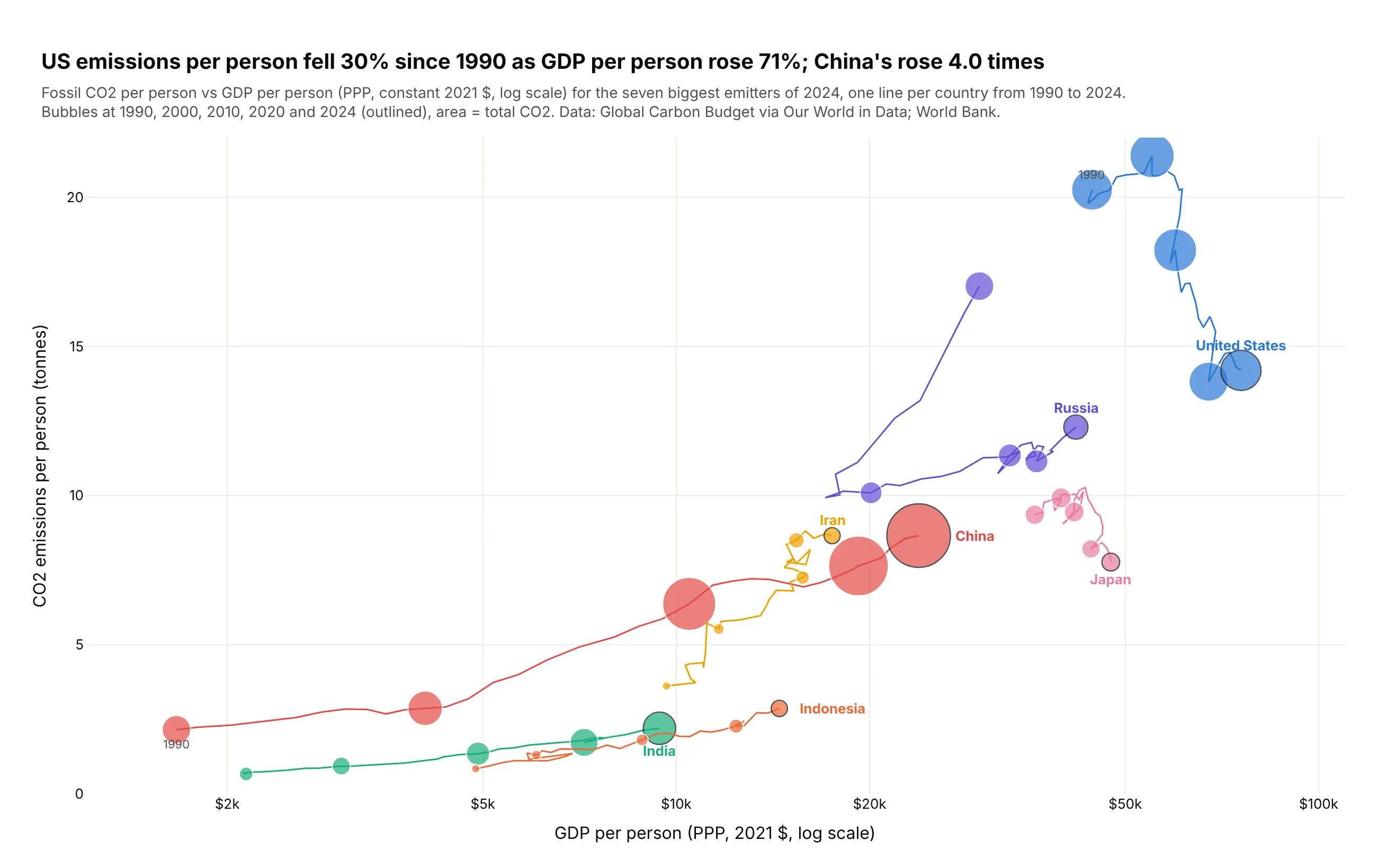
US emissions per person fell 30% since 1990 as GDP per person rose 71%, while China's rose 4.0 times. A connected bubble chart shows a whole path at once, which an animation can only show one frame at a time. Data: Global Carbon Budget via Our World in Data; World Bank.

Tip: a thin line through every year, bubbles only every ten years, and the country name at the end of the path instead of a legend.

8. Every magnitude 6+ earthquake since 2000

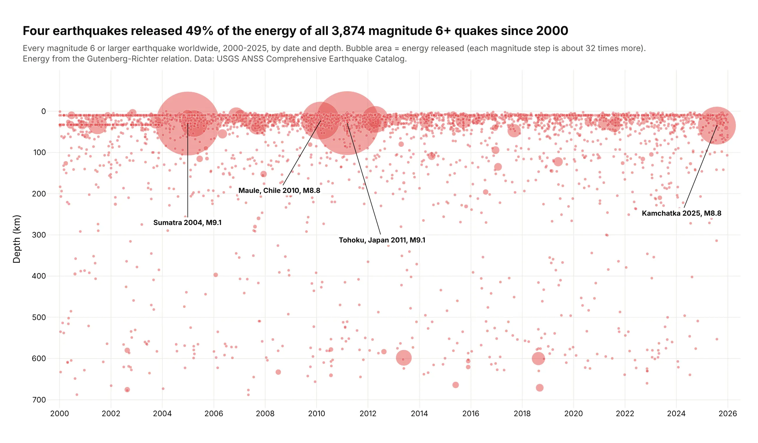
Sized by energy instead of magnitude, four earthquakes released 49% of the energy of all 3,874 since 2000. Each magnitude step is about 32 times more energy, which a magnitude-sized bubble would hide. Data: USGS ANSS Comprehensive Earthquake Catalog.

Tip: size by the physical quantity (energy) rather than a log-scale index (magnitude), and set sizemin so small events still show.

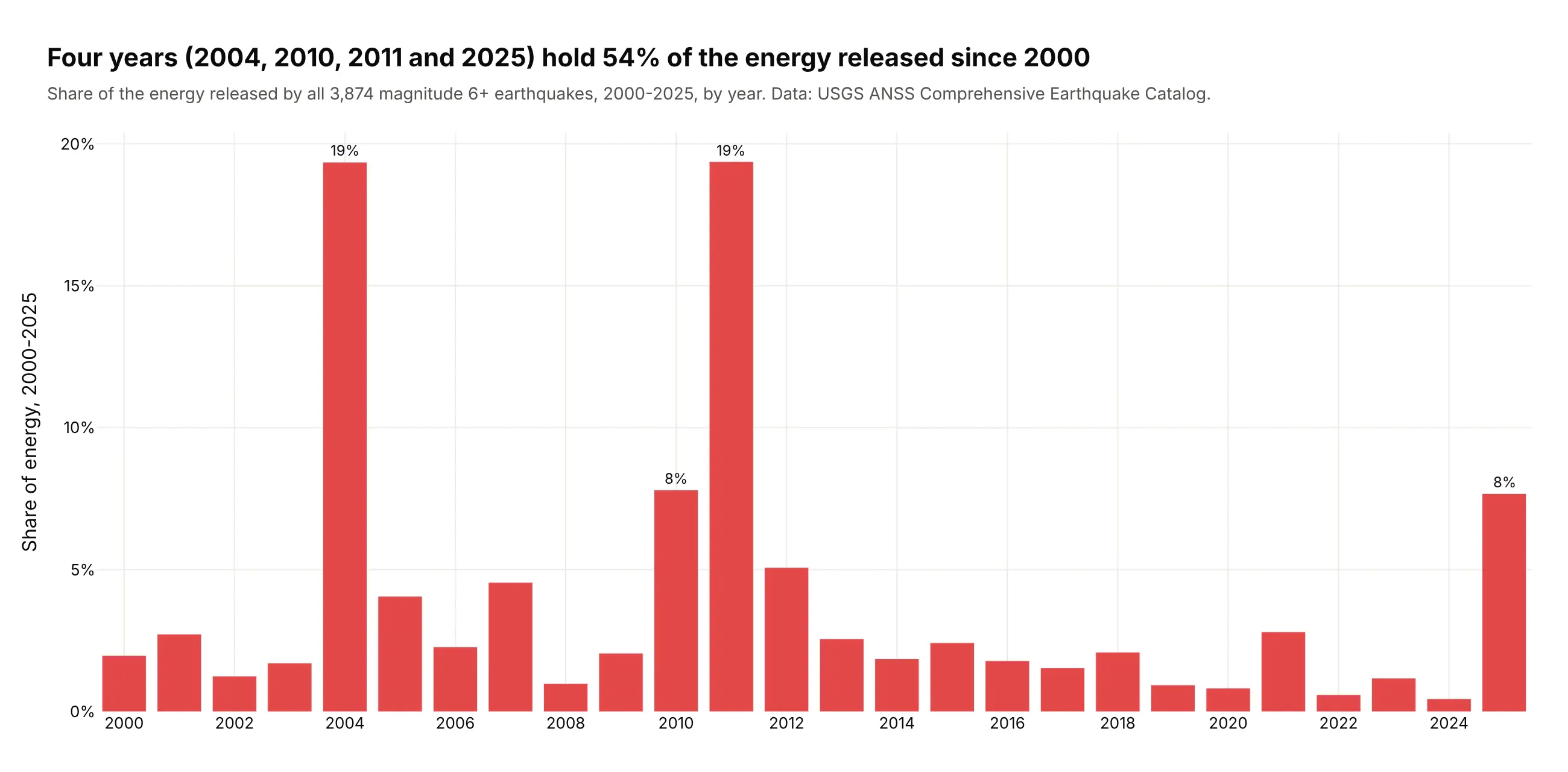
Another way to see it: a bar chart of energy by year shows that 2004, 2010, 2011 and 2025 hold 54% of the total, but loses the individual quakes and their depth.

9. NFL quarterbacks in 2025

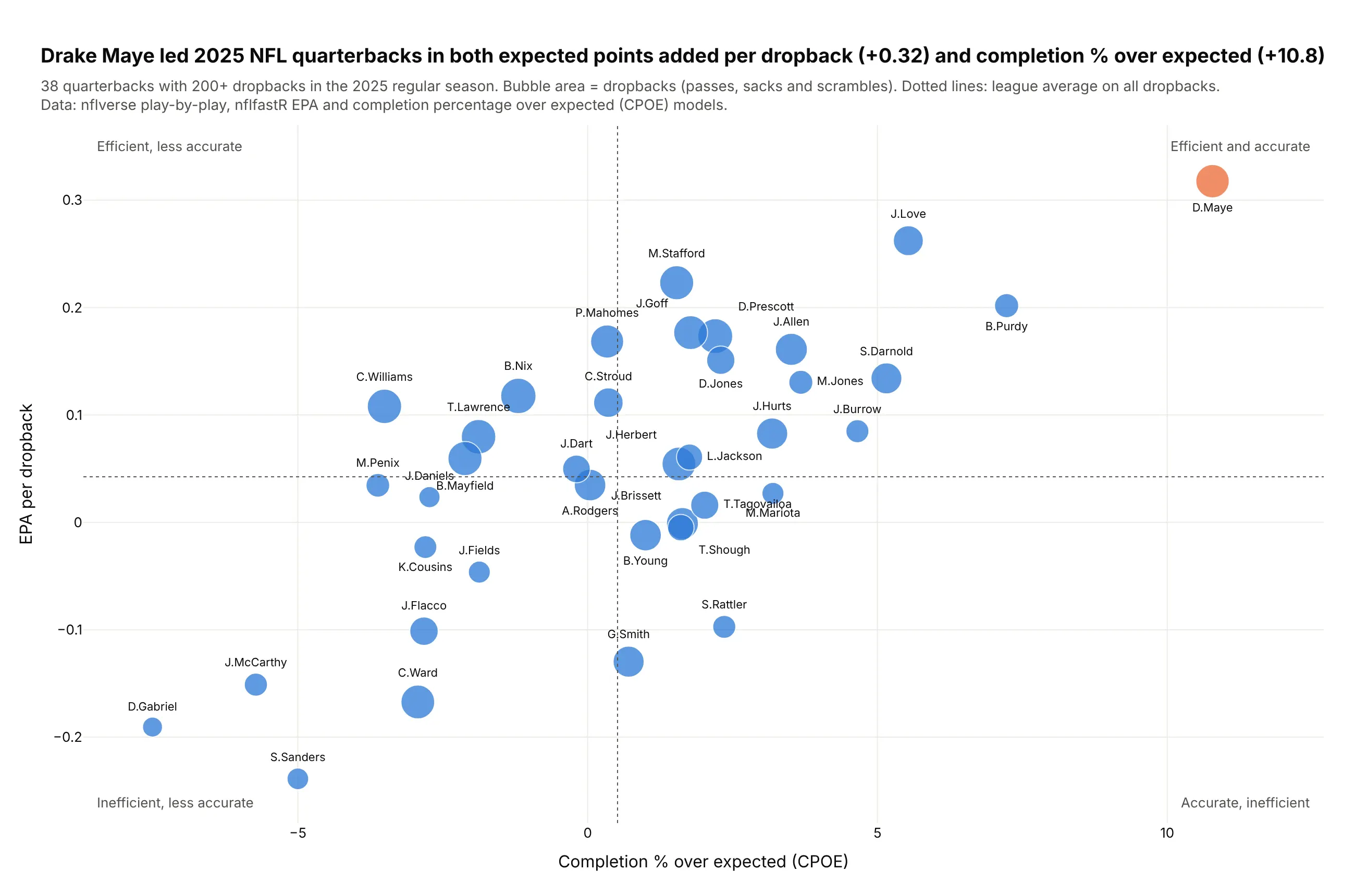
Drake Maye led the 38 starters in both expected points added per dropback (+0.32) and completion percentage over expected (+10.8). Bubble area adds the volume behind each rate. Data: nflverse play-by-play, nflfastR models, 2025 regular season.

Tip: with 38 bubbles every one can carry its name, using mode="markers+text" and a per-point textposition list to fix collisions.

10. Who runs Phase 3 trials, and how many stop early

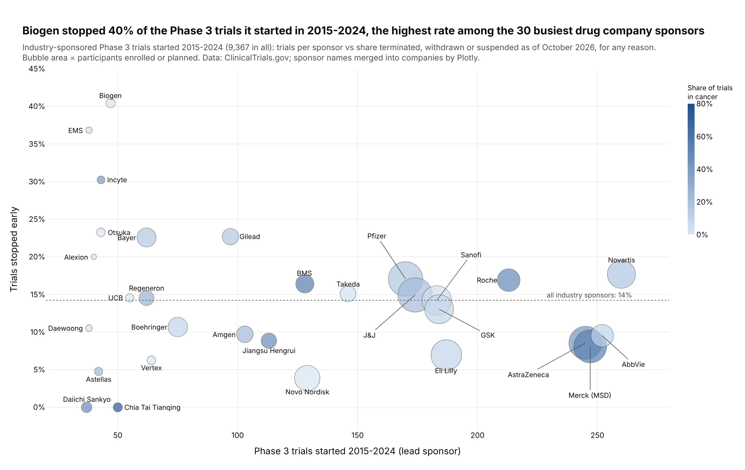
Biogen stopped 40% of the 47 Phase 3 trials it started from 2015 to 2024, the highest rate among the 30 busiest industry sponsors, against 14% for all 9,367 industry trials. Trials stop for many reasons, including business decisions. Data: ClinicalTrials.gov.

Tip: a single-hue continuous color for a share (cancer trials) adds a fourth variable without competing with the size.