Chris Parmer

October 24, 2026

Contour Plots - A Complete Guide

TL;DR

A contour plot draws lines of equal value across two dimensions: equal elevation on a topographic map, equal pressure on a weather map, equal implied volatility on an options surface.
Contour plots are also known as contour maps, contour charts and contour graphs, and are similar to heatmaps and 3D surface plots.
Use one for a smooth quantity measured on a grid, or for the density of thousands of overlapping points (earthquakes, pitches, patients).
Use a heatmap instead when the cells themselves are the data (noisy values, categorical axes), and a line chart of one slice when exact values matter.
Any coding agent can make one with Plotly. In Python it's go.Contour(x=..., y=..., z=...) for a grid and px.density_contour(df, x=..., y=...) for points.

What is a contour plot?

Contour plots look like this:

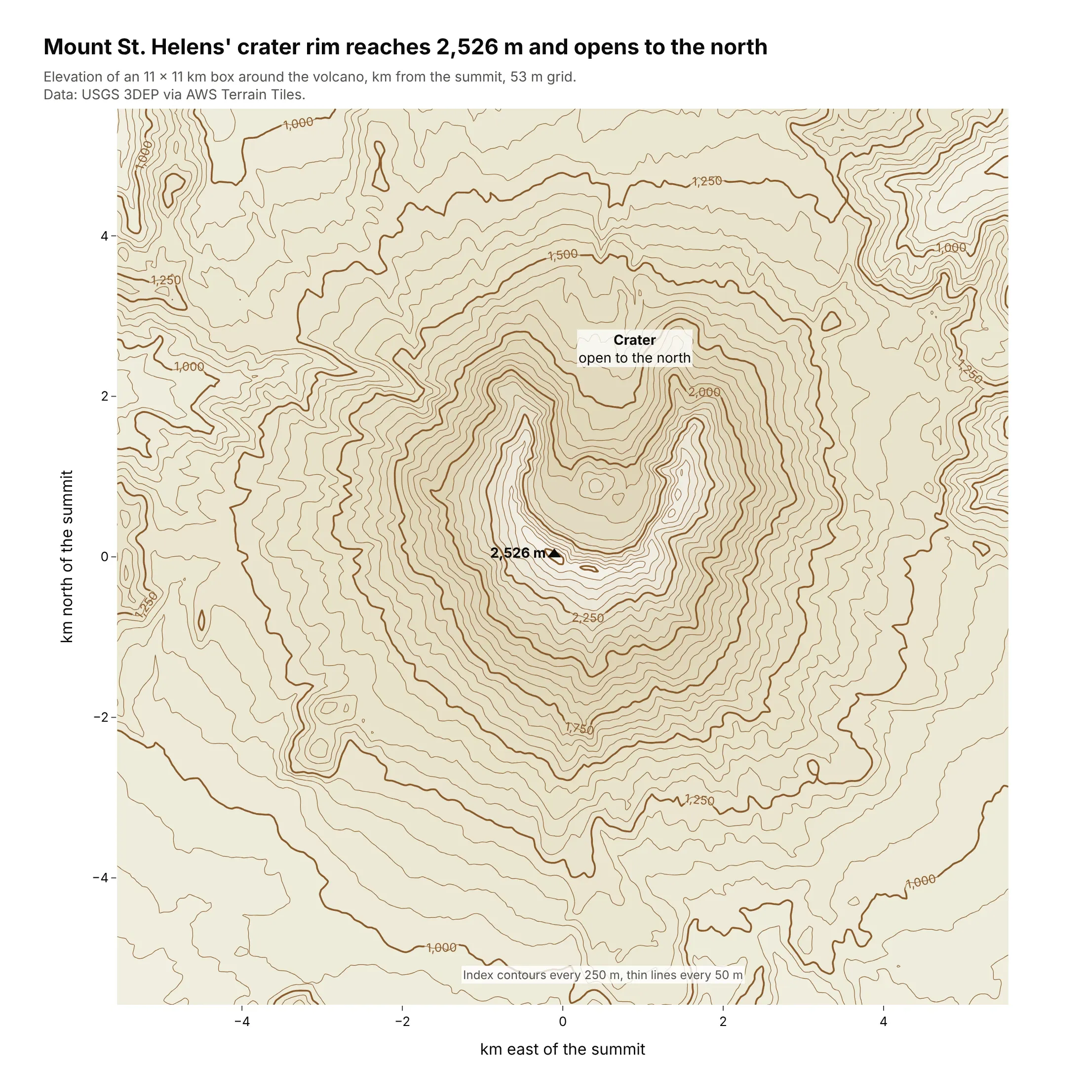
Topographic map of Mount St. Helens with thin brown contours every 50 m and bold labeled index contours every 250 m over a pale fill; the horseshoe crater opens to the north and the highest grid cell is 2,526 m

Data: USGS 3DEP elevation via the AWS Terrain Tiles open dataset.

How do you read a contour plot? In the example above, notice these things:

Each line joins points at the same elevation, so if you walked along one you would neither climb nor descend. The thin lines are 50 m apart, and every fifth one is a bold, labeled index contour.
The labels on the bold lines tell you which way is up, rising from the edges of the box toward the 2,250 m line just below the summit triangle. Without them, a ring around a hill and a ring around a hollow would look the same.
The spacing shows the slope. Where the lines bunch together, as just below the crater rim, the ground is steep, and where they spread apart, as at the southern foot of the mountain, it is gentle.
The rings around the top form a horseshoe instead of closed circles, because the crater is open to the north. Inside the horseshoe the lines step back down toward the crater floor, so the rim around the summit triangle is higher than the middle of the crater.
Watch out for the summit value. The triangle marks the highest cell of the elevation grid, 2,526 m, and averaging the grid smooths the peak, so the real summit is a little higher than the map shows.

It's often used for charts like these:

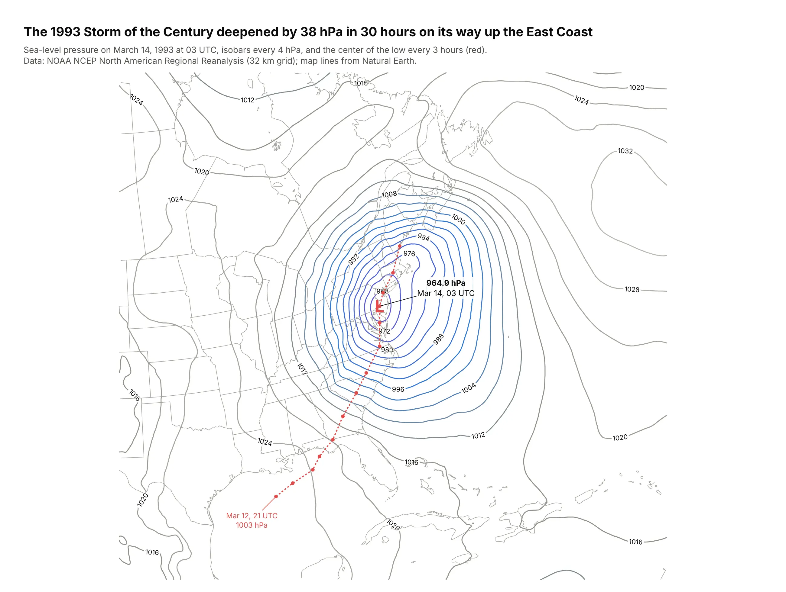
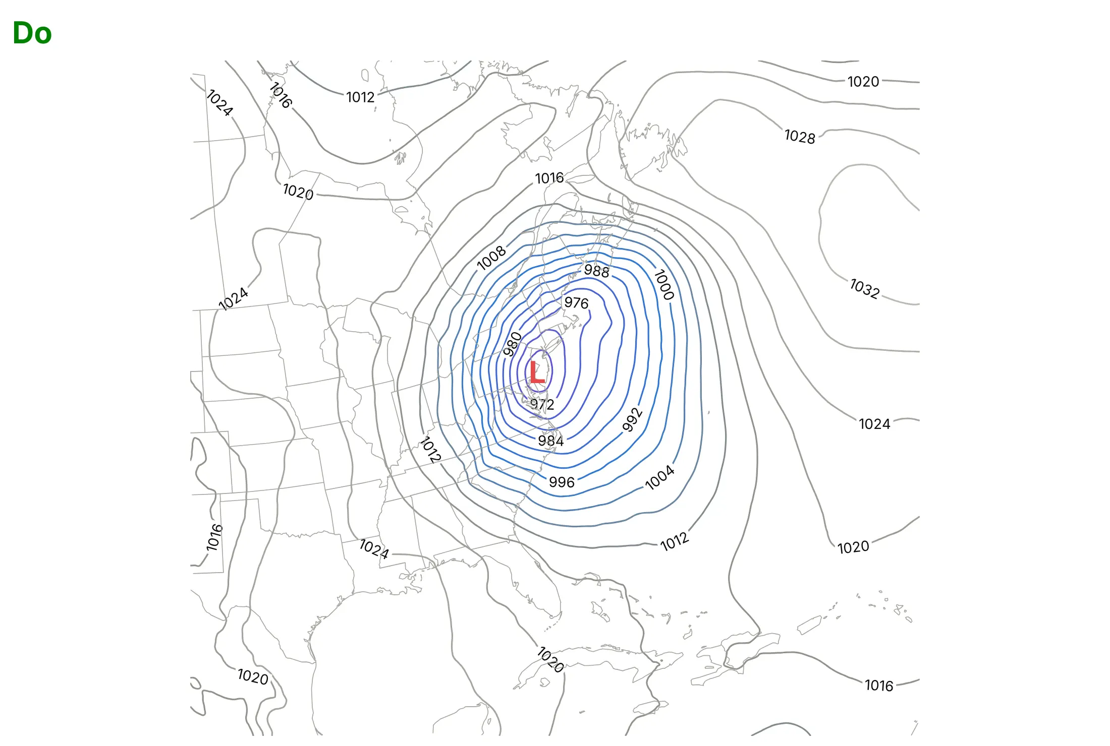
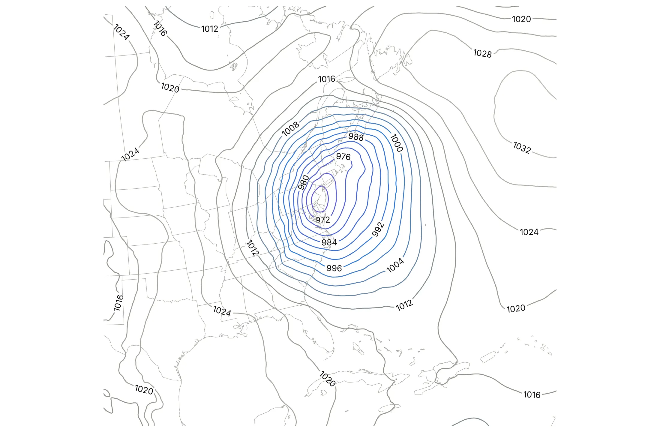
Weather map of sea-level pressure on March 14, 1993 at 03 UTC with isobars every 4 hPa over coastlines and state lines, the storm's track in red from the Gulf of Mexico, and the low of 964.9 hPa near Philadelphia

A weather map. In reanalysis data, the 1993 Storm of the Century deepened by 38 hPa in 30 hours, from 1003.0 hPa over the Gulf of Mexico to 964.9 hPa near Philadelphia, and the tight rings of isobars show where the wind was strongest. Data: NOAA NCEP North American Regional Reanalysis; Natural Earth map lines.

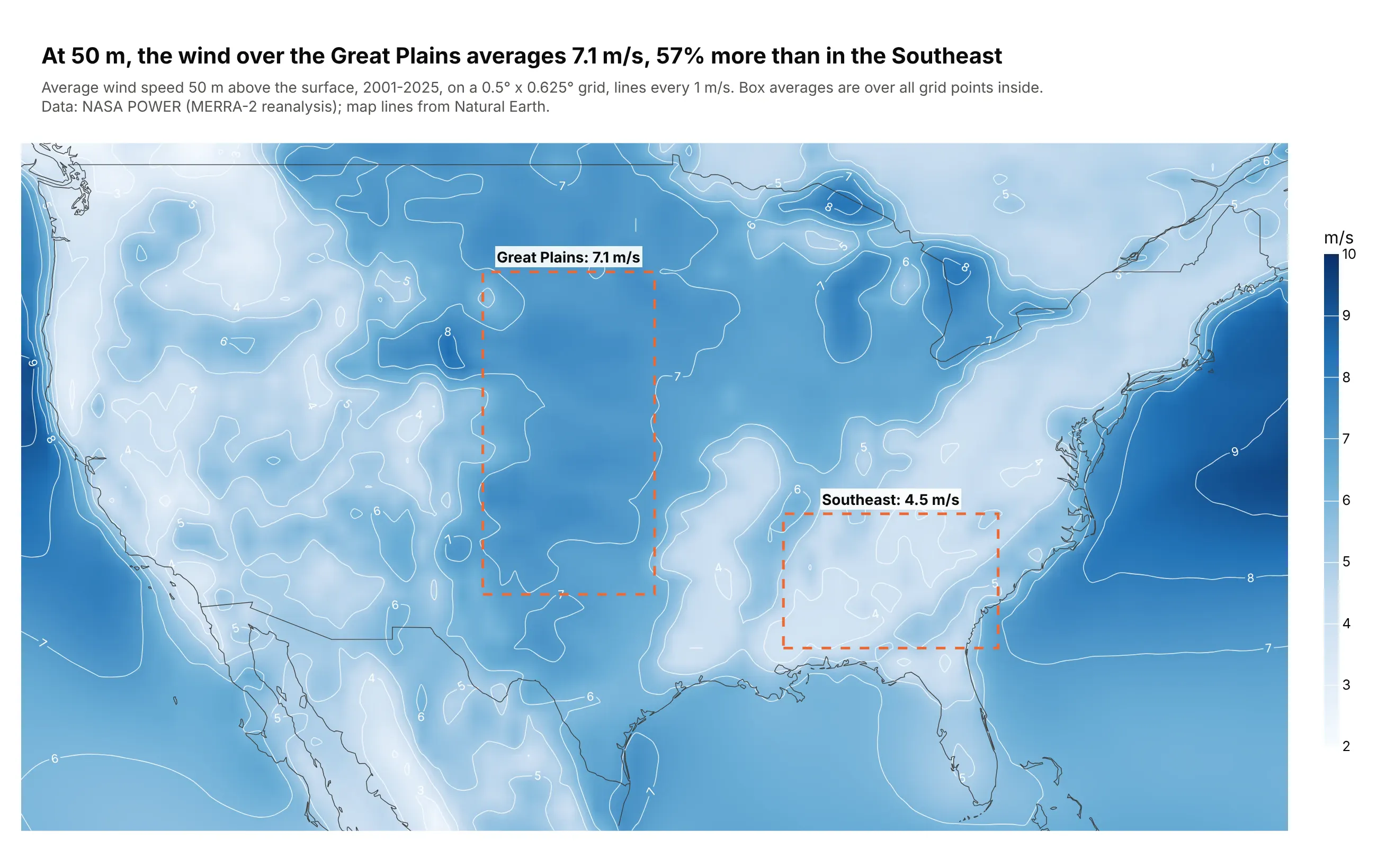
Map of average wind speed at 50 m over the contiguous US, 2001-2025, smooth blue shading with labeled lines every 1 m/s, a dashed box over the Great Plains at 7.1 m/s and another over the Southeast at 4.5 m/s

A resource map for energy planning. At 50 m, the wind over the Great Plains averages 7.1 m/s, 57% more than the Southeast's 4.5 m/s, and the strongest resource on the map is offshore, up to 9.5 m/s east of the Mid-Atlantic. Data: NASA POWER climatology (MERRA-2 reanalysis), 2001-2025.

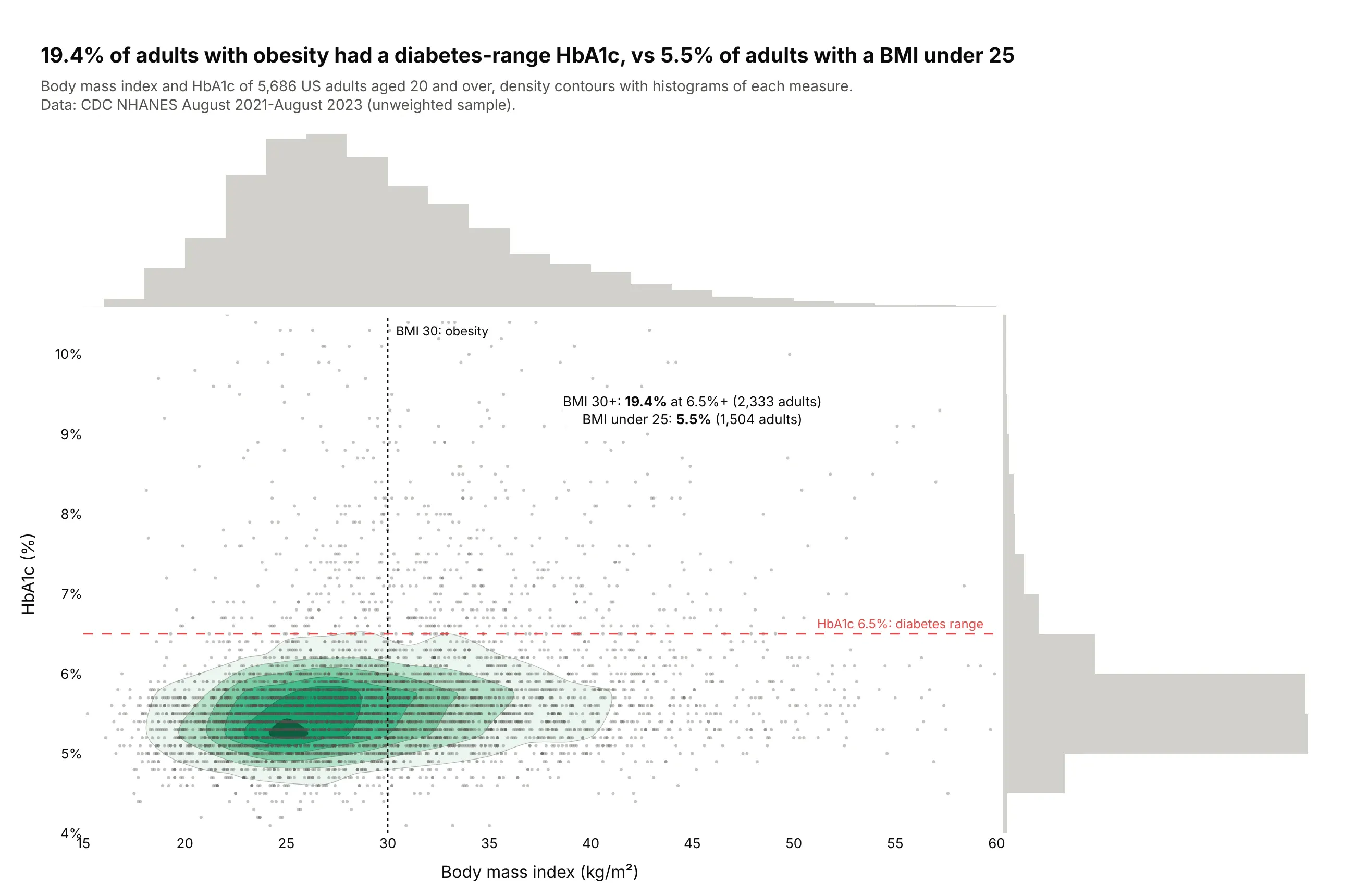
Density contour of BMI and HbA1c for 5,686 US adults with marginal histograms, faint dots for every adult, a red dashed line at HbA1c 6.5% and a dotted line at BMI 30; 19.4% of adults with a BMI of 30 or more are at 6.5% or above vs 5.5% under 25

The density of thousands of patients. In NHANES 2021-2023, 19.4% of adults with a BMI of 30 or more had an HbA1c in the diabetes range, against 5.5% of adults with a BMI under 25, and the contours show where most of the 5,686 adults sit. Data: CDC NHANES August 2021-August 2023, unweighted.

A short history

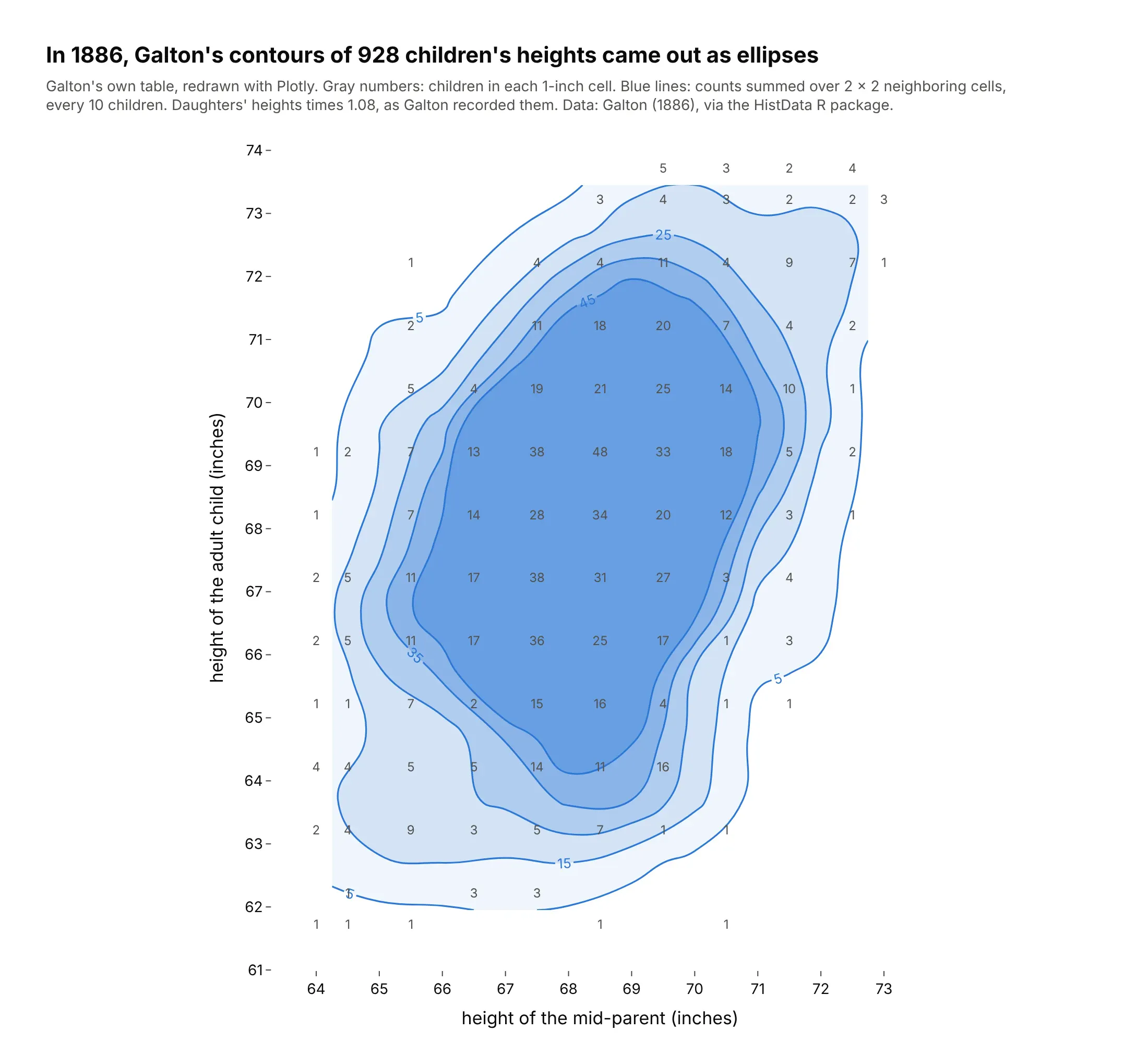
Edmond Halley's 1701 chart of the Atlantic drew lines of equal magnetic declination, Philippe Buache drew depth contours of the English Channel in 1752, and Alexander von Humboldt's 1817 isotherms gave lines of equal temperature their name, as Michael Friendly's brief history of data visualization recounts. In 1886 Francis Galton contoured a table of 928 adult children's heights against their parents' and found the lines were ellipses, which led him to regression and correlation. Here is his table redrawn with Plotly:

Galton's 1886 table of 928 adult children's heights against their mid-parent's height, redrawn with Plotly: the count in each 1-inch cell in gray, with blue contour lines every 10 children over counts summed in 2 x 2 neighboring cells, forming tilted ovals centered near 68-69 inches

Alternatives to a contour plot

Contour plots get used for two kinds of data, a grid of values and a cloud of points, so here are both, each drawn every way we discuss below. Some are better for the question, some worse, some just different:

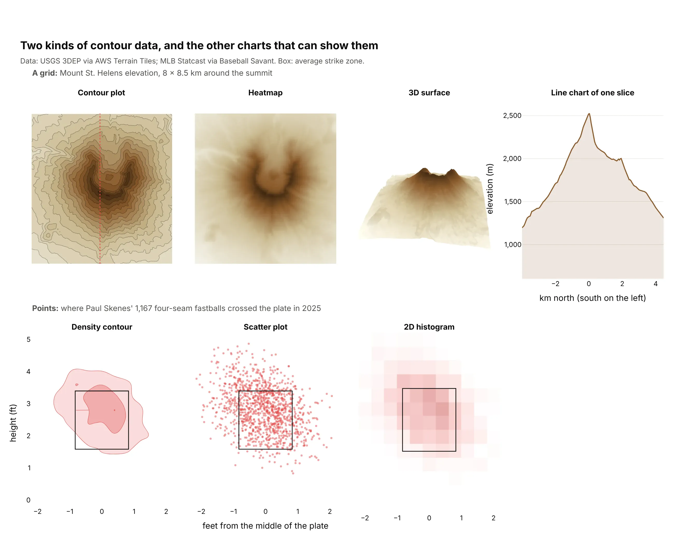
Two kinds of contour data drawn seven ways. Top row, the Mount St. Helens elevation grid as a filled contour plot, a heatmap, a 3D surface and a line chart of the north-south slice through the highest cell. Bottom row, Paul Skenes' 1,167 four-seam fastballs in 2025 as a density contour, a scatter plot and a 2D histogram on the same 0.4 ft bins, each with the strike zone drawn

Heatmap (better when the cells are the data). A heatmap colors every cell exactly as measured, so it keeps outliers, noisy values and categorical axes that contours would smooth over. It makes slope and shape harder to read. See our heatmap guide.
3D surface (different). A surface shows the shape at a glance and can be rotated in an interactive chart, but in a static image the values behind a ridge are hidden and none of them can be read off an axis.
Line chart of one slice (better for exact values along a line). People read position on a common scale more accurately than color, as Cleveland and McGill (1984) measured. The north-south profile shows the ground dropping 553 m from the rim to the crater floor at 1,973 m, but only along that one line.
Scatter plot (better for a few hundred points). Every point and every outlier stays visible. Past a thousand or so the dots overlap, and the scatter can't show where they are densest.
2D histogram (works too). It uses the same bins as a density contour and shows the counts exactly, with no smoothing, at the cost of a blocky picture. In Plotly it's go.Histogram2d, and switching to go.Histogram2dContour takes one word.

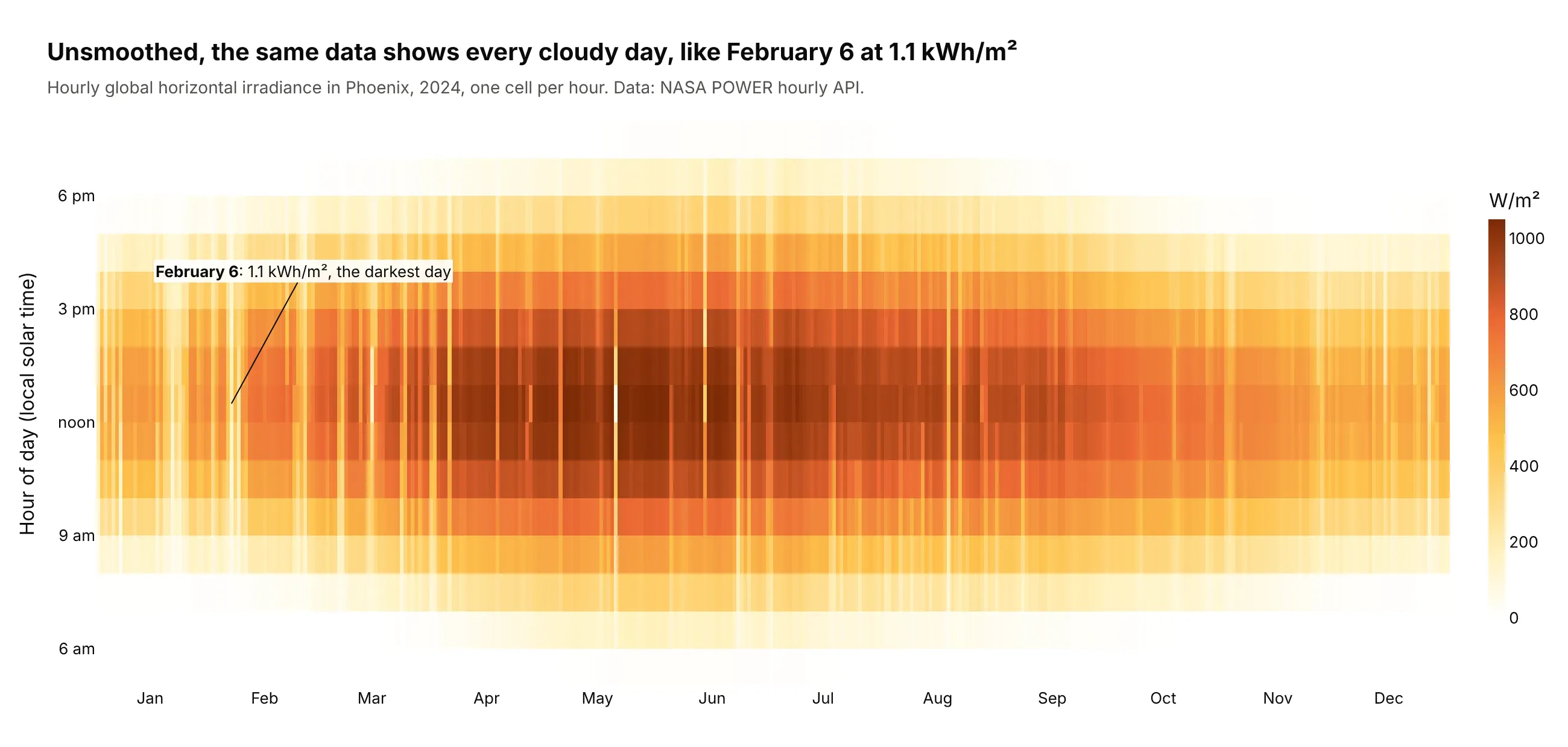
Here's where the heatmap wins. Smoothed into contours, a year of hourly sunlight in Phoenix is a clean dome (example 3 below), while the unsmoothed heatmap shows every cloudy day the contours hide, like February 6 at 1.1 kWh/m²:

Heatmap of hourly solar irradiance in Phoenix in 2024 without smoothing, with pale vertical streaks for cloudy days and February 6 labeled at 1.1 kWh/m²

How to make a contour plot

With AI

ChatGPT, Claude Code, GitHub Copilot, Cursor and other AI tools are excellent at writing Plotly code. Name Plotly in the prompt, describe the grid and the levels you want, and list the checks:

Make a plotly contour plot from grid.csv (columns: x, y, value; one row per grid point).

- Pivot to a 2D array (rows = y, columns = x) and draw go.Contour with coloring="fill".
- Levels: start, end and size set explicitly (not ncontours), at round values.
- A second go.Contour trace with coloring="none", showlabels=True labels every 5th level.
- line.smoothing=1; missing cells stay NaN (never 0); equal axis scaling if x and y share units.
- Sequential single-hue colorscale; Inter font, white background, title with the takeaway.
- Check: print the grid shape, the number of NaN cells and the min and max value,
  and confirm the levels cover that range.

The last check matters because levels outside the data range draw nothing, and a grid that didn't pivot cleanly (duplicate x-y pairs) fails without an error.

With Plotly Studio

Plotly Studio is a desktop app where you point an AI at a dataset and it builds charts and a Dash app around your questions. Ask for a contour plot by describing the grid and the levels:

Show a filled contour plot of sea surface temperature with longitude on x and latitude on y, isotherms every 1 °C on a blue-to-red scale, the 15 °C line in black, and land in light gray. Add a date picker to switch between days.

Make a contour plot in Python or JavaScript

This is the code AI tools write under the hood. In Python, go.Contour takes a grid, here pivoted from a long table of elevations, and a second trace labels every 500 m:

import pandas as pd
import plotly.graph_objects as go

url = ("https://upwell.pfeg.noaa.gov/erddap/griddap/etopo180.csv?"
       "altitude%5B(36.0):1:(36.4)%5D%5B(-112.4):1:(-111.8)%5D")
df = pd.read_csv(url, skiprows=[1])  # Grand Canyon elevation, NOAA ETOPO1
g = df.pivot(index="latitude", columns="longitude", values="altitude")

fig = go.Figure(go.Contour(x=g.columns, y=g.index, z=g.values, colorscale="earth",
                           contours=dict(start=500, end=3000, size=100)))
fig.add_trace(go.Contour(x=g.columns, y=g.index, z=g.values, showscale=False,
                         contours=dict(start=500, end=3000, size=500, coloring="none", showlabels=True),
                         line=dict(color="black", width=1.5)))
fig.update_yaxes(scaleanchor="x", scaleratio=1.24)  # 1 / cos(36.2°) keeps the map unstretched
fig.show()

For points, Plotly Express makes a density contour in one line of code:

import pandas as pd
import plotly.express as px

url = ("https://earthquake.usgs.gov/fdsnws/event/1/query?format=csv&starttime=2024-01-01&endtime=2025-01-01"
       "&minmagnitude=2.5&minlatitude=32&maxlatitude=42&minlongitude=-125&maxlongitude=-114")
px.density_contour(pd.read_csv(url), x="longitude", y="latitude").show()

To make a contour chart in JavaScript, plotly.js takes the same x, y and a 2D z. This is Galton's 1886 table from the history section, children's height in rows and mid-parent's height in columns:

<div id="chart"></div>
<script src="https://cdn.plot.ly/plotly-4.1.1.min.js"></script>
<script>
  Plotly.newPlot("chart", [{
    type: "contour",
    x: [64, 64.5, 65.5, 66.5, 67.5, 68.5, 69.5, 70.5, 71.5, 72.5, 73],
    y: [61.7, 62.2, 63.2, 64.2, 65.2, 66.2, 67.2, 68.2, 69.2, 70.2, 71.2, 72.2, 73.2, 73.7],
    z: [[1, 1, 1, 0, 0, 1, 0, 1, 0, 0, 0], [0, 1, 0, 3, 3, 0, 0, 0, 0, 0, 0],
        [2, 4, 9, 3, 5, 7, 1, 1, 0, 0, 0], [4, 4, 5, 5, 14, 11, 16, 0, 0, 0, 0],
        [1, 1, 7, 2, 15, 16, 4, 1, 1, 0, 0], [2, 5, 11, 17, 36, 25, 17, 1, 3, 0, 0],
        [2, 5, 11, 17, 38, 31, 27, 3, 4, 0, 0], [1, 0, 7, 14, 28, 34, 20, 12, 3, 1, 0],
        [1, 2, 7, 13, 38, 48, 33, 18, 5, 2, 0], [0, 0, 5, 4, 19, 21, 25, 14, 10, 1, 0],
        [0, 0, 2, 0, 11, 18, 20, 7, 4, 2, 0], [0, 0, 1, 0, 4, 4, 11, 4, 9, 7, 1],
        [0, 0, 0, 0, 0, 3, 4, 3, 2, 2, 3], [0, 0, 0, 0, 0, 0, 5, 3, 2, 4, 0]],
    colorscale: "Blues",
    contours: { start: 5, end: 45, size: 10, showlabels: true },
    line: { smoothing: 1.3 }
  }], { xaxis: { title: { text: "Mid-parent height (in)" } },
        yaxis: { title: { text: "Child height (in)" } } });
</script>

Without contours.start, end and size, Plotly picks the levels itself, and ncontours only sets a maximum that it rounds to nice steps.

Share it

Every Plotly chart has a Share chart button (the cloud icon in its toolbar) that uploads it to Plotly Cloud and gives you a link. Only you can see it until you change its visibility.

For a live app, put the chart in a Dash app and publish it with the Plotly Cloud CLI. Coding agents can run these commands for you:

pip install "dash[cloud]"
plotly user login
plotly app publish

If your data has to stay in your own cloud or data center, publish to Dash Enterprise instead.

Dos and don'ts

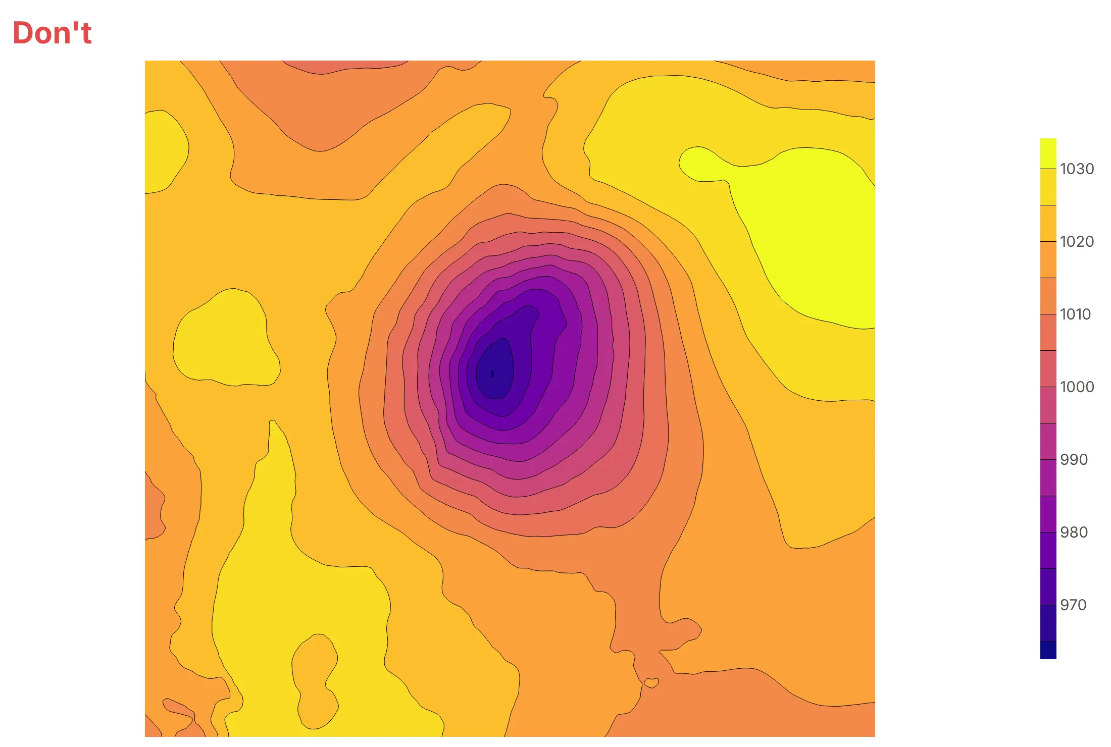
Plotly's defaults are made for exploring a grid quickly. For a published chart, most of the work is choosing the levels and adding the reference that tells readers where they are. Here is the same pressure field from the 1993 storm both ways.

Don't publish the default colorscale, levels Plotly picked for you and no map, because nobody can tell this is a storm over the East Coast:

The 1993 storm's sea-level pressure as a default filled contour plot with a yellow-to-purple colorscale, automatic levels and no map

Do draw isobars every 4 hPa, the step meteorologists use, label them, put them over coastlines and mark the low:

The same pressure field as a weather map: purple to gray isobars every 4 hPa, labeled, over coastlines and state lines, with a red L at the low near Philadelphia

Pick contours.coloring for what else is on the chart

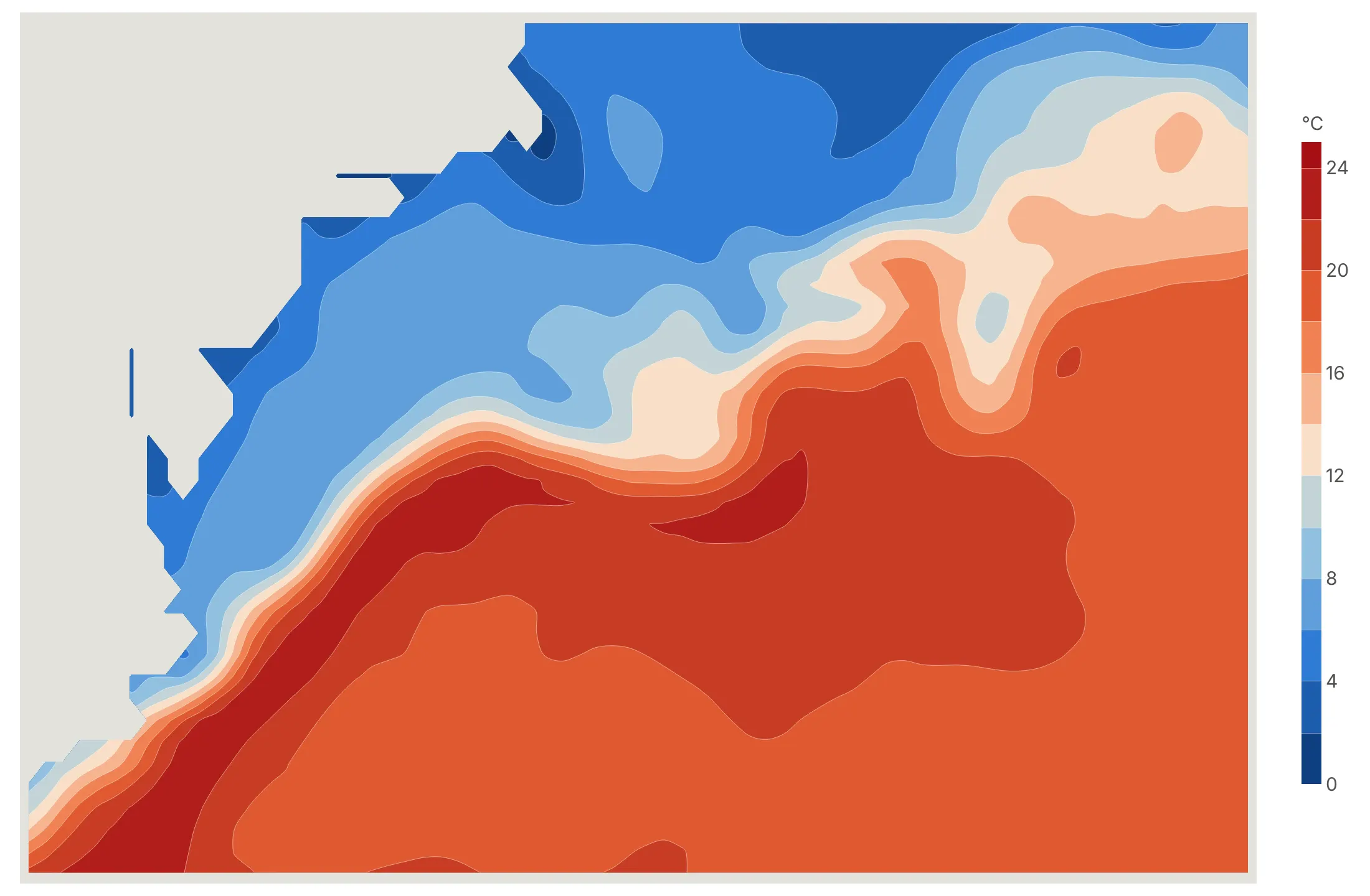
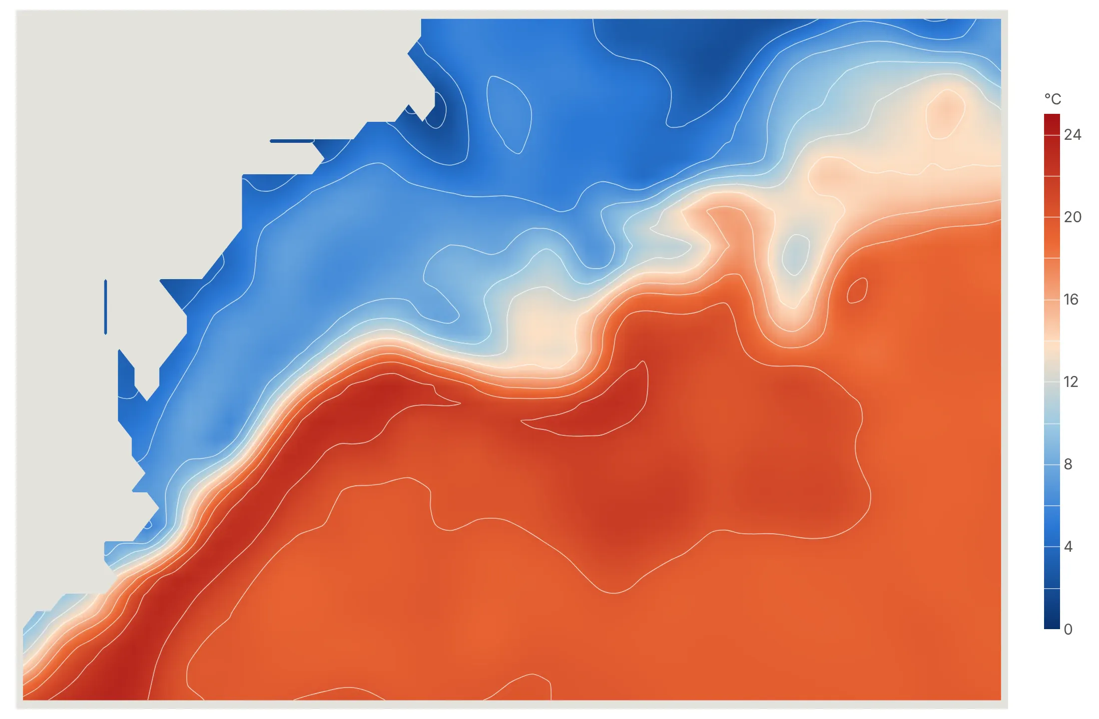
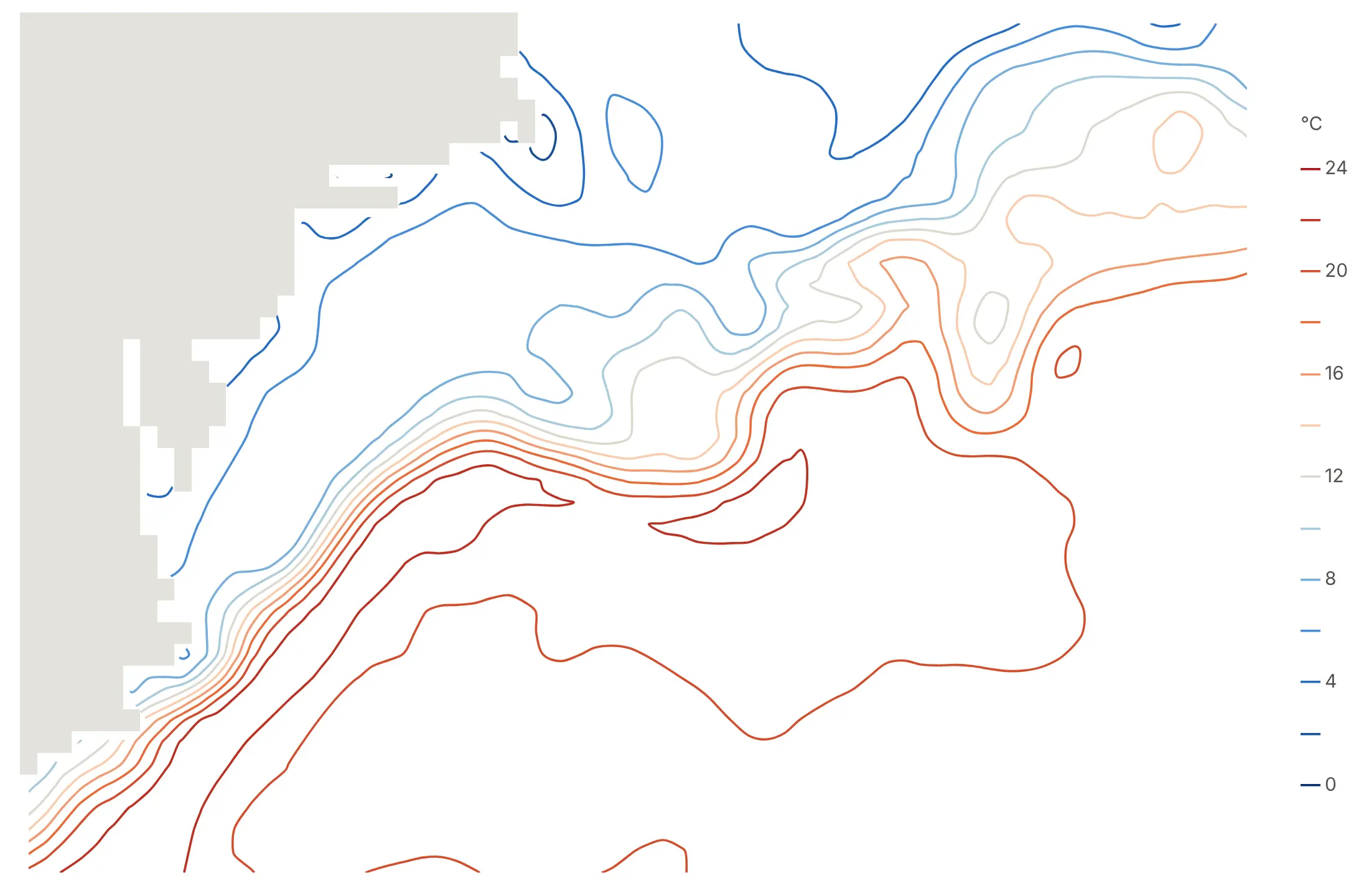
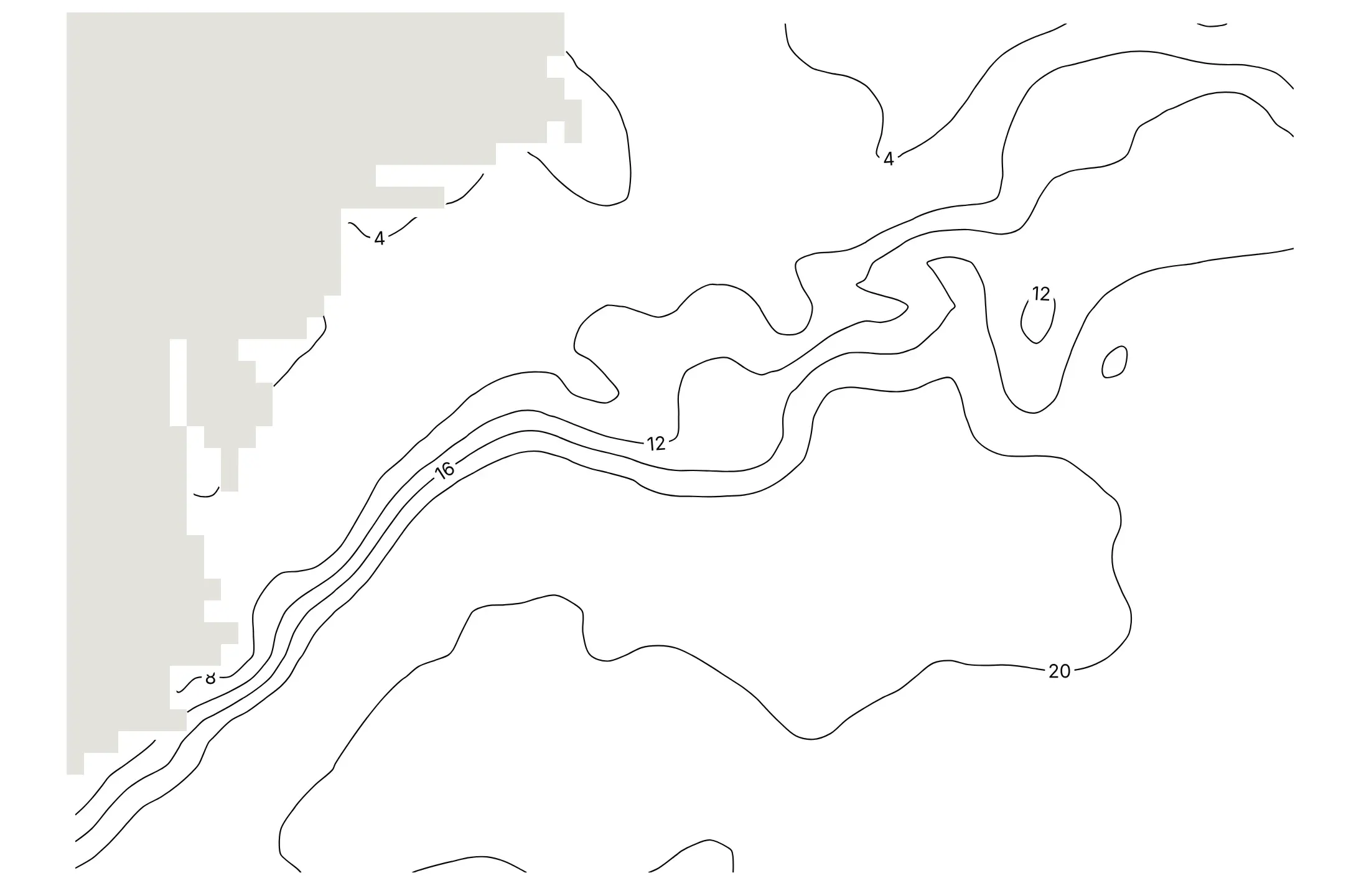
contours.coloring decides what fills the space between the lines. Here are the four options on the Gulf Stream's sea surface temperature on February 15, 2025.

fill colors each band between two levels, so values read like a stepped scale. It's the right default when the contour is the only layer.

Sea surface temperature off the US East Coast as filled contour bands every 2 °C, blue in the north and red in the Gulf Stream, with land in gray

heatmap shades smoothly between levels and keeps the lines on top for exact values, as in the wind map above.

The same sea surface temperature with smooth heatmap shading and thin white contour lines every 2 °C

lines draws only the lines, each in its level's color, which leaves room for a map or points underneath.

The same sea surface temperature drawn as colored contour lines only, blue to red, every 2 °C, over a white ocean and gray land

none with labels gives the black-and-white look of a printed map, which works best over another colored layer.

The same sea surface temperature as black contour lines every 4 °C with labels and no fill, ocean in white and land in gray

Set the levels yourself

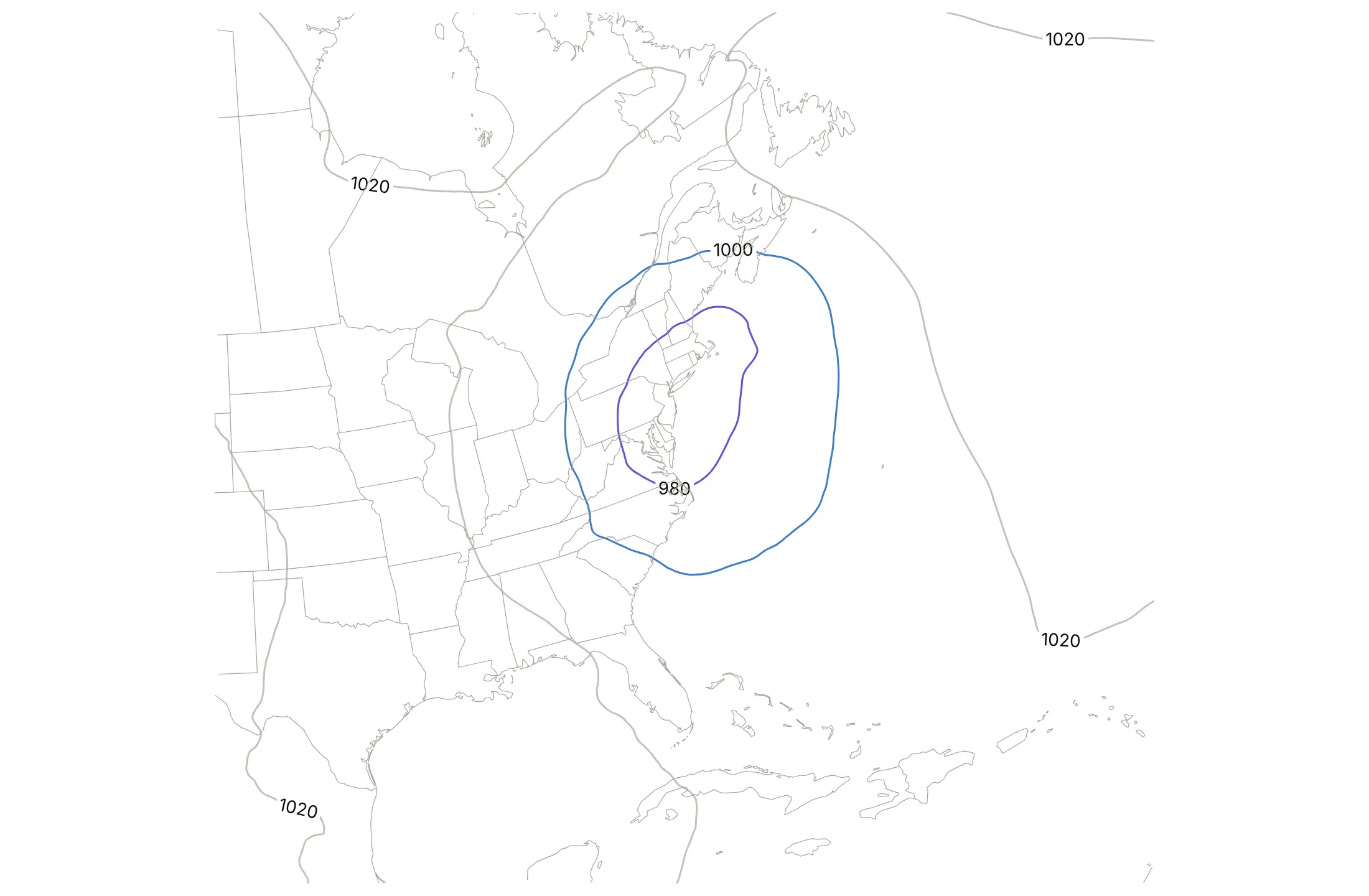
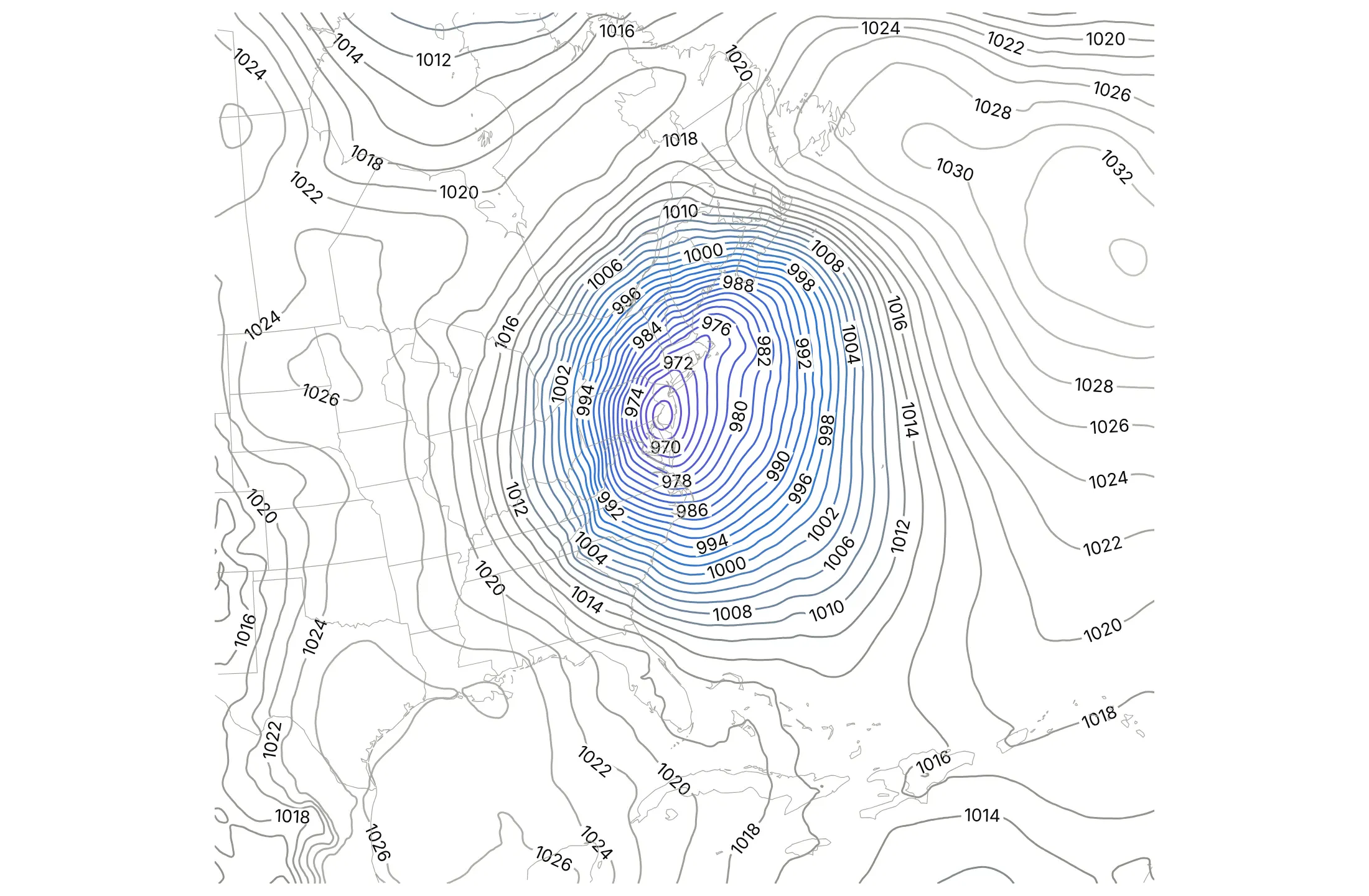
ncontours is a maximum that Plotly rounds to nice steps, so the same storm can come out with steps that are too coarse or too fine.

ncontours=6 gave 20 hPa steps, and the storm's structure disappears.

The 1993 storm's pressure field with ncontours=6, which Plotly turned into three isobars 20 hPa apart

ncontours=40 gave 2 hPa steps, twice as many lines as a weather map would draw, so the chart fills with lines and labels.

The same pressure field with ncontours=40, which Plotly turned into isobars every 2 hPa, with dozens of labeled lines crowded around the low

start=964, end=1040, size=4 sets exactly the 4 hPa isobars a weather service would draw.

The same pressure field with isobars every 4 hPa from 964 hPa, labeled

Checklist

Set levels with contours.start, end and size at values people use: 4 hPa isobars, 100 m of elevation, whole degrees.
Label a few index lines with a second trace that has coloring="none" and showlabels=True, as on a topographic map.
Use one hue for amounts, and a diverging scale centered with zmid for values above and below a baseline.
Keep equal scaling on maps (yaxis.scaleanchor="x", with scaleratio corrected for latitude).
Add the context readers need: coastlines, a strike zone, threshold lines.
Use a log scale for counts that span decades: contour log10(z) and relabel the colorbar.

Don't

Use a rainbow colorscale for a single quantity.
Label every level, which clutters the chart and draws more than ten times slower.
Contour noisy data without smoothing it first and saying how you smoothed it.
Fill missing cells with zero. Leave them NaN so the background shows through.

Options to customize

These are the go.Contour and go.Histogram2dContour options that matter most. The full list is in the Plotly contour reference and the contour plots documentation.

x, y, z: a 2D z with x and y vectors, or 1D columns that fall on a grid.
go.Histogram2dContour(x, y) and px.density_contour: bin points and contour the counts, for point density.
contours.coloring: fill, heatmap, lines or none. Use lines or none over a map.
contours.start, end, size: exact levels, whenever the steps carry meaning.
ncontours: the maximum number of levels, rounded to nice steps. Fine for a first look.
contours.showlabels, labelfont, labelformat: values on the lines. Use them on a few index lines only.
line.smoothing (0 to 1.3): smooths the drawn lines, which hides the stair steps of a coarse grid.
line.width, line.color: thin lines for bands, bold ones for index lines.
colorscale, zmin, zmax, zmid: the color mapping. zmid centers a diverging scale.
connectgaps: interpolates across missing cells, which is usually best left off so gaps stay visible.
histnorm, xbins, ybins, nbinsx, nbinsy: normalization and bins for density contours. Use the same bins to compare groups.
yaxis.scaleanchor, scaleratio: equal scaling for maps and for x and y in the same units.
yaxis.autorange="reversed": flips the y axis, for depth or magnitudes.
yaxis.type="log": a log axis for gridded data, such as days to expiry or bond maturities.

More contour plot examples

Ten more contour plots built from real public data, each with its source, the technique that makes it work and a prompt to rebuild it.

1. The Gulf Stream's north wall

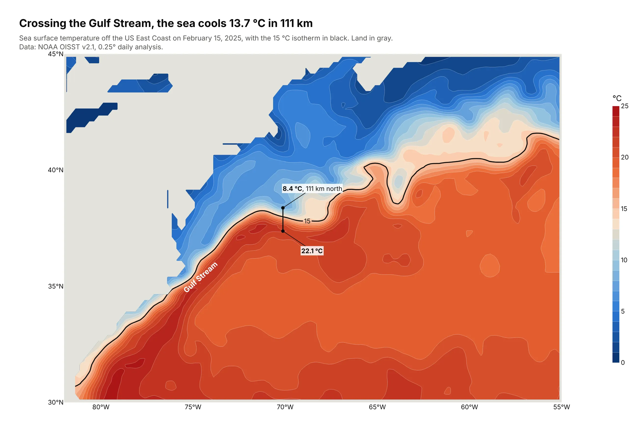
Filled contour map of sea surface temperature off the US East Coast on February 15, 2025, blue in the north and red in the Gulf Stream, with the 15 °C isotherm in black and a marked drop from 22.1 °C to 8.4 °C over 111 km at 70°W

Isotherms bunch where warm Gulf Stream water meets cold shelf water. Along 70°W on February 15, 2025, the sea surface cooled from 22.1 °C to 8.4 °C in 111 km. Data: NOAA OISST v2.1, 0.25° daily analysis.

Tip: a second trace with start=end=15 draws a single isotherm in black to trace the front.

Get the data from NOAA NCEI's Daily Optimum Interpolation SST v2.1 (AVHRR, 0.25°) file for
February 15, 2025 and shape it into a table (columns: lat, lon, sst_c) for 30-45°N, 82-55°W.

Build a plotly filled contour map, isotherms every 1 °C on a blue-to-red scale, land as a light gray
background (NaN cells). Add the 15 °C isotherm in black. Mark the temperature change across the
front along 70°W.

2. Offshore boreholes on the continental slope

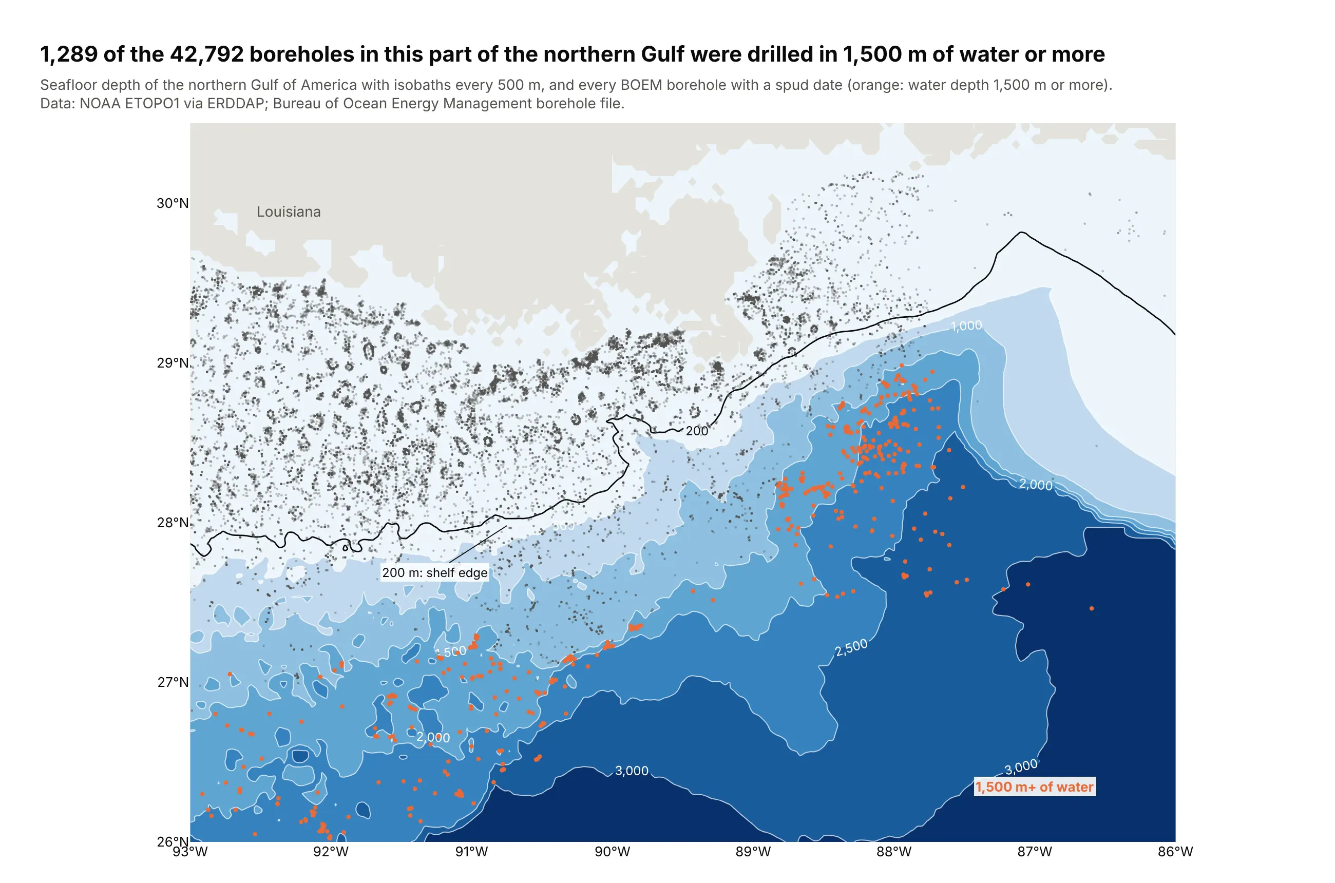
Bathymetric contour map of the northern Gulf of America with isobaths every 500 m and the 200 m shelf edge in black, 42,792 boreholes as gray dots on the shelf and 1,289 orange dots in 1,500 m of water or more

Of the 42,792 boreholes drilled in this part of the northern Gulf, 1,289 are in 1,500 m of water or more, out on the slope where the isobaths fan out. The deepest sits in 3,091 m. Data: NOAA ETOPO1 via ERDDAP; BOEM borehole file.

Tip: contours as the base layer and points on top, with the subset that matters in one color.

Get the data from NOAA's ETOPO1 relief model (ERDDAP dataset etopo180, 26-30.5°N, 93-86°W) and
BOEM's borehole file (data.boem.gov, 5010delimit.zip) and shape them into two tables (columns:
lat, lon, depth_m) and (columns: lat, lon, water_depth_m, spud_year).

Build a plotly filled contour map of depth with labeled isobaths every 500 m, land as NaN, the 200 m
line in black, and the boreholes as dots, orange for 1,500 m of water or more.

3. A year of sunlight in Phoenix

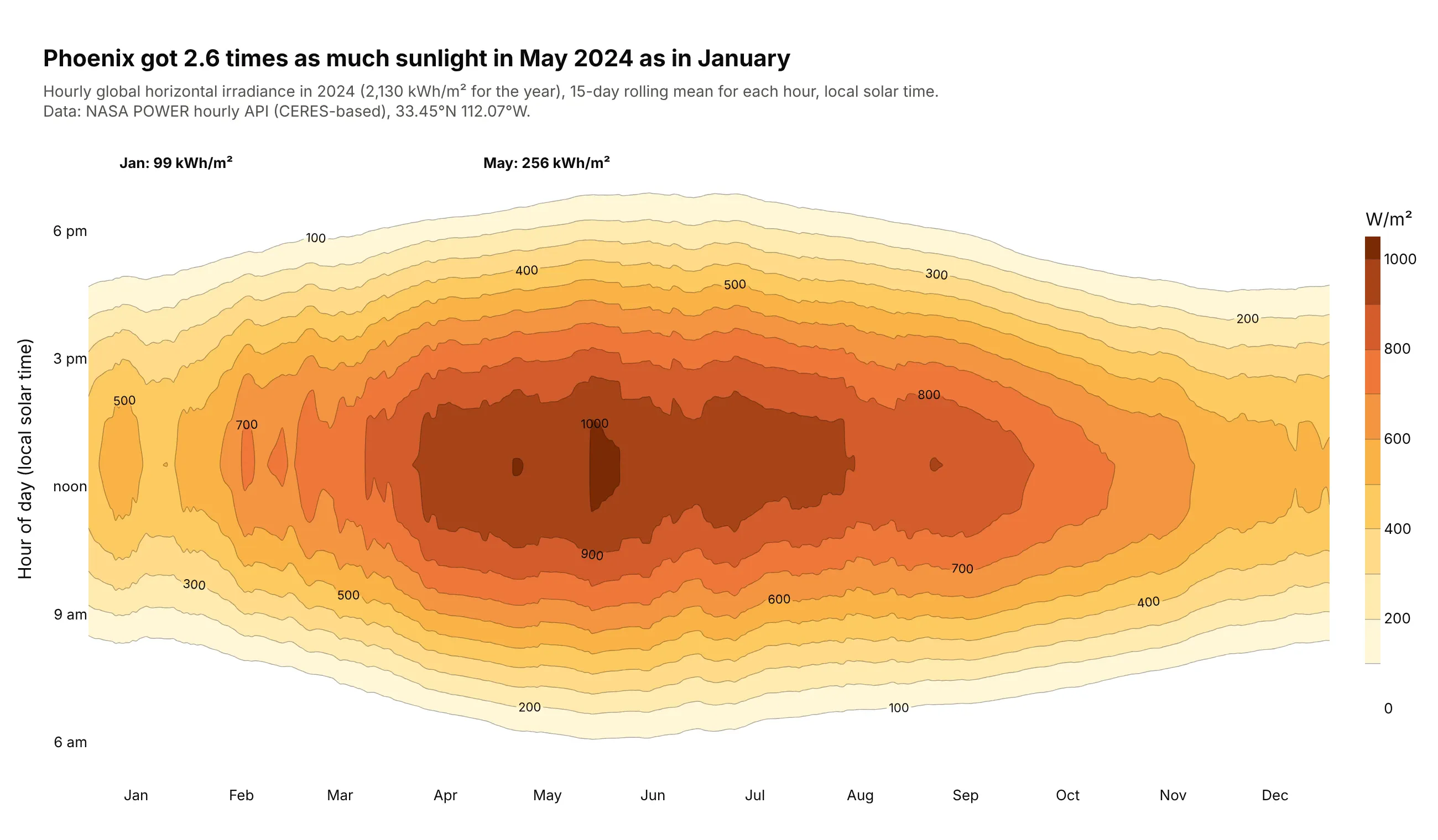
Filled contour plot of hourly solar irradiance in Phoenix in 2024 by day of year and hour, a dome from about 6 am to 6 pm that is widest and darkest from April to August, with January at 99 kWh/m² and May at 256 kWh/m²

Phoenix got 2.6 times as much sunlight in May 2024 (256 kWh/m²) as in January (99 kWh/m²), for 2,130 kWh/m² over the year. The dome's width is the length of the day. Data: NASA POWER hourly API, 33.45°N 112.07°W.

Tip: smooth each hour with a 15-day rolling mean before contouring, and say so in the subtitle. The unsmoothed heatmap is in the alternatives section above.

Get the data from the NASA POWER hourly point API (ALLSKY_SFC_SW_DWN, community RE, local solar time)
for 33.45°N 112.07°W, 2024 and shape it into a table (columns: date, day_of_year, hour, ghi_wm2).

Pivot to hour x day of year, smooth each hour with a 15-day centered rolling mean, and build a plotly
filled contour plot with levels every 100 W/m², a white-to-brown scale and month names on x.

4. The S&P 500 implied volatility surface

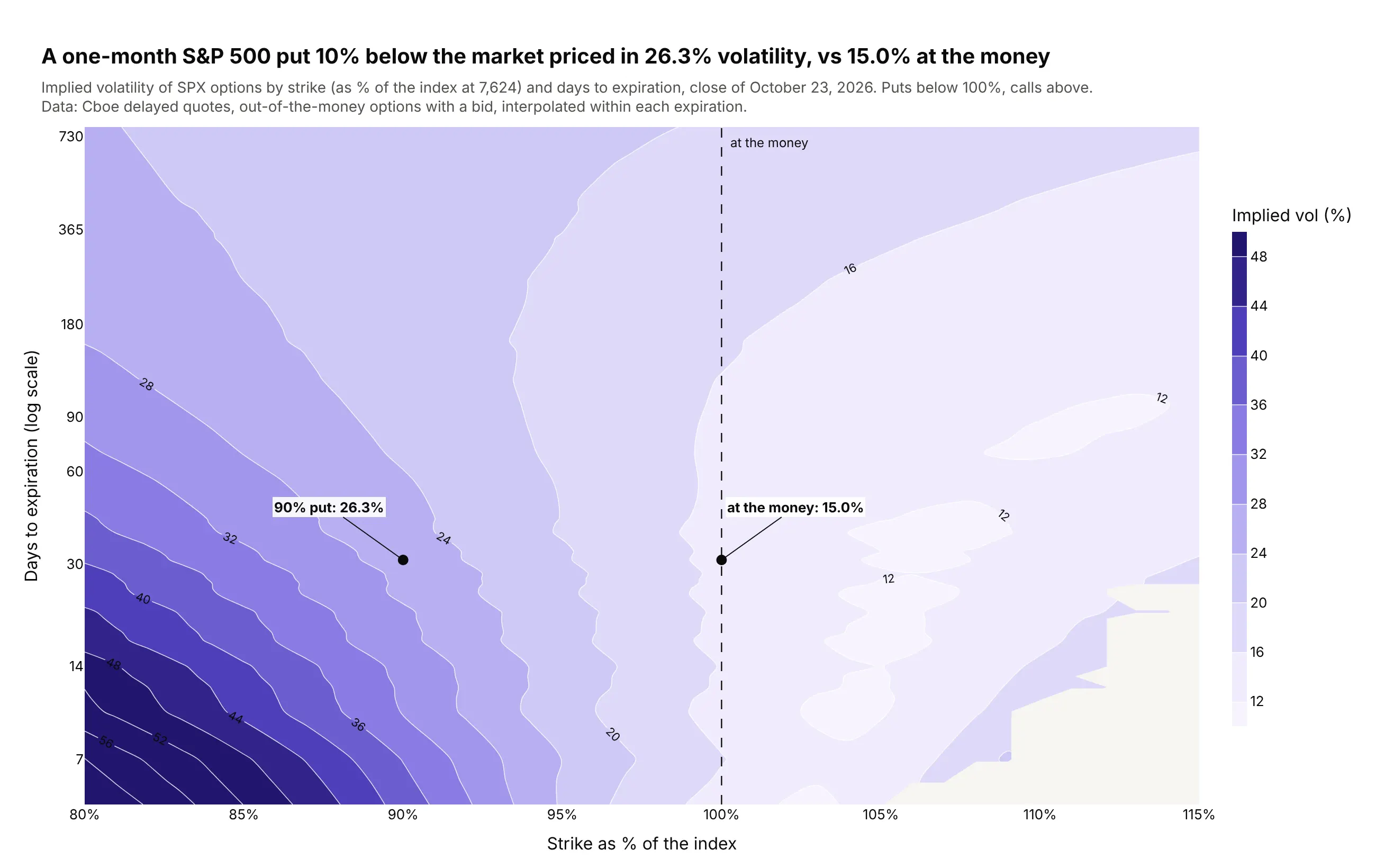
Filled contour plot of SPX implied volatility by strike from 80% to 115% of the index and days to expiration on a log scale, labeled every 4 points, dark purple for short-dated puts and pale for calls, with a 31-day put at 90% priced at 26.3% and the at-the-money option at 15.0%

At the October 23, 2026 close, a one-month S&P 500 put 10% below the market priced in 26.3% volatility, against 15.0% at the money. The contours fan out at short expirations, where the skew is steepest. Data: Cboe delayed quotes, SPX and SPXW options.

Tip: interpolate each expiration onto a common strike grid only inside its quoted strikes, and use a log axis for days.

Get the data from Cboe's delayed quotes API (cdn.cboe.com/api/global/delayed_quotes/options/_SPX.json)
and shape it into a table (columns: expiry, days, type, strike, moneyness, iv) of out-of-the-money
options with a bid.

For each expiration, interpolate iv onto moneyness 0.80-1.15 in 1% steps with np.interp, NaN outside
the quoted range. Build a plotly filled contour plot, days on a log y axis, lines every 4 vol points,
labeled. Annotate the 90% put and the at-the-money option near 30 days.

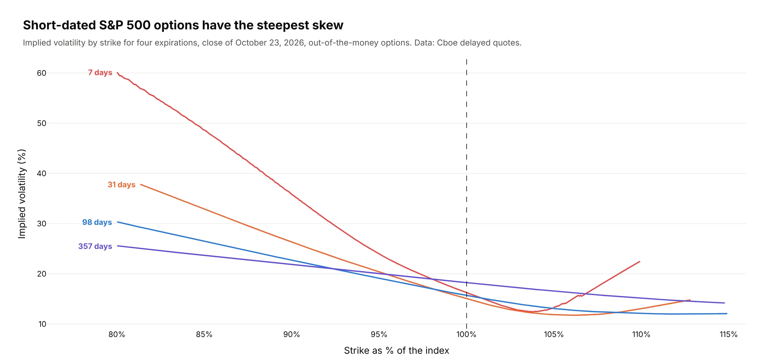
Another way to see it: smile lines for four expirations show the same skew as slopes, and the 7-day smile climbs to about 60% at 80% of the index. Traders read smiles more precisely, but the contour shows every expiration at once.

Implied volatility smiles for 7, 31, 98 and 357 days, the 7-day line rising steeply to about 60% at 80% of the index and the 357-day line nearly flat

5. The shape of the Treasury yield curve since 1990

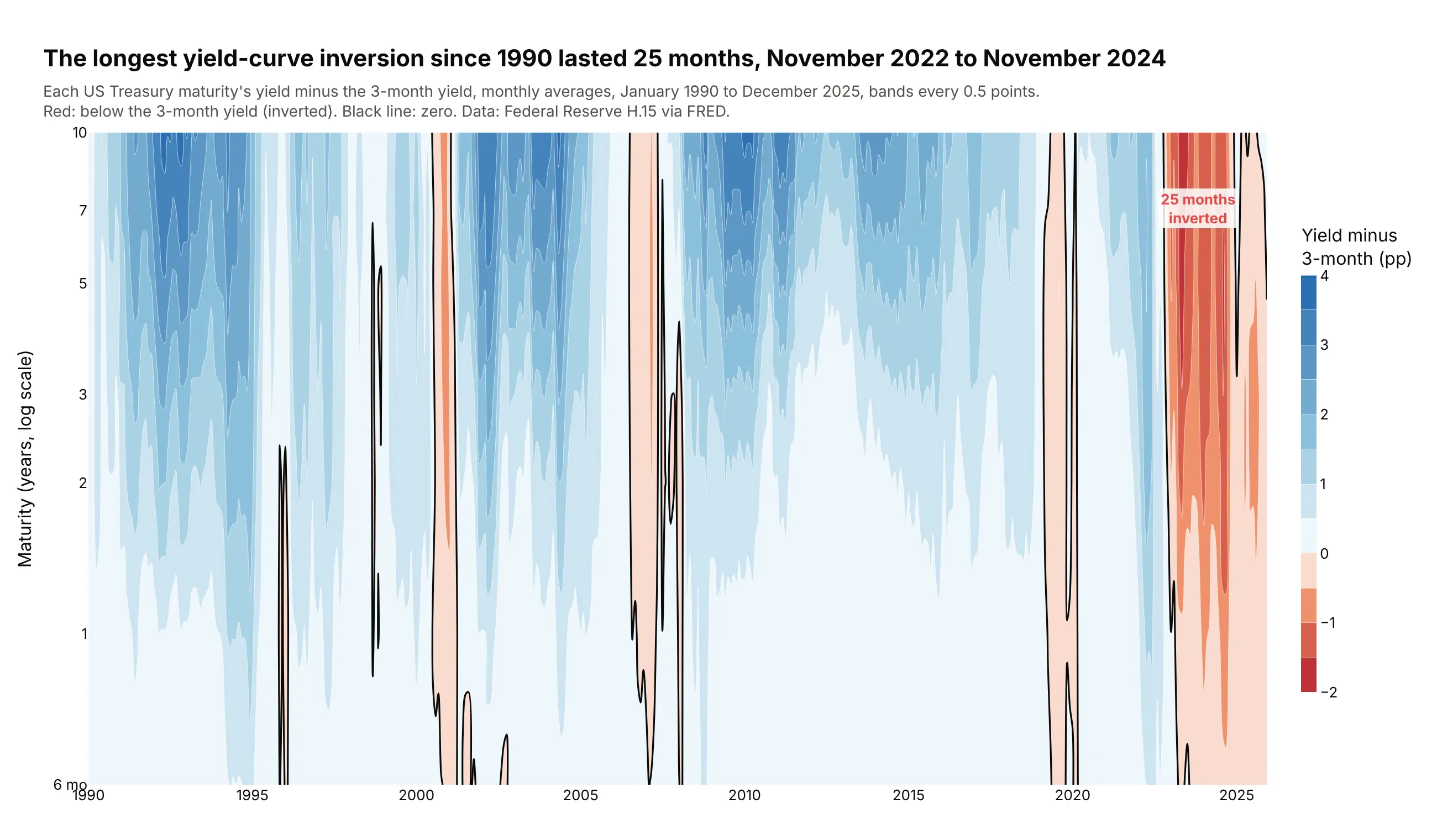
Contour plot of each Treasury maturity's yield minus the 3-month yield, 1990-2025, by maturity from 6 months to 10 years, blue when the curve slopes up and red when inverted, with a black zero line and the 25-month inversion of 2022-2024 marked

The longest yield-curve inversion since 1990 lasted 25 months, from November 2022 to November 2024, by monthly averages of the 10-year and 3-month yields. Contouring each yield minus the 3-month yield shows every inversion as a red block. Data: Federal Reserve H.15 via FRED.

Tip: contour the difference, not the level, with a diverging scale and zmid=0.

Get the data from FRED (DGS3MO, DGS6MO, DGS1, DGS2, DGS3, DGS5, DGS7, DGS10) and shape it into a
table (columns: month, maturity_years, yield_pct) of monthly averages, 1990-2025.

Subtract the 3-month yield from each maturity and build a plotly filled contour plot: months on x,
maturity on a log y axis, a red-white-blue scale with zmid=0, bands every 0.5 points, and a second
trace drawing only the zero line in black. Find the longest run of inverted months.

6. Tomorrow's S&P 500 move, given today's VIX

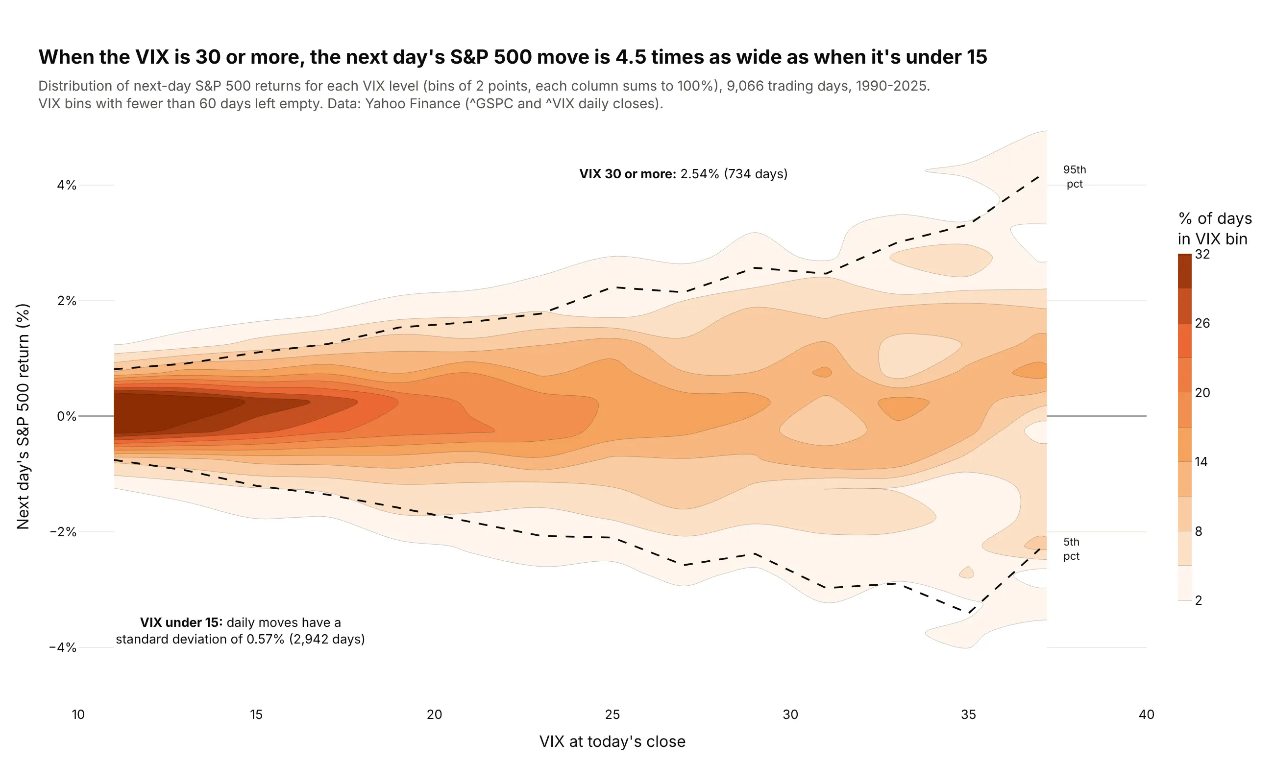
Conditional density contour of next-day S&P 500 returns by VIX level, 1990-2025, narrow and dark at low VIX and fanning out at high VIX, with dashed 5th and 95th percentile lines

When the VIX closed at 30 or more, the next day's S&P 500 return had a standard deviation of 2.54%, 4.5 times the 0.57% when it closed under 15. The contours fan out as fear rises. Data: Yahoo Finance daily closes of ^GSPC and ^VIX, 1990-2025.

Tip: normalize each VIX column to 100% so rare high-VIX days are as visible as calm ones.

Get the data from Yahoo Finance's chart API (daily closes of ^GSPC and ^VIX, 1990-2025) and shape it
into a table (columns: date, vix, next_return_pct).

Build a 2D histogram with np.histogram2d (VIX bins of 2 points, return bins of 0.5%), divide each VIX
column by its total, drop columns with under 60 days, and draw it with go.Contour. Overlay the 5th and
95th percentile of returns per VIX bin as dashed lines.

7. Phase 1 vs Phase 3 trials

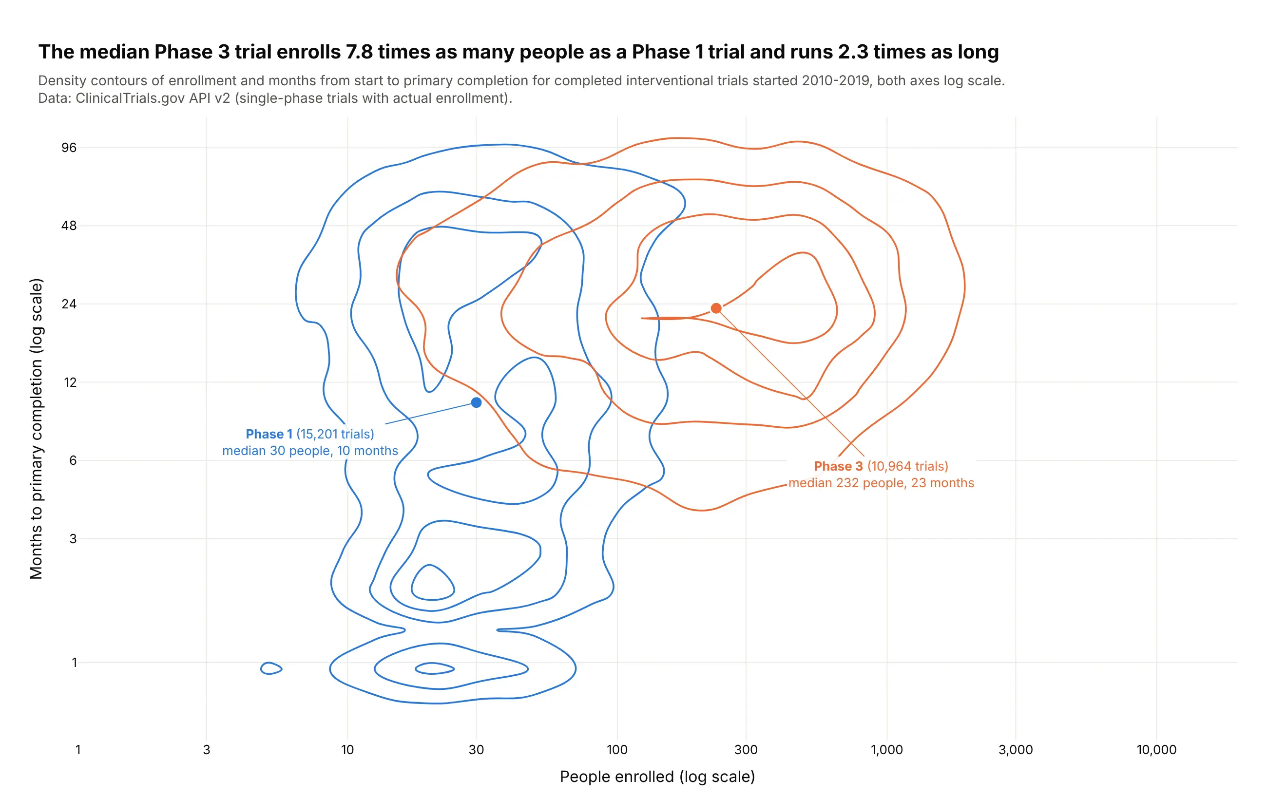
Two sets of density contour lines on log axes of enrollment and months to primary completion, blue for 15,201 Phase 1 trials centered on 30 people and 10 months, orange for 10,964 Phase 3 trials centered on 232 people and 23 months

The median Phase 3 trial started in 2010-2019 enrolled 7.8 times as many people as a Phase 1 trial (232 vs 30) and ran 2.3 times as long to primary completion (23 vs 10 months). Data: ClinicalTrials.gov API v2, 26,165 completed trials.

Tip: log-transform both axes before binning, then relabel the ticks, because histogram bins are linear.

Get the data from the ClinicalTrials.gov API v2 (completed interventional Phase 1 or Phase 3 trials
started 2010-2019) and shape it into a table (columns: nct_id, phase, enrollment,
months_to_primary).

Build a plotly figure with one go.Histogram2dContour per phase on log10(enrollment) and
log10(months), histnorm="probability", the same bins, coloring="lines" in one color per phase,
ticks relabeled as real numbers, and a marker at each phase's medians.

8. The Tonga slab, drawn by 32,000 earthquakes

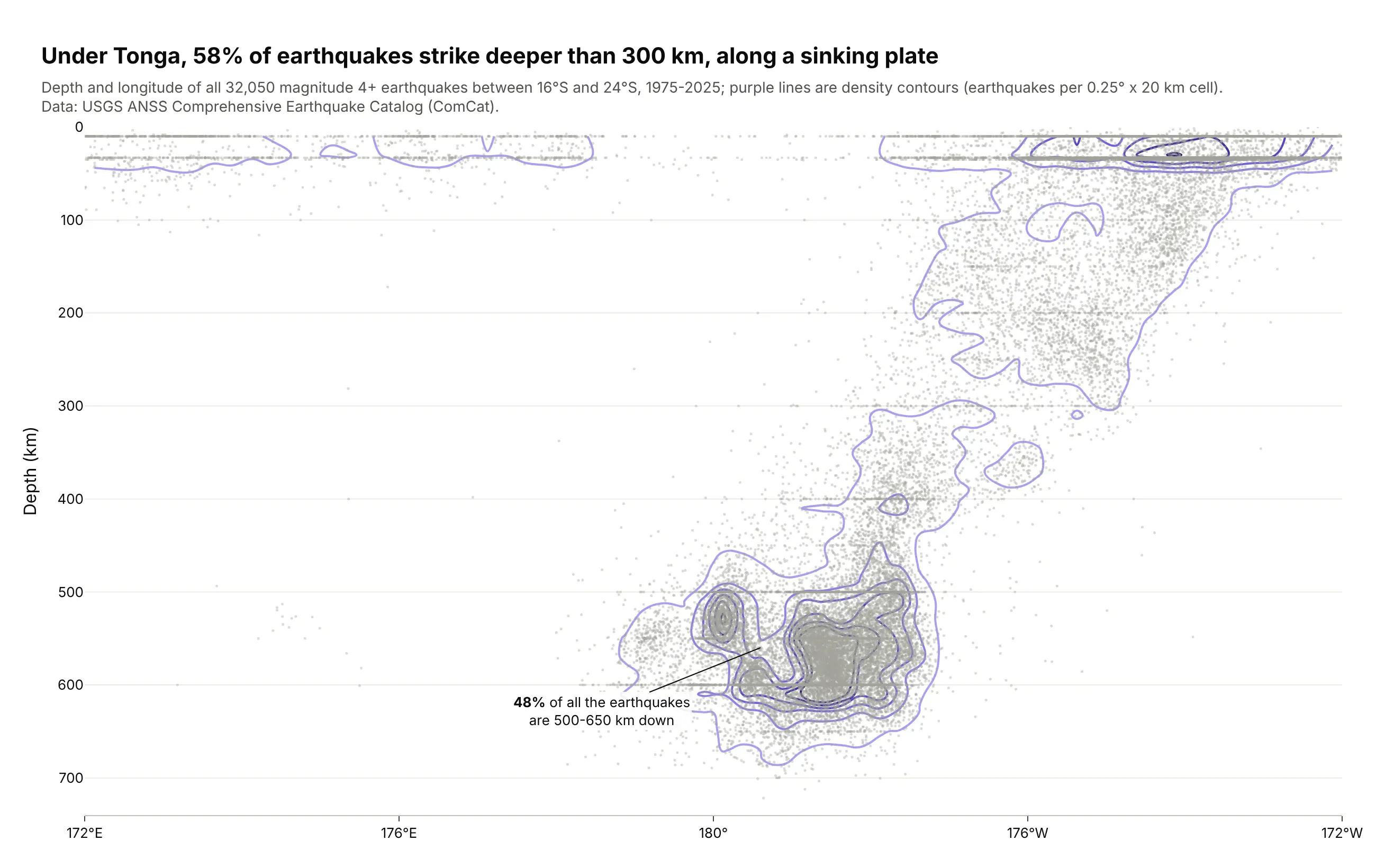
Cross-section of 32,050 magnitude 4+ earthquakes under Tonga by longitude and depth, gray dots with purple density contours along a band dipping west from the surface to about 700 km

Under Tonga, 58% of magnitude 4+ earthquakes since 1975 struck deeper than 300 km, along the Pacific plate sinking westward. The densest contours sit 500-650 km down, where 48% of all events cluster. Data: USGS ANSS Comprehensive Earthquake Catalog.

Tip: density contour lines over faint dots show both the outliers and the core.

Get the data from the USGS earthquake catalog (earthquake.usgs.gov/fdsnws/event/1/query, magnitude
4+, 1975-2025, 24-16°S, 172°E-172°W) and shape it into a table (columns: time, lat, lon_e, depth_km, mag)
with longitude in 0-360.

Build a plotly cross-section: every event as a small gray dot, then go.Histogram2dContour with
coloring="lines", bins of 0.25° x 20 km, depth axis reversed. Title: the share deeper than 300 km.

9. The Hertzsprung-Russell diagram of 263,609 stars

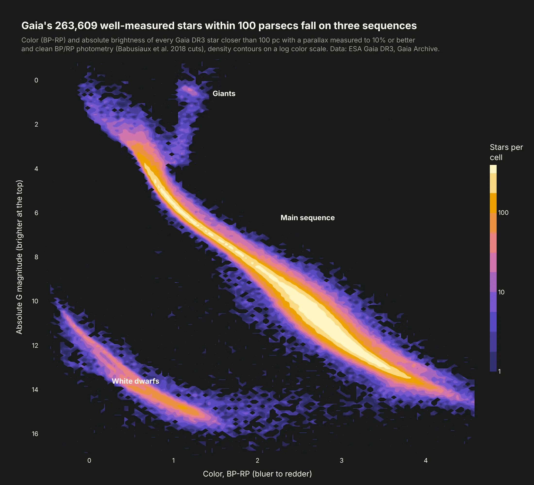
Hertzsprung-Russell diagram of 263,609 Gaia DR3 stars within 100 parsecs as log-scaled density contours on a dark background, with a bright main sequence, a separate white dwarf sequence and a giant branch

Gaia's 263,609 well-measured stars within 100 parsecs fall on three sequences: the main sequence, the white dwarfs and the giants. Counts range from 1 to 172 per cell, so only a log scale shows all three. Data: ESA Gaia DR3 via the Gaia Archive.

Tip: aggregate on the server with an ADQL GROUP BY, then contour log10(count) with a relabeled colorbar.

Get the data from the ESA Gaia Archive TAP service (gaiadr3.gaia_source, parallax > 10 mas,
parallax_over_error > 10, BP/RP flux_over_error > 10, Babusiaux et al. excess-factor cut), binned on
the server with GROUP BY into a table (columns: bp_rp, m_g, stars) of 0.02 x 0.05 mag cells.

Build a plotly go.Contour of log10(stars), magnitude axis reversed, colorbar ticks 1, 10, 100,
empty cells NaN, dark background. Label the main sequence, white dwarfs and giants.

10. Where Paul Skenes threw his pitches

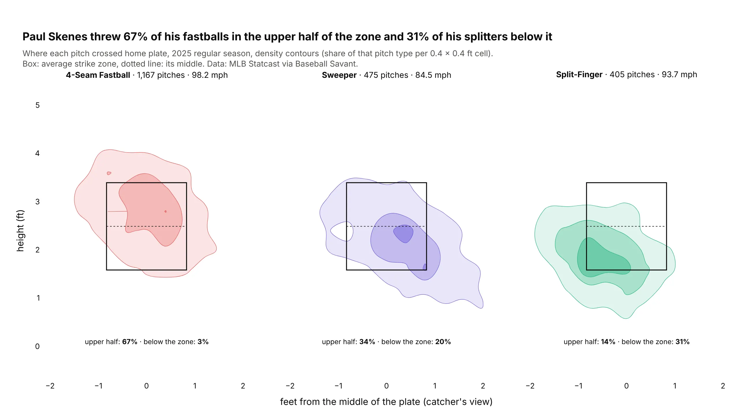
Three density contour panels of where Paul Skenes' 2025 four-seam fastballs, sweepers and splitters crossed home plate, with the strike zone drawn; 67% of fastballs were in the upper half of the zone and 31% of splitters below it

In 2025, Paul Skenes threw 67% of his 1,167 four-seam fastballs in the upper half of the strike zone and 31% of his 405 splitters below it. The sweeper runs down and away to his glove side. Data: MLB Statcast via Baseball Savant.

Tip: small multiples with the same bins, levels and color range, so the panels compare directly.

Get the data from Baseball Savant's Statcast search CSV (pitcher 694973, 2025 regular season) and
shape it into a table (columns: game_date, pitch_name, release_speed, plate_x, plate_z, sz_top, sz_bot).

Build a plotly figure with make_subplots, one go.Histogram2dContour per pitch type (fastball,
sweeper, splitter), histnorm="probability", bins of 0.4 ft, the same levels, filled in each pitch's
color, the average strike zone as a rectangle, equal axis scaling.

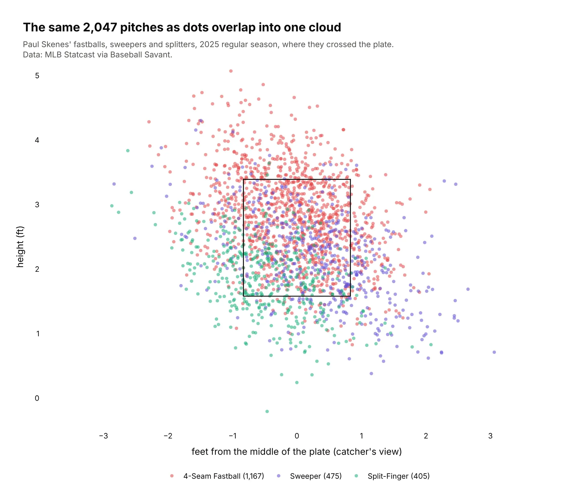
Another way to see it: the same 2,047 pitches as dots overlap into one cloud, which is why pitch charts use contours.

Scatter plot of 2,047 Paul Skenes pitches colored by type, overlapping inside and around the strike zone