Chris Parmer

October 24, 2026

Hexbin Plots - A Complete Guide (with 13 Examples)

TL;DR

A hexbin plot splits the x-y plane into hexagons and colors each one by how many points fall inside it, so a scatter plot of millions of points becomes a readable map of where the data is dense.
Hexbin plots are also known as hexagonal binning plots and hexagonal heatmaps, and are similar to 2D histograms, heatmaps and contour plots.
Use one when a scatter plot turns into a solid blob, from about 10,000 points up. Below a few thousand points, a scatter plot shows more.
You can make a hexbin plot with Plotly by binning the points in Python and drawing the hexagons as filled shapes. On maps, plotly.figure_factory.create_hexbin_map does it in one line of code.
Any coding agent can make one with Plotly in a minute. This guide has a 30-line helper and 13 examples on real data.

What is a hexbin plot?

Hexbin plots look like this:

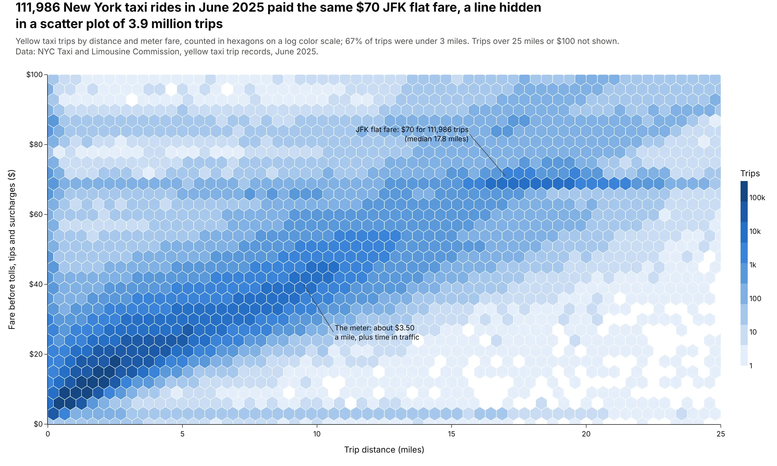
Hexbin plot of 3.9 million New York yellow taxi trips in June 2025 by distance and fare, on a log color scale. A dense diagonal band shows the metered fare rising with distance, and a separate flat band at $70 between about 15 and 25 miles shows the JFK flat fare paid on 111,986 trips

Data: NYC Taxi and Limousine Commission, yellow taxi trip records, June 2025.

How do you read a hexbin plot? In the example above, notice these things:

Each hexagon is a bin that counts the trips whose distance and fare fall inside it, so one mark stands for many trips instead of one.
Color is the number of trips, on a log scale where each labeled step on the color bar is 10 times more trips. The darkest hexagons all sit in the bottom left, among the short rides that made up most of the month's trips.
The diagonal band is the meter, which charges $0.70 per fifth of a mile plus time in slow traffic, so the fare rises with distance.
The flat band at $70 is the JFK flat fare, a single price between Manhattan and the airport whatever the distance, which a scatter plot of every trip would bury under the rest.
Watch out for the log scale when you compare colors. The hexagons lighter than the 1k mark on the color bar fill most of the chart, yet together they hold under 5% of the rides.

It's often used for charts like these:

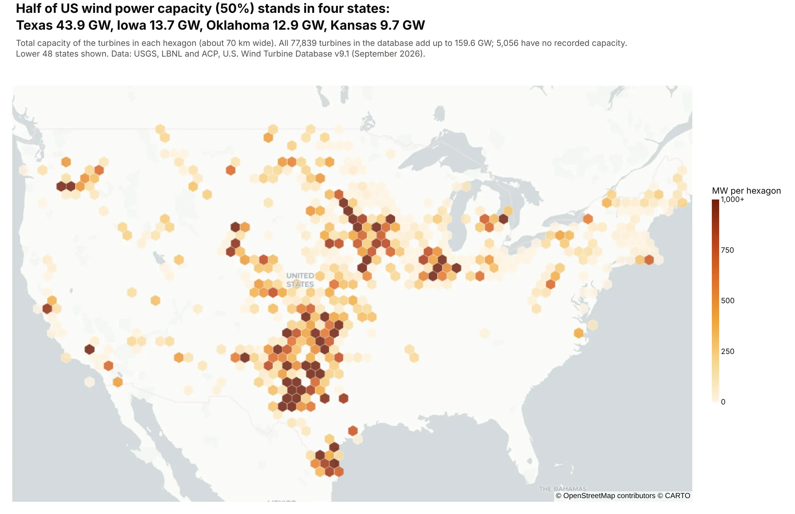
Hexbin map of the lower 48 US states in which each hexagon is colored by the total capacity of the wind turbines inside it. The darkest hexagons, over 1,000 MW each, run in a belt from west Texas through Oklahoma and Kansas to Iowa and Minnesota

Points on a map, adding up a value instead of counting them. Texas, Iowa, Oklahoma and Kansas hold 50% of the 159.6 GW of capacity in the US Wind Turbine Database. Data: USGS, LBNL and ACP, U.S. Wind Turbine Database.

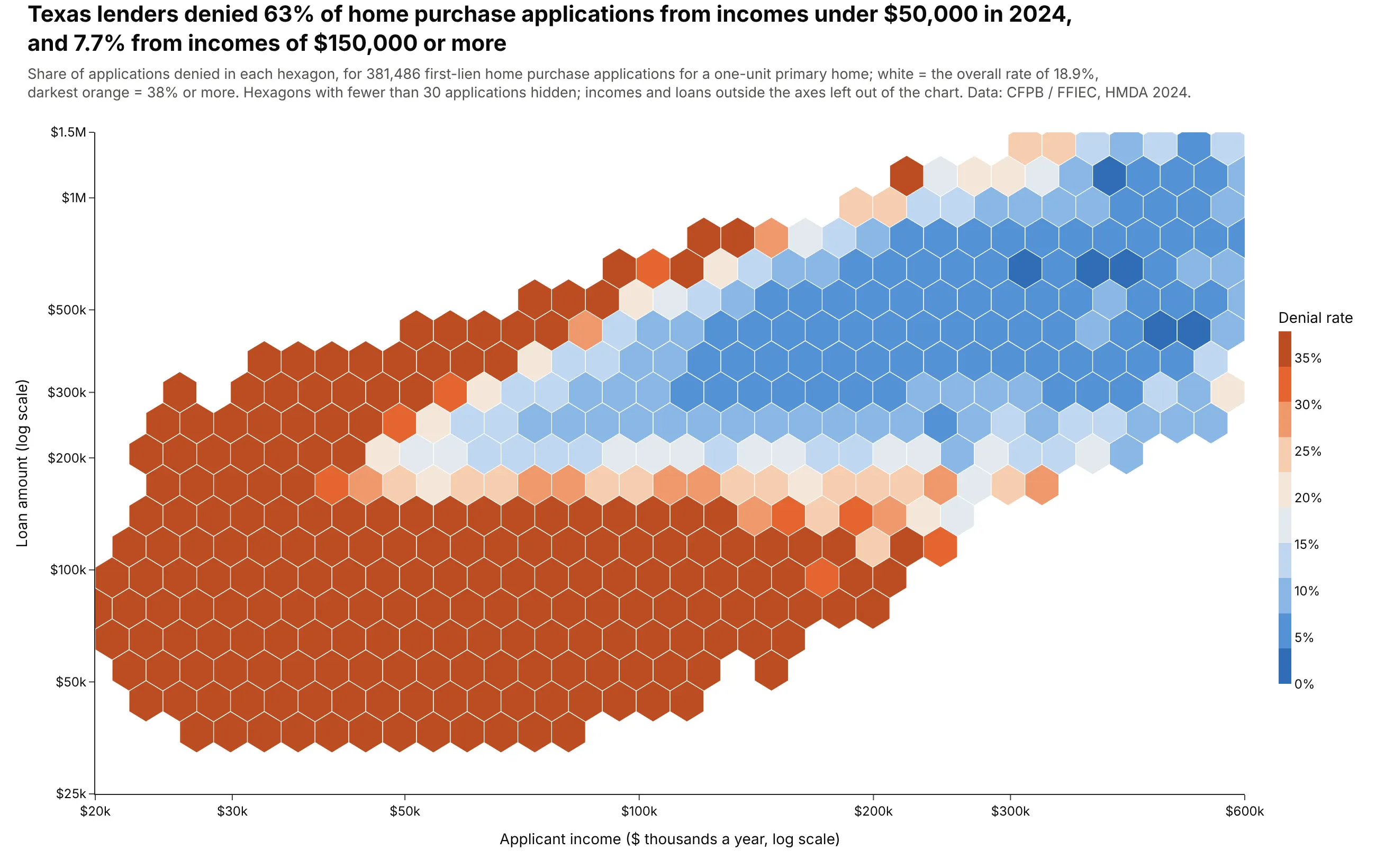
Hexbin plot of 381,486 Texas home purchase mortgage applications in 2024 by applicant income and loan amount on log axes, each hexagon colored by the share denied. Low incomes and small loans are dark orange, with denial rates over 38%, and high incomes are blue, under 10%

The rate of an outcome across two numbers. Texas lenders denied 63% of applications from incomes under $50,000 and 7.7% from incomes of $150,000 or more. Data: CFPB and FFIEC, HMDA 2024.

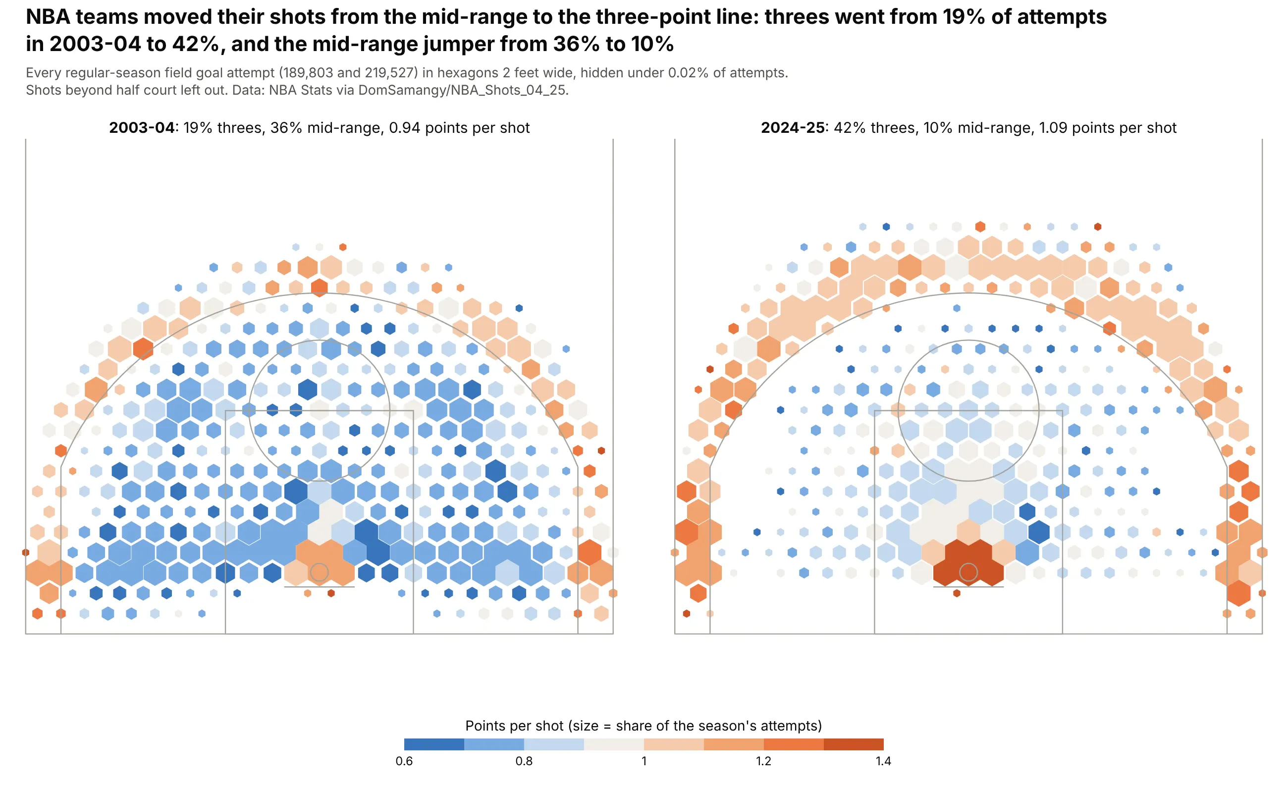
Two NBA half courts with shot charts for 2003-04 and 2024-25. Hexagon size shows how often teams shot from each spot and color shows points per shot. In 2003-04 the mid-range is covered in blue hexagons, and in 2024-25 the shots sit at the rim and in an orange band beyond the three-point line

A shot chart. Threes went from 19% of NBA attempts in 2003-04 to 42% in 2024-25, and the mid-range jumper from 36% to 10%. Data: NBA Stats via DomSamangy/NBA_Shots_04_25.

A short history

Daniel Carr and colleagues proposed hexagon binning in 1987 in "Scatterplot Matrix Techniques for Large N" (Journal of the American Statistical Association), for scatter plot matrices with too many points to draw. They chose hexagons because they are closer to circles than squares, so the bins look less like a grid and every neighbor is the same distance away. Hexagons later became a common grid for basketball shot charts and for maps, where Uber's open-source H3 index covers the globe in hexagons.

Alternatives to a hexbin plot

Here's the same set of 24,709 Paris apartment sales drawn six ways. Some are better for the question, some worse, some just different:

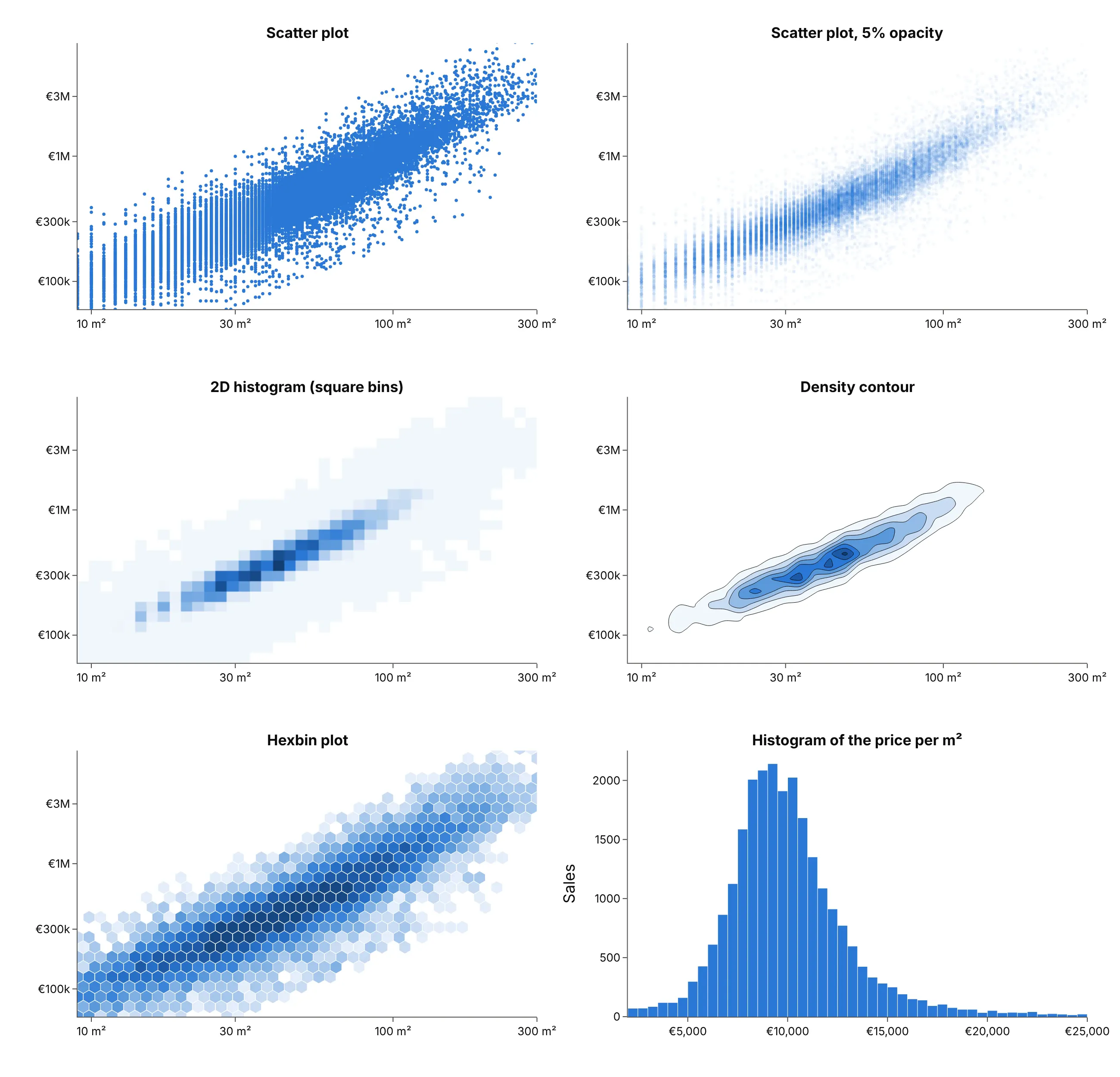
The same 24,709 Paris apartment sales in 2024 by living area and price, drawn six ways: a scatter plot that is a solid blue mass with vertical stripes at whole square meters, a scatter plot at 5% opacity, a 2D histogram with square bins, a density contour, a hexbin plot, and a histogram of the price per square meter peaking near 10,000 euros

Scatter plot (worse past about 10,000 points, better below). Every point is visible, so it shows outliers and small groups best, but here 24,709 dots overlap into a solid mass.
Transparent scatter plot (works too). Low marker.opacity shows density, but the shading isn't a number you can read off a colorbar, and it still sends every point to the browser.
2D histogram (works too). px.density_heatmap counts points in square bins and is built into Plotly, so it's the quickest option. Square bins make a visible grid, and its colors follow the counts on a linear scale, so the sparse bins disappear here. See our heatmap guide.
Density contour (different). px.density_contour smooths the counts into lines, which shows the shape well but hides individual sparse areas. See our contour plot guide.
Histogram of a ratio (better when only the ratio matters). If the question is the price per square meter, one histogram answers it directly.

How to make a hexbin plot

With AI

ChatGPT, Claude Code, GitHub Copilot, Cursor and other AI tools are excellent at writing Plotly code. Name Plotly in the prompt, say that the hexagons must look regular, and say what the color means:

Make a plotly hexbin plot from trips.csv (columns: distance_mi, fare_usd).

- Bin the points into pointy-top hexagons with numpy,
  sized so they look regular for the plot area's width and height.
- Draw all hexagons of one color class as ONE go.Scatter with fill="toself" and None
  between hexagons (about 9 classes), not one trace or shape per hexagon.
- Color by count on a log10 scale; add an invisible marker trace at the hexagon
  centers for the hover text and the colorbar.
- Axis ranges 0-25 miles and $0-100; say in the subtitle what is left out.
- A title that states the main takeaway, with the source in a muted subtitle.
- Save it as hexbin.html and as a PNG at 2x scale.

With Plotly Studio

Plotly Studio is a desktop app where you point an AI at a dataset and it builds charts and a Dash app around your questions. Ask for a hexbin plot the same way:

Show a hexbin plot of trip distance against fare with a log color scale for the count of trips, and add a dropdown to switch between the hours of the day.

Make a hexbin plot in Python or JavaScript

This is the code AI tools write under the hood. You can make a hexbin plot with Plotly by binning the points with numpy and drawing each color class as one filled go.Scatter, with hexagons separated by None. An invisible marker trace at the hexagon centers carries the hover text and the colorbar. Every example below builds on the same idea:

import numpy as np
import pandas as pd
import plotly.graph_objects as go
from plotly.colors import sample_colorscale


def make_hexbin(x, y, nx=40, aspect=0.6, n_colors=8, colorscale="Blues", log_color=True):
    """Bin x, y into regular hexagons (on a plot area of height/width = aspect) and draw them."""
    x, y = np.asarray(x, float), np.asarray(y, float)
    x0, y0 = x.min(), y.min()
    w = (x.max() - x0) / nx                                 # hexagon width in x units
    h = np.sqrt(3) / 2 * (y.max() - y0) / (nx * aspect)     # row spacing in y units
    u, v = (x - x0) / w, (y - y0) / h
    ua, va = np.round(u), 2 * np.round(v / 2)               # two offset grids of centers;
    ub, vb = np.floor(u) + 0.5, 2 * np.floor(v / 2) + 1     # each point takes the nearer one
    a = (u - ua) ** 2 + 0.75 * (v - va) ** 2 <= (u - ub) ** 2 + 0.75 * (v - vb) ** 2
    hexes = pd.DataFrame({"u": np.where(a, ua, ub), "v": np.where(a, va, vb)}).value_counts().reset_index()
    z = np.log10(hexes["count"]) if log_color else hexes["count"]
    k = np.minimum((z - z.min()) / (z.max() - z.min() + 1e-9) * n_colors, n_colors - 1).astype(int)
    colors = sample_colorscale(colorscale, list((np.arange(n_colors) + 0.5) / n_colors))
    ang = np.radians(90 + 60 * np.arange(7))
    fig = go.Figure()
    for i, color in enumerate(colors):                     # one filled trace per color class
        xs, ys = [], []
        for u_, v_ in hexes.loc[k == i, ["u", "v"]].itertuples(index=False):
            xs += list(x0 + (u_ + np.cos(ang) / np.sqrt(3)) * w) + [None]
            ys += list(y0 + (v_ + 2 / 3 * np.sin(ang)) * h) + [None]
        fig.add_scatter(x=xs, y=ys, fill="toself", mode="lines", fillcolor=color,
                        line=dict(color="white", width=0.5), hoverinfo="skip", showlegend=False)
    fig.add_scatter(x=x0 + hexes.u * w, y=y0 + hexes.v * h, mode="markers", showlegend=False,
                    customdata=hexes["count"], hovertemplate="%{customdata:,} points<extra></extra>",
                    marker=dict(opacity=0, color=z, colorscale=colorscale, showscale=True))
    return fig


rng = np.random.default_rng(0)
x = rng.normal(size=200_000)
y = 0.6 * x + rng.normal(size=200_000)
make_hexbin(x, y, nx=40).show()

The examples use a fuller version of the helper that also colors by the mean of a third column, takes pre-counted rows as weights, bins on log axes and shrinks sparse hexagons for shot charts.

On a map, Plotly has it built in. create_hexbin_map draws the hexagons as a go.Choroplethmap on a tile map and can add up or average a column instead of counting:

import numpy as np
import plotly.figure_factory as ff

fig = ff.create_hexbin_map(
    data_frame=turbines, lat="lat", lon="lon", color="capacity_mw", agg_func=np.sum,
    nx_hexagon=70, opacity=0.85, min_count=1, map_style="carto-positron",
)
fig.show()

In JavaScript, plotly.js takes the same approach: count points per hexagon, then draw one filled scatter trace per shade:

<div id="chart"></div>
<script src="https://cdn.plot.ly/plotly-4.1.1.min.js"></script>
<script>
  const x = [], y = [];                              // replace with your own data
  for (let i = 0; i < 20000; i++) {
    const a = Math.random() + Math.random() + Math.random() - 1.5;
    x.push(a); y.push(0.6 * a + Math.random() - 0.5);
  }
  const nx = 30, aspect = 0.6;                       // hexagon columns, plot height / width
  const x0 = Math.min(...x), y0 = Math.min(...y);
  const w = (Math.max(...x) - x0) / nx;
  const h = Math.sqrt(3) / 2 * (Math.max(...y) - y0) / (nx * aspect);
  const counts = new Map();
  x.forEach((xi, i) => {
    const u = (xi - x0) / w, v = (y[i] - y0) / h;
    const ua = Math.round(u), va = 2 * Math.round(v / 2);
    const ub = Math.floor(u) + 0.5, vb = 2 * Math.floor(v / 2) + 1;
    const nearA = (u - ua) ** 2 + 0.75 * (v - va) ** 2 <= (u - ub) ** 2 + 0.75 * (v - vb) ** 2;
    const key = nearA ? `${ua},${va}` : `${ub},${vb}`;
    counts.set(key, (counts.get(key) || 0) + 1);
  });
  const max = Math.max(...counts.values());
  const shades = ["#c9dcf3", "#93bce8", "#5a98da", "#2a78d6", "#1d5aa6", "#123d73"];
  const traces = shades.map(c => ({type: "scatter", mode: "lines", fill: "toself", fillcolor: c,
    line: {color: "white", width: 0.5}, x: [], y: [], hoverinfo: "skip", showlegend: false}));
  for (const [key, n] of counts) {
    const [cu, cv] = key.split(",").map(Number);
    const t = traces[Math.min(shades.length - 1, Math.floor(n / max * shades.length))];
    for (let k = 0; k <= 6; k++) {
      const ang = (90 + 60 * k) * Math.PI / 180;
      t.x.push(x0 + (cu + Math.cos(ang) / Math.sqrt(3)) * w);
      t.y.push(y0 + (cv + 2 / 3 * Math.sin(ang)) * h);
    }
    t.x.push(null); t.y.push(null);
  }
  Plotly.newPlot("chart", traces);
</script>

The aspect value must match the plot area's height divided by its width, or the hexagons come out stretched.

Share it

Every Plotly chart has a Share chart button (the cloud icon in its toolbar) that uploads it to Plotly Cloud and gives you a link. Only you can see it until you change its visibility.

For a live app, put the chart in a Dash app and publish it with the Plotly Cloud CLI. Coding agents can run these commands for you:

pip install "dash[cloud]"
plotly user login
plotly app publish

If your data has to stay in your own cloud or data center, publish to Dash Enterprise instead.

Dos and don'ts

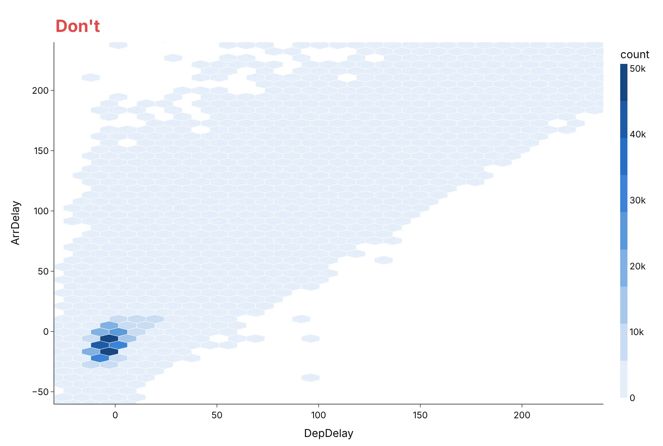
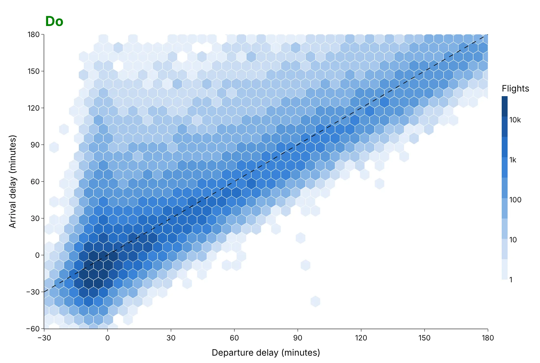
Most hexbin mistakes come from the color scale and the shape of the hexagons. Here are 599,472 US flights in June 2025 by departure and arrival delay, drawn both ways.

Don't use a linear color scale for counts that span four orders of magnitude, stretch the hexagons, let a few extreme flights set the axis range, or keep the raw column names:

A hexbin plot of flight delays with a linear color scale where one small cluster near zero is dark and everything else is the same pale blue, flattened hexagons, an axis running to 240 minutes and axis labels DepDelay and ArrDelay

Do use a log color scale, regular hexagons, a range that holds the bulk of the flights, labeled axes and a reference line where arrival delay equals departure delay:

The same flights with a log color scale from 1 to over 10,000 flights, regular hexagons, axes from -30 to 180 minutes labeled Departure delay and Arrival delay, and a dashed diagonal line

Pick the hexagon size

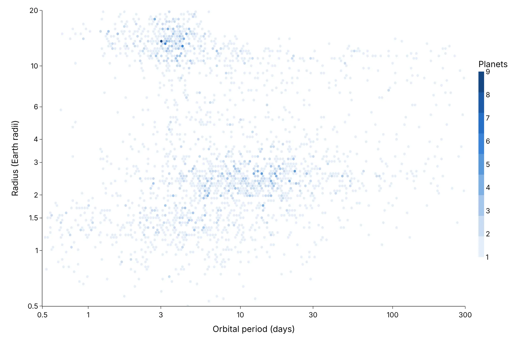
The number of hexagon columns (nx) is the main decision, like the bin width of a histogram. Here are three choices for the same 2,633 exoplanets.

Too big (14 columns). The two groups of small planets merge, and the gap between them is gone.

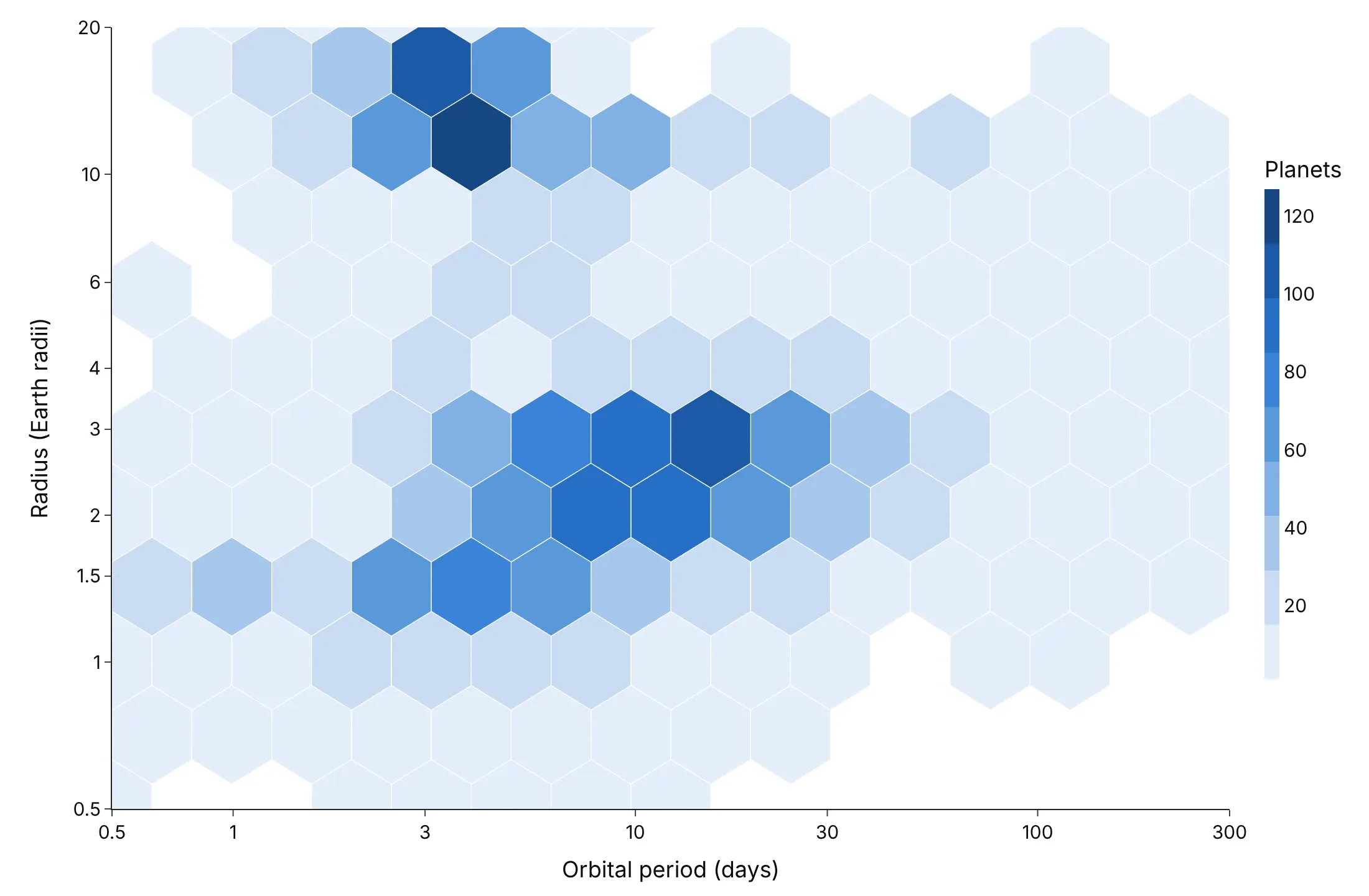
Hexbin plot of exoplanets by orbital period and radius with 14 large hexagons across, where super-Earths and sub-Neptunes merge into one blob

About right (55 columns). The super-Earths and sub-Neptunes separate, with a band of fewer planets near 1.8 Earth radii between them.

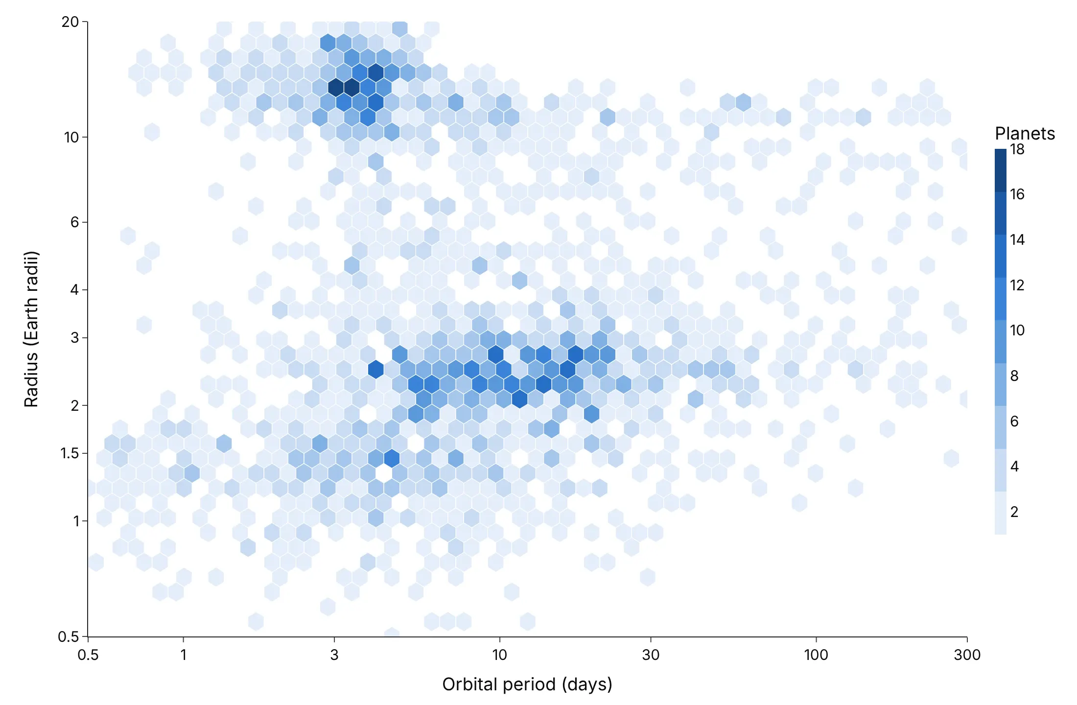
The same exoplanets with 55 hexagons across, showing a cluster of hot Jupiters at the top, and super-Earths below 1.6 Earth radii separated from sub-Neptunes above 2 Earth radii

Too small (160 columns). Most hexagons hold one or two planets, so it reads as a scatter plot again.

The same exoplanets with 160 tiny hexagons across, most holding one or two planets, which looks like a faint scatter plot

Checklist

Write a title that states the takeaway.
Use a log color scale when counts span more than two orders of magnitude.
Keep the hexagons regular: match the binning's aspect ratio to the plot area, or fix the axis scales.
Say in the subtitle what's left out (points beyond the axes, hexagons below a minimum count).
Color by a mean or a rate only where each hexagon holds enough points (mincnt, often 20-30).

Don't

Use a hexbin for a few hundred points, where a scatter plot shows more.
Use a rainbow color scale, which creates edges that aren't in the data.
Bin whole-number data with hexagons that don't line up with the values (example 5).

Options to customize

These are the settings that matter for a hexbin built from go.Scatter, and for create_hexbin_map. The full lists are in the Plotly scatter reference and the hexbin map documentation.

nx (the helper): hexagon columns across the x range; 30-60 for most charts.
aspect (the helper): the plot area's height divided by its width, so hexagons come out regular.
go.Scatter(fill="toself") with None between hexagons: draws one color class of hexagons as one trace.
fillcolor: the color of each class; take it from plotly.colors.sample_colorscale.
line.color, line.width: white 0.5-1 px borders separate the hexagons; set width 0 for a smooth look.
marker.colorscale, cmin, cmax on the invisible center trace: the colorbar and its range.
hovertemplate, customdata: the count or the mean in each hexagon on hover.
xaxis.type="log", yaxis.type="log": bin in log10 space, then draw on log axes (examples 4 and 8).
yaxis.scaleanchor="x": equal scales, for courts, maps in feet or minutes against minutes.
agg_func (create_hexbin_map): np.sum, np.mean or np.median of the color column instead of a count.
nx_hexagon, min_count (create_hexbin_map): hexagon columns and the minimum points to draw one.
map_style, opacity, center, zoom (create_hexbin_map): the base map and the view.
px.density_heatmap(nbinsx=, nbinsy=, histfunc=): the built-in square-bin alternative.

More hexbin plot examples

Nine more hexbin plots built from real public data, each with its source, the technique that makes it work and a prompt to rebuild it.

1. Wind and solar against demand on the Texas grid

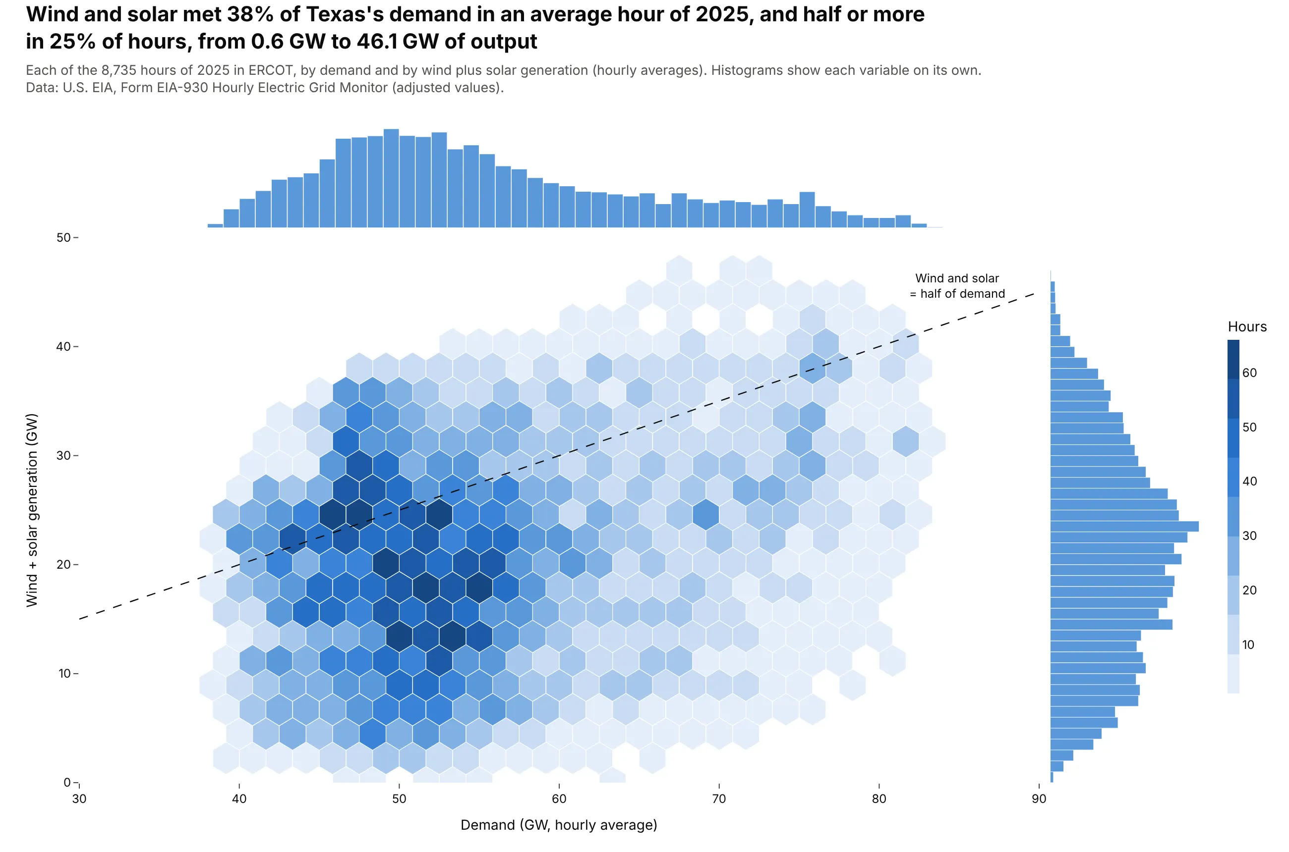
Hexbin plot of the 8,735 hours of 2025 on the ERCOT grid by demand and by wind plus solar generation, with histograms of each on the top and right. Most hours sit between 45 and 55 GW of demand and 10 to 30 GW of wind and solar, and a dashed line marks where wind and solar equal half of demand

Wind and solar met 38% of Texas's demand in an average hour of 2025, and half or more in 25% of hours. Output ranged from 0.6 GW to 46.1 GW, at any level of demand. Data: U.S. EIA, Form EIA-930 Hourly Electric Grid Monitor, ERCOT, 2025.

Tip: add the hexbin traces to the main cell of a 2x2 make_subplots grid with shared axes, and put a histogram of each variable in the cells above and to the right.

Get the data from the U.S. EIA Hourly Electric Grid Monitor (Form EIA-930), six-month BALANCE files
for 2025 (eia.gov/electricity/gridmonitor), balancing authority ERCO, adjusted values
(columns: date, hour, demand_mw, wind_mw, solar_mw).

Make a plotly hexbin plot of demand (GW) on x against wind + solar (GW) on y.
- Bin into regular hexagons (about 36 columns), one filled go.Scatter per color class.
- Use make_subplots(2, 2) with shared axes: hexbin bottom left, a histogram of demand on top,
  a horizontal histogram of wind + solar on the right.
- Add a dashed line where wind + solar = half of demand.
- Title with the average share of demand met by wind and solar.

2. Stock returns against trading volume

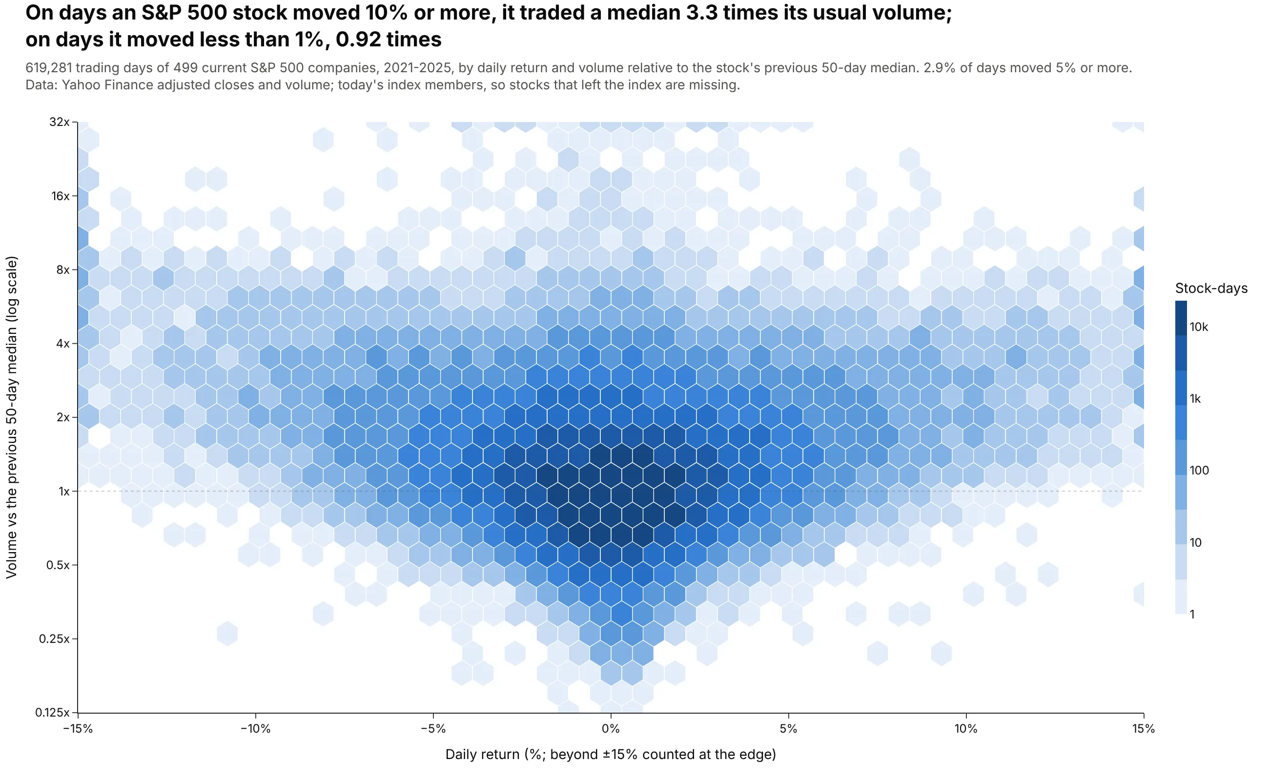
Hexbin plot of 619,281 daily observations of 499 S&P 500 stocks from 2021 to 2025 by daily return and volume relative to the previous 50-day median, on a log color scale. The densest hexagons sit near 0% and 1x volume, and the cloud widens into a V shape, with large moves in either direction at two to eight times normal volume

On days an S&P 500 stock moved 10% or more, it traded a median 3.3 times its usual volume, against 0.92 times on days it moved less than 1%. The 619,281 stock-days form a V, because big moves in either direction come with heavy trading. Data: Yahoo Finance daily prices and volume for current S&P 500 members, 2021-2025.

Tip: for big data, count the points on a fine grid in pandas first and pass the counts as weights to the hexbin, which keeps the CSV at 171 KB instead of 600,000 rows.

Get the data from Yahoo Finance: daily adjusted closes and volume for every current S&P 500
company (list from github.com/datasets/s-and-p-500-companies), 2021-2025
(columns: ticker, date, return_pct, rel_volume = volume / median volume of the previous 50 days).

Make a plotly hexbin plot of return_pct (x, clipped to +/-15%) against log2(rel_volume) (y).
- Pre-aggregate: count stock-days on a 0.1-point x 0.05 grid, then hexbin with those counts as weights.
- Log10 color scale for the counts; y ticks labeled 0.25x, 0.5x, 1x, 2x ... 32x.
- Title with the median relative volume on days with |return| >= 10% vs < 1%.

3. A century of oil and gas drilling in Kansas

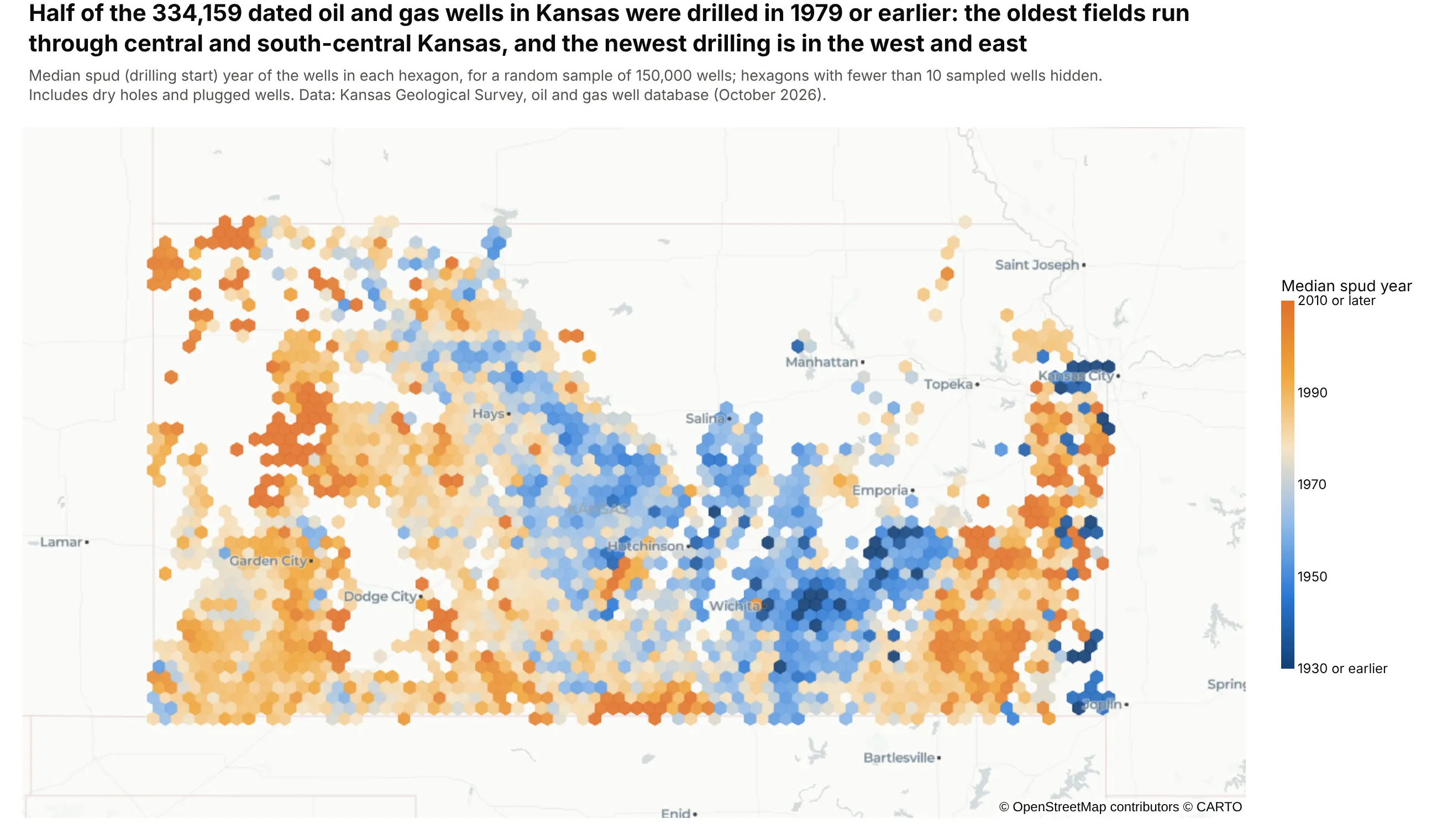
Hexbin map of Kansas in which each hexagon is colored by the median year its oil and gas wells were drilled, from dark blue for 1930 or earlier to orange for 2010 or later. The oldest hexagons run through central and south-central Kansas around Wichita and El Dorado, and the newest are in western and eastern Kansas

Half of the 334,159 dated oil and gas wells in Kansas were drilled in 1979 or earlier. Colored by the median drilling year, the map shows the oldest fields in central and south-central Kansas and newer drilling in the west and east. Data: Kansas Geological Survey, oil and gas well database (a random sample of 150,000 wells is drawn).

Tip: create_hexbin_map(..., color="spud_year", agg_func=np.median, min_count=10) colors each hexagon by a summary of a third column and hides hexagons with too few wells for a median.

Get the data from the Kansas Geological Survey oil and gas well database, full download ks_wells.zip
(kgs.ku.edu/PRS/Ora_Archive/ks_wells.zip)
(columns: LATITUDE, LONGITUDE, SPUD as DD-MON-YYYY, STATUS).

Make a plotly hexbin map with plotly.figure_factory.create_hexbin_map.
- color = spud year, agg_func = np.median, nx_hexagon = 80, min_count = 10.
- Diverging scale from dark blue (1930 or earlier) to orange (2010 or later), range 1930-2010.
- carto-positron map style, zoomed to Kansas, no hexagon borders.
- Title with the median drilling year of all wells; note any sampling in the subtitle.

4. What a Paris apartment cost in 2024

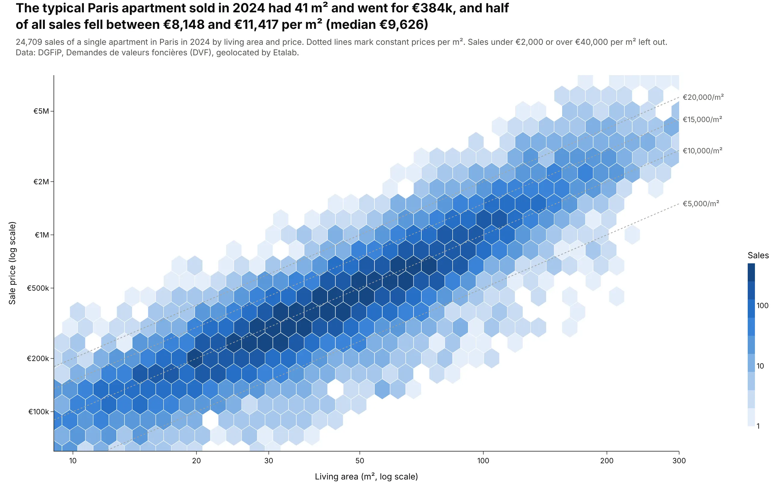
Hexbin plot of 24,709 Paris apartment sales in 2024 by living area and price on log axes, with dotted lines at 5,000, 10,000, 15,000 and 20,000 euros per square meter. The densest hexagons follow the 10,000 euro line from about 20 to 70 square meters

The typical Paris apartment sold in 2024 had 41 m² and went for €384,000, and half of all sales fell between €8,148 and €11,417 per m². On log-log axes, constant prices per m² are straight lines, so readers can read the ratio off the chart. Data: DGFiP, Demandes de valeurs foncières (DVF), geolocated by Etalab.

Tip: bin in log10 space and draw the hexagons on log axes, so they stay regular on screen.

Get the data from France's DVF open data, geolocated by Etalab, Paris 2024
(files.data.gouv.fr/geo-dvf/latest/csv/2024/departements/75.csv.gz); keep sales of exactly one
apartment (columns: id_mutation, surface_reelle_bati, valeur_fonciere).

Make a plotly hexbin plot of living area (x) against price (y), both on log axes.
- Bin log10 values into regular hexagons and draw them on log axes; log10 color for counts.
- Leave out sales under 2,000 or over 40,000 euros per m2 and say so.
- Dotted gray lines at 5,000, 10,000, 15,000 and 20,000 euros per m2, labeled at the right edge.
- Title with the median size, price and price per m2.

5. Blood pressure by age

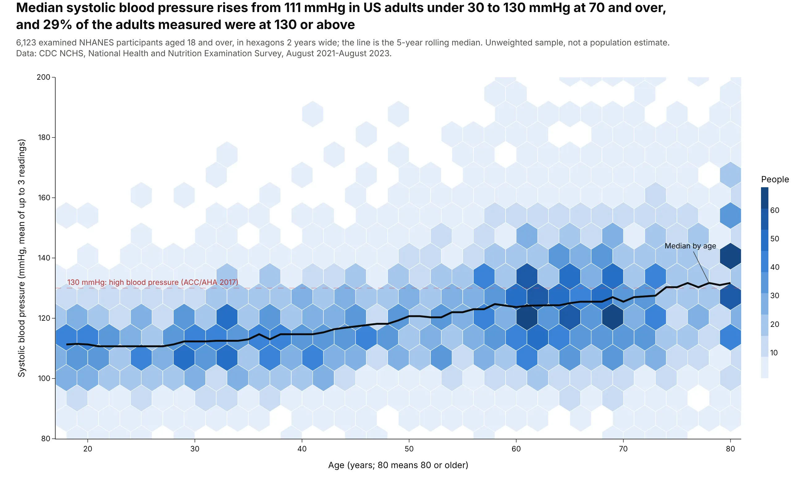
Hexbin plot of 6,123 US adults from NHANES 2021-2023 by age and systolic blood pressure, in hexagons 2 years wide, with a black median line rising from 111 mmHg under 30 to about 130 at 70 and over, and a dashed red line at 130 mmHg

Median systolic blood pressure rises from 111 mmHg in US adults under 30 to 130 mmHg at 70 and over, and 29% of the 6,123 adults measured were at 130 or above. The line on top is the 5-year rolling median. Data: CDC NCHS, National Health and Nutrition Examination Survey, August 2021-August 2023 (unweighted).

Tip: ages are whole numbers, so make the hexagons exactly 2 years wide and start the x range at an odd age, which puts every hexagon center on a whole year instead of leaving striped empty columns.

Get the data from CDC NHANES 2021-2023 (wwwn.cdc.gov/Nchs/Data/Nhanes/Public/2021/DataFiles/),
DEMO_L.xpt and BPXO_L.xpt joined on SEQN; adults 18+; systolic = mean of BPXOSY1-3
(columns: age, sex, systolic, diastolic).

Make a plotly hexbin plot of age (x, 17-81) against systolic blood pressure (y, 80-200).
- Hexagons exactly 2 years wide (32 columns) so centers fall on whole ages.
- Overlay a black line of the 5-year rolling median by age.
- A dashed red line at 130 mmHg labeled as the 2017 ACC/AHA threshold.
- Note that age 80 means 80 or older and that the sample is unweighted.

6. Approved drugs against Lipinski's rule of five

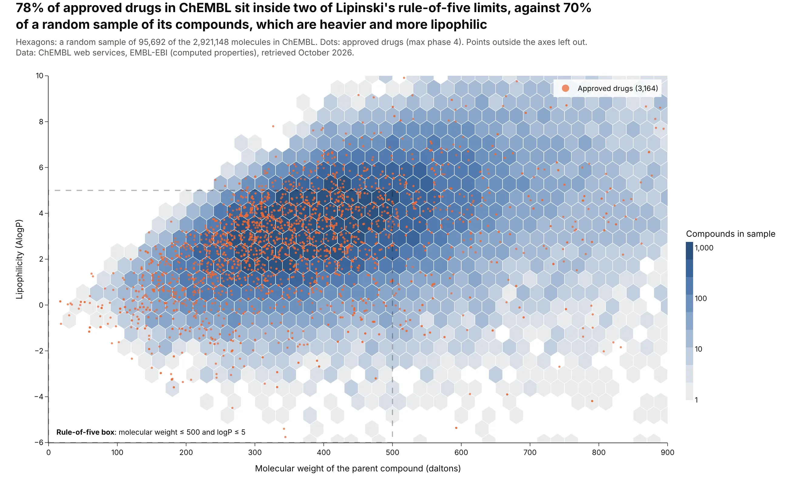
Hexbin plot of a random sample of 95,692 ChEMBL compounds by molecular weight and AlogP, with 3,164 approved drugs drawn as small orange dots on top and a dashed box for molecular weight 500 or less and logP 5 or less. Most drugs sit inside the box

78% of the 3,164 approved drugs in ChEMBL sit inside two of Lipinski's rule-of-five limits, against 70% of a random sample of its compounds, which are heavier (median 400 against 345 daltons) and more lipophilic. Data: ChEMBL web services, EMBL-EBI (Zdrazil et al., 2023).

Tip: draw the background population as gray-blue hexagons and the small group you care about as orange dots on top, so the dots stay visible.

Get the data from the ChEMBL web services (ebi.ac.uk/chembl/api/data/molecule.json): a random sample
of about 100,000 molecules and every molecule with max_phase = 4
(columns: chembl_id, mw = mw_freebase, alogp, max_phase).

Make a plotly hexbin plot of molecular weight (x, 0-900) against AlogP (y, -6 to 10) for the sample.
- Gray-blue sequential scale, log10 color for counts.
- Approved drugs as 3.5 px orange dots on top, with a legend entry.
- A dashed, unfilled box for MW <= 500 and logP <= 5, labeled.
- Title with the share of drugs and of the sample inside the box.

7. A year of aftershocks after the Ridgecrest earthquake

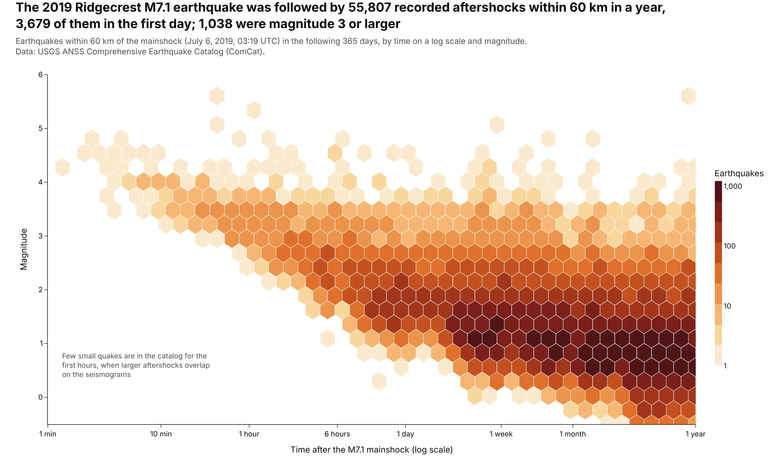
Hexbin plot of 55,807 earthquakes in the year after the 2019 Ridgecrest M7.1 mainshock by time on a log scale from 1 minute to 1 year and magnitude, on a log color scale. In the first hour only quakes above about magnitude 3 are recorded, and the smallest recorded magnitude falls toward 0 over the following weeks

The 2019 Ridgecrest M7.1 earthquake was followed by 55,807 recorded aftershocks within 60 km in a year, 3,679 of them in the first day. The log time axis shows the catalog filling in: in the first hour, 95% of recorded quakes were above magnitude 2.98, and after 100 days above magnitude -0.02. Data: USGS ANSS Comprehensive Earthquake Catalog (ComCat).

Tip: bin time in log10 space (log_x=True in the helper), because aftershock rates fall by orders of magnitude.

Get the data from the USGS earthquake catalog API (earthquake.usgs.gov/fdsnws/event/1/query),
CSV, within 60 km of 35.77 N, 117.60 W, from 2019-07-04 to one year after the M7.1 mainshock at
2019-07-06 03:19:53 UTC, in 5-day windows (columns: time, magnitude, depth_km).

Make a plotly hexbin plot of time after the mainshock (x, log scale, 1 minute to 1 year)
against magnitude (y).
- Bin log10(days) into regular hexagons; log10 color for counts.
- X ticks labeled 1 min, 10 min, 1 hour, 6 hours, 1 day, 1 week, 1 month, 1 year.
- Title with the number of aftershocks, the first-day count and the count of M3+.

8. The radius valley between super-Earths and sub-Neptunes

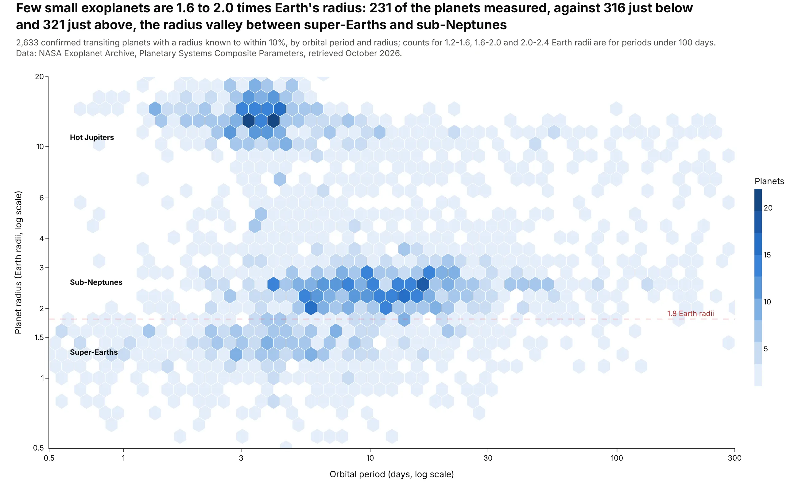
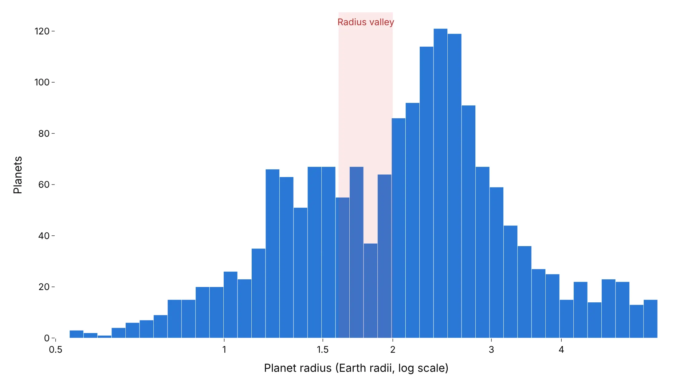
Hexbin plot of 2,633 transiting exoplanets with well-measured radii by orbital period and radius on log axes. Hot Jupiters cluster near 3 days and 13 Earth radii, and below them super-Earths and sub-Neptunes form two bands with fewer planets near a dashed line at 1.8 Earth radii

Few small exoplanets are 1.6 to 2.0 times Earth's radius: 231 of the planets measured, against 316 just below and 321 just above. Fulton et al. (2017) called this gap the radius valley. Data: NASA Exoplanet Archive, Planetary Systems Composite Parameters (transiting planets with radii known to within 10%).

Tip: keep only planets with precise radii, because measurement error fills a narrow gap with planets from both sides.

Get the data from the NASA Exoplanet Archive TAP service, table pscomppars
(exoplanetarchive.ipac.caltech.edu/TAP/sync)
(columns: pl_name, discoverymethod, pl_orbper, pl_rade, pl_radeerr1, pl_radeerr2).

Make a plotly hexbin plot of orbital period (x, 0.5-300 days) against radius (y, 0.5-20 Earth
radii), both on log axes, for transiting planets with radius uncertainty <= 10%.
- About 55 hexagon columns; linear color for counts.
- A dashed line at 1.8 Earth radii; label hot Jupiters, sub-Neptunes and super-Earths.
- Title with the counts at 1.2-1.6, 1.6-2.0 and 2.0-2.4 Earth radii for periods under 100 days.

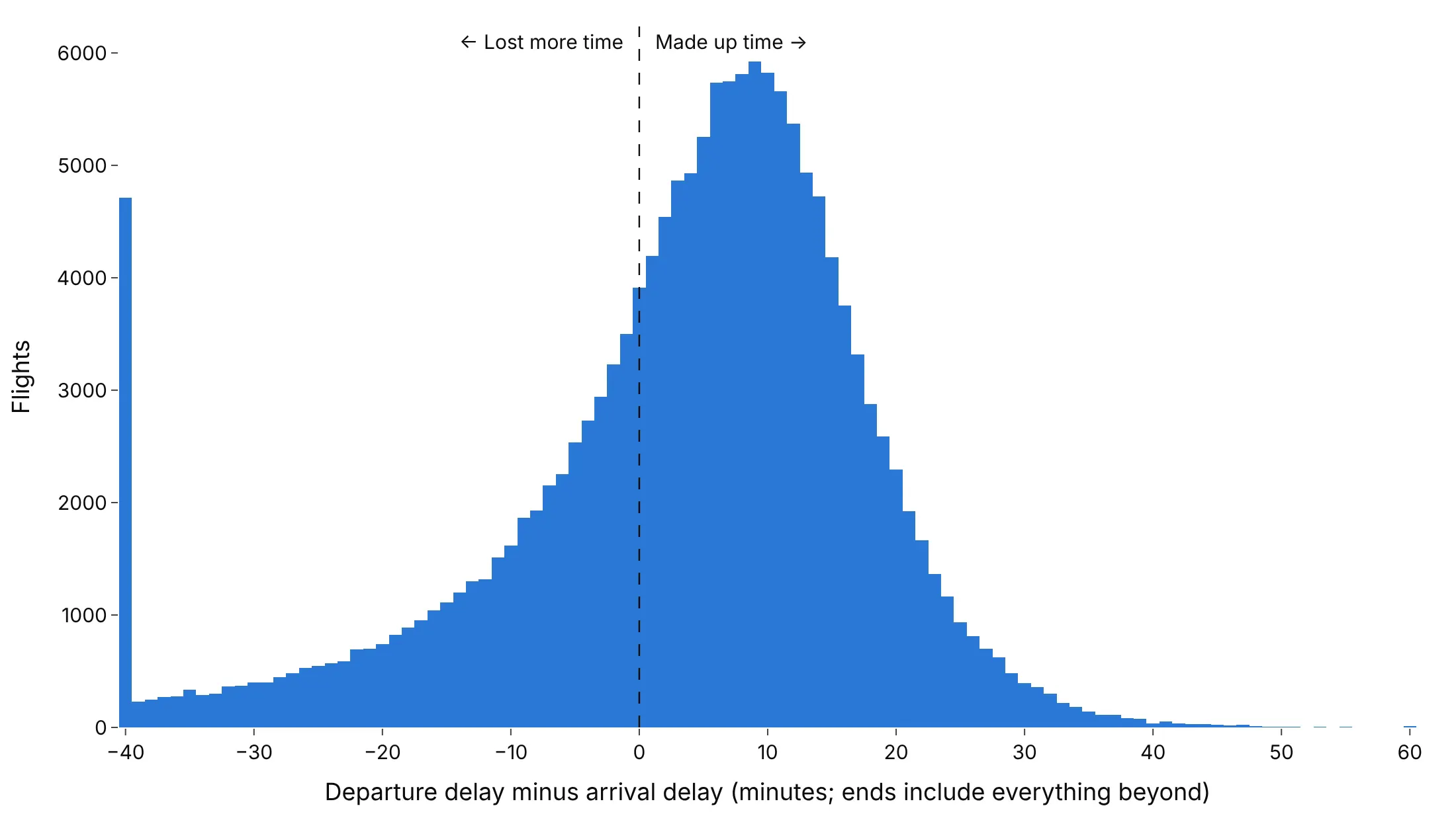
Another way to see it: a histogram of the radius alone shows the valley as a dip between 1.6 and 2.0 Earth radii, but loses the orbital period, which tells hot Jupiters apart from the small planets.

Histogram of the radii of transiting planets with periods under 100 days on a log scale, with a dip between 1.6 and 2.0 Earth radii shaded and labeled radius valley, between a group near 1.3 and a taller peak near 2.5

9. Late flights rarely make up the time

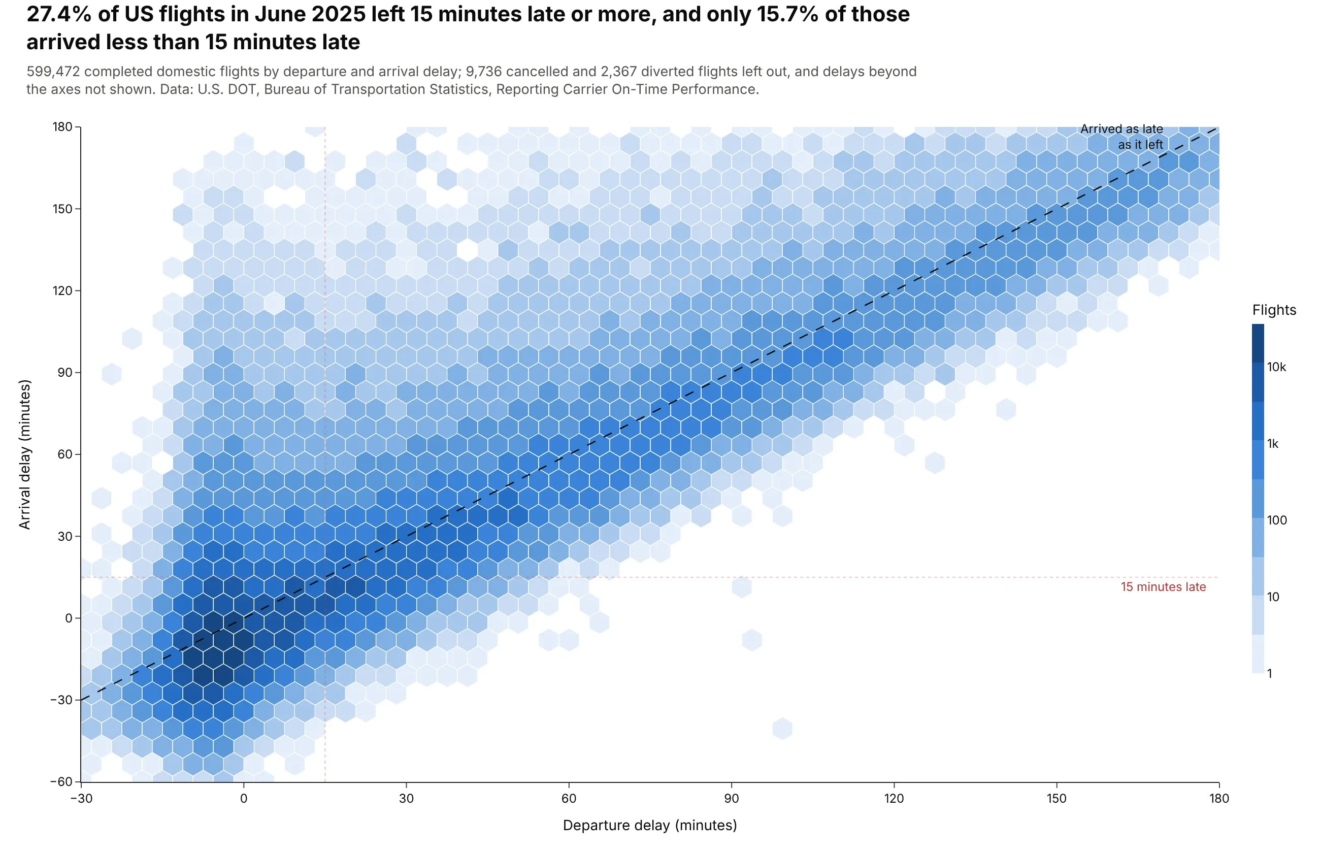
Hexbin plot of 599,472 US domestic flights in June 2025 by departure delay and arrival delay on a log color scale, with a dashed diagonal where arrival delay equals departure delay. The flights hug the diagonal, slightly below it, and the densest hexagons are near 0 minutes

27.4% of US flights in June 2025 left 15 minutes late or more, and only 15.7% of those arrived less than 15 minutes late. The hexagons hug the diagonal: a late departure almost always means a late arrival. Data: U.S. DOT, Bureau of Transportation Statistics, Reporting Carrier On-Time Performance, June 2025.

Tip: a dashed y = x line turns the chart into a before-and-after comparison, with flights below it making up time in the air.

Get the data from the BTS Reporting Carrier On-Time Performance file for June 2025
(transtats.bts.gov/PREZIP/On_Time_Reporting_Carrier_On_Time_Performance_1987_present_2025_6.zip)
(columns: DepDelay, ArrDelay, Cancelled, Diverted).

Make a plotly hexbin plot of departure delay (x, -30 to 180 min) against arrival delay (y, -60 to 180).
- Count flights on a 1-minute grid first, then hexbin with the counts as weights.
- Log10 color for counts; a dashed y = x line; dotted lines at 15 minutes on both axes.
- Title with the share of flights 15+ minutes late and the share of those that arrived < 15 min late.

Another way to see it: a histogram of departure delay minus arrival delay, for the flights that left 15 minutes late or more, shows that 67% made up some time in the air, but usually only a few minutes.

Histogram of departure delay minus arrival delay for US flights that left 15 or more minutes late in June 2025, peaking near 8 minutes made up, with a long tail of flights that lost more time