Scatter Plot Matrices - A Complete Guide

TL;DR

• A scatter plot matrix draws a scatter plot for every pair of variables in a grid, one row and one column per variable, so you see every pairwise relationship in a table of 3 to 8 numeric columns at once.
• Scatter plot matrices are also known as scatterplot matrices, pair plots and SPLOMs, and are similar to parallel coordinates plots and correlation heatmaps.
• Use one as the first look at a new table, before a model, or to see which measures separate your groups. Past about 8 variables the panels get too small, so use a correlation heatmap instead.
• Its best feature is linked brushing: select points in one panel and the same records light up in every other panel.
• Any coding agent can make one with Plotly in a minute. In Python it's px.scatter_matrix(df, dimensions=[...], color=...), drawn with WebGL so tens of thousands of points stay interactive.

What is a scatter plot matrix?

Scatter plot matrices look like this:

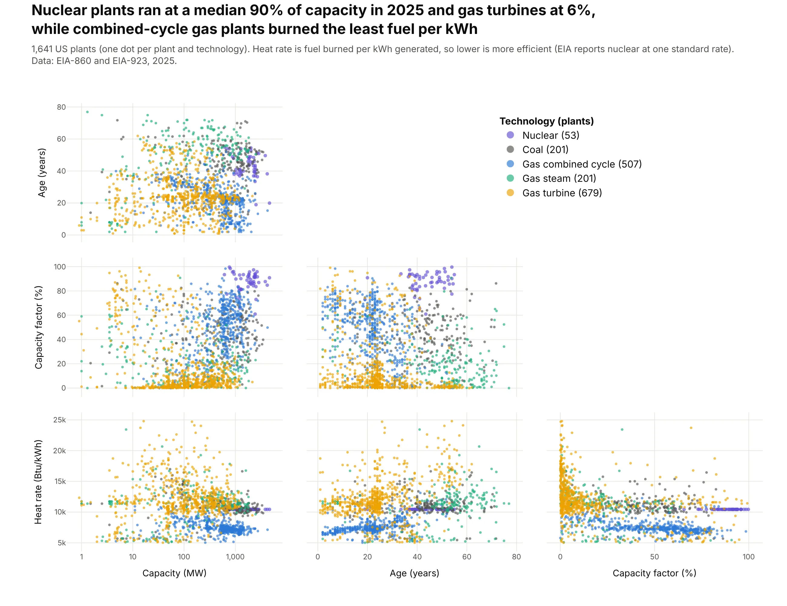
Data: EIA-860 and EIA-923, 2025 final data.

How do you read a scatter plot matrix? In the example above, notice these things:

• Each dot is one power plant, and the same 1,641 dots appear in every panel, colored by technology, with purple for nuclear and yellow for gas turbines.
• Each panel plots one pair of the four measures, with the row giving the y axis and the column the x axis, so the panel in the capacity factor row and the age column puts each plant's age against how hard it ran. The upper half would only repeat these panels with the axes swapped, so it holds the legend instead.
• Follow one color from panel to panel to see a group from every angle. The purple nuclear plants sit in a tight cluster near the top of the capacity factor row, while the yellow gas turbines pile up along its 0 line, because most of them ran at less than a tenth of their capacity over the year.
• In the heat rate row, the blue combined-cycle plants form a band below the other technologies, because they burn the least fuel for each kWh they generate (a median of 7,328 Btu/kWh, the lowest of the five groups).
• Watch the axes before you compare panels. Capacity is on a log scale, so each gridline is 10 times the one before, and the flat purple line in the heat rate row is an almost constant standard rate that EIA reports for nuclear plants.

It's often used for charts like these:

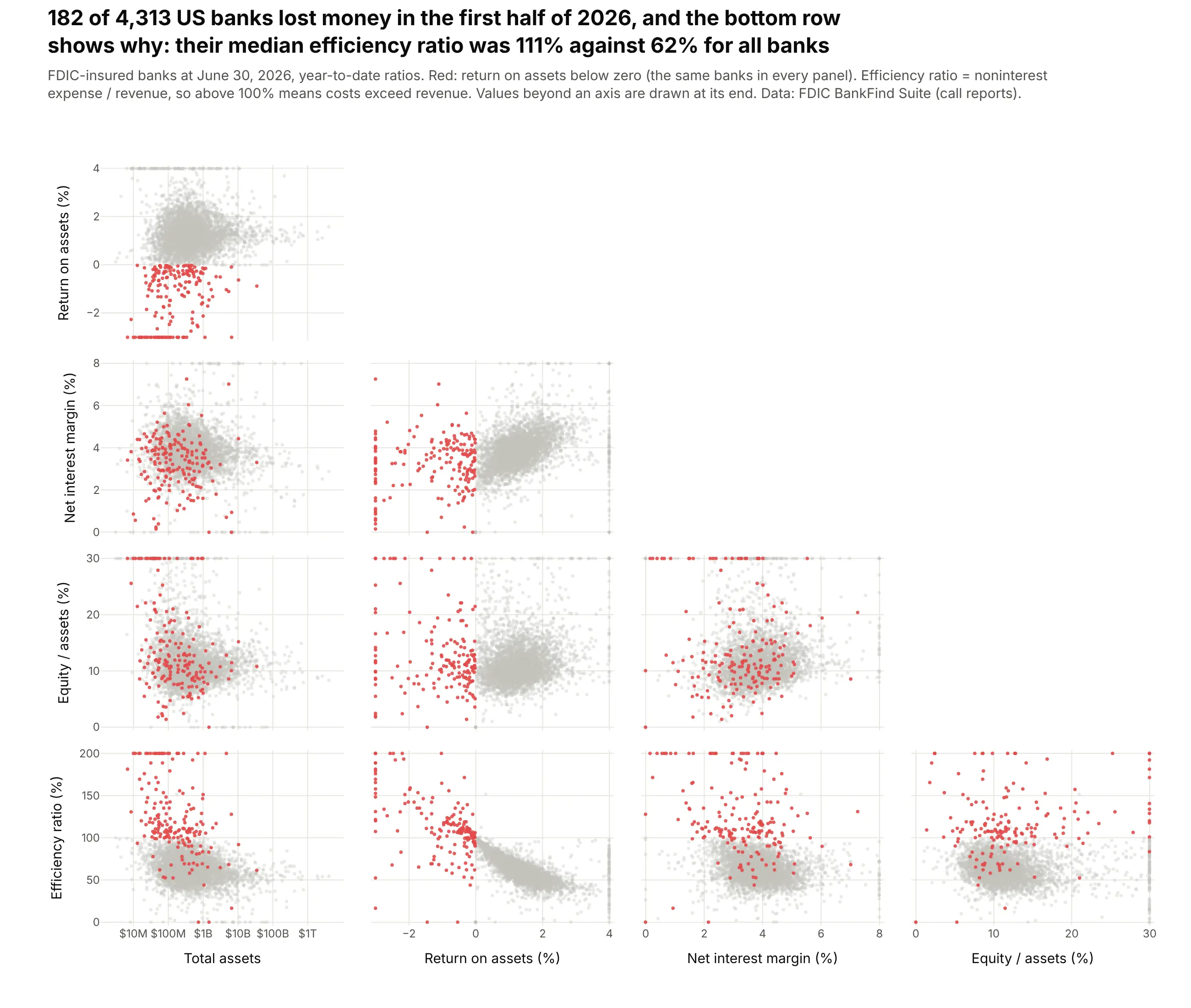
Screening for outliers. The 182 of 4,313 US banks that lost money in the first half of 2026 are highlighted in every panel, and in the bottom row their median efficiency ratio of 111% (costs above revenue) stands apart from 62% for all banks. Data: FDIC BankFind Suite (call reports), June 30, 2026.

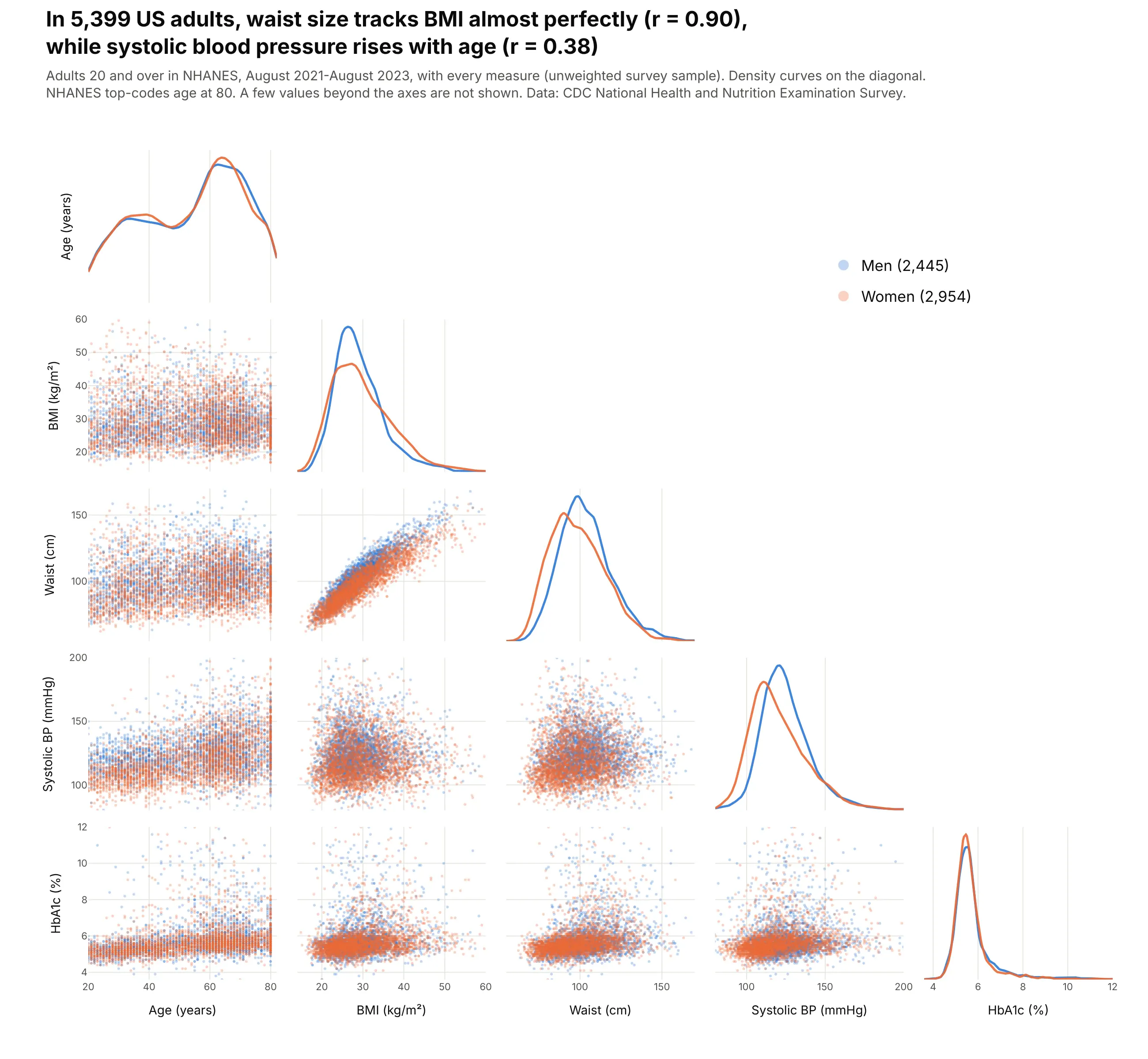
A first look at a clinical cohort. In 5,399 NHANES adults, waist size tracks BMI almost perfectly (r = 0.90), and the density curves on the diagonal show men's systolic blood pressure running higher (median 123 against 117 mmHg). Data: CDC NHANES, August 2021-August 2023.

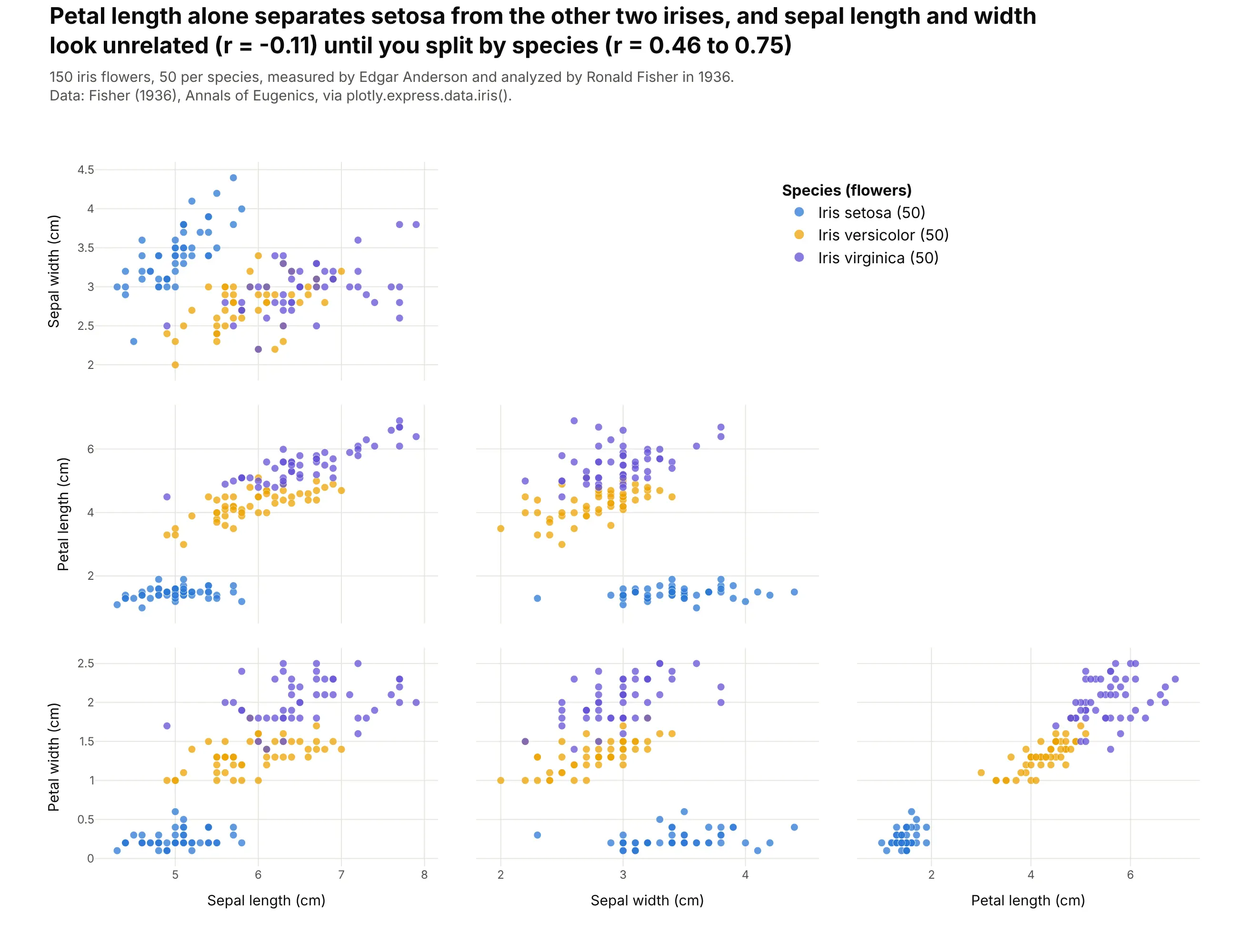
The classic teaching example. In the 150 irises that Edgar Anderson measured and Ronald Fisher analyzed in 1936, petal length alone separates setosa from the other two species, and sepal length and width look unrelated across all flowers (r = -0.11) but rise together within each species. Data: Fisher (1936), Annals of Eugenics, via px.data.iris().

A short history

John Hartigan printed matrices of scatter plots for cluster analysis in "Printer graphics for clustering" (Journal of Statistical Computation and Simulation, 1975), when a plot came out of a line printer one character at a time. Here's what that style looks like, redrawn with Plotly on the NFL Combine data used later in this guide:

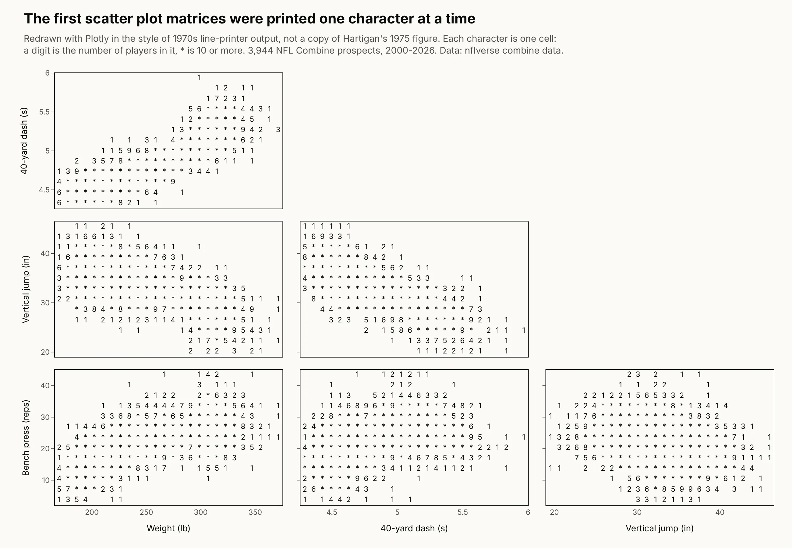
Richard Becker and William Cleveland made the matrix interactive in "Brushing Scatterplots" (Technometrics, 1987), where a rectangle dragged over one panel highlights the same points in all the others. R's pairs() function and seaborn's pairplot (Waskom, 2021) later made it a standard first step in exploratory analysis.

Alternatives to a scatter plot matrix

Here's the same NFL Combine data drawn four ways. Some are better for the question, some worse, some just different:

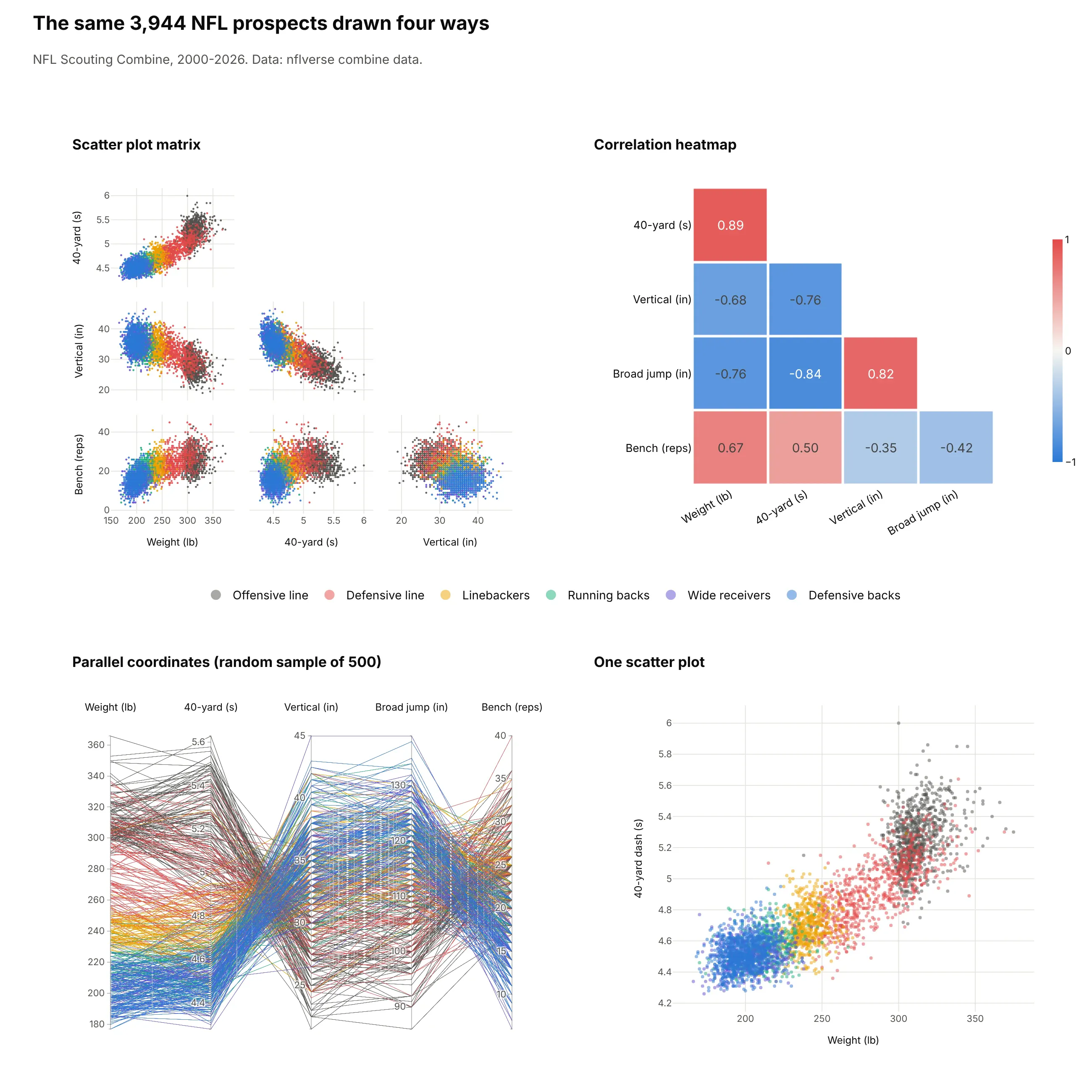
• Correlation heatmap (better for many variables). It replaces each panel with one number, so it fits 20 or more variables, but it hides curves, clusters and outliers. Here weight and 40-yard time correlate at 0.89, and the heatmap can't show that most of that comes from the gap between position groups. See our heatmap guide.
• Parallel coordinates (different). Each player is one line across all five tests, so you can follow individual records, but you can only compare neighboring axes. See our parallel coordinates plot guide.
• One scatter plot (better for one pair). When you already know which pair matters, a single large scatter plot shows it with more room for labels and annotations than a small panel in a grid.

How to make a scatter plot matrix

With AI

ChatGPT, Claude Code, GitHub Copilot, Cursor and other AI tools are excellent at writing Plotly code. Name Plotly in the prompt, spell out the dimensions and their order, the ranges and what color means, and list the checks you want:

With Plotly Studio

Plotly Studio is a desktop app where you point an AI at a dataset and it builds charts and a Dash app around your questions. Ask for a scatter plot matrix the same way:

Show a scatter plot matrix of every bank in this call report file with total assets (log scale), return on assets, net interest margin, equity to assets and efficiency ratio, lower half only. Highlight banks with negative return on assets in red. When I select points in any panel, filter a table of those banks below the chart.

Make a scatter plot matrix in Python or JavaScript

This is the code AI tools write under the hood. In Python, Plotly Express makes one from a DataFrame in one line, where dimensions picks and orders the columns and color splits them into groups:

In JavaScript, plotly.js takes a splom trace with one entry in dimensions per variable:

For histograms or density curves on the diagonal, as seaborn's pairplot draws them, build the grid with make_subplots, as in the NHANES chart above and example 3 below.

Share it

Every Plotly chart has a Share chart button (the cloud icon in its toolbar) that uploads it to Plotly Cloud and gives you a link. Only you can see it until you change its visibility.

For a live app, put the chart in a Dash app and publish it with the Plotly Cloud CLI. Coding agents can run these commands for you:

If your data has to stay in your own cloud or data center, publish to Dash Enterprise instead.

Dos and don'ts

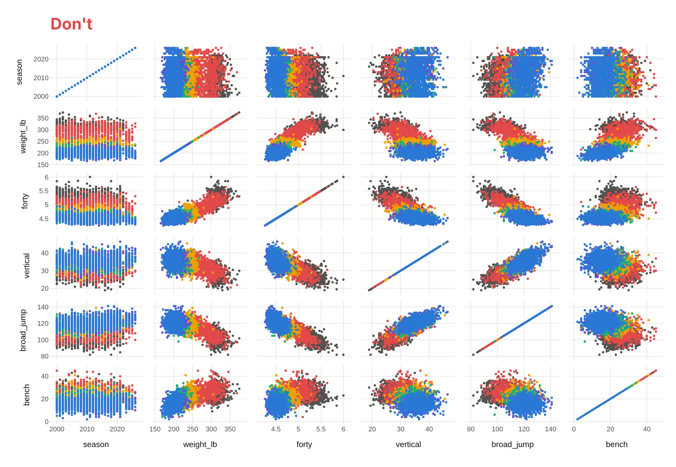
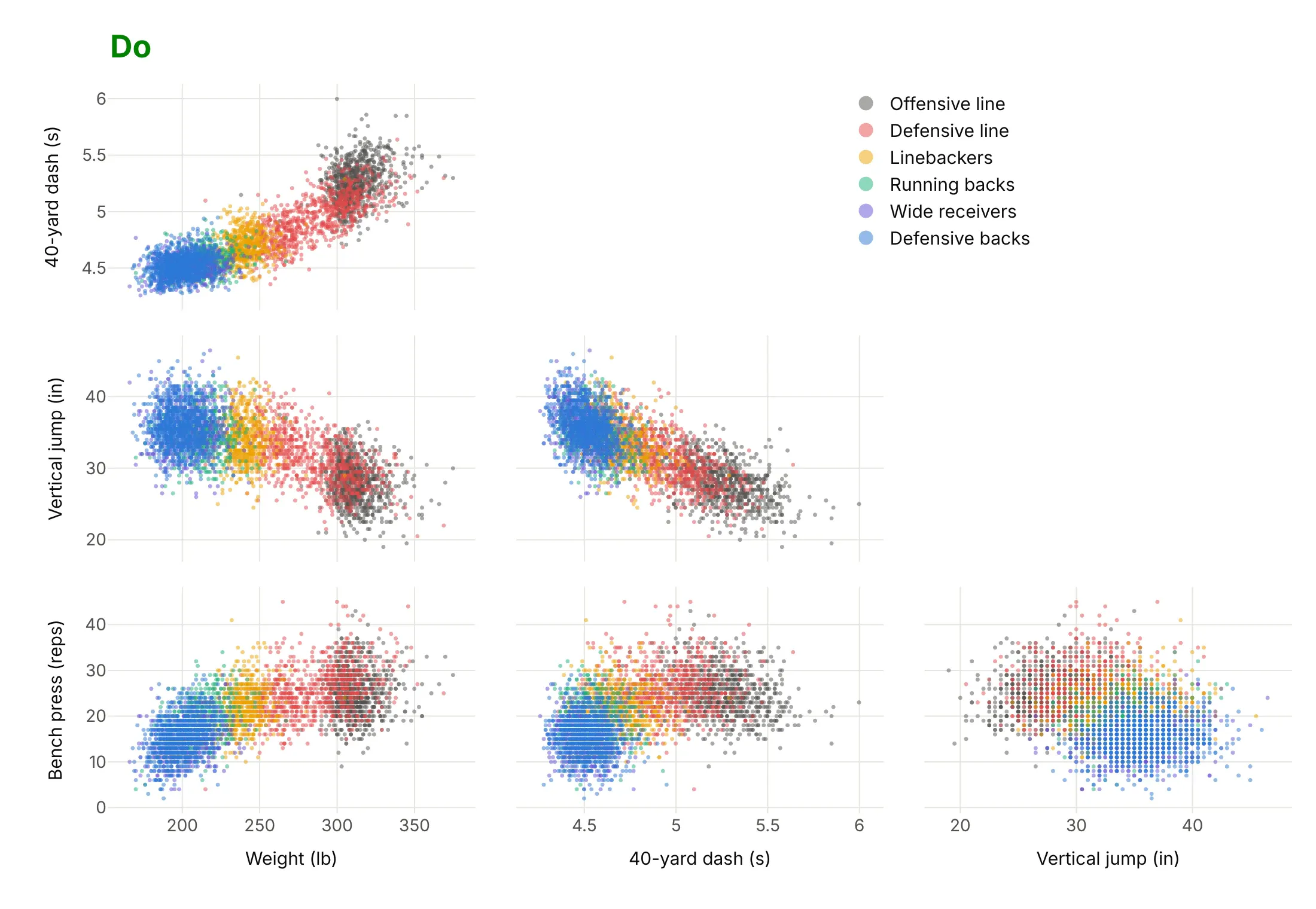
Plotly's defaults show every column you pass and the full matrix, which is fine for exploring. For a published chart, most of the work is deciding what to leave out. Here is the same NFL Combine data both ways, with the same position-group colors in both.

Don't pass every column (including the season), keep raw column names without units, draw the diagonal of straight lines and the mirrored upper half, leave out the legend, or use opaque markers, which here hide the wide receivers under the defensive backs:

Do pick four tests and give them units, show the lower half only, use small faint markers so every group shows through, and put the legend in the empty triangle:

Use color for one thing

Color is the second decision. Here are four options on the same 3,944 players.

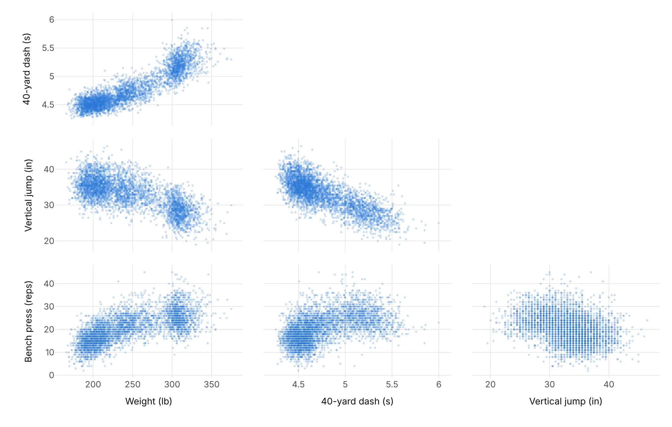
One faint color. Shows density and shape, and it's the right start when there are no groups.

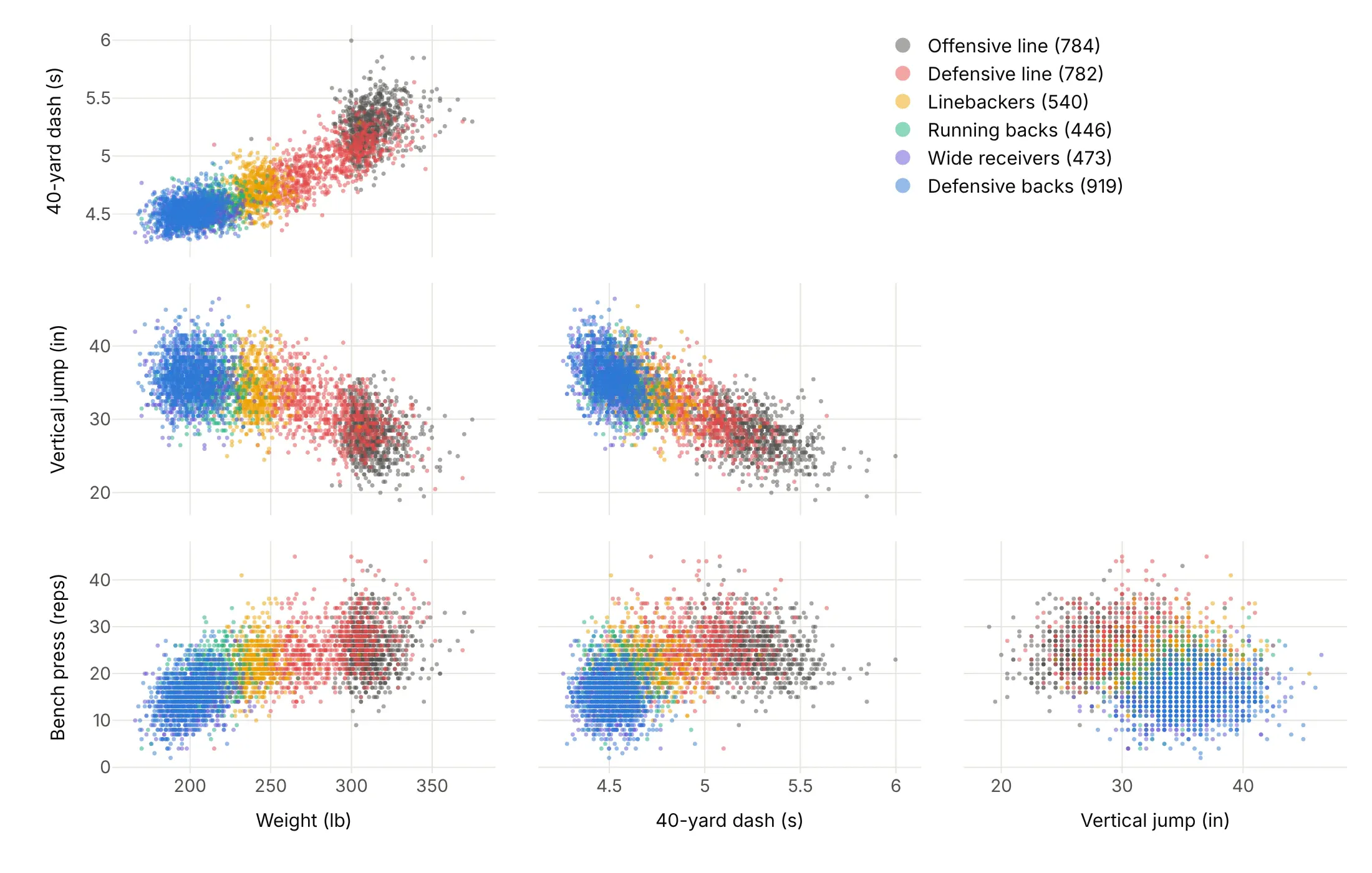
By group. Shows that position explains most of the pattern: linemen are heavy and slow, defensive backs and receivers light and fast.

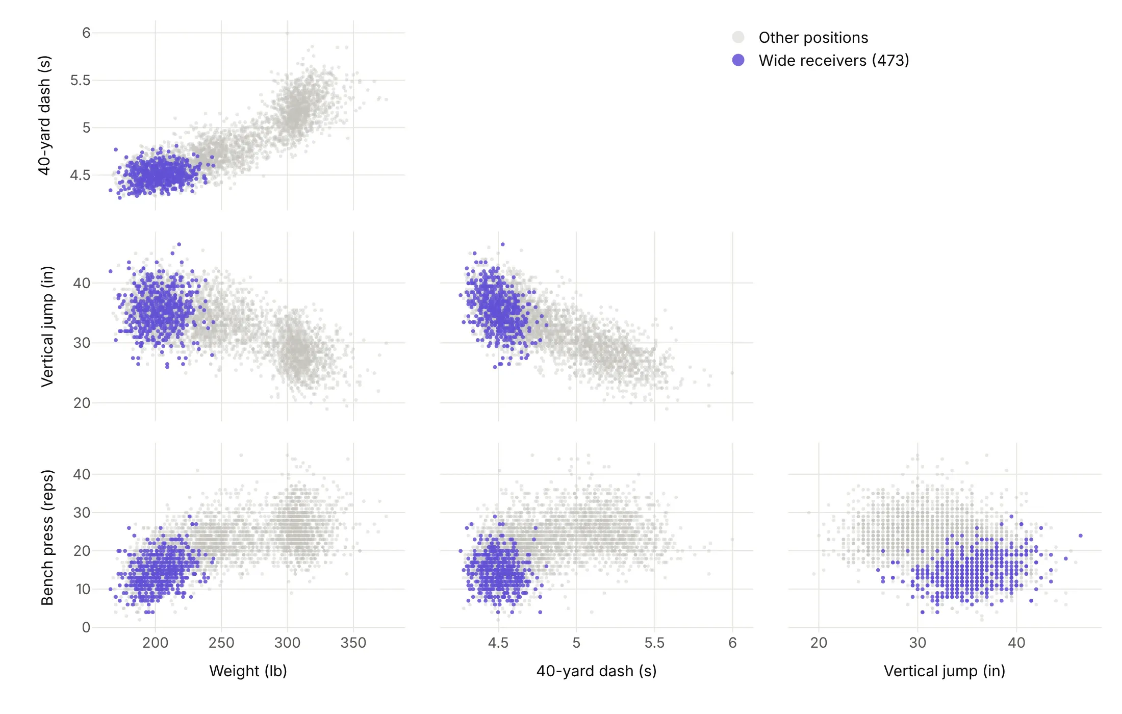
Highlight one group. Answers a question about one group, here where the 473 wide receivers sit in every panel.

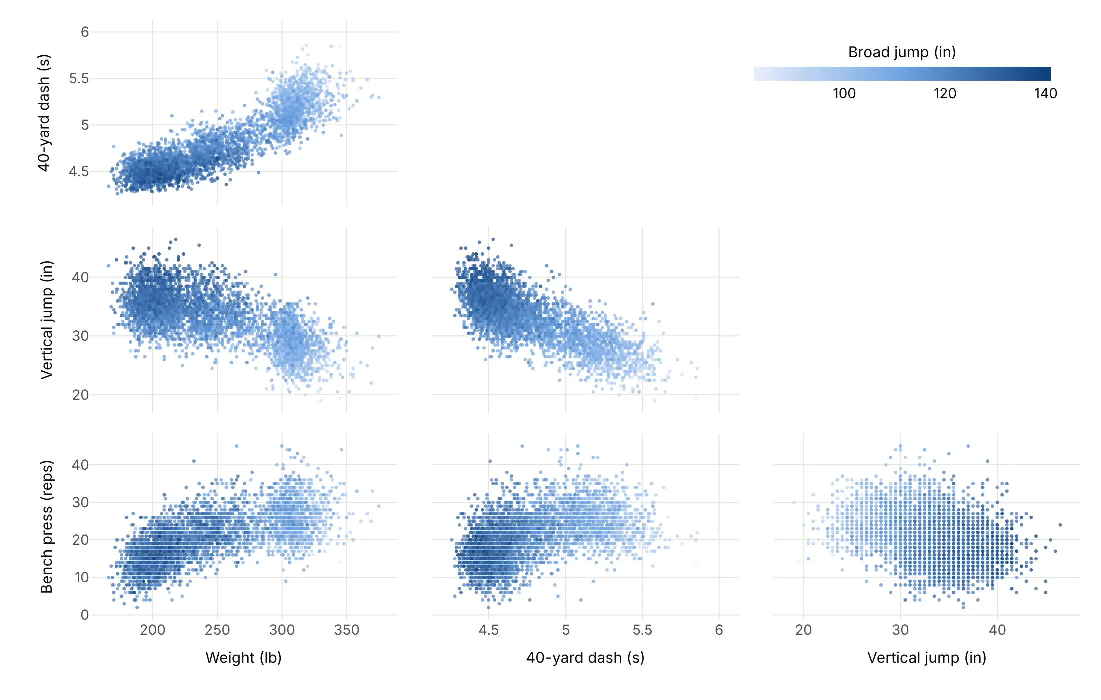
By a fifth variable. A continuous color adds a measure that has no panel, here the broad jump, which rises as the 40-yard time falls.

Checklist

Do

• Write a title that states the takeaway, usually a correlation or a group difference.
• Pick and order the dimensions on purpose, so related variables sit next to each other.
• Hide the upper half and the diagonal (showupperhalf=False, diagonal.visible=False) and put the legend or colorbar in the empty triangle.
• Put units in the dimension labels and fix axis ranges so a few outliers don't squash everything else.
• Use small, faint markers (size 2-4, opacity 0.2-0.5) when there are thousands of points.

Don't

• Pass every column, because IDs, years and near-duplicate columns waste panels.
• Trust a correlation without looking at the panel. Weight and 40-yard time correlate at 0.89 across all players, but only 0.16 to 0.71 inside a position group.
• Use a rainbow for groups or a continuous scale.
• Plot rounded values raw. Jitter them by at most half the rounding step, or aggregate them.

Options to customize

These are the go.Splom (and px.scatter_matrix) options that matter most. The full list is in the Plotly scatter plot matrix documentation.

1. dimensions (px: a list of columns): the variables and their order. Pick and order them on purpose.
2. dimensions[].label, .values: the axis title and the data. Put units in the label.
3. dimensions[].visible: hides a dimension but keeps its data, for toggling variables in a Dash app.
4. dimensions[].axis.type, .matches: the axis type for that dimension, or links its x and y ranges.
5. showupperhalf, showlowerhalf: show either half of the matrix. Hide the mirrored half.
6. diagonal.visible: shows the diagonal panels, which most charts turn off.
7. marker.color, colorscale, cmin, cmax, colorbar: one color, or a number mapped to color.
8. marker.size, opacity: point size (a number or an array) and transparency. Small and faint for big data, or size by count.
9. selectedpoints, selected, unselected: a stored selection and the styles in and out of it, to show linked brushing in a static image.
10. text, hovertemplate, customdata: hover content, such as the name of each record.
11. xaxes, yaxes: which axes each dimension uses, to put several matrices in one figure.
12. layout.xaxisN, layout.yaxisN: the axes of dimension N (type, range, tickvals), for log scales and fixed ranges.
13. layout.dragmode: select or lasso for linked brushing.
14. px.scatter_matrix(color=..., symbol=...): one trace per group with a legend, the fastest way to color by group.

More scatter plot matrix examples

Nine more scatter plot matrices built from real public data, each with its source, the technique that makes it work and a prompt to rebuild it.

1. Energy use in 22,127 New York City buildings

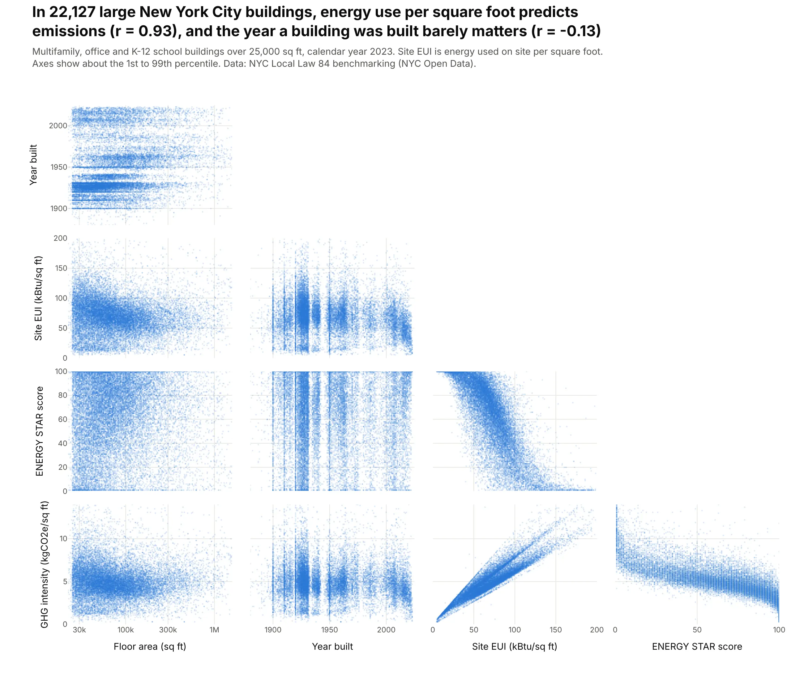
Buildings over 25,000 square feet in New York report their energy use every year. Across 22,127 multifamily, office and school buildings in 2023, energy use per square foot predicts emissions per square foot almost exactly (r = 0.93), while the year a building was built barely matters (r = -0.13). Data: NYC Local Law 84 benchmarking, 2023 (NYC Open Data).

Tip: with 22,000 points per panel, markers of size 2.5 at opacity 0.18 turn overplotting into a density picture, and fixed ranges at about the 1st and 99th percentiles drop the data-entry outliers.

2. US wind turbines grew in every dimension

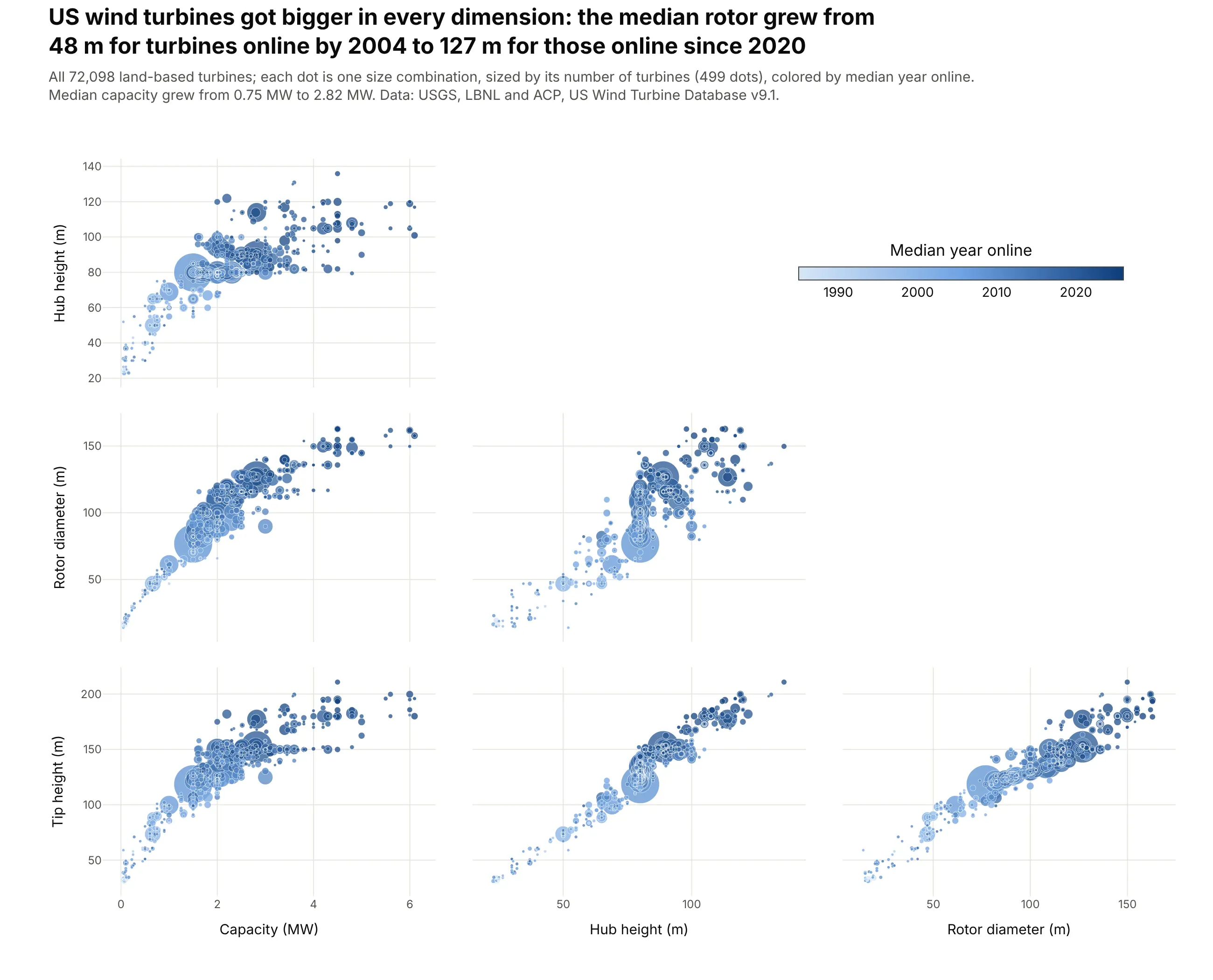
The median rotor on a US wind turbine grew from 48 m for turbines online by 2004 to 127 m for those online since 2020, and the median turbine from 0.75 MW to 2.82 MW. Light old turbines sit in the bottom-left of every panel and dark new ones at the top right. Data: USGS, LBNL and ACP, US Wind Turbine Database v9.1.

Tip: 72,098 turbines are only 499 distinct size combinations, so each dot is a combination sized by np.sqrt(count), with the biggest dots drawn first so small ones stay visible.

3. Six US equity factors, 63 years of monthly returns

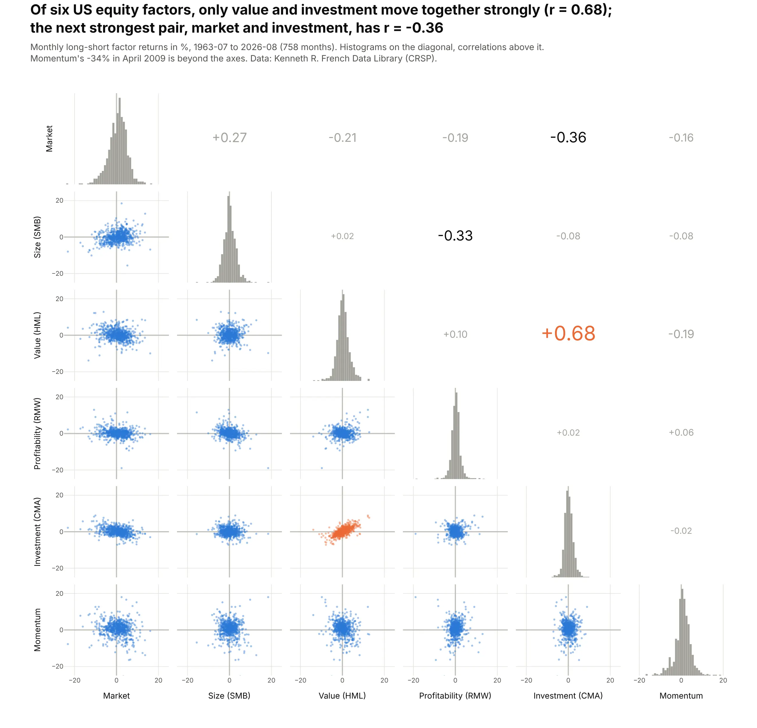
Quants check how factors co-move before they combine them. Over 758 months since July 1963, value (HML) and investment (CMA) are the only pair with a strong correlation (r = 0.68); the next strongest, market and investment, is -0.36. Data: Kenneth R. French Data Library (CRSP).

Tip: a make_subplots grid with go.Histogram on the diagonal, go.Scattergl below it and the correlation as text above it, with font size growing with |r|.

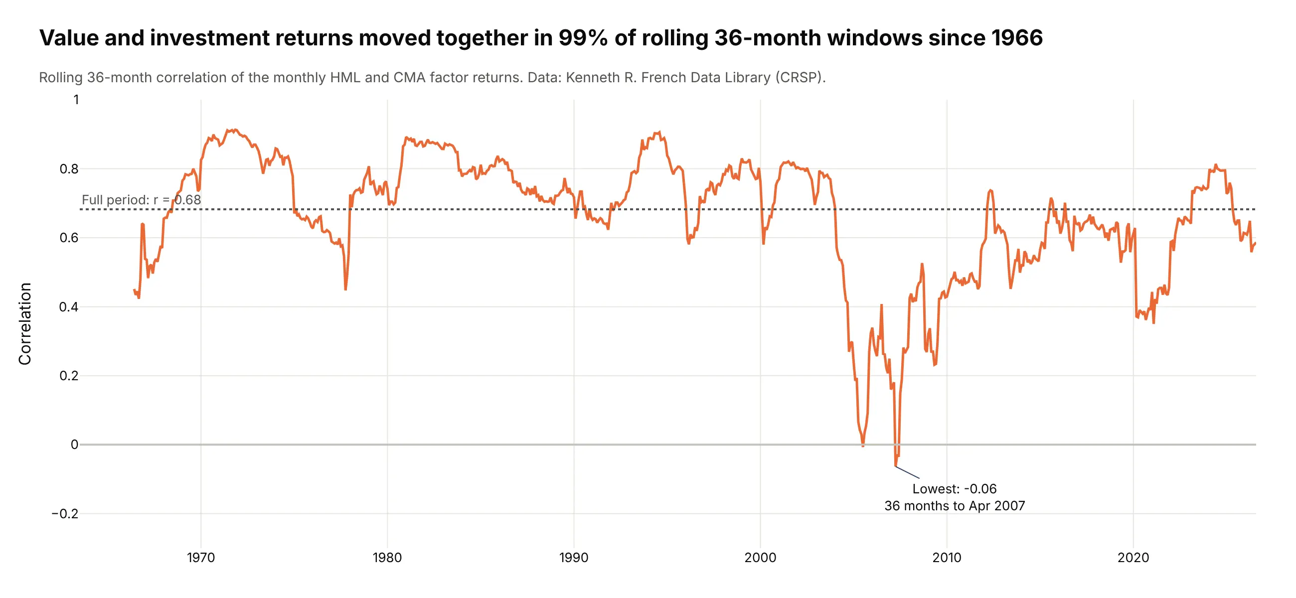
Another way to see it: a rolling 36-month correlation shows the pair is not constant. It stayed positive in 99% of windows, but fell to -0.06 in the 36 months to April 2007.

4. Daily moves in US Treasury yields

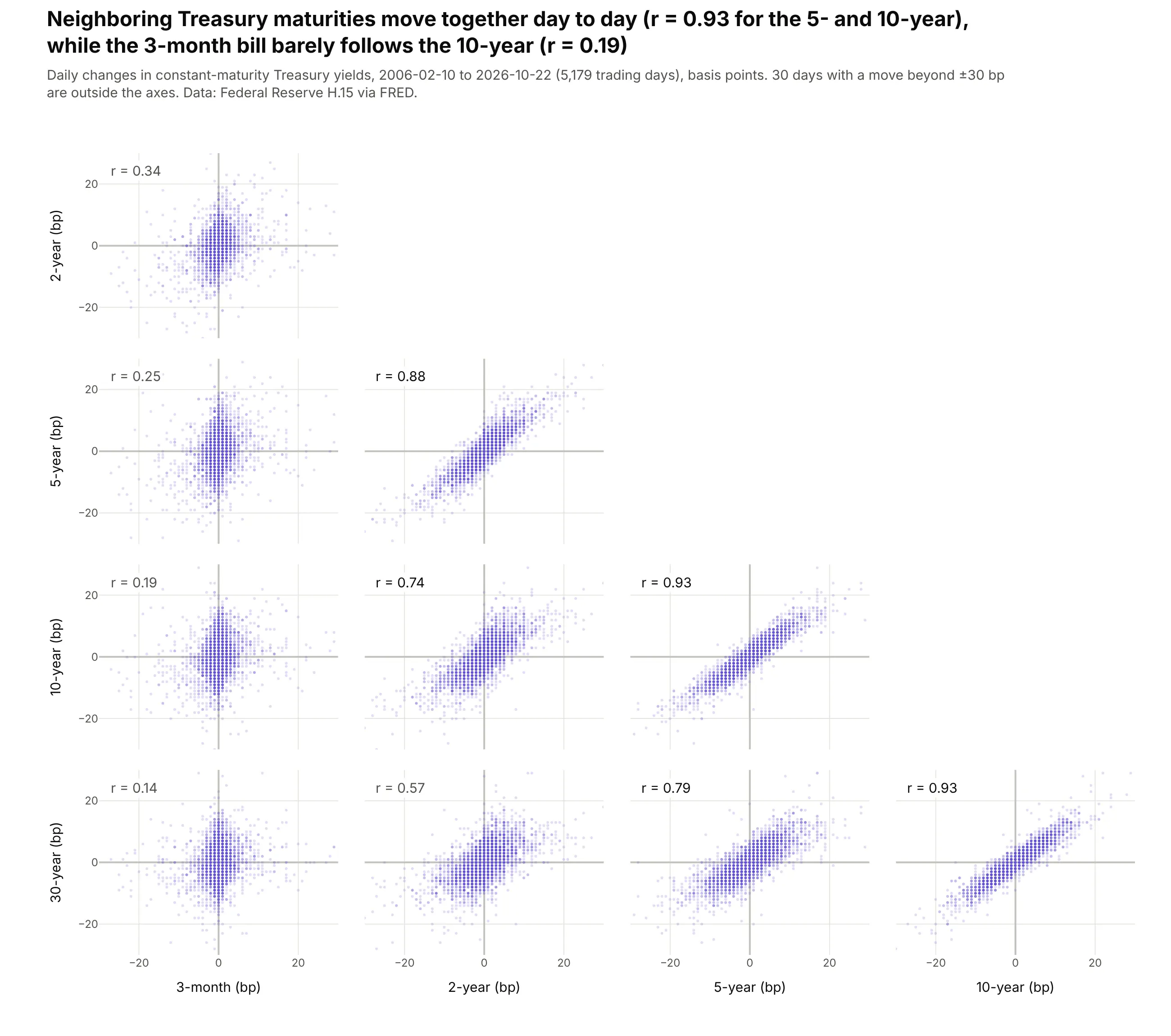
With maturities in order, the matrix reads like the yield curve. Over 5,179 trading days since 2006, the 5- and 10-year yields moved together (r = 0.93), and the link fades with distance until the 3-month bill barely follows the 10-year (r = 0.19). Data: Federal Reserve H.15 via FRED.

Tip: each panel's r is an annotation anchored to that panel's axes with xref="x2 domain" and yref="y4 domain", and every axis shares the same ±30 bp range.

5. Eight health measures across 2,956 US counties

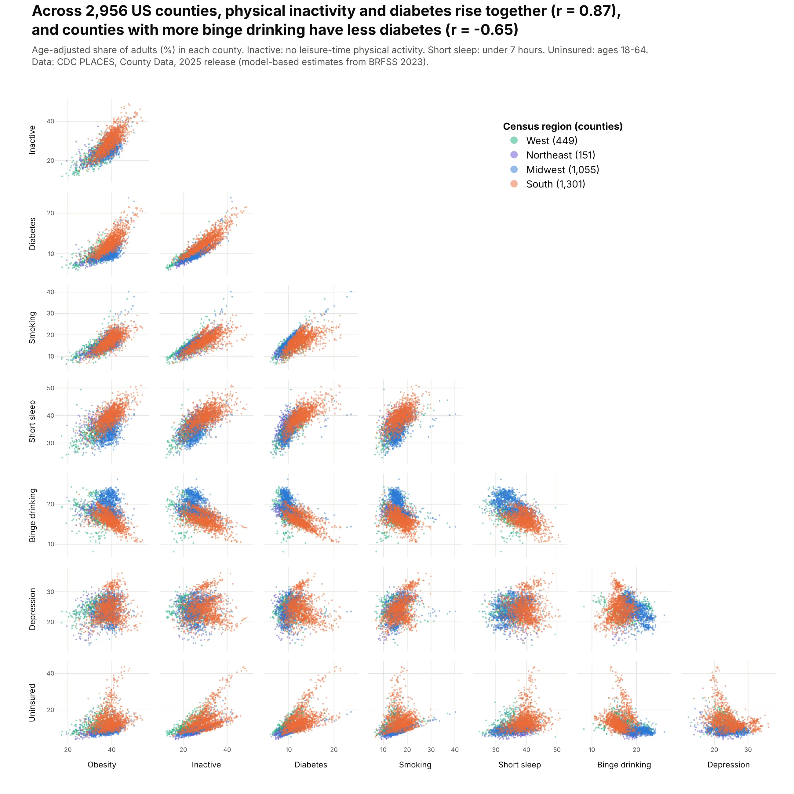
Eight measures make 28 panels, about the most a matrix can show. Across 2,956 counties, physical inactivity and diabetes rise together (r = 0.87), and counties with more binge drinking have less diabetes (r = -0.65), with the Midwest as its own cluster. Data: CDC PLACES, County Data, 2025 release.

Tip: short dimension labels, nticks=4 and size 10 tick labels keep 28 small panels readable.

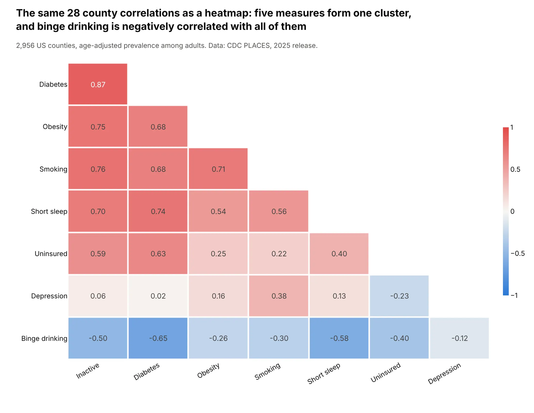
Another way to see it: a correlation heatmap with the measures ordered by cluster puts the same 28 numbers in one compact grid and shows that binge drinking is negatively correlated with all seven other measures.

6. Gasoline car fuel economy since 1984

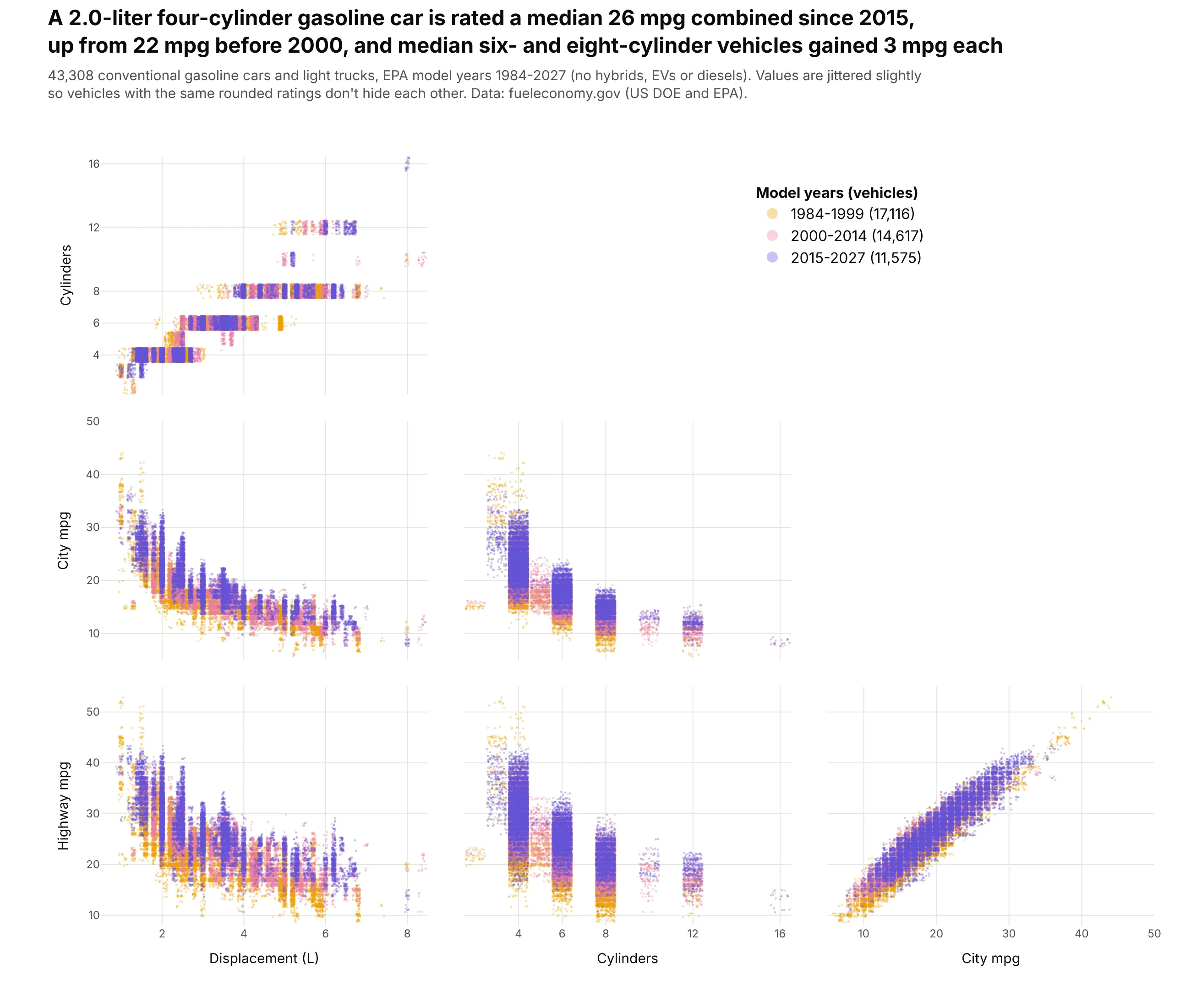
EPA ratings are rounded, so 43,308 vehicles stack onto a few hundred points. Jittered, the eras separate: a 2.0-liter four-cylinder car is rated a median 26 mpg combined since 2015, up from 22 mpg before 2000, and median six- and eight-cylinder vehicles gained 3 mpg each. Data: fueleconomy.gov (US DOE and EPA).

Tip: jitter each variable by at most half its rounding step (0.05 L, 0.45 cylinders, 0.4 mpg) with a fixed seed, and say so in the subtitle.

7. Stars within 100 parsecs of the Sun

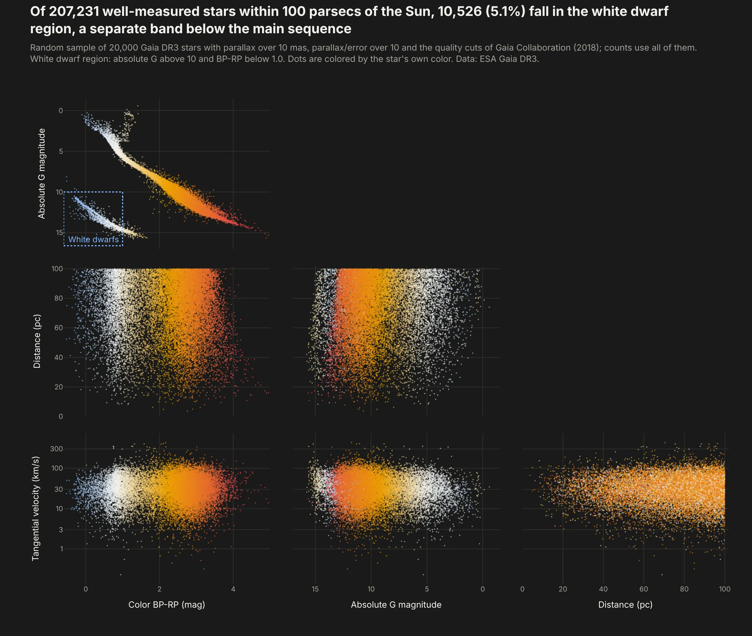
The color-magnitude panel is a Hertzsprung-Russell diagram. Of 207,231 well-measured stars within 100 parsecs in Gaia DR3, 10,526 (5.1%) fall in the white dwarf region, a separate band below the main sequence. The distance panels show Gaia's brightness limit, because the faintest stars are only detected close to the Sun. Data: ESA Gaia DR3.

Tip: the magnitude axis is reversed (range=[17, -1.5]) because brighter stars have smaller magnitudes, and each dot is colored by its own BP-RP color on a blue-white-orange scale.

8. NFL Combine results by position

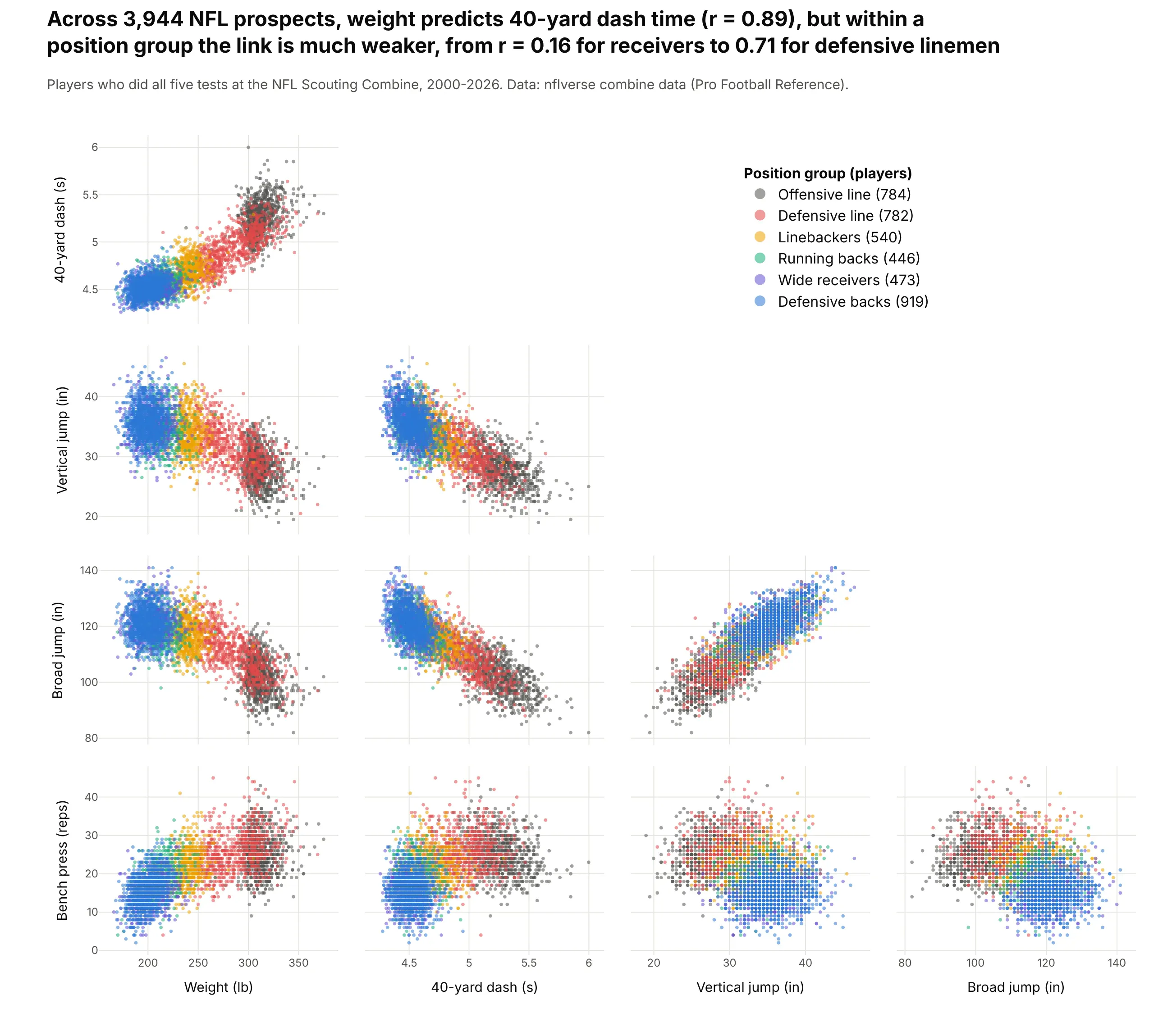
Across 3,944 prospects since 2000, weight predicts 40-yard dash time well (r = 0.89). Colored by position, the matrix shows that most of that comes from the difference between groups, because within a group the correlation ranges from 0.16 for wide receivers to 0.71 for defensive linemen. Data: nflverse combine data (Pro Football Reference).

Tip: one trace per position group, so a click on the legend hides a group and a double-click isolates it, and player names in text for the hover.

9. Six benchmark scores for 4,565 open LLMs

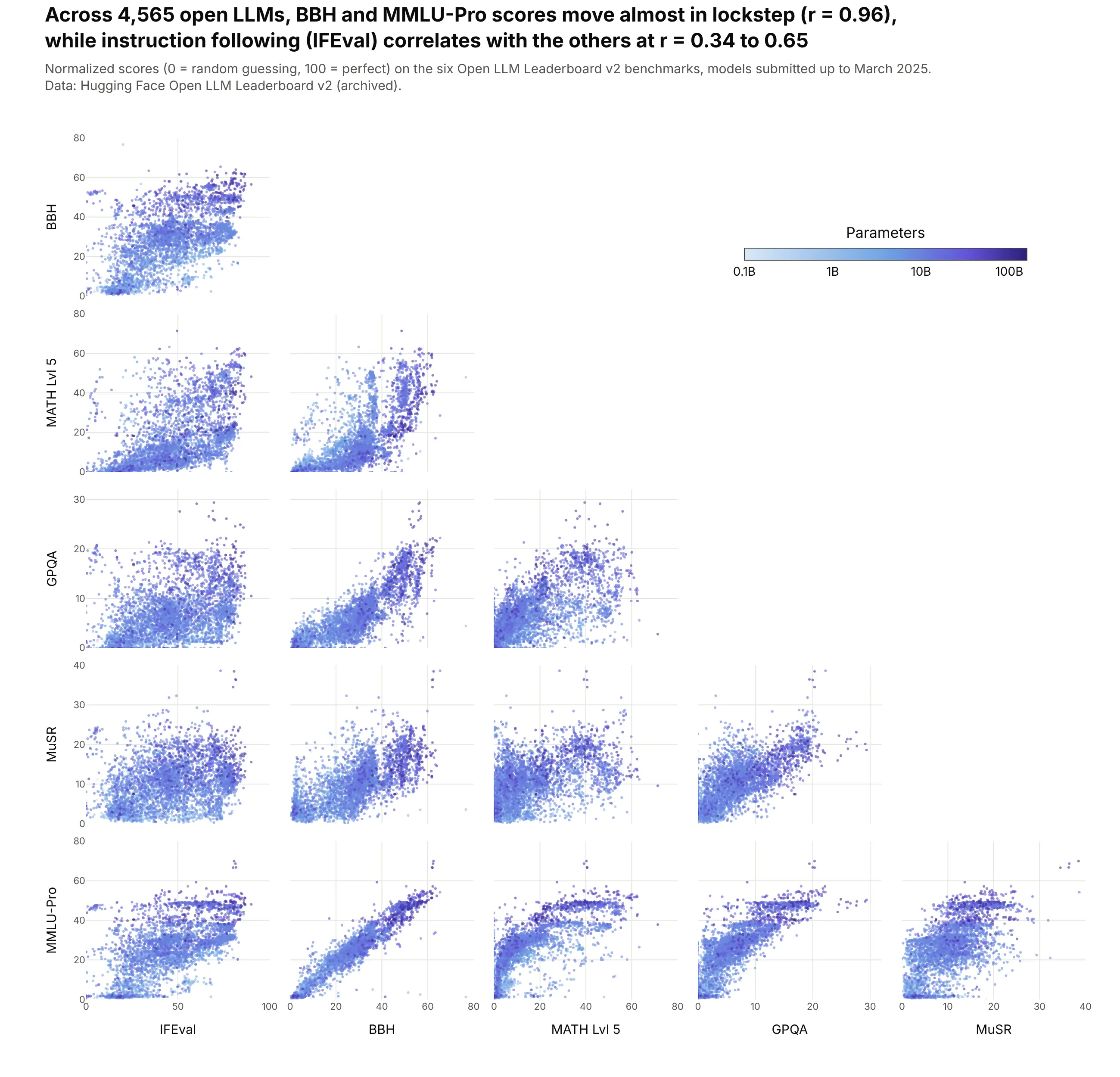
Benchmarks that move together measure similar things. Across 4,565 open models on Hugging Face's Open LLM Leaderboard, BBH and MMLU-Pro move almost in lockstep (r = 0.96), while instruction following (IFEval) correlates with the other five at only 0.34 to 0.65. Data: Hugging Face Open LLM Leaderboard v2 (archived).

Tip: color is log10 of the parameter count, with colorbar tickvals at log10 values and ticktext like "1B" and "10B", and the largest models drawn last.

10. Approved drugs against Lipinski's rule of five

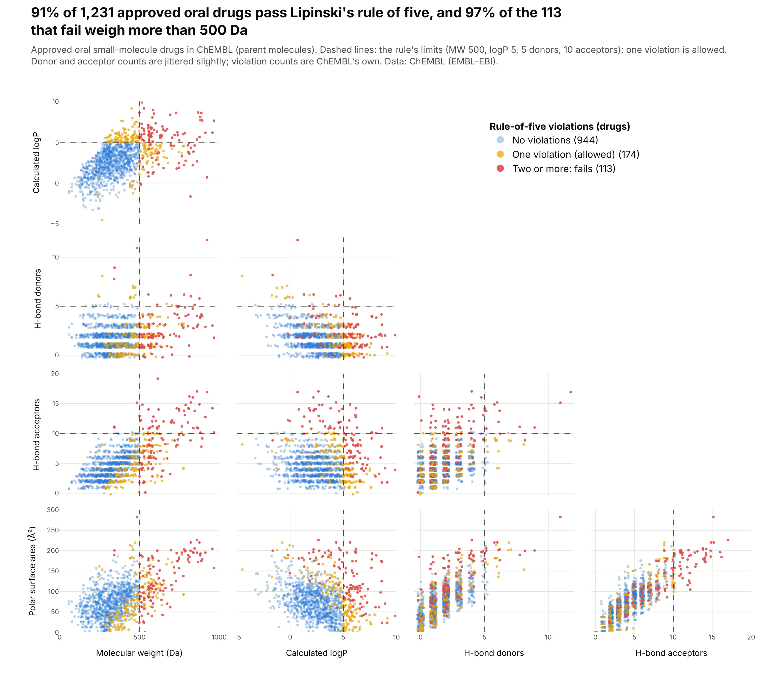
Medicinal chemists screen compounds against Lipinski's rule of five, which checks four properties at once. Of 1,231 approved oral drugs in ChEMBL, 91% pass (one violation is allowed), and drawing the four limits in every panel shows that nearly all of the 113 drugs that fail are heavier than 500 Da. Data: ChEMBL (EMBL-EBI), approved small molecules.

Tip: draw the limits as shapes anchored to each panel's own axes (xref="x2", yref="y4 domain"), and add a little jitter to the integer donor and acceptor counts so identical values don't stack.