
Chris Parmer
November 18, 2026
Periodic Table of Investment Returns (Quilt Charts) - A Complete Guide
TL;DR
- A periodic table of investment returns has one column per year. In each column the asset classes are ranked from the best return (top) to the worst (bottom), each class keeps one fixed color in every column so you can follow it across years, and each cell shows the class name and its return. It makes one point at a glance: the leader changes from year to year.
- Periodic tables of returns are also known as quilt charts, asset allocation quilts and returns quilts, and are similar to bump charts and heatmaps. The best-known one is Callan's Periodic Table of Investment Returns, which Callan LLC created in 1999 (callan.com); the charts in this guide are our own, built from public data.
- The field's conventions: calendar-year total returns (income reinvested), the same eight to ten asset classes in every column, fixed colors, best at the top, full years only. Advisers and consultants use it to explain diversification, and read it next to a drawdown chart and an efficient frontier. It does not prove that last year's winner will fall: in 25 years of S&P 500 sector data the rank correlation from one year to the next was -0.03.
- You can make a periodic table of returns with Plotly from a heatmap trace with a stepped colorscale, so that the class decides the color of each cell. This guide is educational and is not investment advice.
What is a periodic table of investment returns?
This is a periodic table of investment returns:
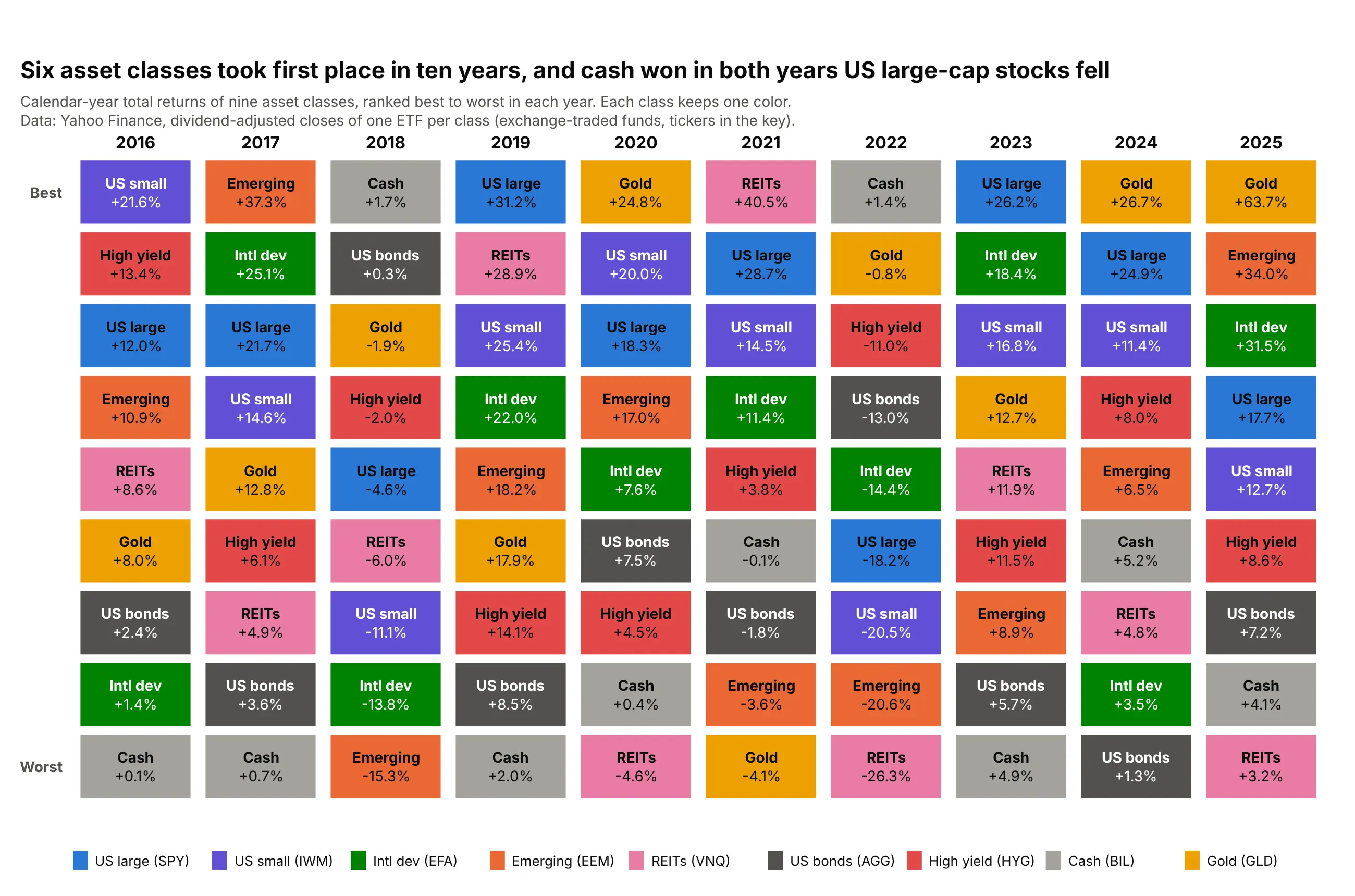
Data: Yahoo Finance, dividend-adjusted closes (total return) of one exchange-traded fund (ETF) per class, December 31, 2015 to December 31, 2025: SPY (S&P 500), IWM (Russell 2000 small caps), EFA (developed markets outside North America), EEM (emerging markets), VNQ (real estate investment trusts, REITs), AGG (US investment-grade bonds), HYG (US high-yield bonds), BIL (1-3 month Treasury bills, "cash") and GLD (gold).
How do you read a periodic table of returns? In the example above, notice these things:
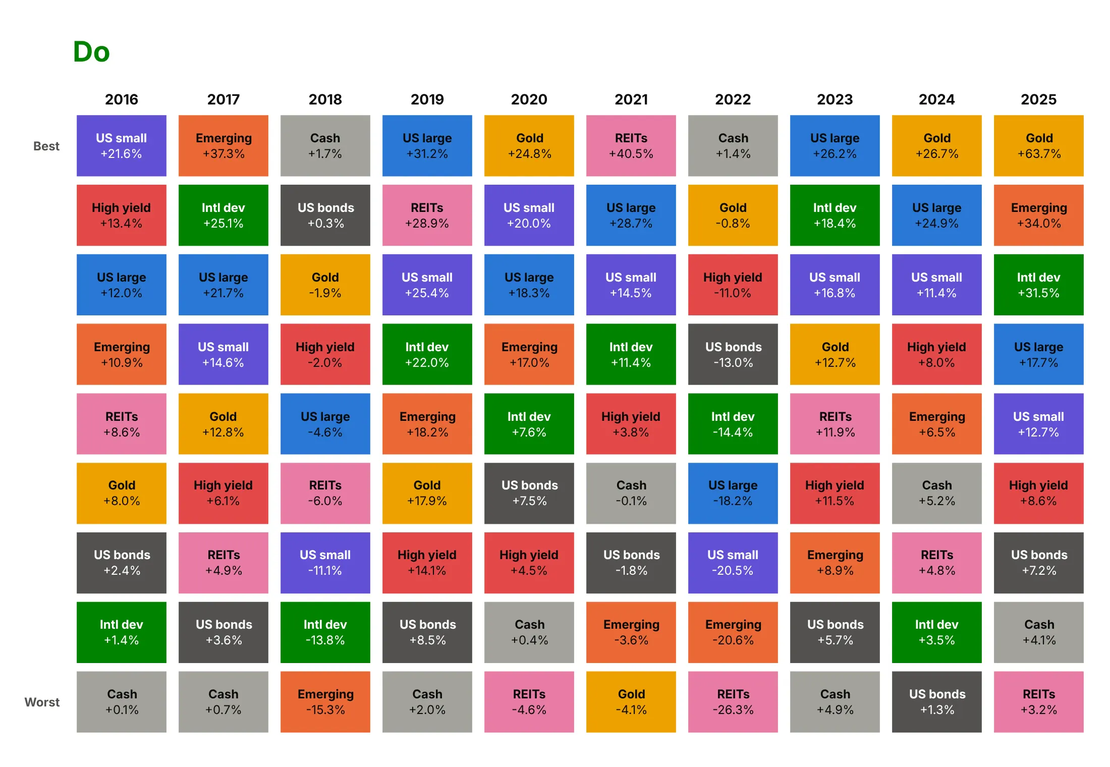
- Each column is one calendar year, and the nine classes are ranked by that year's return, best on top. In 2025 gold returned 63.7% and sat first, while REITs returned 3.2% and sat last.
- Each class keeps one color, so you can follow it across years. REITs (pink) were first in 2021 at 40.5% and last in 2022 at -26.3%.
- Six different classes finished first in ten years, and no class finished first more than three times (gold, in 2020, 2024 and 2025). The top row has no streak longer than two years.
- Cash (gray) finished first in 2018 and 2022, the only two years in this period when US large-cap stocks lost money (-4.6% and -18.2%), and last in 2016, 2017, 2019 and 2023.
It's often used for charts like these:
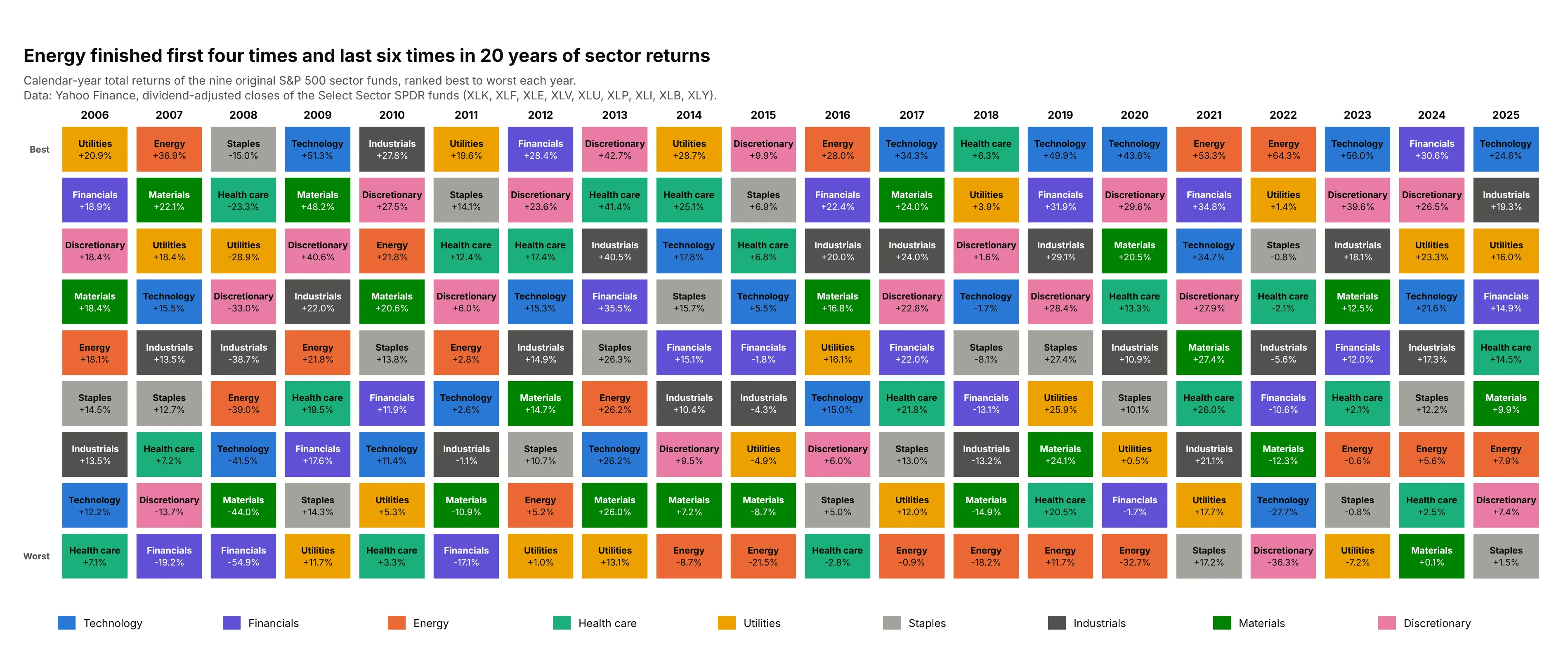
Sector rotation. Equity analysts rank the 11 sectors of the S&P 500 the same way: Energy finished first four times and last six times in 20 years, and Technology finished first six times. Data: Yahoo Finance, nine Select Sector SPDR funds, 2006 to 2025.
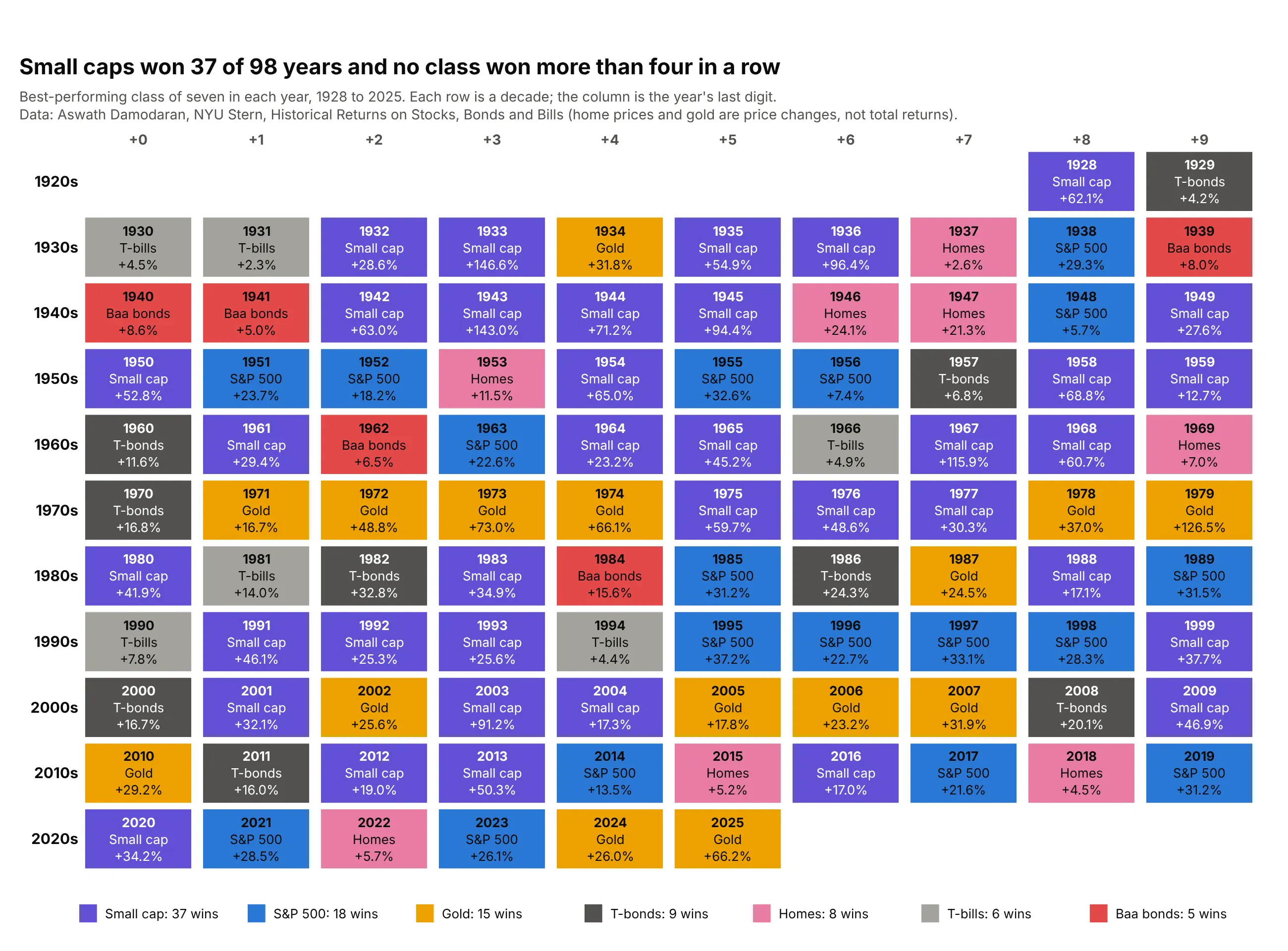
A century of winners. Stretched to 98 years and seven classes, the same idea shows each year's winner only: small caps won 37 times, the S&P 500 18 times and gold 15 times, and no class won more than four years in a row. Data: Aswath Damodaran, NYU Stern, annual returns 1928 to 2025.
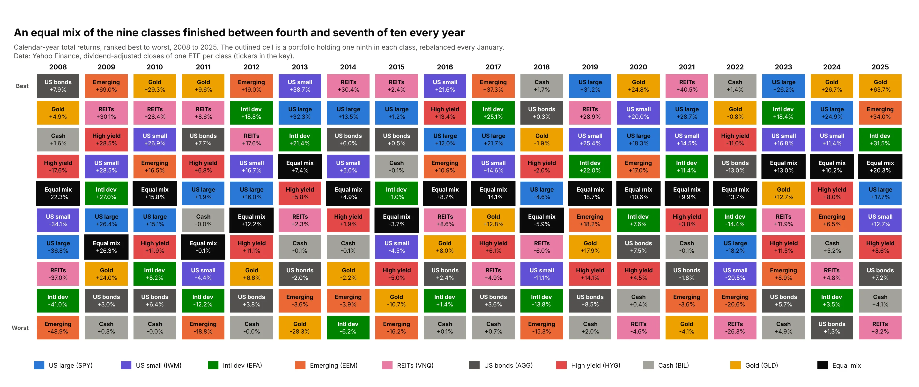
Showing diversification. Advisers outline a diversified portfolio in the table to show that it is rarely the best and never the worst: an equal mix of the nine classes finished between fourth and seventh of ten in every one of 18 years. Data: Yahoo Finance, the nine ETFs of the first example, 2008 to 2025.
A short history
The Callan Periodic Table of Investment Returns was created by Jay Kloepfer in 1999 at Callan, an investment consulting firm, and ranks the annual returns of nine asset classes from best to worst, using industry-standard indices as proxies for each class (Callan). Kloepfer says its appeal is that it can be "understood at a glance", and it is Callan's work and trademark: the data, classes and styling in this guide are ours. The idea has many descendants, such as Monevator's asset allocation quilt for UK investors (Monevator) and Portfolio Charts' returns quilt (Portfolio Charts), and they all rest on the argument that Harry Markowitz made for diversification in 1952 (Markowitz) and that Brinson, Hood and Beebower followed in 1986 by studying how much of the returns of large pension funds came from their mix of asset classes (Brinson et al.).
To show the idea as it would have looked in the years before the table appeared, here is a quilt of 1979 to 1998 that we drew from Damodaran's public data. It is not Callan's table: the classes, data and design are different.
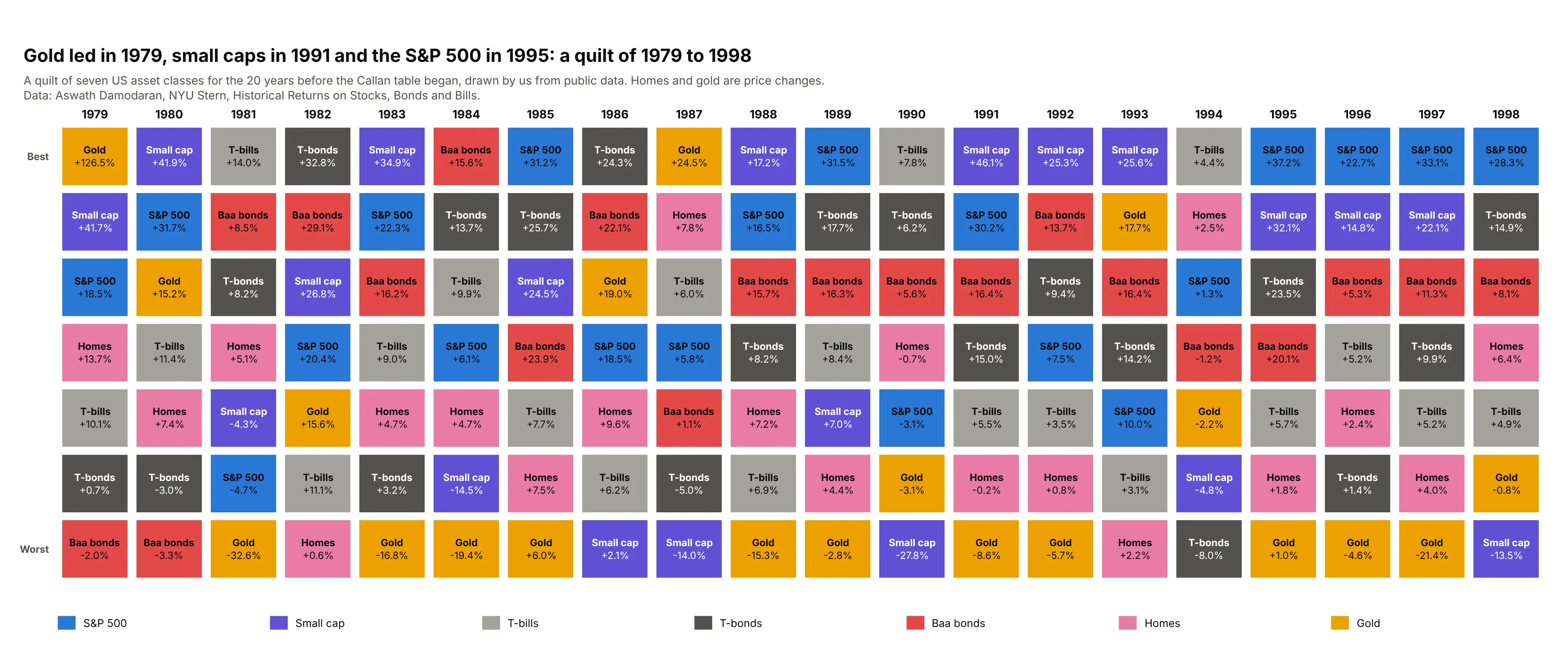
Data: Aswath Damodaran, NYU Stern, Historical Returns on Stocks, Bonds and Bills (home prices and gold are price changes, not total returns).
How a periodic table of returns is built
The chart looks like a heatmap, but it follows its own rules, and most mistakes come from the details around those rules. This section explains them for a reader who has not worked with returns before.
One column is a sorted bar chart
For one year, take the return of each asset class, sort the classes from best to worst, and draw each bar as a same-size cell with the class name and its return. Stack the cells into a column and put one column per year side by side:
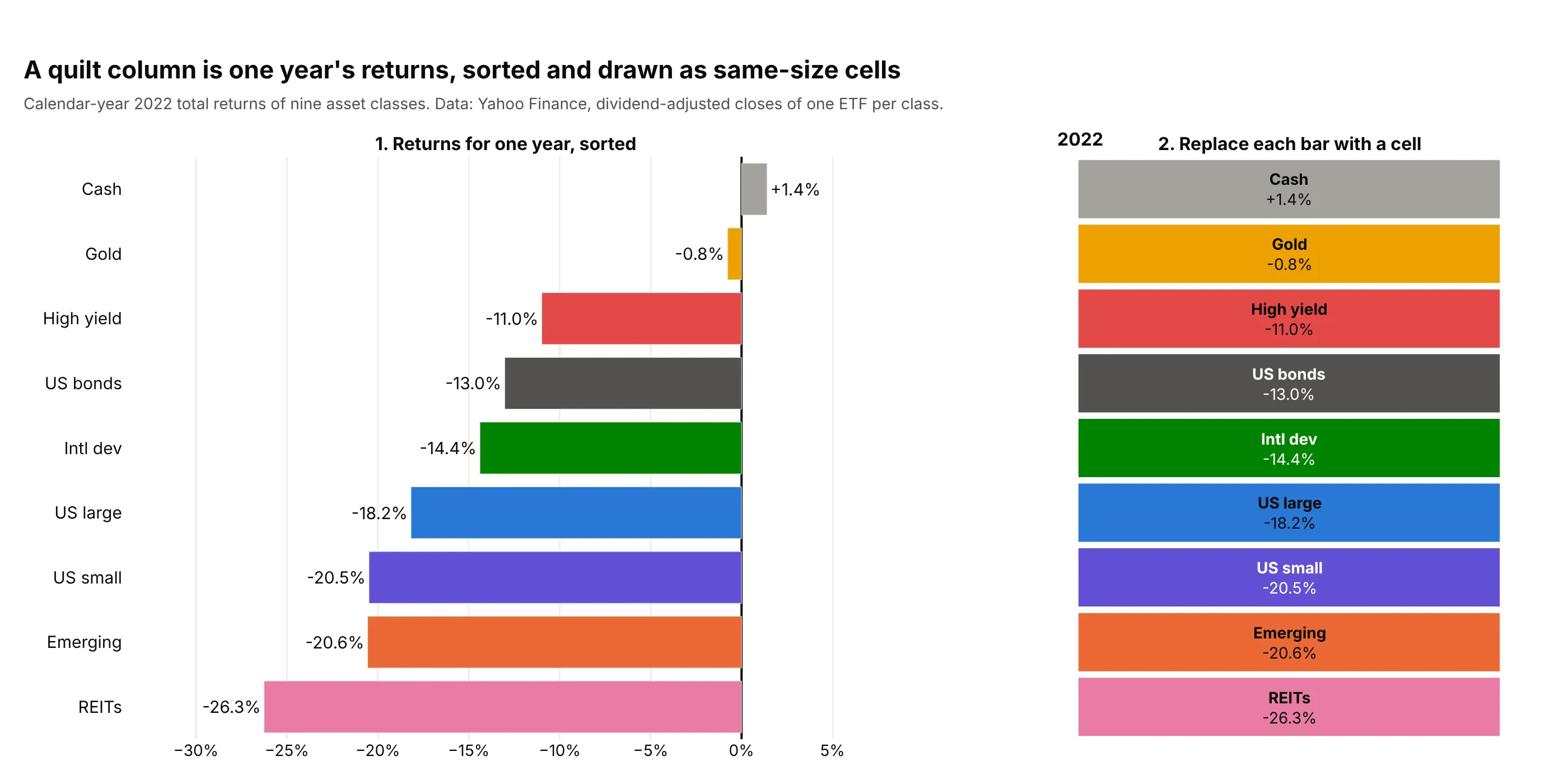
Data: Yahoo Finance, dividend-adjusted closes of one ETF per class, December 31, 2021 to December 31, 2022.
The cells are all the same size, which is why the table shows rank clearly and size poorly. In 2022 the gap between first and second place was 2.2 points (cash at 1.4% and gold at -0.8%), and the gap between second and last was 25.5 points, but the two steps look the same on the table.
What "total return" means
A total return is the change in an investment's value including the income it paid, with that income reinvested: dividends for stocks, interest for bonds and bills, rent distributed by REITs. A price return leaves the income out, which understates the return of anything that pays income, such as bonds. The convention in the field is total return, and the data here come from dividend-adjusted closing prices, which already include the reinvested income.
Calendar years, indices and ETFs
The columns are calendar years: the return from the last trading day of one December to the last trading day of the next. A year that is not over, such as 2026 in November, does not belong next to full years unless it is labeled as partial.
Consultants such as Callan use market indices (for example the S&P 500) as the measure of each asset class. An index has no fees and can't be bought, so this guide uses one exchange-traded fund (ETF) per class, whose returns are after the fund's expenses. For the S&P 500 the difference is small: Damodaran's S&P 500 series with dividends and the SPY fund differ by at most 0.42 percentage points in any year from 2008 to 2025 (in 2009).
Why each class keeps one color
The color is the only thing that lets a reader follow a class across years without reading every cell, so it must never change with the return or the rank. That is the difference from a heatmap, where the color tells you how large the value is. Because Plotly's heatmap trace colors by value, the chart is drawn by giving each class an integer and a stepped colorscale, so each integer maps to one fixed color (the code is below).
What the table can and cannot say about the future
Reading the table, many people expect that the class at the top will drop and the class at the bottom will recover, an idea called mean reversion: results moving back toward their long-run average. Academic research does find some predictable patterns, but of different kinds: over three to 12 months, winners tend to keep winning (Jegadeesh and Titman 1993), and over three to five years, past losers have tended to beat past winners in US stocks (De Bondt and Thaler 1985). A table of calendar-year returns can't test either claim, and example 10 below counts what it does show for sector funds.
Alternatives to a periodic table of returns
Here's the same nine asset classes over ten years drawn six ways. Some are better for the question, some worse, some just different:
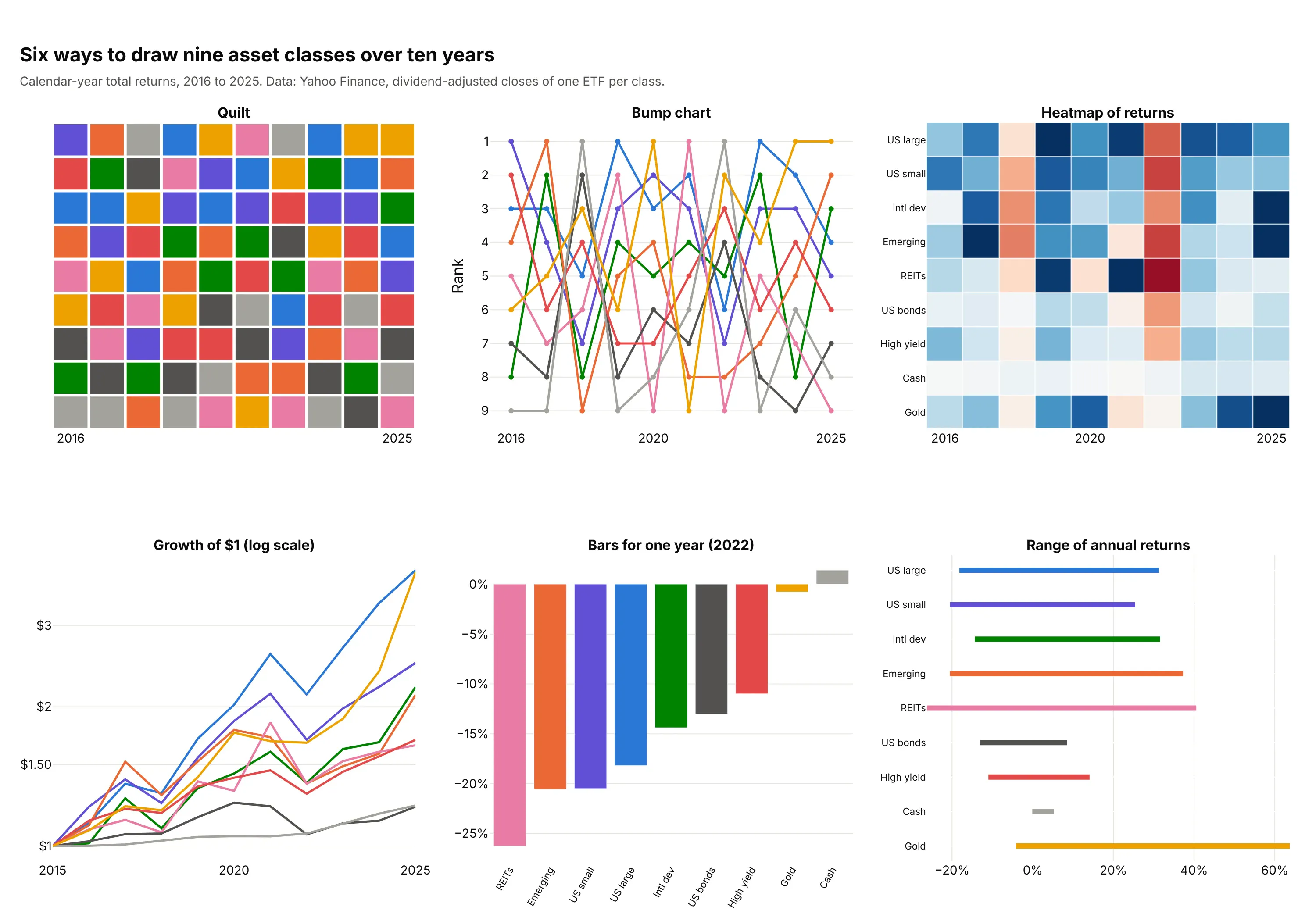
- Periodic table of returns (the chart itself). It answers "which class led each year, and where did it land the year after?" at a glance. It hides the size of the gaps between cells and needs the class names in the cells.
- Bump chart (works too, better for following a few classes). Lines connect each class's rank from year to year, so one class's path is easy to follow, but nine crossing lines are hard to read at once, and the cells' returns are gone.
- Heatmap of returns (different). Color shows the size of each return, so it reveals magnitude, such as gold's 63.7% in 2025, that the quilt hides. It doesn't show rank order.
- Line chart of the growth of $1 (different). It shows what each class was worth at the end, which is what an investor ends up with, but not the year-by-year ordering. Use a log scale so that equal percentage moves look equal.
- Bar chart for one year (worse for history). A sorted bar chart is the best way to show one year, and it is one column of the quilt, but ten years need ten bar charts.
- Range chart (different). A dot plot or range of each class's lowest and highest year shows how risky each class was, which the quilt only hints at. A drawdown chart shows the losses from a peak, and an efficient frontier shows the trade-off between return and risk for combinations of classes.
How to make a periodic table of returns
Plotly has no dedicated trace for a quilt. It is built from a heatmap trace in which the class decides each cell's color (fast, with one text color for all cells), or from one rectangle shape and one text annotation per cell (slower, but each cell can have its own text color and an outline).
With AI
ChatGPT, Claude Code, GitHub Copilot, Cursor and other AI tools are excellent at writing Plotly code. Name Plotly in the prompt, and say how to rank the classes, how to color them and which years to include:
Make a plotly periodic table of returns (quilt chart) from returns.csv (columns: year, asset_class, total_return_pct).- One column per calendar year; in each column rank the asset classes from the best return (top row) to the worst.- Use a go.Heatmap whose z is the class index plus 0.5 and a stepped colorscale, so every class keeps one fixed colorin every year; show the class name and the return with texttemplate, with the year labels on top.- Round returns to one decimal place with a % sign, leave a small gap between cells, and add a hover label with theyear, the class, the return and the rank.- Check: print the first-place class of each year and the last-place class of each year.
With Plotly Studio
Plotly Studio is a product for creating data visualizations and Dash apps and for analyzing data with AI, available as a desktop app or embedded in Dash apps. Ask for a periodic table of returns the same way:
Show a periodic table of returns of the asset classes in this file: one column per year, classes ranked best to worst in each year, each class in one fixed color, the class name and its return in every cell, a year range slider, and a dropdown to outline one class.
Make a periodic table of returns in Python or JavaScript
This is the code AI tools write under the hood. The helper below ranks the classes in each year and draws a heatmap in which the class index, not the return, picks the color; the return only goes into the text. The prices come from the yfinance package, which reads Yahoo Finance and returns dividend-adjusted closes (total returns) by default:
import pandas as pdimport plotly.graph_objects as goimport yfinance as yfdef make_quilt(returns, colors, fmt="{:+.1f}%"):"""returns: DataFrame of percent returns (index = years, columns = asset classes).colors: {class: color}. One column per year, the best class on top, one fixed color per class."""classes = list(returns.columns)n = len(classes)ranked = {y: returns.loc[y].sort_values(ascending=False) for y in returns.index}z = [[classes.index(ranked[y].index[r]) + 0.5 for y in returns.index] for r in range(n)] # the class picks the colortext = [[f"<b>{ranked[y].index[r]}</b><br>{fmt.format(ranked[y].iloc[r])}" for y in returns.index] for r in range(n)]scale = [s for i, c in enumerate(classes) for s in ([i / n, colors[c]], [(i + 1) / n, colors[c]])] # steppedfig = go.Figure(go.Heatmap(z=z, x=[str(y) for y in returns.index], text=text, texttemplate="%{text}",colorscale=scale, zmin=0, zmax=n, showscale=False, xgap=3, ygap=3,hoverinfo="text", textfont=dict(color="white", size=13)))fig.update_yaxes(autorange="reversed", showticklabels=False, ticks="")fig.update_xaxes(side="top")return figfunds = {"SPY": "US large", "AGG": "US bonds", "VNQ": "REITs", "GLD": "Gold", "BIL": "Cash"}colors = {"US large": "#2a78d6", "US bonds": "#52514e", "REITs": "#c4467a", "Gold": "#b07a00", "Cash": "#6f6e68"}prices = yf.download(list(funds), start="2020-12-01", end="2026-01-01", auto_adjust=True, progress=False)["Close"]year_end = prices.resample("YE").last() # last trading day of each calendar yearreturns = (year_end.pct_change().dropna() * 100).rename(columns=funds)returns.index = returns.index.yearmake_quilt(returns, colors).update_layout(width=760, height=520).show()
This draws the five classes for 2021 to 2025, with gold first in 2024 and 2025 (26.7% and 63.7%). Any CSV of annual returns by class works the same way: read it into a DataFrame with years as the index and classes as columns, and pass it to make_quilt. The fmt argument sets the label, so "{:+.0f}" drops the decimals. The white label text needs mid-dark colors; for light cells like pastel pink, use the shapes version below instead, which lets each cell choose its text color.
In JavaScript, plotly.js draws the same chart; the ranking is one sort per year:
<div id="chart"></div><script src="https://cdn.plot.ly/plotly-4.1.1.min.js"></script><script>// Calendar-year total returns in percent (Yahoo Finance, dividend-adjusted closes), 2021 to 2025const years = ["2021", "2022", "2023", "2024", "2025"];const returns = {"US large": [28.7, -18.2, 26.2, 24.9, 17.7],"US bonds": [-1.8, -13.0, 5.7, 1.3, 7.2],"REITs": [40.5, -26.3, 11.9, 4.8, 3.2],"Gold": [-4.1, -0.8, 12.7, 26.7, 63.7],"Cash": [-0.1, 1.4, 4.9, 5.2, 4.1],};const colors = {"US large": "#2a78d6", "US bonds": "#52514e", "REITs": "#c4467a", "Gold": "#b07a00", "Cash": "#6f6e68"};const names = Object.keys(returns), n = names.length;// For each year, order the classes from best to worst: row 0 is the bestconst z = [], text = [];for (let r = 0; r < n; r++) { z.push([]); text.push([]); }years.forEach((y, j) => {const order = names.slice().sort((a, b) => returns[b][j] - returns[a][j]);order.forEach((c, r) => {z[r].push(names.indexOf(c) + 0.5); // the class decides the colortext[r].push(`<b>${c}</b><br>${returns[c][j].toFixed(1)}%`);});});// A stepped colorscale: each class owns one band of 0 to nconst scale = names.flatMap((c, i) => [[i / n, colors[c]], [(i + 1) / n, colors[c]]]);Plotly.newPlot("chart", [{type: "heatmap", z, x: years, text, texttemplate: "%{text}", colorscale: scale, zmin: 0, zmax: n,showscale: false, xgap: 3, ygap: 3, hoverinfo: "text", textfont: {color: "white", size: 14}}], {width: 760, height: 520, yaxis: {autorange: "reversed", showticklabels: false, ticks: ""},xaxis: {side: "top"}, margin: {l: 20, r: 20, t: 50, b: 20}});</script>
For per-cell text colors, an outline around one class or a key, draw each cell as a layout.shapes rectangle and each label as a layout.annotations entry, as the images in this guide do. That is slower for large tables (see the FAQ).
Share it
Every Plotly chart has a Share chart button (the cloud icon in its toolbar) that uploads it to Plotly Cloud and gives you a link. Only you can see it until you change its visibility.
For a live app, put the chart in a Dash app and publish it with the Plotly Cloud CLI. Coding agents can run these commands for you:
pip install "dash[cloud]"plotly user loginplotly app publish
If your data has to stay in your own cloud or data center, publish to Dash Enterprise instead.
Dos and don'ts
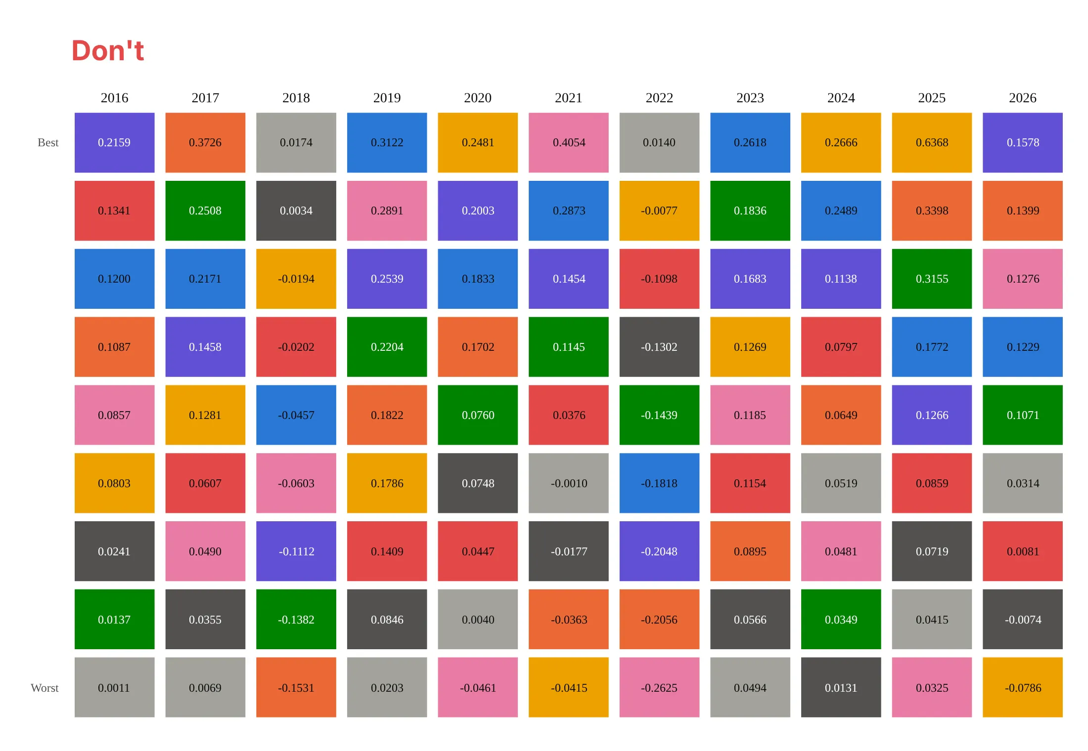
Most mistakes in published quilts make the classes hard to follow or the numbers hard to trust: colors with no names, raw decimals, a year that is not over, or a default font. Here is the main example both ways, in the same colors.
Don't leave the class names out of the cells and drop the key, so that readers must match colors by memory, print raw decimals (0.2159) instead of rounded percents, add the current year before it is over without marking it as partial, or keep a serif default font:
Do put the class name and the rounded return with a percent sign in every cell, rank each year from best to worst, show full calendar years only, and use one clean sans-serif font:
Checklist
Do
- Use calendar-year total returns, and say so, with the source and the start and end dates.
- Keep the same classes, in the same colors, in every column, and name them in every cell.
- Rank each column from best (top) to worst (bottom), and put the year labels on top.
- Show full years only, or mark a partial year clearly.
- Round returns to one decimal place and say whether they are before or after fees.
- Pick classes that don't overlap (large-cap and small-cap stocks, not three large-cap funds).
Don't
- Reassign colors by rank or by return: the point is following one class.
- Use more than about ten classes; the colors blur and the cells shrink.
- Read a future prediction into the order: the table describes the past (see example 10).
- Compare tables with different classes, indices or fee treatment as if they were the same.
More periodic table examples
Six more periodic tables from real public data, each with its source, the technique that makes it work and a prompt to rebuild it. They cover bonds, countries, health care funds, a measure that is not a return, and two tests of what the table shows.
1. Nine bond funds: when every cell is negative
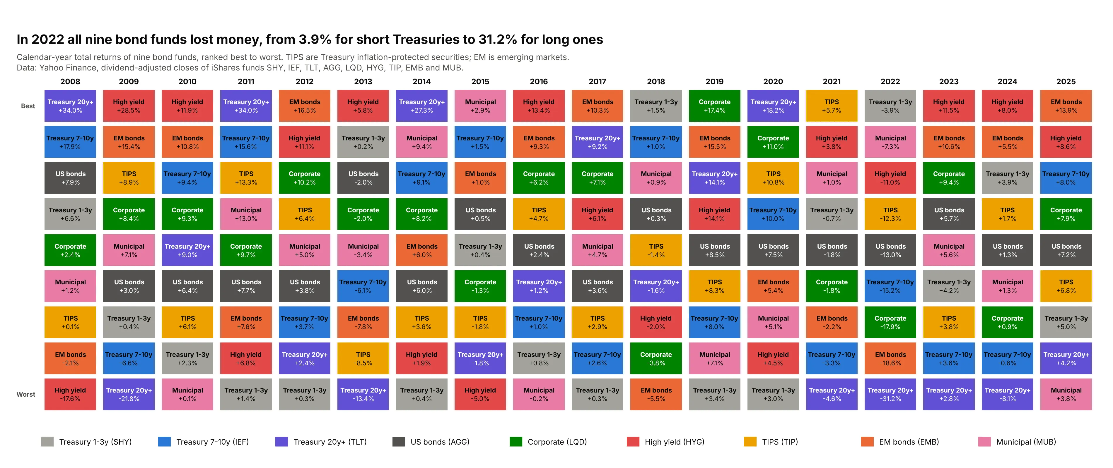
In 2022 all nine bond funds lost money, from 3.9% for 1-3 year Treasuries to 31.2% for 20+ year Treasuries, because long bonds lose the most when interest rates rise. The same 20+ year Treasuries finished first in 2008, 2011, 2014 and 2020, with gains of 34.0%, 34.0%, 27.3% and 18.2%. Data: Yahoo Finance, dividend-adjusted closes of the iShares funds SHY, IEF, TLT, AGG, LQD, HYG, TIP, EMB and MUB, 2008 to 2025.
Tip: when a whole column is negative, the ranking still works, so keep the order and label the returns instead of changing the color scale.
Get the data from Yahoo Finance (dividend-adjusted closes of the iShares bond funds SHY, IEF, TLT, AGG, LQD, HYG, TIP,EMB and MUB, month-end, December 2007 to December 2025) and shape it into a table (columns: year, fund,total_return_pct) using the last trading day of each December.Build a plotly periodic table of returns: one column per year, funds ranked best to worst, a fixed color per fund,the fund name and return in every cell, and a title that states how many funds lost money in 2022.
2. Ten country stock markets
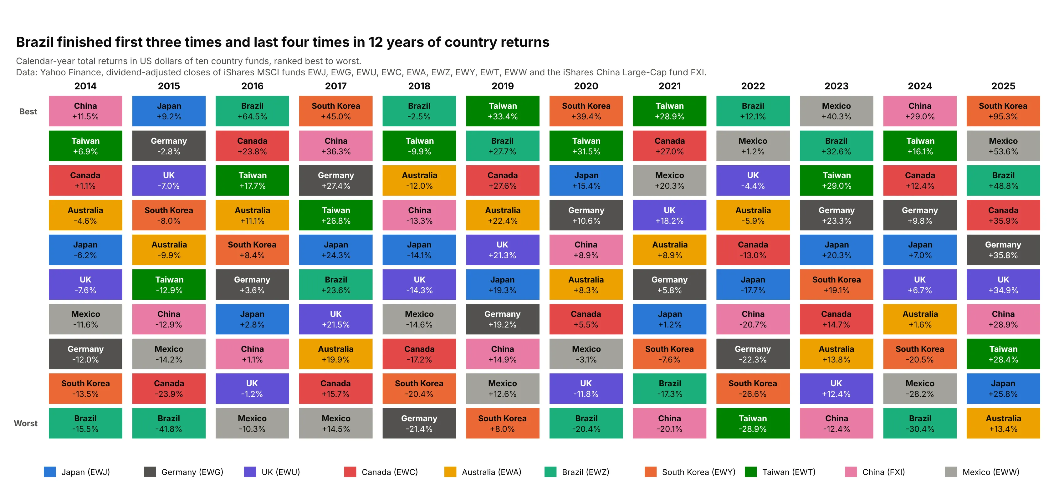
Six different countries finished first in 12 years, and Brazil finished first three times and last four times. In 2025 the range ran from South Korea at 95.3% to Australia at 13.4%, in US dollars, so currency moves are part of each result. Data: Yahoo Finance, dividend-adjusted closes of the iShares MSCI single-country funds EWJ, EWG, EWU, EWC, EWA, EWZ, EWY, EWT and EWW and the iShares China Large-Cap fund FXI, 2014 to 2025.
Tip: say which currency the returns are in, because a country fund in US dollars mixes the stock market with the exchange rate.
Get the data from Yahoo Finance (dividend-adjusted closes of the iShares MSCI country funds EWJ, EWG, EWU, EWC, EWA,EWZ, EWY, EWT and EWW and the iShares China Large-Cap fund FXI, December 2013 to December 2025) and shape it into atable (columns: year, country, total_return_pct).Build a plotly periodic table of returns with one column per year, countries ranked best to worst, one fixed colorper country, and the country name and return in every cell; state in the subtitle that returns are in US dollars.
3. Six health care funds
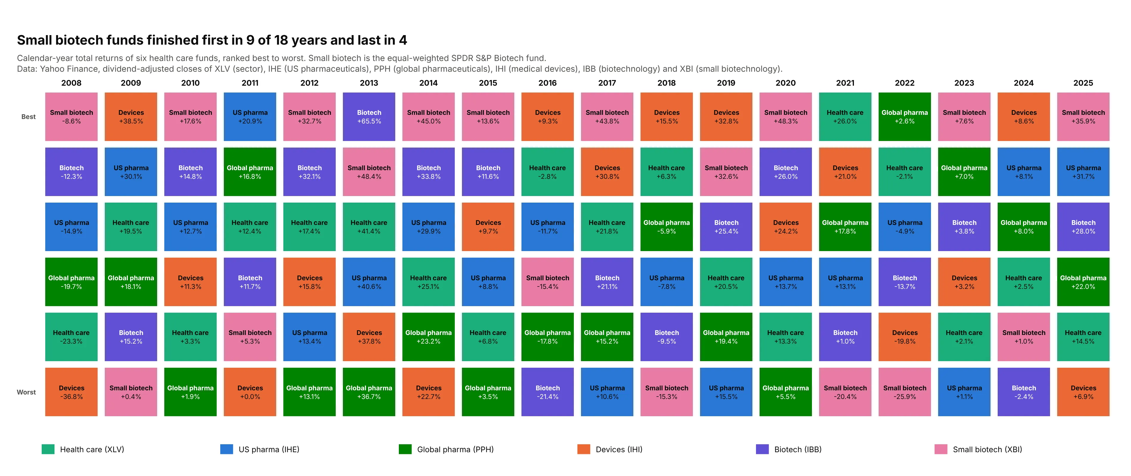
The equal-weighted biotechnology fund finished first in 9 of 18 years and last in four, for example +48.4% in 2013 and -25.9% in 2022, while the broad health care sector fund finished first only once, in 2021. Data: Yahoo Finance, dividend-adjusted closes of XLV (health care sector), IHE (US pharmaceuticals), PPH (global pharmaceuticals), IHI (medical devices), IBB (biotechnology) and XBI (equal-weighted biotechnology), 2008 to 2025.
Tip: with only six classes, make the cells wider and the text larger so the table stays readable on a phone.
Get the data from Yahoo Finance (dividend-adjusted closes of the health care funds XLV, IHE, PPH, IHI, IBB and XBI,month-end, December 2007 to December 2025) and shape it into a table (columns: year, fund, total_return_pct).Build a plotly periodic table of returns with six rows ranked best to worst per year, a fixed color per fund, thefund name and return in every cell, and a title with how often the biotech fund finished first and last.
4. A table of something that is not a return
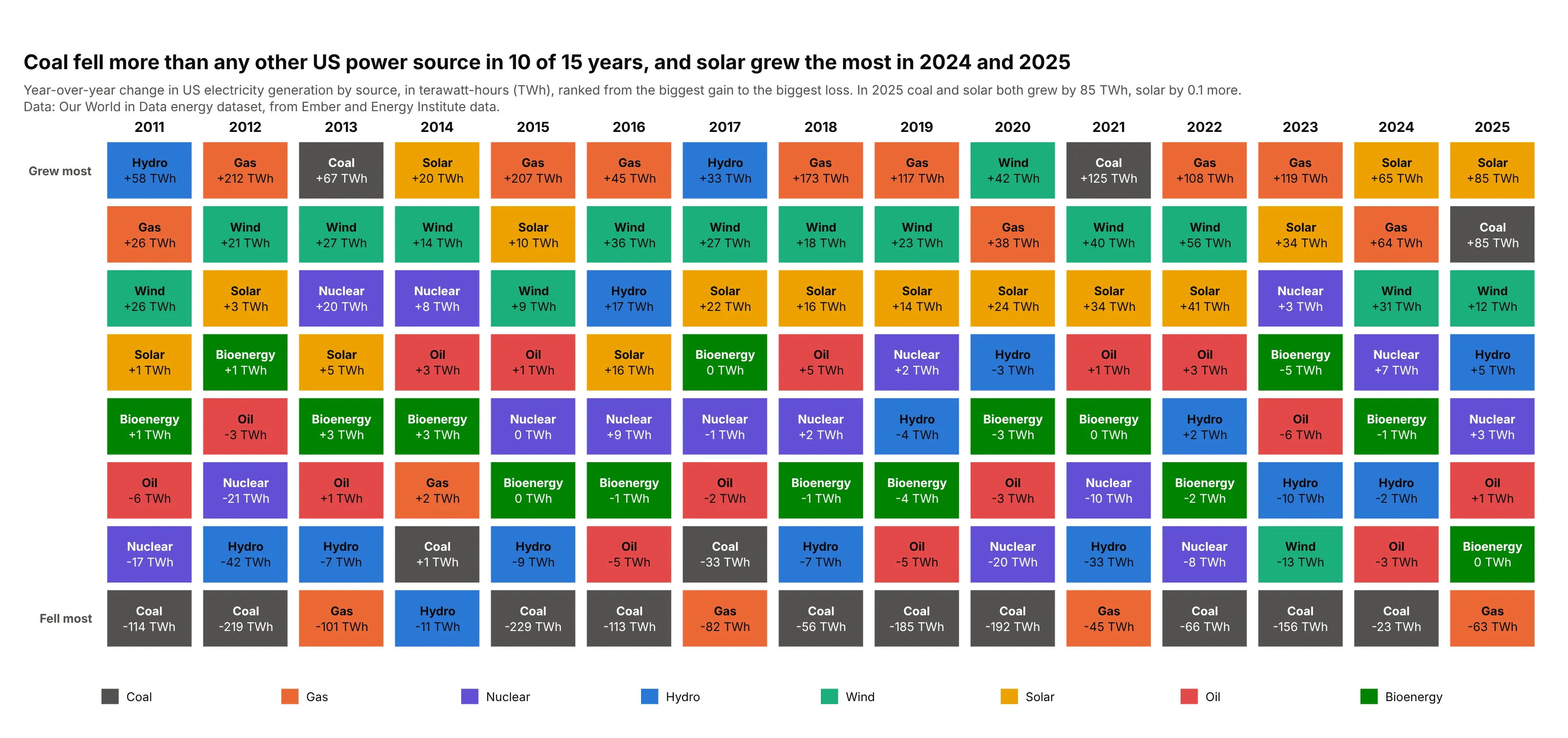
The cell does not have to be a return. Here it is the yearly change in US electricity generation, in terawatt-hours (TWh), so the top of each column is the source that grew most. Coal fell more than any other source in 10 of 15 years, gas grew the most in seven, and solar grew the most in 2014, 2024 and 2025: in 2025 solar added 85 TWh, and coal added 85 TWh too (solar by 0.1 TWh more). Data: Our World in Data energy dataset, built from Ember and Energy Institute data, 2010 to 2025.
Tip: change the first and last row labels ("Grew most", "Fell most") to fit the measure.
Get the data from the Our World in Data energy dataset (owid-energy-data.csv, country "United States", columnscoal_electricity, gas_electricity, nuclear_electricity, hydro_electricity, wind_electricity, solar_electricity,oil_electricity and biofuel_electricity, in terawatt-hours, 2010 to 2025) and shape it into a table (columns: year,source, change_twh) with the change from the previous year.Build a plotly periodic table with one column per year from 2011, sources ranked from the biggest gain to thebiggest loss, a fixed color per source, and the source name and change in TWh in every cell.
5. Zooming out to five years
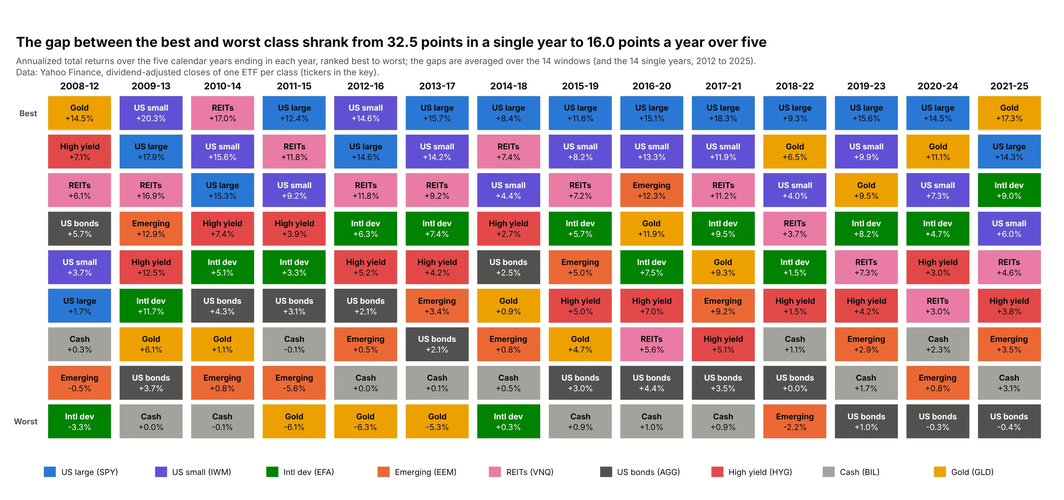
Over rolling five-year windows the table looks calmer: the average gap between the best and worst class was 16.0 percentage points a year, against 32.5 points in the single years of 2012 to 2025, and the S&P 500 finished first in nine of the 14 windows. Data: Yahoo Finance, annualized total returns of the nine ETFs of the first example, windows ending 2012 to 2025.
Tip: annualize the five-year return with the geometric mean, (product of (1 + yearly return)) ** (1 / 5) - 1, not the simple average of the five years.
Get the data from Yahoo Finance (dividend-adjusted closes of SPY, IWM, EFA, EEM, VNQ, AGG, HYG, BIL and GLD,month-end, December 2007 to December 2025) and shape it into calendar-year returns, then into the annualized returnof every five-year window ending 2012 to 2025 (columns: window_end_year, fund, annualized_return_pct).Build a plotly periodic table with one column per window labeled like "2021-25", funds ranked best to worst, onefixed color per fund, and the average best-to-worst gap in the title.
6. Does last year's rank predict this year's?
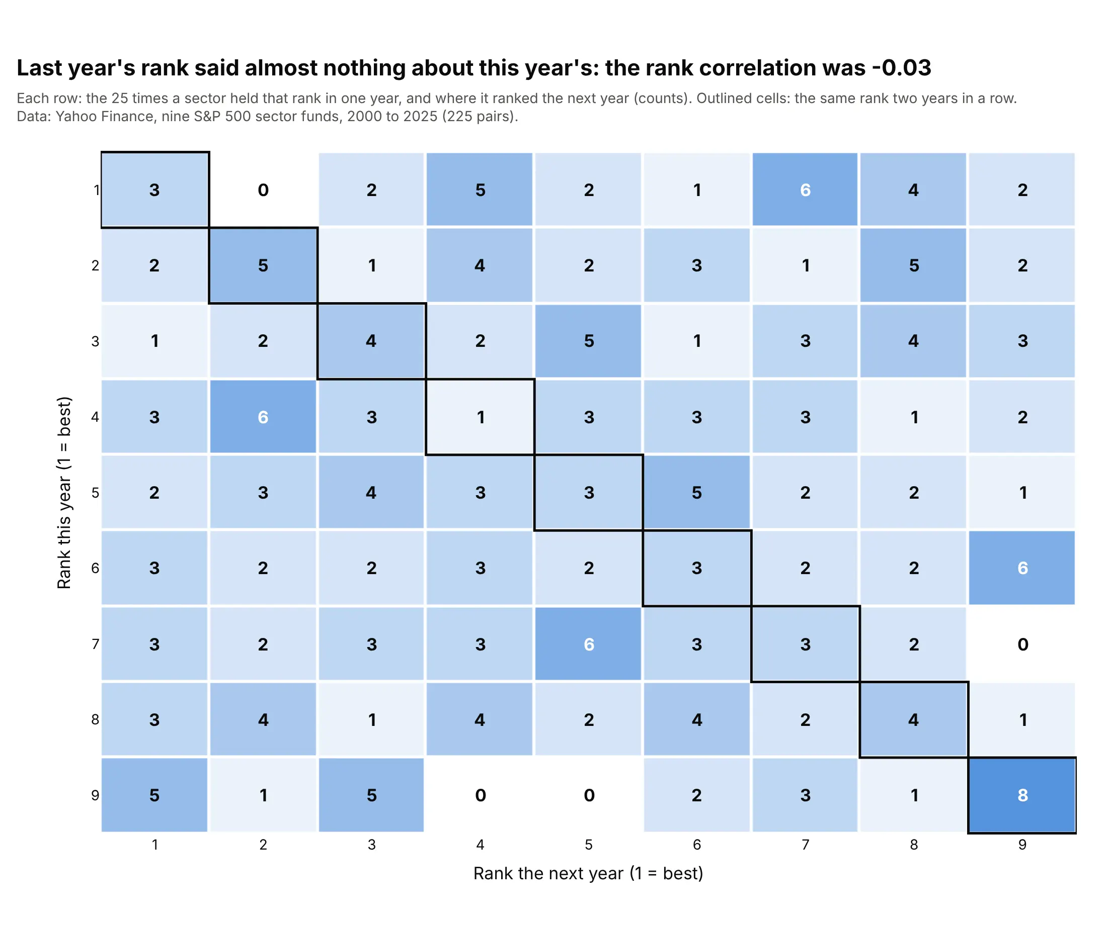
Counting what happens after each rank turns the table into a test. Across 225 pairs of years for the nine S&P 500 sectors (2000 to 2025), the rank correlation from one year to the next was -0.03. The first-place sector stayed first only three times in 25 and fell into the bottom three 12 times (chance would give about eight), while the last-place sector stayed last eight times (chance gives about three) and moved to first five times, so the effects pull in different directions. Data: Yahoo Finance, the nine Select Sector SPDR funds, 2000 to 2025.
Tip: to read a transition table, compare each cell with the count you would get by chance, which is 25 divided by 9, about three.
Get the data from Yahoo Finance (dividend-adjusted closes of the nine Select Sector SPDR funds XLB, XLE, XLF, XLI,XLK, XLP, XLU, XLV and XLY, month-end, December 1999 to December 2025) and shape it into calendar-year returns, theninto each sector's rank (1 = best) in every year (columns: year, sector, rank).Pair each sector's rank in one year with its rank the next year, count the pairs in a 9 by 9 table, and build aplotly heatmap with the count in each cell, the diagonal outlined, and the rank correlation in the title.
FAQ
Options to customize
A periodic table of returns in Plotly is a go.Heatmap with a stepped colorscale, or a set of layout.shapes and layout.annotations, so these are the options that matter most. The full lists are in the heatmap trace reference, the heatmap documentation, the shapes documentation and the text and annotations documentation.
- colorscale with zmin and zmax: a stepped scale, two stops at the same color per class ([i/n, color], [(i+1)/n, color]), with zmin=0 and zmax=n so that each integer in z lands in one band.
- z: the class index plus 0.5 for each cell, so the class and not the return decides the color.
- texttemplate="%{text}" with text: the class name and return written in each cell, in HTML such as <b>Gold</b><br>+63.7%.
- textfont: one font size and color for all cells; use shapes and annotations when cells need different colors.
- xgap and ygap: the white gap between cells, in pixels.
- xaxis.side="top": the years on top, as in the field's tables.
- yaxis.autorange="reversed" and showticklabels=False: the best class in the top row, without row numbers.
- hoverinfo="text": hover labels that show the year, class, return and rank instead of the integer in z.
- showscale=False: no colorbar, since the colors are categories; add a key with annotations or dummy go.Scatter traces.
- layout.shapes (type="rect", fillcolor, line): one rectangle per cell, with an outline (line.width=3.5) to follow one class or a portfolio.
- layout.annotations with font.color: one label per cell, with black or white text for each fill.
- title.subtitle: a muted line under the takeaway title for the data source and the return definition.