Chris Parmer

November 12, 2026

Drawdown Charts - A Complete Guide

TL;DR

A drawdown chart shows, for every date, how far an investment sits below the highest value it had reached so far (its running peak), in percent. It is 0% at every new high and negative in between, and the filled area below zero shows how deep each decline went and how long it took to recover.
Drawdown charts are also known as underwater charts, underwater plots and drawdown curves, and are similar to area charts and line charts of the same returns.
The field's conventions: percent below the running peak on the y axis, a filled area down from a zero line, the maximum drawdown labeled with its peak, trough and recovery dates, and the equity curve (the growth of $1, on a log scale) above it on a shared x axis. Portfolio managers and risk teams read it next to the efficient frontier because it shows the losses that volatility summarizes.
You can make a drawdown chart with Plotly in two lines of pandas, price / price.cummax() - 1, and a go.Scatter trace with fill="tozeroy". This guide is educational and is not investment advice.

What is a drawdown chart?

Drawdown charts look like this:

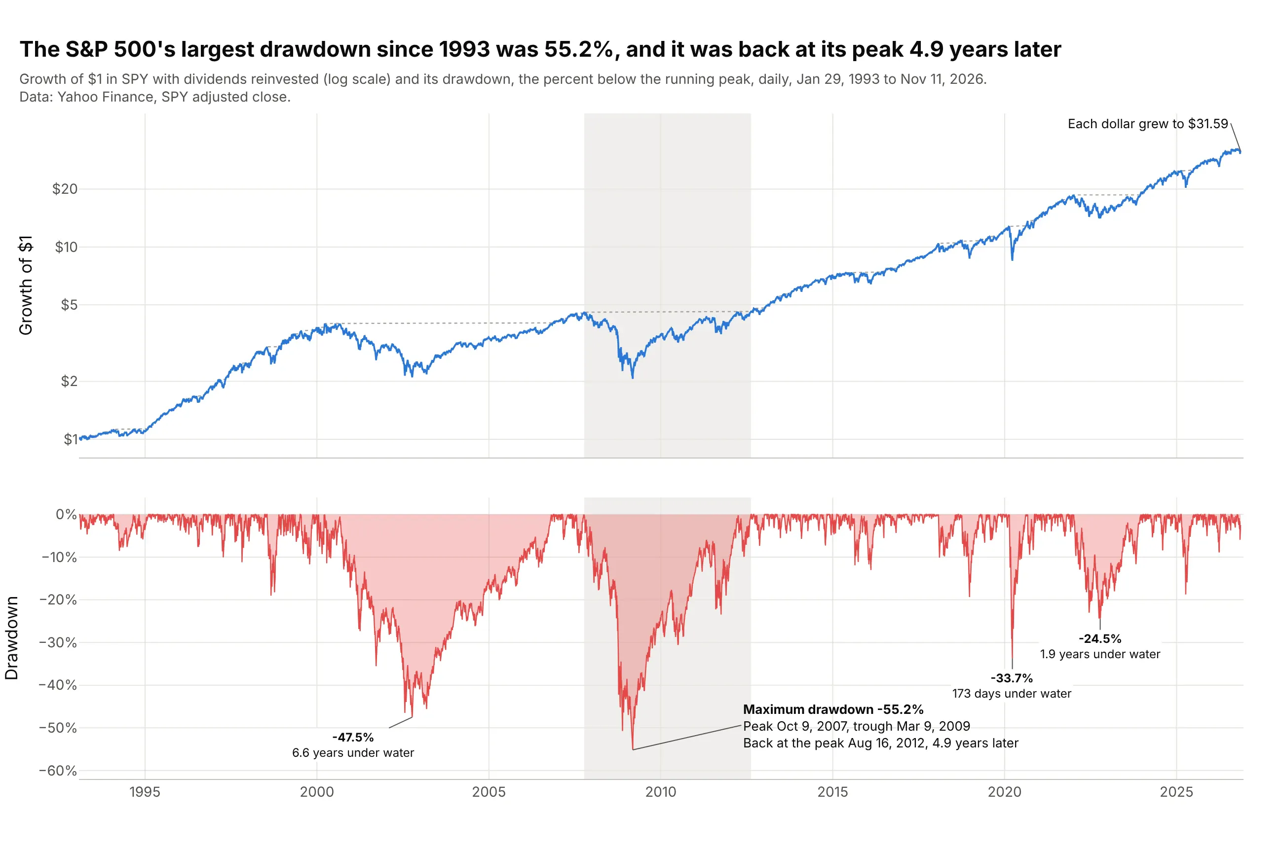
Two panels on a shared time axis, January 1993 to November 2026: on top, the growth of $1 in SPY on a log scale rising to $31.59, with a dotted running peak; below, the drawdown as a red area under a zero line, with the largest episode shaded: 55.2% from the October 9, 2007 peak to the March 9, 2009 trough, back at the peak on August 16, 2012, 4.9 years later; the 2000 episode is labeled 47.5% and 6.6 years under water, 2020 is 33.7% and 173 days, and 2022 is 24.5% and 1.9 years

Data: Yahoo Finance, daily adjusted closes of SPY (the oldest S&P 500 exchange-traded fund, with dividends reinvested), January 29, 1993 to November 11, 2026.

How do you read a drawdown chart? In the example above, notice these things:

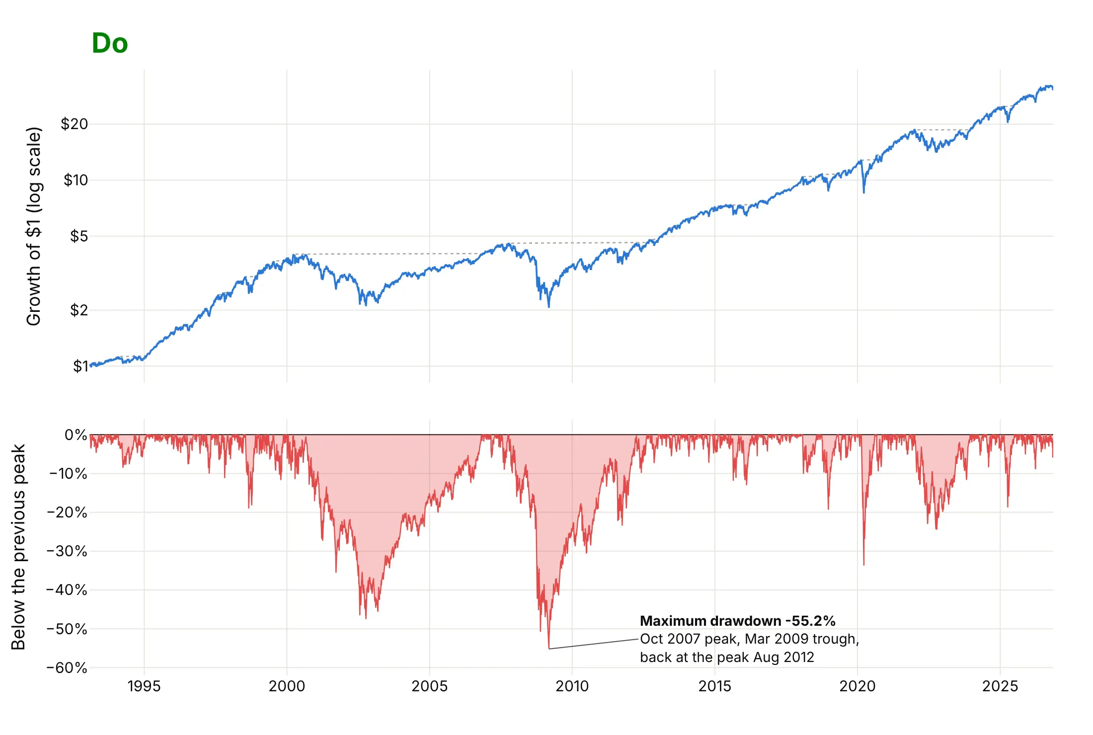
The top panel is the equity curve: what $1 invested in January 1993 was worth on each day, on a log scale so that equal percentage moves look equal. The dotted line is its running peak, the highest value so far, and $1 grew to $31.59.
The bottom panel is the drawdown: the gap between the two lines in percent, computed as value / running peak - 1. It touches 0% on the 10.5% of days that set a new high and is negative on all the others.
The deepest point is the maximum drawdown, 55.2% on March 9, 2009, measured from the peak of October 9, 2007. The fund took 517 days to fall from peak to trough and 1,256 more to get back, 4.9 years in all, which the shaded band marks.
The width of each red area is its duration. The 2000 episode was shallower (47.5%) but lasted longer, 6.6 years, while the 2020 episode fell 33.7% and was back at its peak 173 days after it began.

It's often used for charts like these:

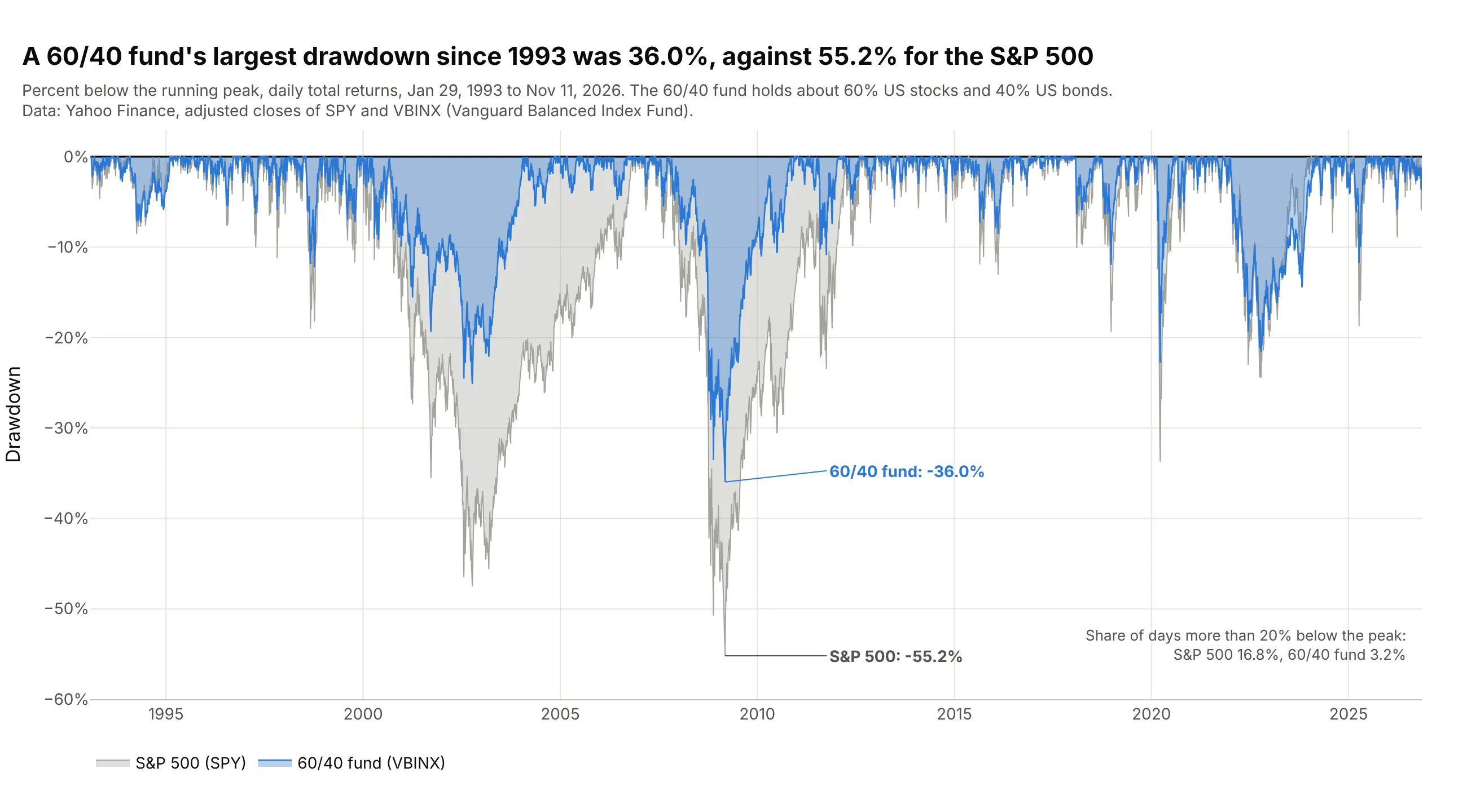
Underwater chart of a 60/40 balanced fund in blue over the S&P 500 in gray, 1993 to 2026: the S&P 500 reaches 55.2% below its peak in March 2009 and the 60/40 fund 36.0%; a note says the S&P 500 spent 16.8% of days more than 20% below its peak and the 60/40 fund 3.2%

Comparing portfolios. Fund fact sheets and portfolio reviews overlay drawdowns to compare how two strategies behaved in the same markets: a fund of about 60% stocks and 40% bonds fell 36.0% at most since 1993, against 55.2% for the S&P 500. Data: Yahoo Finance, SPY and VBINX (Vanguard Balanced Index Fund).

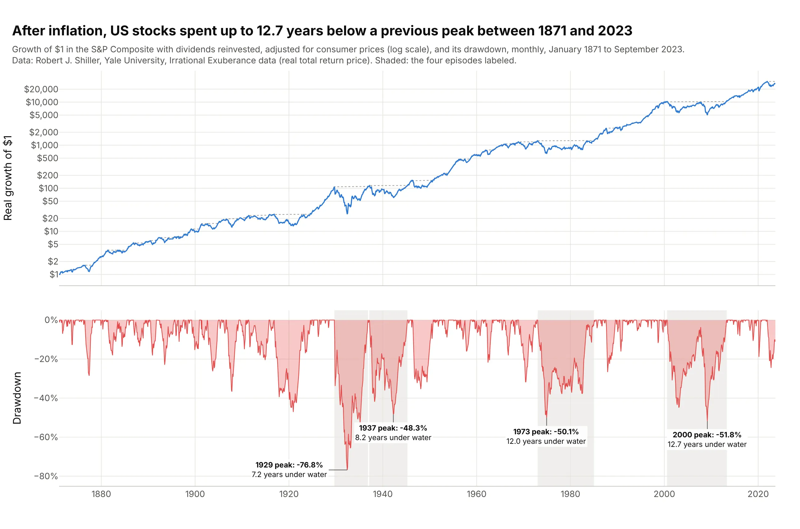
Growth of $1 in US stocks after inflation from 1871 to 2023 on a log scale, and its drawdown below with four shaded episodes: the 1929 peak at 76.8% and 7.2 years under water, the 1937 peak at 48.3% and 8.2 years, the 1973 peak at 50.1% and 12.0 years, and the 2000 peak at 51.8% and 12.7 years

Long market history. The classic underwater chart covers a century or more of stock returns. After inflation, US stocks spent up to 12.7 years below a previous peak, from August 2000 to May 2013. Data: Robert J. Shiller, Yale, monthly S&P Composite real total return, 1871 to 2023.

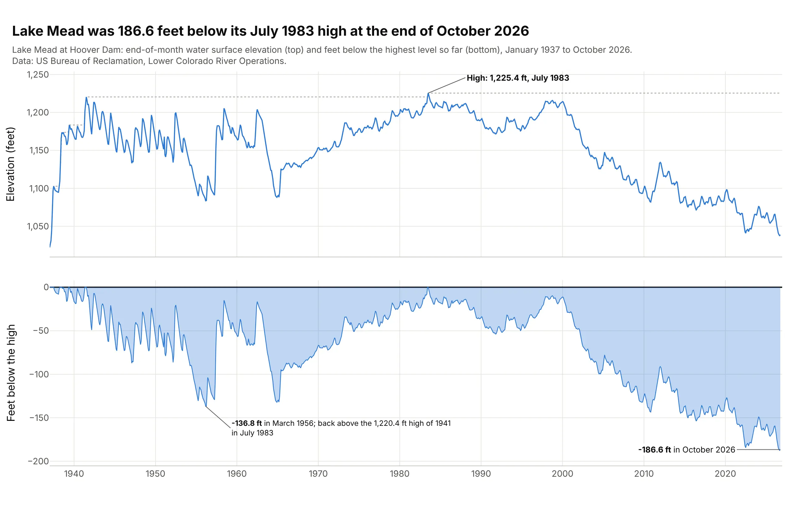
Lake Mead's end-of-month elevation from 1937 to 2026 with its July 1983 high of 1,225.4 feet, and below it the feet below the highest level so far: 136.8 feet in March 1956, refilled above the 1941 high in July 1983, and 186.6 feet in October 2026

Reservoir drawdown in water management. Hydrologists use the same word and the same running-peak calculation for a reservoir's level, in feet rather than percent: Lake Mead was 186.6 feet below its July 1983 high at the end of October 2026. Data: US Bureau of Reclamation, Lake Mead at Hoover Dam, end-of-month elevation.

A short history

Investors have always talked about losses from a high, but the drawdown became a standard risk measure through the managed futures and mutual fund newsletters of the 1980s. Peter Martin developed the Ulcer Index in 1987, the root mean square of the percent drawdowns, and described it with Byron McCann in The Investor's Guide to Fidelity Funds in 1989; his charts of "drawdowns in value" filled the area below each earlier high, as the underwater chart does today (Martin, Ulcer Index page). Terry Young's Calmar ratio of 1991 divided a commodity trading advisor's return by its maximum drawdown (Wikipedia). Academics followed with drawdown-constrained portfolios (Grossman and Zhou 1993), the expected maximum drawdown of a random walk (Magdon-Ismail et al. 2004) and portfolio optimization with drawdown limits (Chekhlov, Uryasev and Zabarankin 2005). In Python, Quantopian's pyfolio and the QuantStats library both draw it under the title "Underwater plot".

Martin's best-known chart made the case against using volatility alone. He took the monthly returns of an S&P 500 index fund from 2000 to 2009 and reordered them, which leaves the volatility and the final value unchanged and changes the drawdown completely. Here is that demonstration redrawn with SPY:

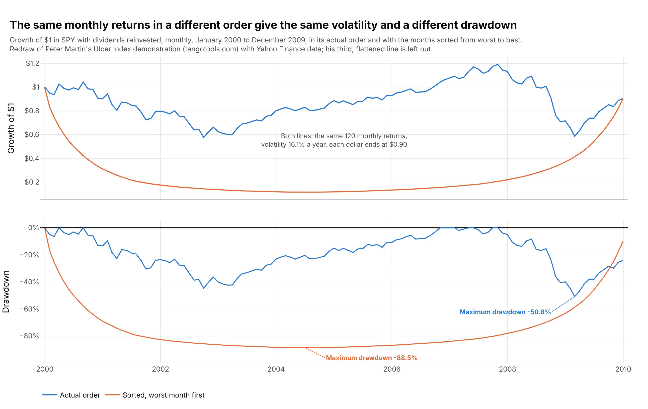
Two panels, 2000 to 2009: the growth of $1 in SPY in its actual monthly order in blue, and the same 120 monthly returns sorted worst first in orange, which falls to about $0.12 before climbing back; both end at $0.90 with volatility of 16.1% a year; in the drawdown panel the actual order reaches 50.8% below its peak and the sorted order 88.5%

Data: Yahoo Finance, SPY month-end adjusted closes, January 2000 to December 2009 (120 monthly returns). A redraw of Peter Martin's demonstration with our data; his third, "flattened" ordering is left out because his shuffling rule isn't given.

How drawdown is calculated

A drawdown chart rests on one running maximum, and most of what people get wrong about it comes from the details around that maximum: which prices go in, how often they are sampled, and how the length of an episode is counted. This section works through them on real data.

The running peak, the trough and the recovery

The running peak at each date is the highest value up to that date, so it only moves up. The drawdown is the value divided by the running peak, minus 1. In early 2020, SPY peaked on February 19, fell to 72.3 on March 23 (on a scale where its December 2, 2019 value is 100), and was back above the old peak on August 10:

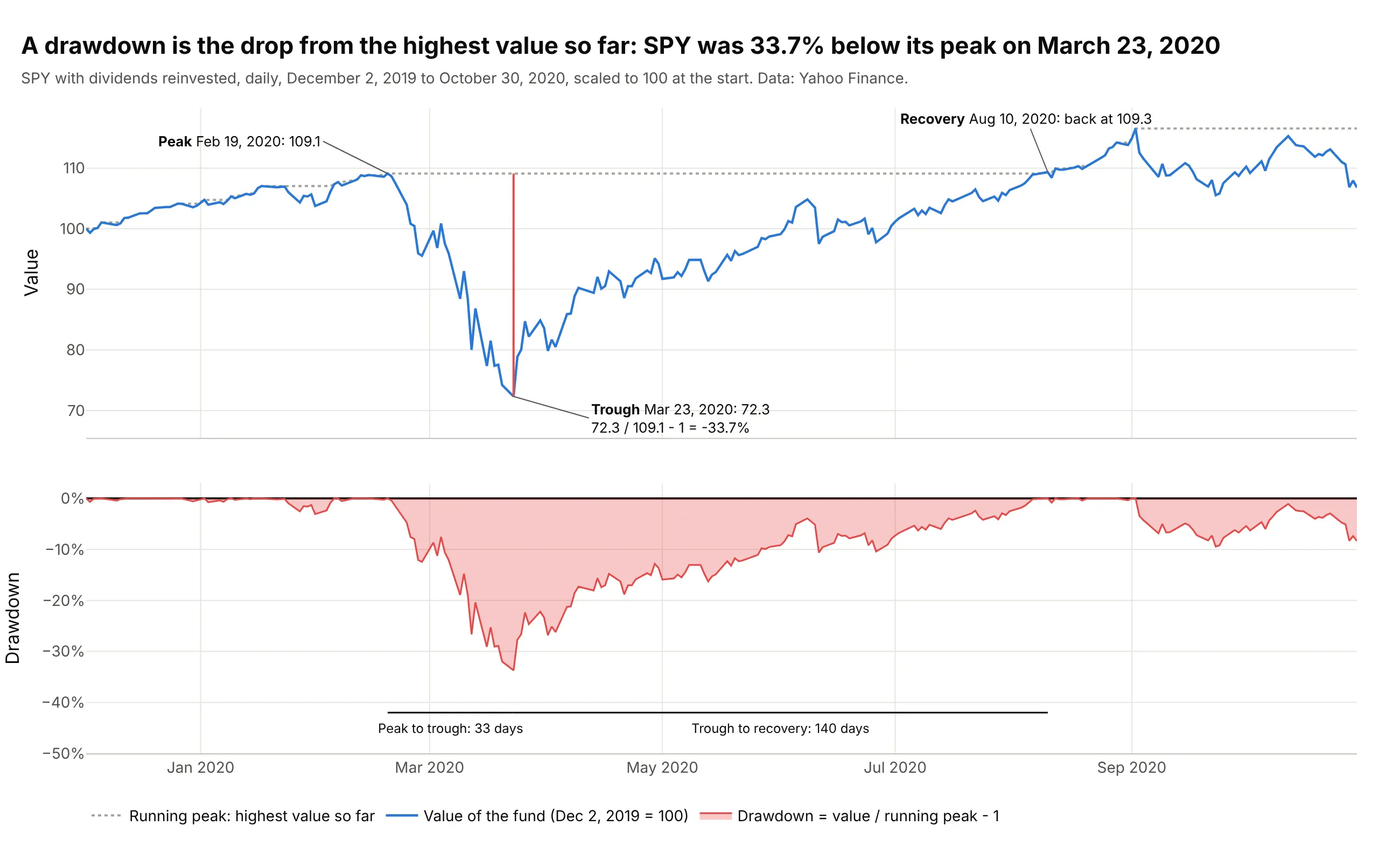
SPY from December 2019 to October 2020 scaled to 100: the fund value with its dotted running peak, a red vertical line from the peak of 109.1 on February 19 down to the trough of 72.3 on March 23, labeled 72.3 / 109.1 - 1 = -33.7%, and the recovery on August 10 at 109.3; below, the drawdown area with brackets for peak to trough, 33 days, and trough to recovery, 140 days

Data: Yahoo Finance, SPY adjusted close.

The words around it have fixed meanings. The maximum drawdown is the deepest point over the whole period, here -33.7%. Peak to trough is the time from the high to that low (33 days), recovery time is the time from the trough back to the old high (140 days), and drawdown duration, or time under water, is the whole span from peak to recovery (173 days). The longest duration doesn't have to belong to the deepest drawdown: in the main example, the 2000 episode lasted 6.6 years and the deeper 2007 one 4.9.

Why a 50% drawdown needs a 100% gain

Losses and gains are not symmetric, because the gain is measured from the lower value. After a drawdown d, getting back to the peak takes a gain of 1 / (1 - d) - 1:

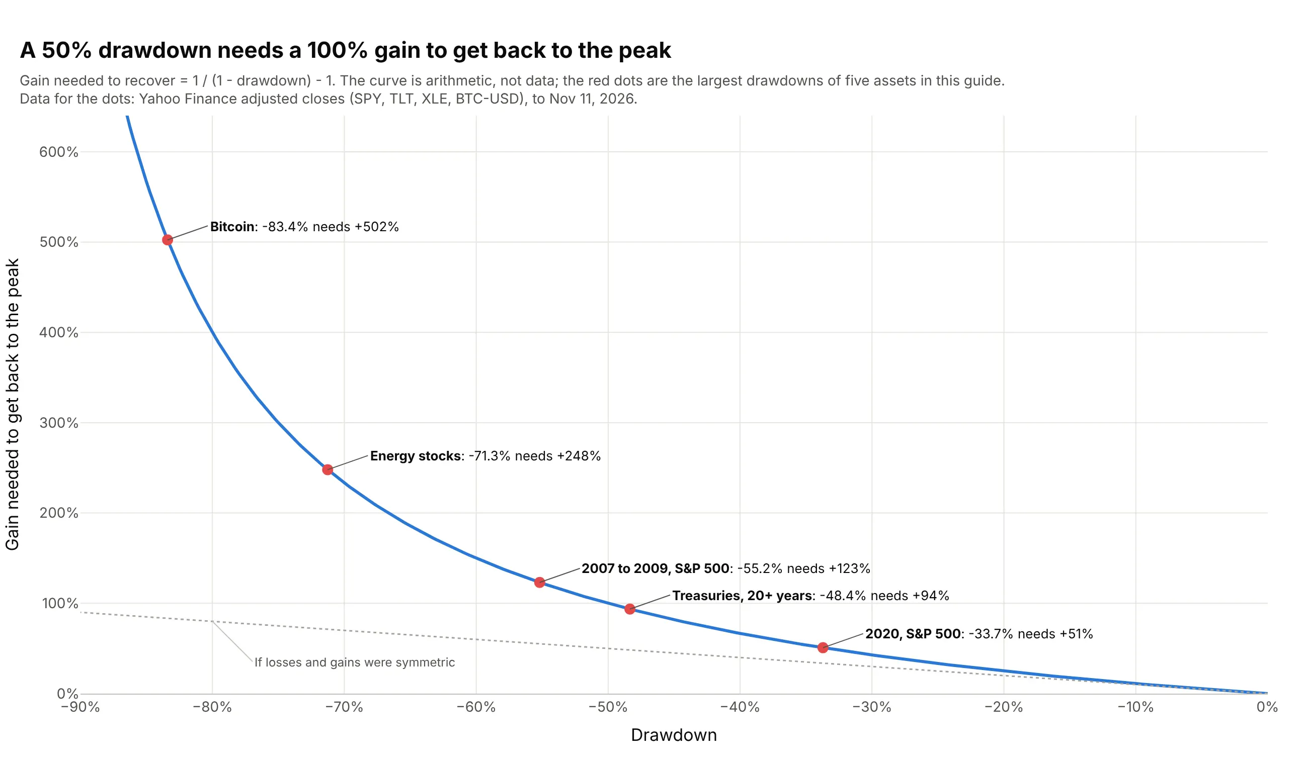
A curve of the gain needed to recover against the drawdown, rising slowly at first and then steeply, with a dotted line for a symmetric loss and gain; red dots mark the S&P 500 in 2020, -33.7% needing +51%, 20+ year Treasuries, -48.4% needing +94%, the S&P 500 in 2007 to 2009, -55.2% needing +123%, energy stocks, -71.3% needing +248%, and bitcoin, -83.4% needing +502%

Data: the curve is arithmetic; the dots are the maximum drawdowns of SPY, TLT, XLE and BTC-USD in this guide (Yahoo Finance).

This is why the underwater area of a deep drawdown is wide: a fund that fell 55.2% had to more than double (+123%) to reach its old high, even though its average daily gain didn't change.

Daily, monthly or yearly data

The maximum drawdown depends on how often you sample the price. A month-end series can step over a fall and recovery that happened inside the month, so it reports a smaller drawdown:

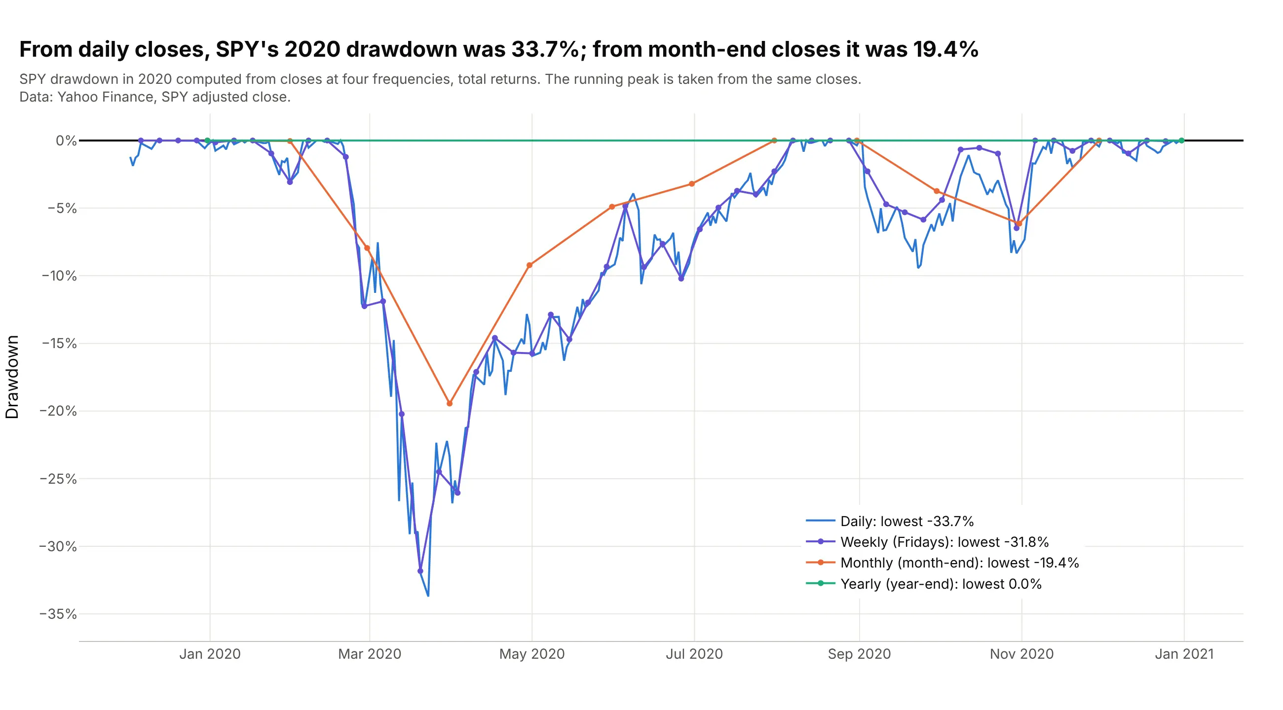
SPY drawdown in 2020 from daily closes in blue (lowest -33.7%), Friday closes in purple (-31.8%), month-end closes in orange (-19.4%) and year-end closes in green (0.0%); the monthly line cuts straight across the March low

Data: Yahoo Finance, SPY adjusted close.

Over the whole 1993 to 2026 history, SPY's maximum drawdown was 55.2% from daily closes, 54.6% from weekly, 50.8% from monthly and 37.5% from yearly closes. Use daily data when you have it and say which frequency you used; Martin recommended weekly or more often for the same reason.

Which prices go in

Use a total return series, with dividends and coupons reinvested, unless you mean to show the price alone: a price index understates the recovery, because dividends keep paying while the price is under water. The S&P 500 price index needed 25.0 years to regain its 1929 high (example 1 below), while Shiller's total return series with dividends, before inflation, took 15.3 years. Adjusting for inflation answers a different question, whether the investor's purchasing power got back to its peak, and makes the episodes longer, as the 1871 chart above shows.

Summary statistics built on drawdowns

Three numbers summarize a drawdown chart. The maximum drawdown is the deepest point; the Calmar ratio divides the annual return by it (SPY: 10.8% / 55.2% = 0.19 over 1993 to 2026, on all the data rather than Young's 36 months); and Martin's Ulcer Index is the square root of the average squared drawdown, which counts depth and duration together (14.4 for SPY and 7.1 for the 60/40 fund). A single maximum is one event and says little about the next one, which is why the full chart is more useful than any of them.

Alternatives to a drawdown chart

Here's the same 33 years of S&P 500 returns drawn six ways. Some are better for the question, some worse, some just different:

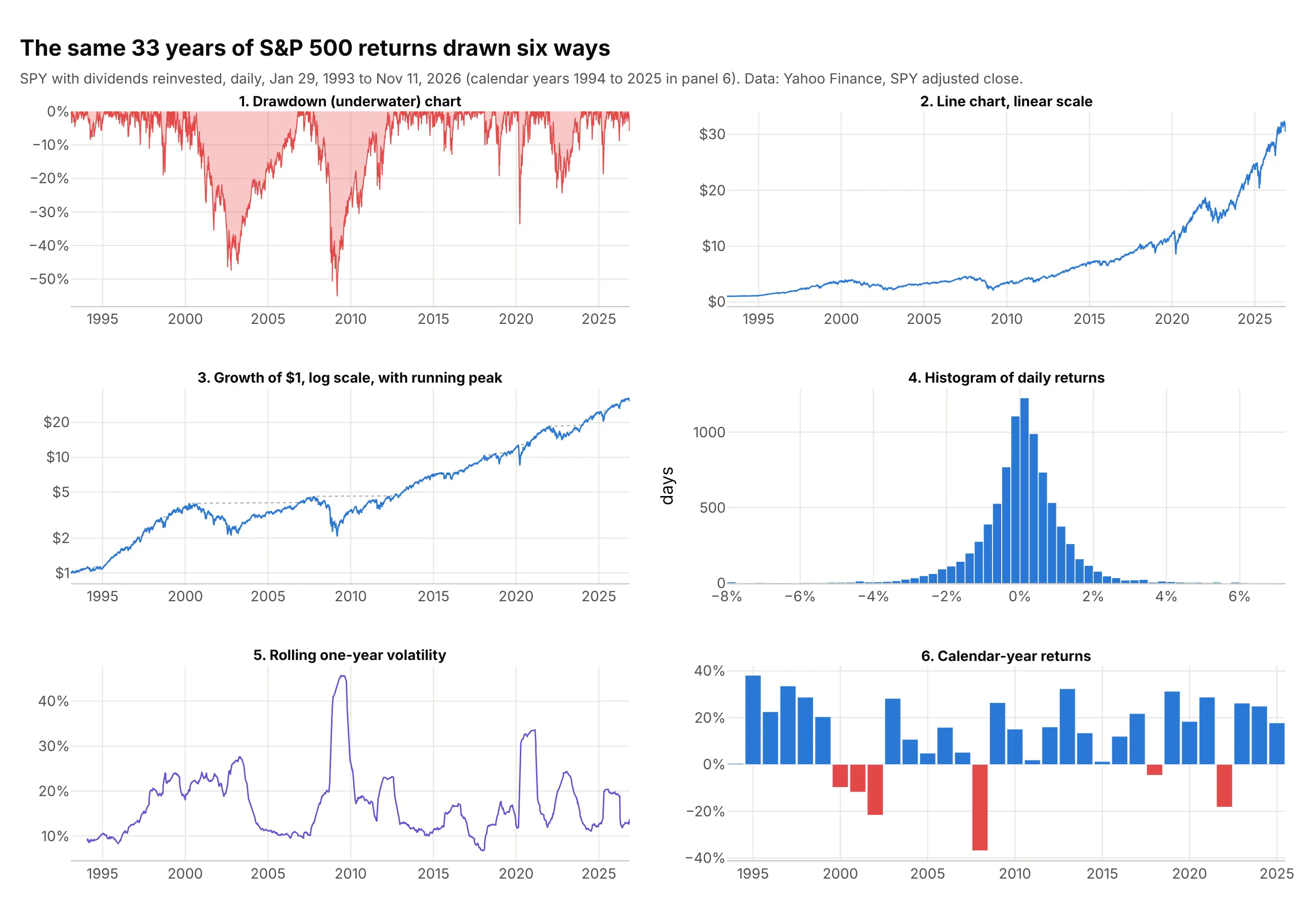
Six small charts of SPY from 1993 to 2026: the underwater chart; the growth of $1 as a line on a linear scale, where everything before 2010 looks flat; the growth of $1 on a log scale with its dotted running peak; a histogram of daily returns centered just above zero; rolling one-year volatility peaking above 40% in 2008 and 2009; and bars of calendar-year returns, with red bars for 2000, 2001, 2002, 2008, 2018 and 2022

Drawdown (underwater) chart (the chart itself). It answers "how much did I lose from the top, and for how long?" for every date, which no other chart shows directly. It hides the level of the investment, so it is usually paired with the equity curve.
Line chart on a linear scale (worse). A rising series makes the early declines look tiny: the 47.5% fall of 2000 to 2002 is a small dent next to recent swings of a few dollars.
Growth of $1 on a log scale with the running peak (works too, and the best companion). Equal percentage moves look equal, and the gap between the line and the dotted peak is the drawdown. Readers find depth harder to read off it, which is why the underwater panel goes below it.
Histogram of daily returns (different). It shows how large single days were, but drawdowns come from runs of losses, and a histogram loses the order. Martin's sorted returns have the same histogram as the real ones.
Rolling volatility (different). A line chart of the standard deviation of returns over the past year shows when markets were turbulent, and it rises for gains as much as for losses.
Bar chart of calendar-year returns (worse for this question). It is easy to read, but calendar years cut episodes in two: 2020 shows a gain even though the fund was 33.7% below its peak in March.

For many assets at once, a scatter of maximum drawdown against annual return (example 7) or small multiples of underwater charts (example 6) work better than one crowded chart.

How to make a drawdown chart

With AI

ChatGPT, Claude Code, GitHub Copilot, Cursor and other AI tools are excellent at writing Plotly code. Name Plotly in the prompt, and say which prices to use and how to mark the maximum drawdown:

Make a plotly drawdown chart from prices.csv (columns: date, adj_close; daily total-return prices).

- Two rows with make_subplots(shared_xaxes=True): growth of $1 on a log y axis with the running peak dotted on top,
  and drawdown = adj_close / adj_close.cummax() - 1 in percent below it, as a red area with fill="tozeroy".
- Find every drawdown episode (peak, trough, recovery date, depth, days peak to trough and trough to recovery) and
  label the deepest one with its dates; shade it from peak to recovery in both panels.
- Percent ticks on the drawdown axis, a zero line, hovermode="x unified", and a title that states the maximum drawdown.
- Check: print the five deepest episodes with their dates and durations.

With Plotly Studio

Plotly Studio is a desktop app where you point an AI at a dataset and it builds charts and a Dash app around your questions. Ask for a drawdown chart the same way:

Show an underwater chart of each fund's drawdown from its running peak, with the growth of $1 above it on a shared time axis, a dropdown to pick the fund, a date range picker that recomputes the peaks, and a table of the five deepest drawdowns with their peak, trough and recovery dates.

Make a drawdown chart in Python or JavaScript

This is the code AI tools write under the hood. pandas computes the drawdown with cummax(), and Plotly draws it as a filled go.Scatter trace below the equity curve. This example reads the S&P 500 from FRED (Federal Reserve Economic Data), which keeps the last 10 years of the index without dividends; on November 11, 2026 it finds a maximum drawdown of 33.9% on March 23, 2020:

import pandas as pd
import plotly.graph_objects as go
from plotly.subplots import make_subplots

# S&P 500 index from FRED (price only, the last 10 years of trading days)
df = pd.read_csv("https://fred.stlouisfed.org/graph/fredgraph.csv?id=SP500", na_values=".",
                 parse_dates=["observation_date"]).dropna()
price = df.set_index("observation_date")["SP500"]

peak = price.cummax()                      # running peak: the highest close so far
drawdown = (price / peak - 1) * 100        # percent below that peak, 0 at every new high
trough = drawdown.idxmin()                 # date of the maximum drawdown

fig = make_subplots(rows=2, cols=1, shared_xaxes=True, row_heights=[0.6, 0.4], vertical_spacing=0.05)
fig.add_scatter(x=price.index, y=price, name="S&P 500", row=1, col=1)
fig.add_scatter(x=peak.index, y=peak, name="Running peak", line=dict(dash="dot", color="gray"), row=1, col=1)
fig.add_scatter(x=drawdown.index, y=drawdown, name="Drawdown", fill="tozeroy",
                line=dict(color="#e34948"), row=2, col=1)
fig.add_annotation(x=trough, y=drawdown.min(), text=f"Max drawdown {drawdown.min():.1f}%",
                   row=2, col=1, ax=60, ay=10)
fig.update_yaxes(type="log", title_text="S&P 500", row=1, col=1)
fig.update_yaxes(ticksuffix="%", title_text="Drawdown", row=2, col=1)
fig.update_layout(hovermode="x unified", showlegend=False)
fig.show()

For a fund or a portfolio, use its total-return prices (adjusted closes) instead, and for returns rather than prices, build the equity curve first with (1 + returns).cumprod(). To list every episode, loop over the dates where drawdown == 0: each run of negative values between two zeros is one episode, with its peak at the first zero and its recovery at the next.

In JavaScript, plotly.js draws the same two panels; the running peak is one Math.max per value:

<div id="chart"></div>
<script src="https://cdn.plot.ly/plotly-4.1.1.min.js"></script>
<script>
  // S&P 500 price index at the end of each quarter, 2006 to 2013 (Yahoo Finance, ^GSPC)
  const dates = ["2006-12-31", "2007-03-31", "2007-06-30", "2007-09-30", "2007-12-31", "2008-03-31", "2008-06-30",
    "2008-09-30", "2008-12-31", "2009-03-31", "2009-06-30", "2009-09-30", "2009-12-31", "2010-03-31", "2010-06-30",
    "2010-09-30", "2010-12-31", "2011-03-31", "2011-06-30", "2011-09-30", "2011-12-31", "2012-03-31", "2012-06-30",
    "2012-09-30", "2012-12-31", "2013-03-31", "2013-06-30", "2013-09-30", "2013-12-31"];
  const close = [1418.30, 1420.86, 1503.35, 1526.75, 1468.36, 1322.70, 1280.00, 1166.36, 903.25, 797.87, 919.32,
    1057.08, 1115.10, 1169.43, 1030.71, 1141.20, 1257.64, 1325.83, 1320.64, 1131.42, 1257.60, 1408.47, 1362.16,
    1440.67, 1426.19, 1569.19, 1606.28, 1681.55, 1848.36];
  let peak = -Infinity;
  const drawdown = close.map(c => { peak = Math.max(peak, c); return (c / peak - 1) * 100; });
  Plotly.newPlot("chart", [
    {x: dates, y: close, mode: "lines", name: "S&P 500", line: {color: "#2a78d6"}},
    {x: dates, y: drawdown, mode: "lines", name: "Drawdown", fill: "tozeroy", xaxis: "x", yaxis: "y2",
     line: {color: "#e34948"}, hovertemplate: "%{y:.1f}% below the peak<extra></extra>"}
  ], {
    width: 900, height: 560, showlegend: false, hovermode: "x unified",
    yaxis: {title: {text: "S&P 500"}, domain: [0.45, 1]},
    yaxis2: {title: {text: "Drawdown"}, ticksuffix: "%", domain: [0, 0.38]}
  });
</script>

Share it

Every Plotly chart has a Share chart button (the cloud icon in its toolbar) that uploads it to Plotly Cloud and gives you a link. Only you can see it until you change its visibility.

For a live app, put the chart in a Dash app and publish it with the Plotly Cloud CLI. Coding agents can run these commands for you:

pip install "dash[cloud]"
plotly user login
plotly app publish

If your data has to stay in your own cloud or data center, publish to Dash Enterprise instead.

Dos and don'ts

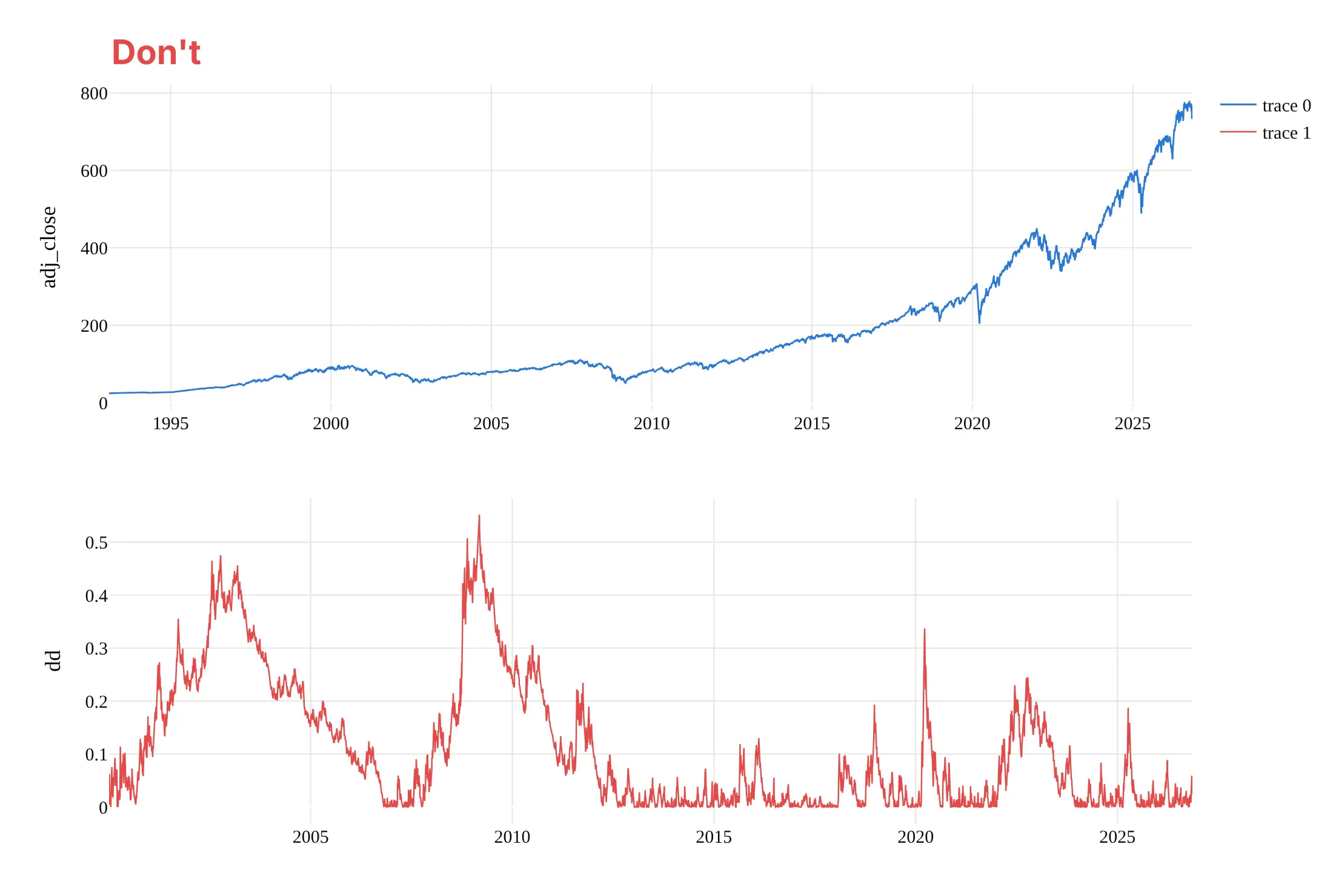
Most mistakes in published drawdown charts make the declines hard to read: drawdowns plotted upward so they look like gains, panels that don't line up in time, or a linear scale that hides the early history. Here is the main example both ways, in the same colors.

Don't plot the drawdown as a positive decimal going up, start the two panels on different dates with separate x axes, put the price on a linear scale, leave raw column names ("adj_close", "dd") and default trace names in a legend, skip the maximum, or keep a serif default font:

Two panels in a serif font: SPY's adjusted close on a linear axis from 0 to 800, where everything before 2010 looks flat, and below it the drawdown as a red line rising upward from 0 to 0.55, starting in 2000 on its own x axis so the years don't line up with the panel above; the axes are titled adj_close and dd, and a legend reads trace 0 and trace 1

Do put the growth of $1 on a log scale above, the drawdown in percent below zero and filled down to it, one shared x axis, and a label on the maximum drawdown with its dates:

The same data with the growth of $1 on a log scale from $1 to about $30 and its dotted running peak, and below it the drawdown as a red area from 0% down to -60% on the same time axis, with the maximum labeled: -55.2%, October 2007 peak, March 2009 trough, back at the peak August 2012, in Inter

Checklist

Use total-return prices (dividends reinvested), and say so; say if the series is inflation-adjusted.
Compute drawdowns from daily data when you have it, and state the frequency.
Keep the drawdown axis at 0% at the top, negative values below, with the same range when you compare assets.
Label the maximum drawdown with its peak, trough and recovery dates, and the time under water.
Show the equity curve (log scale) or the price on a shared x axis, so readers see what the drawdowns are from.

Don't

Start the chart at a convenient low: the running peak only knows the data you give it, so a later start hides earlier peaks.
Compare maximum drawdowns of assets measured over different periods.
Present a past maximum drawdown as the worst case; the next one can be deeper.
Overlay more than three or four filled areas on one chart; use lines or small multiples instead.

Options to customize

A drawdown chart in Plotly is a go.Scatter area trace, usually in a make_subplots figure with the equity curve, so these are the options that matter most. The full lists are in the scatter trace reference, the subplots documentation and the filled area documentation.

fill="tozeroy" with fillcolor: the underwater area, filled from the line up to zero; a translucent red or blue is the common choice.
make_subplots(rows=2, shared_xaxes=True, row_heights=[0.55, 0.45]): the equity curve above the drawdown on one time axis, so zooming one zooms both.
yaxis.type="log": the growth of $1 on a log scale; annotations on a log axis take log10 of the value.
yaxis.ticksuffix="%" and range=[-60, 3]: percent ticks and a fixed range with 0% at the top, the same on every chart you compare.
zeroline=True, zerolinecolor: a dark zero line, the "water surface".
add_vrect(x0=peak, x1=recovery, row=..., col=...): shade an episode from peak to recovery in one panel or both.
add_annotation(x=trough, y=depth, ax=..., ay=...): label the maximum drawdown with its depth and dates.
hovermode="x unified" with hovertemplate: one hover label with the value and the drawdown on the same date.
line.shape="hv": steps instead of slopes for monthly or quarterly data, so each value holds until the next.
go.Scatter rather than go.Scattergl for filled areas: in our test the SVG trace drew a filled area of 1,000,000 points faster than WebGL (see the FAQ).
facet_row or make_subplots(rows=..., cols=..., shared_yaxes=True): small multiples of underwater charts on one y range.

More drawdown chart examples

Seven more drawdown charts built from real public data, each with its source, the technique that makes it work and a prompt to rebuild it. They cover recovery times, crypto, gold, bonds, energy and health care funds, and a scatter that ranks assets by their worst drawdown.

1. Every S&P 500 drawdown of 10% or more since 1928

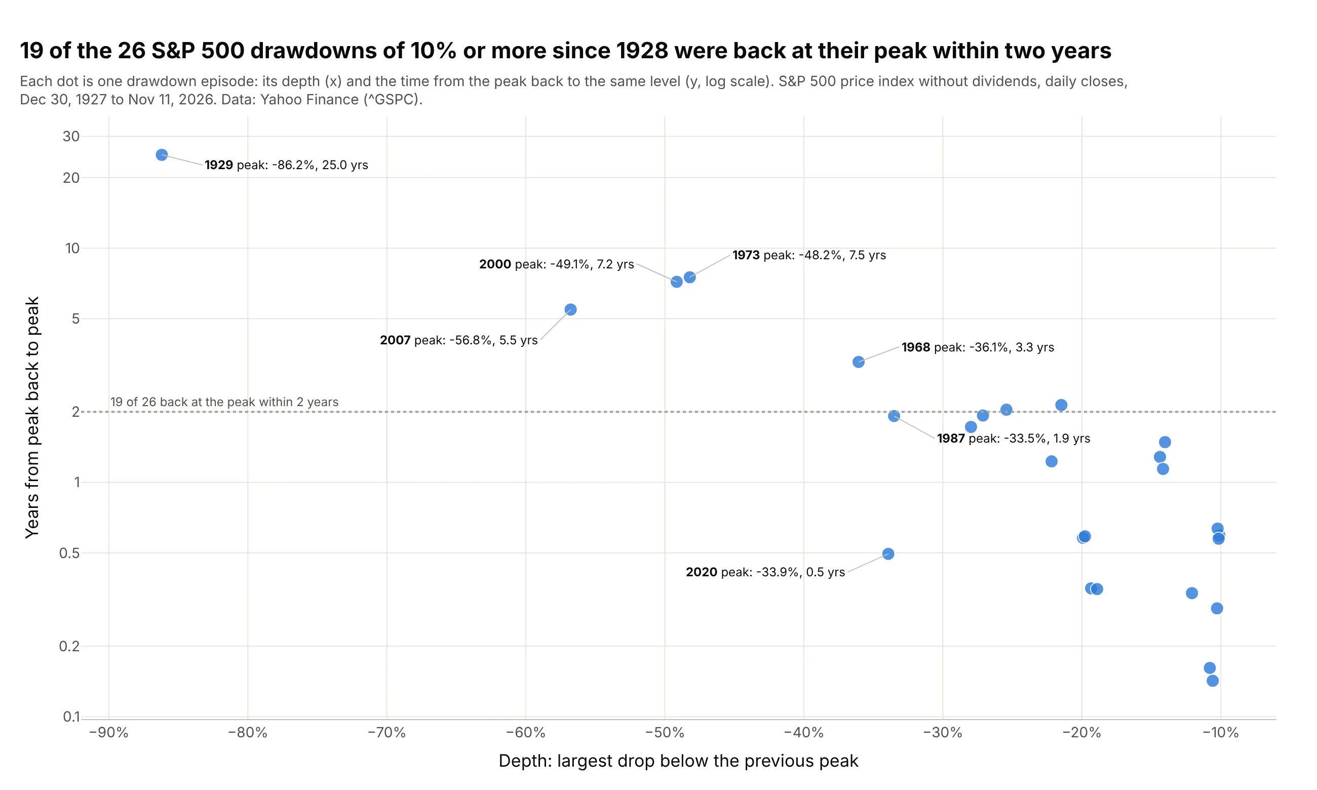
Scatter of 26 S&P 500 drawdown episodes since 1928 with depth on the x axis and years from peak back to peak on a log y axis: 19 dots are below a dotted line at 2 years; labeled outliers are the 1929 peak (-86.2%, 25.0 years), 1973 (-48.2%, 7.5), 2000 (-49.1%, 7.2), 2007 (-56.8%, 5.5), 1968 (-36.1%, 3.3), 1987 (-33.5%, 1.9) and 2020 (-33.9%, 0.5)

Of the 26 times the S&P 500 price index fell 10% or more from a high since 1928, 19 were back at that high within two years. The 1929 episode took 25.0 years in this price-only series. Data: Yahoo Finance, ^GSPC daily close, December 30, 1927 to November 11, 2026.

Tip: to compare episodes rather than dates, turn the drawdown series into a table of episodes and plot depth against recovery time, with a log scale for the time.

Get the data from Yahoo Finance (^GSPC, the S&P 500 price index, daily closes from 1927) and shape it into a table
of drawdown episodes (columns: peak_date, trough_date, recovery_date, depth_pct, days_peak_to_recovery), keeping
episodes of 10% or more.

Build a plotly scatter with depth on x and years from peak to recovery on a log y axis, the peak dates in the hover,
a dotted line at 2 years with the count of episodes below it, and labels on the episodes deeper than 30%.

2. Bitcoin's four drawdowns deeper than 50%

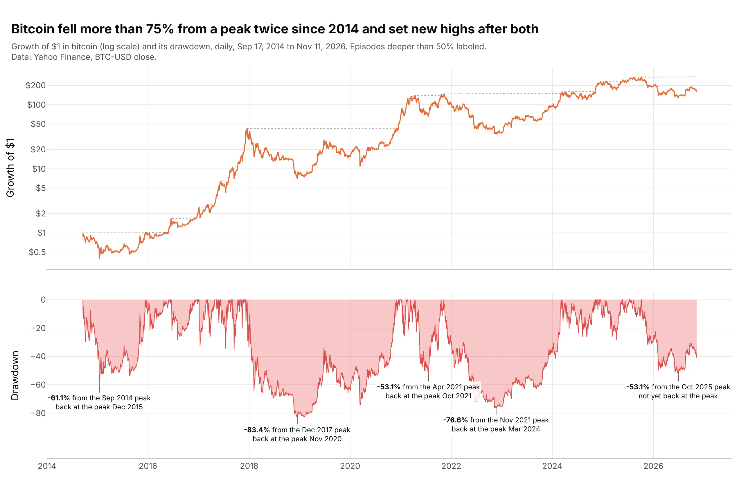
Bitcoin from 2014 to 2026: the growth of $1 on a log scale in orange, and below it the drawdown with labels: 61.1% from the September 2014 peak, back in December 2015; 83.4% from the December 2017 peak, back in November 2020; 53.1% from the April 2021 peak, back in October 2021; 76.6% from the November 2021 peak, back in March 2024; and 53.1% from the October 2025 peak, not yet back

Bitcoin fell 83.4% from its December 2017 peak and 76.6% from its November 2021 peak, and set new highs after both. On November 11, 2026 it was 40.7% below its October 2025 peak. Data: Yahoo Finance, BTC-USD daily close, September 17, 2014 to November 11, 2026.

Tip: for assets that multiplied many times, the log scale on the equity panel is what keeps the early drawdowns visible.

Get the data from Yahoo Finance (BTC-USD daily closes from September 2014) and shape it into a table (columns: date,
close).

Build a plotly drawdown chart with make_subplots: growth of $1 on a log axis with its running peak above, the
drawdown filled to zero below, and every episode deeper than 50% labeled with its depth, its peak month and its
recovery month or "not yet back at the peak".

3. Gold: 8.9 years under water

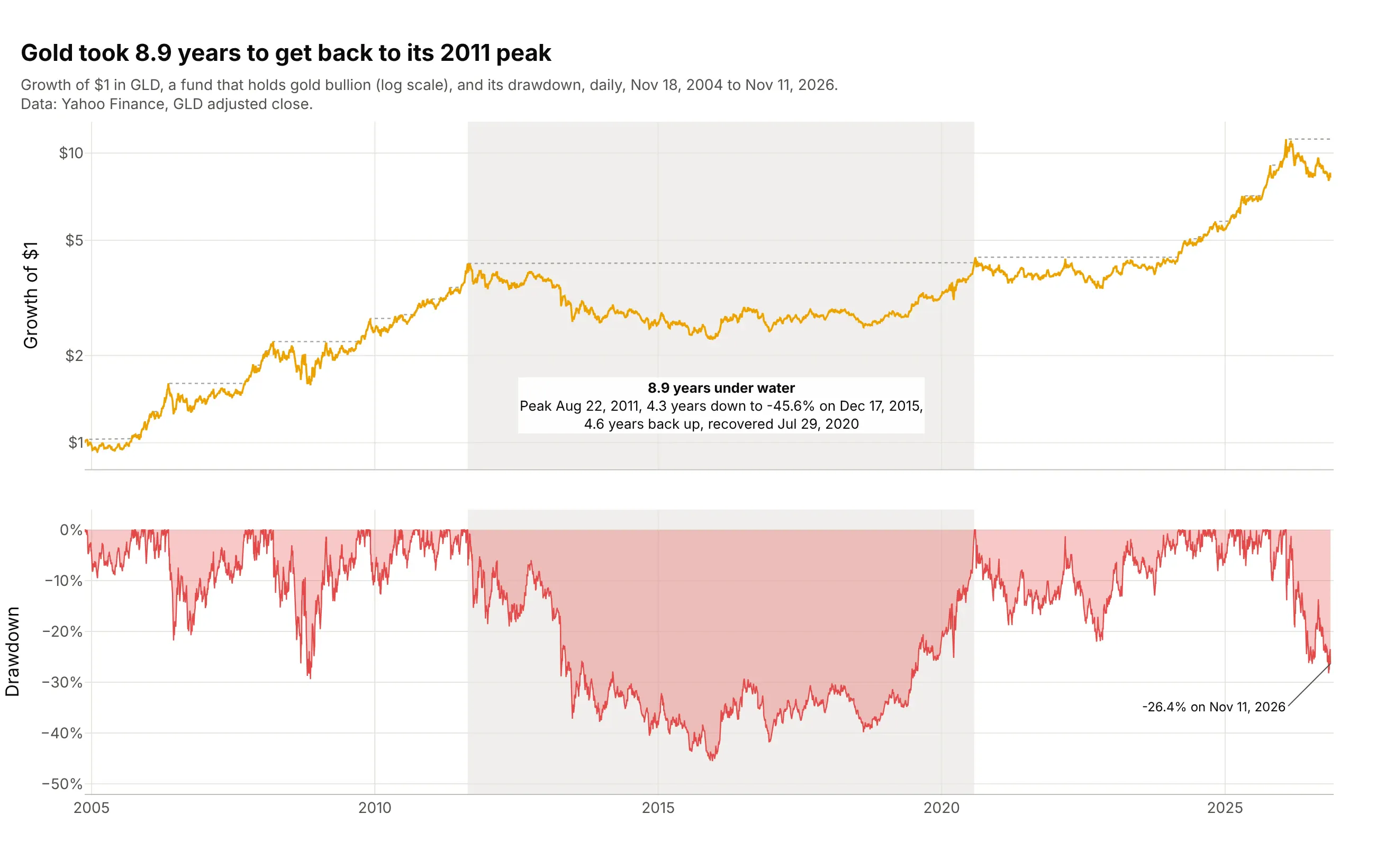
GLD from 2004 to 2026 with the growth of $1 on a log scale and its drawdown below, the period from the August 2011 peak to the July 2020 recovery shaded in both panels and labeled: 8.9 years under water, 4.3 years down to -45.6% on December 17, 2015, 4.6 years back up; a label at the right reads -26.4% on November 11, 2026

Gold's fall after its August 2011 peak was not its deepest possible, 45.6%, but it lasted 8.9 years, 4.3 down and 4.6 back up. Data: Yahoo Finance, GLD (SPDR Gold Shares) adjusted close, November 18, 2004 to November 11, 2026.

Tip: when the story is duration, shade the episode in both panels with add_vrect and put its length in the label.

Get the data from Yahoo Finance (GLD adjusted closes from November 2004) and shape it into a table (columns: date,
adj_close).

Build a plotly drawdown chart with the growth of $1 on a log scale above and the drawdown below on a shared x axis,
shade the longest episode from peak to recovery in both panels, and label it with years down, years back up and the
total time under water.

4. Treasury bond funds by maturity

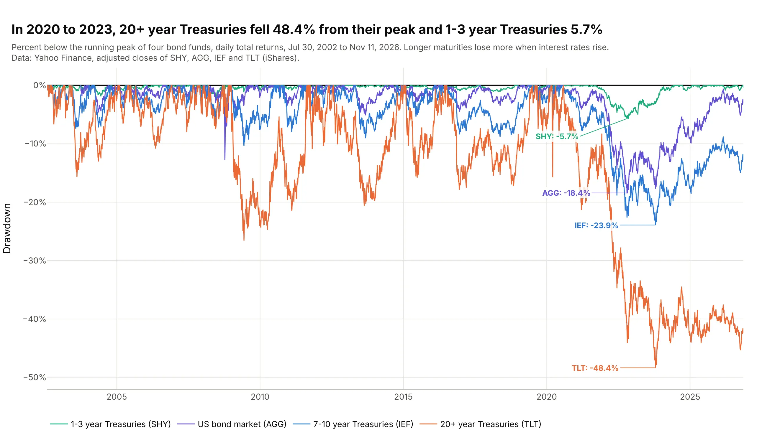
Drawdowns of four bond funds from 2002 to 2026 as lines: 1-3 year Treasuries (SHY) in green never fall more than 5.7%; the US bond market (AGG) in purple reaches 18.4% in 2022; 7-10 year Treasuries (IEF) in blue reach 23.9% and 20+ year Treasuries (TLT) in orange 48.4% in October 2023

When interest rates rose from 2020 to 2023, 20+ year Treasuries fell 48.4% from their August 2020 peak and 1-3 year Treasuries 5.7%, because long bonds lose more value when rates rise. TLT was still 42.4% below its peak on November 11, 2026. Data: Yahoo Finance, adjusted closes of SHY, AGG, IEF and TLT (iShares).

Tip: with four or more series, draw the drawdowns as lines without fill and label each one's deepest point in its own color.

Get the data from Yahoo Finance (adjusted closes of SHY, IEF, TLT and AGG, daily, from July 2002) and shape it into
a table (columns: date, then one column per fund).

Build a plotly chart with one drawdown line per fund on a shared zero line, ordered from short to long maturity,
the deepest point of each labeled in the line's color, and a legend below the plot.

5. Energy stocks: five years down, two years back

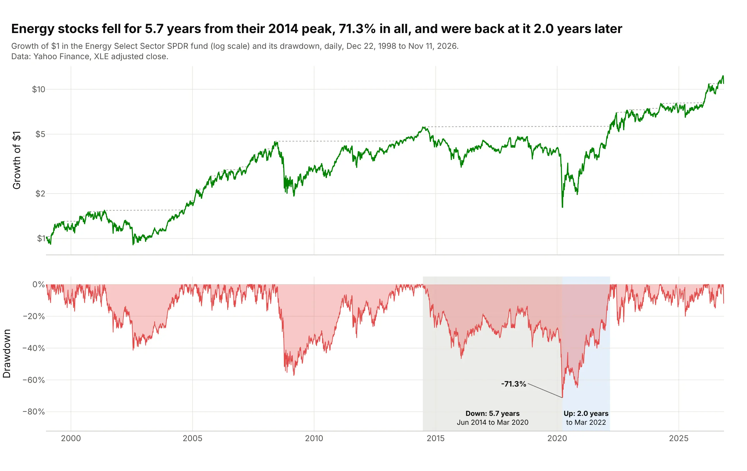
XLE from 1998 to 2026 with the growth of $1 on a log scale and its drawdown below; the 2014 episode is split into a gray band, down 5.7 years from June 2014 to March 2020, and a blue band, up 2.0 years to March 2022, with the trough at -71.3%

The energy sector fell for 5.7 years from its June 2014 peak, 71.3% in all, and was back at that peak 2.0 years after the March 2020 trough. Data: Yahoo Finance, XLE (Energy Select Sector SPDR) adjusted close, December 22, 1998 to November 11, 2026.

Tip: shade peak to trough and trough to recovery in two colors when the two halves of a drawdown have very different lengths.

Get the data from Yahoo Finance (XLE adjusted closes from December 1998) and shape it into a table (columns: date,
adj_close).

Build a plotly drawdown chart with the growth of $1 above and the drawdown below, and split the deepest episode into
two shaded bands, peak to trough in gray and trough to recovery in light blue, each labeled with its length in years.

6. Ten years of health care fund drawdowns

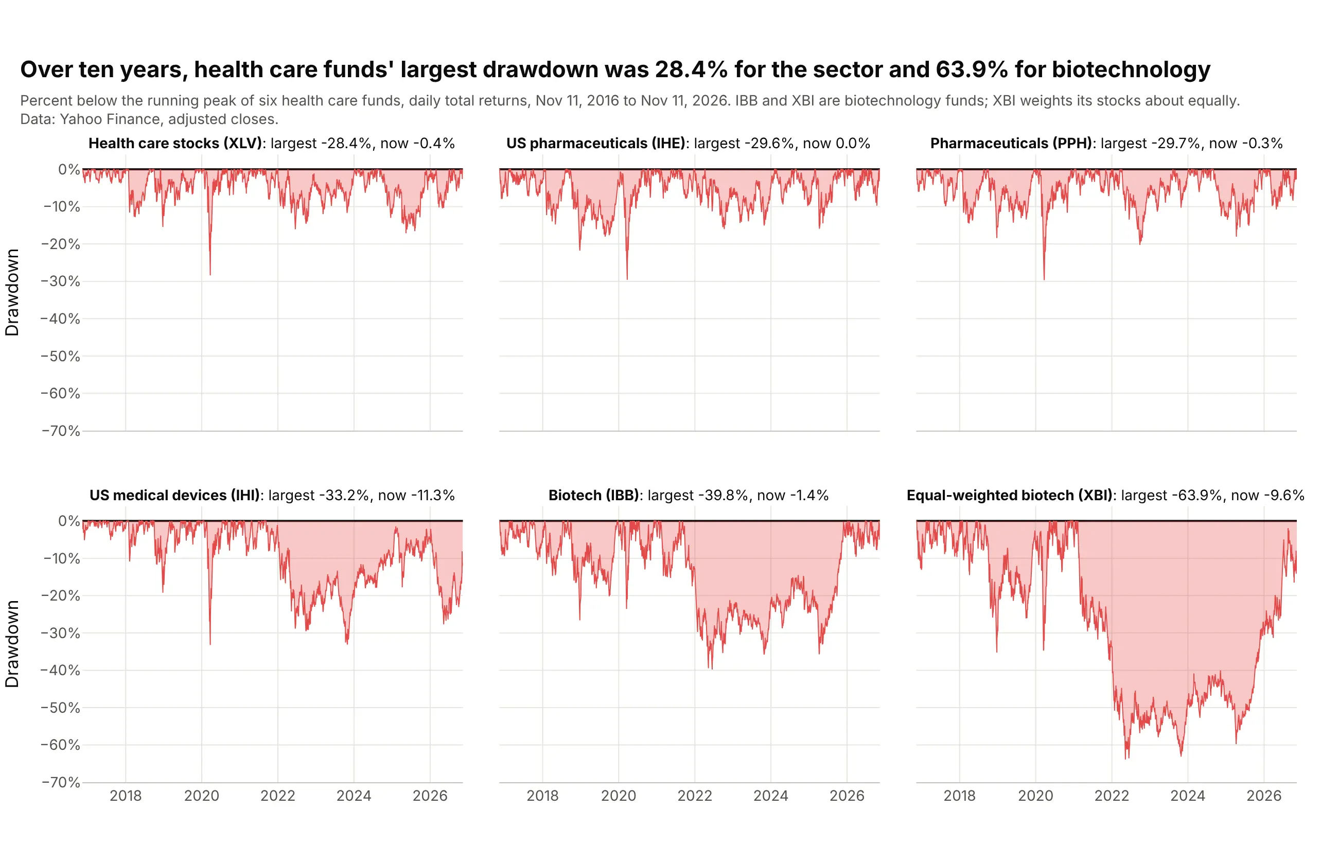
Six small underwater charts on one y range from 0% to -70%, November 2016 to November 2026: health care stocks (XLV) largest -28.4% and now -0.4%, US pharmaceuticals (IHE) -29.6% and 0.0%, pharmaceuticals (PPH) -29.7% and -0.3%, US medical devices (IHI) -33.2% and -11.3%, biotech (IBB) -39.8% and -1.4%, equal-weighted biotech (XBI) -63.9% and -9.6%

Over ten years, the health care sector fund XLV had a largest drawdown of 28.4%, and XBI, a biotechnology fund that weights its stocks about equally, 63.9%, from its February 2021 peak to May 2022. On November 11, 2026, XBI was still 9.6% below that peak, while IBB, a biotechnology fund weighted by company size, had been back at its August 2021 peak since January 2026. Data: Yahoo Finance, adjusted closes of XLV (Health Care Select Sector SPDR), IHE and IHI (iShares), PPH (VanEck), IBB (iShares) and XBI (SPDR), November 11, 2016 to November 11, 2026.

Tip: sort small multiples by maximum drawdown and share the y axis, so depth compares across panels at a glance.

Get the data from Yahoo Finance (adjusted closes of XLV, IHE, PPH, IHI, IBB and XBI, daily, November 2016 to
November 2026) and shape it into a table (columns: date, ticker, adj_close).

Build plotly small multiples (2 rows x 3 columns, shared y axis from 0% to -70%) of each fund's drawdown as a
filled area, sorted by maximum drawdown, with each panel's title giving the fund, its largest drawdown and its
current drawdown.

Another way to see it: the same drawdowns as one scatter of maximum drawdown against return, in example 7, trade the timing for a ranking.

7. Maximum drawdown against annual return

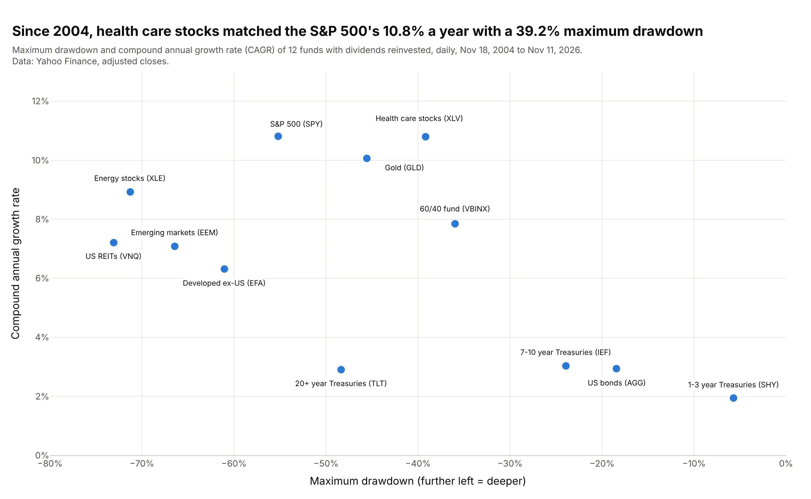
Scatter of 12 funds, November 2004 to November 2026, with maximum drawdown on the x axis and annual growth rate on the y axis: the S&P 500 at -55.2% and 10.8%, health care stocks at -39.2% and 10.8%, gold at -45.6% and 10.1%, energy at -71.3% and 8.9%, 20+ year Treasuries at -48.4% and 2.9%, and 1-3 year Treasuries at -5.7% and 1.9%

Over the same 22 years, health care stocks earned the S&P 500's 10.8% a year with a maximum drawdown of 39.2% instead of 55.2%, and 20+ year Treasuries had a deeper drawdown (48.4%) than gold (45.6%) for under a third of the return. Data: Yahoo Finance, adjusted closes, November 18, 2004 to November 11, 2026.

Tip: compute every asset over the same dates, starting at the youngest one's first day; a maximum drawdown measured over a different period isn't comparable.

Get the data from Yahoo Finance (adjusted closes of SPY, VBINX, AGG, TLT, IEF, SHY, GLD, XLE, XLV, EFA, EEM and VNQ,
daily, from November 18, 2004) and shape it into a table with one row per fund (columns: fund, cagr_pct,
max_drawdown_pct).

Build a plotly scatter with maximum drawdown on x (from -80% to 0%) and compound annual growth rate on y, every fund
labeled by name, and a title that compares the two funds with the same return.

This is the drawdown version of a risk-return chart; the efficient frontier guide draws the same kind of assets with volatility on the x axis.

Drawdown Charts - A Complete Guide

What is a drawdown chart?

A short history

How drawdown is calculated

The running peak, the trough and the recovery

Why a 50% drawdown needs a 100% gain

Daily, monthly or yearly data

Which prices go in

Summary statistics built on drawdowns

Alternatives to a drawdown chart

How to make a drawdown chart

With AI

With Plotly Studio

Make a drawdown chart in Python or JavaScript

Share it

Dos and don'ts

Checklist

Options to customize

More drawdown chart examples

1. Every S&P 500 drawdown of 10% or more since 1928

2. Bitcoin's four drawdowns deeper than 50%

3. Gold: 8.9 years under water

4. Treasury bond funds by maturity

5. Energy stocks: five years down, two years back

6. Ten years of health care fund drawdowns

7. Maximum drawdown against annual return

FAQ

What is a drawdown chart?

Is a drawdown chart the same as an underwater chart?

How is maximum drawdown calculated?

What are peak to trough and recovery time?

How do I plot drawdown in Python?

Why use drawdown instead of volatility?

How many points can a Plotly drawdown chart show?

Can a drawdown chart predict the next drawdown?

What does drawdown mean outside finance?