Chris Parmer

November 9, 2026

Efficient Frontier Charts - A Complete Guide

TL;DR

An efficient frontier chart plots portfolios by risk (the volatility of their returns) on the horizontal axis and expected return on the vertical axis, and draws the curve of portfolios that give the highest expected return for each level of risk. Harry Markowitz introduced the idea in 1952.
Efficient frontiers are also known as the Markowitz frontier, the Markowitz bullet and the portfolio frontier, and are similar to scatter plots of risk against return; when each asset is sized by its market value they become a bubble chart.
The field's conventions: annualized volatility on x and annualized expected return on y, both in percent, a cloud of random portfolios colored by Sharpe ratio, the minimum-variance portfolio, the maximum-Sharpe (tangency) portfolio and a straight capital market line from the risk-free rate through it.
The frontier is only as good as its inputs. Expected returns estimated from the past are noisy, and in our 20 years of data the best mix of 2006-2016 earned a Sharpe ratio of 0.10 over the next ten years. This guide is educational and is not investment advice.
You can make an efficient frontier with Plotly from go.Scatter traces: markers with marker.color for the random portfolios, a line for the frontier, and annotations for the special portfolios. scipy's minimize computes the frontier.

What is an efficient frontier?

Efficient frontiers look like this:

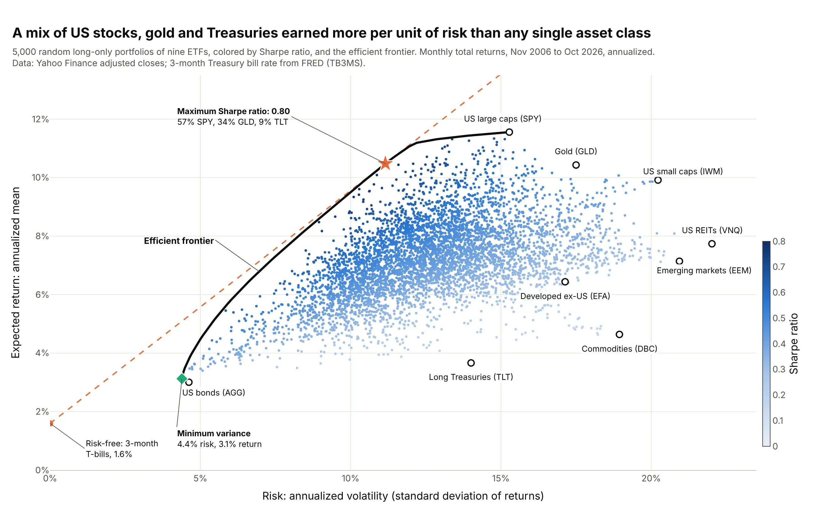
Efficient frontier of nine asset-class ETFs, November 2006 to October 2026: 5,000 random long-only portfolios form a blue cloud colored by Sharpe ratio; a black frontier runs from a green minimum-variance diamond (4.4% risk, 3.1% return) near US bonds up to US large caps (15.3% risk, 11.6% return); an orange star marks the maximum Sharpe portfolio, 0.80 (57% SPY, 34% GLD, 9% TLT), on a dashed capital market line from the 1.6% T-bill rate; the other assets sit inside the frontier

Data: Yahoo Finance monthly adjusted closes of nine exchange-traded funds (ETFs); 3-month Treasury bill rate from FRED (Federal Reserve Economic Data), series TB3MS.

How do you read an efficient frontier? In the example above, notice these things:

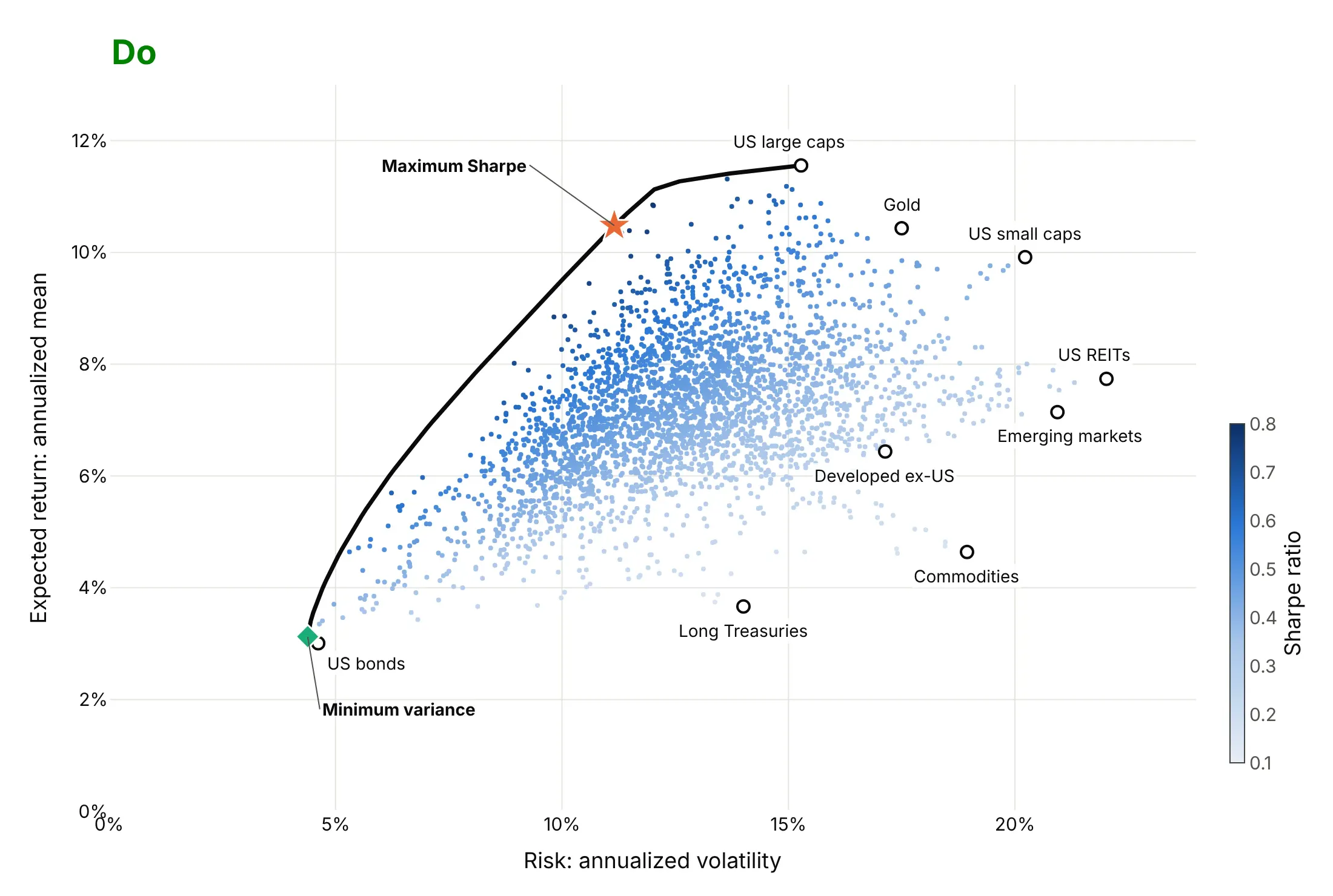
Each open circle is one ETF, a fund that trades like a stock and tracks a broad asset class. Its x position is its risk, the standard deviation of its monthly returns scaled to a year (annualized volatility), and its y position is its average monthly return times 12. US large caps (SPY) returned 11.6% a year with 15.3% volatility from November 2006 to October 2026.
Each small dot is a random portfolio of the nine ETFs with no short sales, and its color is its Sharpe ratio: return above the risk-free rate per unit of risk. The 5,000 dots fill a region, and no mix of these assets can land above or to the left of it.
The black curve is the efficient frontier, the upper-left edge of that region. Every portfolio on it has the highest return available for its risk, so a portfolio below the curve is "inefficient": the same risk could have bought more return.
The green diamond is the minimum-variance portfolio, 93% US bonds (AGG) and 7% commodities (DBC), at 4.4% volatility. That is less than US bonds alone (4.6%), even though commodities alone swung four times as much.
The orange star is the tangency portfolio, 57% US large caps, 34% gold and 9% long Treasuries, with a Sharpe ratio of 0.80 against 0.65 for US large caps alone. The dashed capital market line runs from the 1.6% average Treasury bill rate through it.

It's often used for charts like these:

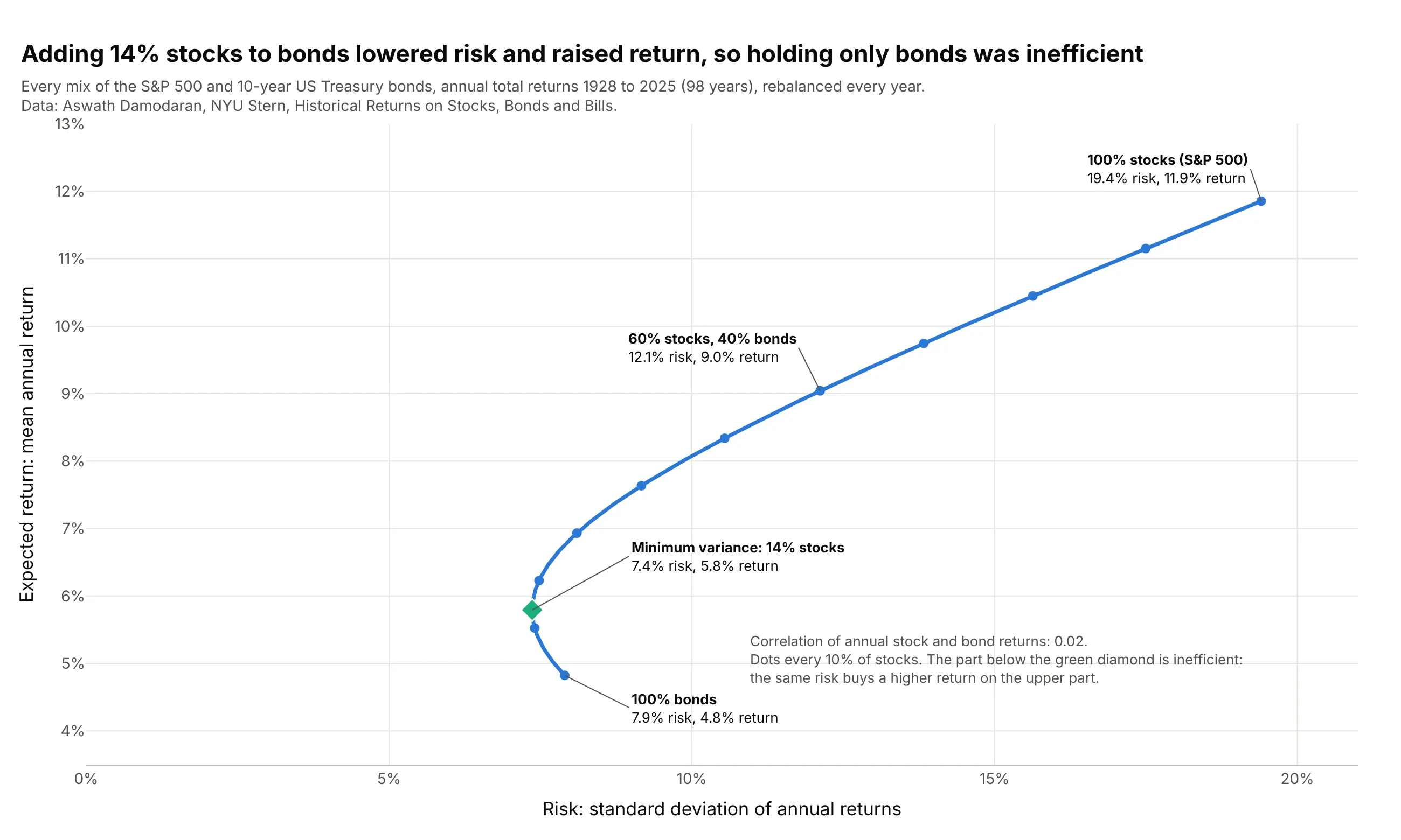
Every mix of the S&P 500 and 10-year US Treasury bonds from 1928 to 2025 as a blue curve with a dot every 10% of stocks: 100% bonds at 7.9% risk and 4.8% return, the curve bending left to a green minimum-variance diamond at 14% stocks with 7.4% risk and 5.8% return, 60% stocks at 12.1% risk and 9.0% return, and 100% stocks at 19.4% risk and 11.9% return; the correlation of annual stock and bond returns was 0.02

Choosing a stock and bond mix. The textbook two-asset frontier shows why a portfolio of only bonds was inefficient from 1928 to 2025: adding 14% stocks lowered the volatility from 7.9% to 7.4% and raised the average return from 4.8% to 5.8%. Data: Aswath Damodaran, NYU Stern, Historical Returns on Stocks, Bonds and Bills.

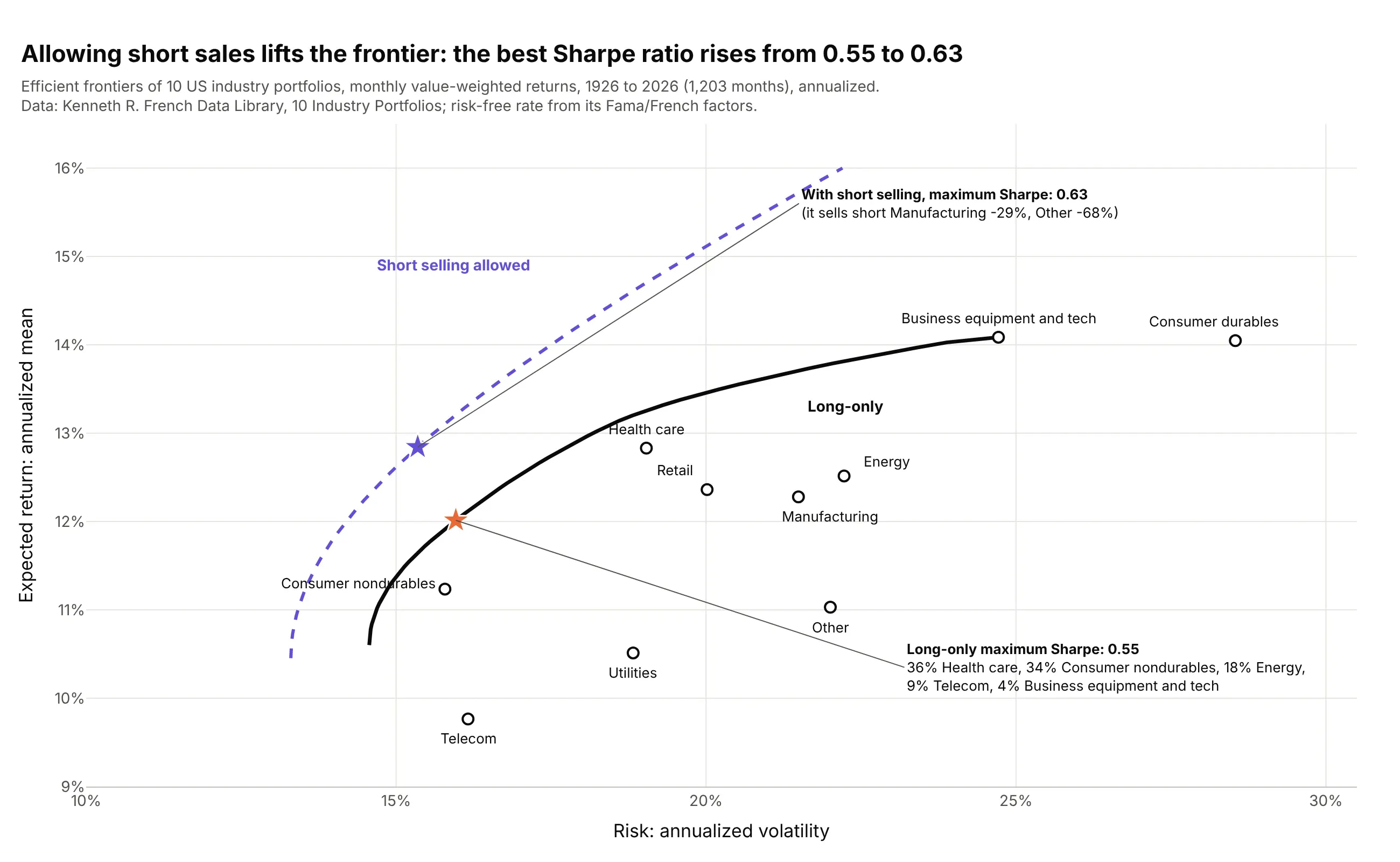
Two efficient frontiers of 10 US industry portfolios from 1926 to 2026: a black long-only curve from about 14.6% to 24.7% risk, with an orange star (maximum Sharpe 0.55: 36% health care, 34% consumer nondurables, 18% energy, 9% telecom, 4% business equipment and tech), and a purple dashed curve with short selling allowed, further up and left, with a purple star at Sharpe 0.63 that sells short manufacturing (-29%) and other (-68%); the 10 industries are labeled open circles

Teaching portfolio theory on industry data. Kenneth French's 10 industry portfolios, 1,203 months from July 1926 to September 2026, are a standard classroom dataset; allowing short sales moves the whole frontier up and lifts the best Sharpe ratio from 0.55 to 0.63. Data: Kenneth R. French Data Library, 10 Industry Portfolios.

A short history

Harry Markowitz published "Portfolio Selection" in The Journal of Finance in March 1952 (Markowitz 1952). His point was that investors care about two things, expected return and risk, measured as variance, and that a portfolio's risk depends on how its assets move together, not only on how risky each one is. In the words of the Nobel committee, this reduced "the multidimensional problem of portfolio choice" to "a conceptually simple two-dimensional problem", known as mean-variance analysis. James Tobin showed in 1958 that adding a risk-free asset makes the best risky portfolio the same for every investor (Tobin 1958), and William Sharpe built that into the capital asset pricing model and the capital market line in 1964 (Sharpe 1964). Markowitz and Sharpe shared the 1990 Nobel Memorial Prize in Economic Sciences with Merton Miller (Nobel Prize press release).

The 1952 paper drew its frontier as a geometric sketch, with no data, so there is no original chart to redraw. Here is his method applied to the returns an investor had in 1952:

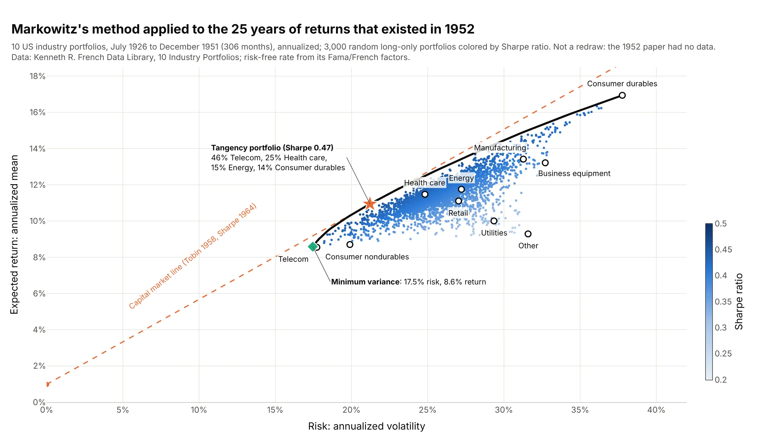
Efficient frontier of 10 US industry portfolios from July 1926 to December 1951, with 3,000 random portfolios colored by Sharpe ratio: the frontier runs from a minimum-variance portfolio at 17.5% risk and 8.6% return near telecom up to consumer durables at 37.8% risk and 16.9% return, with a tangency portfolio at Sharpe 0.47 (46% telecom, 25% health care, 15% energy, 14% consumer durables) and a capital market line labeled Tobin 1958, Sharpe 1964

Data: Kenneth R. French Data Library, 10 Industry Portfolios, July 1926 to December 1951 (306 months). Not a redraw of a figure from the paper.

How the efficient frontier is calculated

The chart rests on a few ideas from statistics that portfolio managers use every day. This section explains them in plain terms, using the stock and bond data from the second example.

Return, risk and the Sharpe ratio

The expected return of an asset is estimated as the average of its past returns, here scaled to a year: the S&P 500 returned 11.9% a year on average from 1928 to 2025. Risk is the standard deviation of those returns, the typical distance between one year's return and the average, which investors call volatility: 19.4% for the S&P 500 and 7.9% for 10-year Treasury bonds. A portfolio's expected return is the weighted average of its assets' returns, so a 60/40 mix of stocks and bonds averaged 0.6 × 11.9% + 0.4 × 4.8% = 9.0%.

The Sharpe ratio, from Sharpe (1966), divides a portfolio's return above the risk-free rate (the yield on short-term Treasury bills) by its volatility, so it measures return per unit of risk. With a 1.6% Treasury bill rate, US large caps scored (11.6 - 1.6) / 15.3 = 0.65 in the main example.

Why diversification bends the curve

A portfolio's volatility is not the weighted average of its assets' volatilities, because the ups of one asset partly cancel the downs of another. How much they cancel depends on their correlation, a number from -1 (they always move in opposite directions) to +1 (they always move together). With weights w and 1 - w, the variance of a two-asset portfolio is w²σ₁² + (1 - w)²σ₂² + 2w(1 - w)ρσ₁σ₂, where σ is each asset's volatility and ρ (rho) their correlation. Only at ρ = +1 is the mix's volatility the straight weighted average; any lower correlation pulls it to the left:

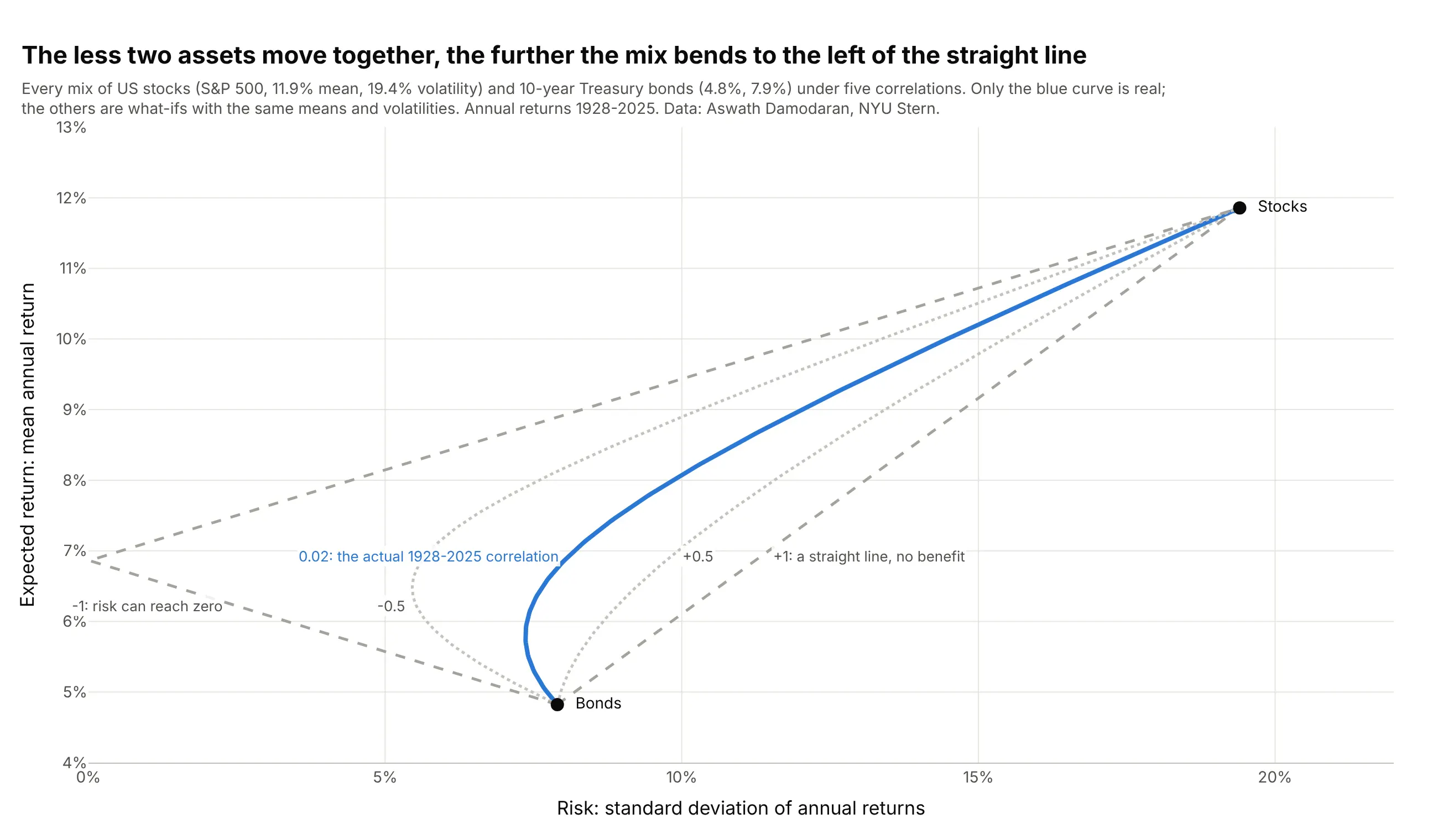
Five curves of every mix of US stocks (11.9% mean, 19.4% volatility) and 10-year Treasury bonds (4.8%, 7.9%) under correlations of +1, +0.5, 0.02, -0.5 and -1: at +1 a straight dashed line joins the two assets, at -0.5 and -1 the curves bend far to the left and at -1 they touch zero risk; the real correlation of 0.02 is the solid blue curve, bending left to about 7.4% risk

Data: Aswath Damodaran, NYU Stern, annual returns 1928-2025. Only the blue curve uses the actual correlation; the other four are what-ifs with the same means and volatilities.

Stocks and bonds had a correlation of 0.02 over those 98 years, almost no relation, so the curve bends left of both ends. That bend is diversification, and with more than two assets the frontier is the left edge of all the bends at once.

Mean-variance optimization

Finding the frontier is an optimization problem: for each target return, find the weights that minimize the portfolio's variance, subject to the weights adding up to 100% (and, usually, to no weight being negative, meaning no short selling). Markowitz showed in 1956 how to solve it, and today it is a quadratic program that scipy's minimize or a dedicated solver handles in milliseconds. Repeating it for 60 target returns gives 60 points on the curve. The minimum-variance portfolio is the leftmost point, and the tangency portfolio is the one with the highest Sharpe ratio, where a straight line from the risk-free rate just touches the curve.

That straight line is the capital market line. Mixing the tangency portfolio with Treasury bills moves you along it: 50% in each halves both the risk and the excess return. Because the line lies above the curve everywhere except at the tangency point, the theory says every investor should hold the same risky mix and set their risk with the share in bills.

The limits

The math is exact, but the inputs are estimates, and Markowitz's model inherits every error in them:

Expected returns are hard to estimate. Twenty years of monthly returns pin down an asset's volatility well and its average return badly, and the optimizer puts the most weight on the assets whose returns happen to be overestimated. That is the problem behind the title of Michaud (1989), "The Markowitz Optimization Enigma: Is 'Optimized' Optimal?". Example 5 below redraws the frontier from 200 resampled histories, and example 6 shows what happened when the best portfolio of 2006-2016 was held for the next decade.
The past is not the future. Correlations and returns change: the least risky industry mix had 6.8% volatility in the 1950s and 23.2% in the 1930s (example 7).
Volatility is not the only risk. Variance treats gains and losses alike and misses rare crashes, liquidity and inflation, and the model ignores fees and taxes.
Naive mixes are hard to beat. In this guide's data, equal weights in all nine ETFs earned a Sharpe ratio of 0.57 in 2016-2026, against 0.10 for the previous decade's optimal mix. DeMiguel, Garlappi and Uppal (2009) study this comparison of optimal and naive (1/N) diversification across many models and datasets.

Alternatives to an efficient frontier

Here's the same set of nine asset-class ETFs drawn six ways. Some are better for the question, some worse, some just different:

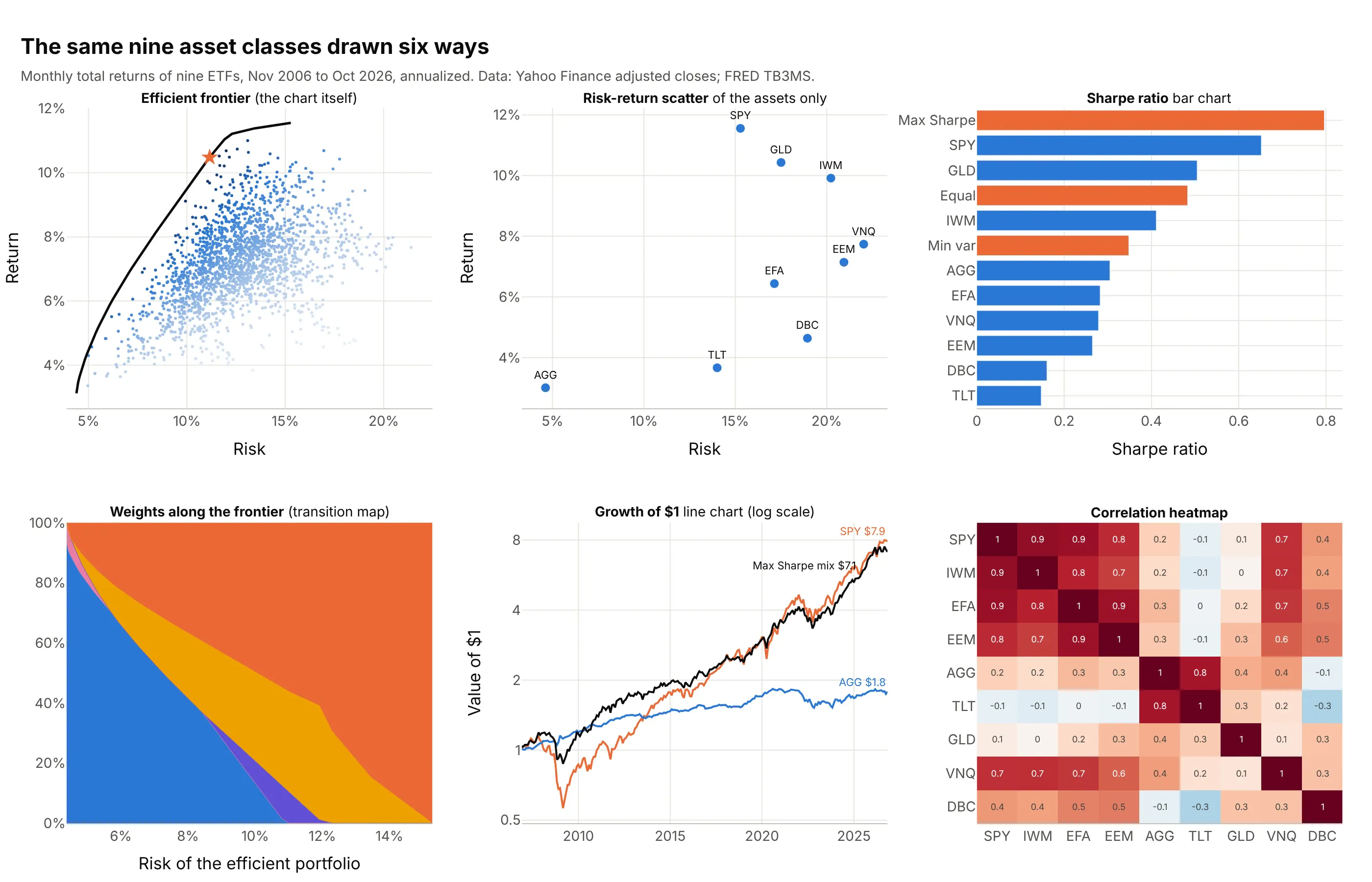
Six small charts of the same nine ETFs from 2006 to 2026: the efficient frontier with random portfolios; a risk-return scatter of the nine assets only; a horizontal bar chart of Sharpe ratios with the maximum Sharpe mix (0.80) at the top, then SPY, GLD and the equal-weight mix; a stacked area of the weights along the frontier; a log-scale line chart of the growth of $1, SPY to $7.9, the maximum Sharpe mix to $7.1 and AGG to $1.8; and a correlation heatmap

Efficient frontier (the chart itself). It shows every possible mix, the best ones and how far each asset is from them on one chart, which is why portfolio managers and textbooks use it. It hides what the portfolios hold.
Risk-return scatter plot of the assets (works too, for a first look). Plotting only the assets compares them fairly and is easy to read, but it can't show that a mix beats them all. Sizing the points by market value turns it into a bubble chart (example 3 below).
Bar chart of Sharpe ratios (better for ranking). Sorted bars rank return per unit of risk precisely, including portfolios, but drop the two separate dimensions.
Weights along the frontier (different). A stacked area chart of weights against risk, a transition map, answers "what is in the efficient portfolios?", which the frontier can't (example 4 below).
Growth of $1 line chart (different). It shows the path, including the 2008 drawdown, that a single volatility number summarizes. It is the chart people trust most and the hardest to compare many portfolios on.
Correlation heatmap (different, and a good companion). It shows the input that makes diversification work, such as US large caps' correlation of 0.09 with gold and -0.08 with long Treasuries, but not the result.

How to make an efficient frontier

With AI

ChatGPT, Claude Code, GitHub Copilot, Cursor, and other AI tools are excellent at writing Plotly code. Name Plotly in the prompt, and say which constraints the portfolios have and how to annualize:

Make a plotly efficient frontier chart from prices.csv (columns: month, then one column of monthly adjusted
closes per asset).

- Compute monthly returns; annualize the mean (x12) and the covariance (x12). Risk-free rate 1.6% a year.
- Draw 5,000 random long-only portfolios as go.Scatter markers colored by Sharpe ratio with a colorbar.
- Compute the long-only efficient frontier with scipy.optimize.minimize (60 target returns) and draw it as a line.
- Mark the minimum-variance portfolio and the maximum Sharpe portfolio, print the latter's weights in an
  annotation, and draw the capital market line from the risk-free rate through it.
- Risk (annualized volatility) on x and expected return on y, both in %; label each asset on the chart.
- Check: print each asset's annualized mean, volatility and Sharpe ratio, and the two portfolios' weights.

With Plotly Studio

Plotly Studio is a desktop app where you point an AI at a dataset and it builds charts and a Dash app around your questions. Ask for an efficient frontier the same way:

Show the efficient frontier of these assets with random portfolios colored by Sharpe ratio, a date range picker for the period used to estimate returns, a switch to allow short selling, and a table of the maximum Sharpe portfolio's weights.

Make an efficient frontier in Python or JavaScript

This is the code AI tools write under the hood. Plotly draws the chart, and scipy finds the frontier: for each target return, minimize looks for the weights with the lowest volatility. prices.csv holds one column of monthly prices per asset, like the nine ETFs above:

import numpy as np
import pandas as pd
import plotly.graph_objects as go
from scipy.optimize import minimize

prices = pd.read_csv("prices.csv", index_col="month")  # monthly adjusted closes, one column per asset
r = prices.pct_change().dropna()
mu = r.mean().values * 12   # expected return per year
cov = r.cov().values * 12   # covariance per year
rf = 0.016                  # risk-free rate: average 3-month T-bill yield
n = len(mu)
vol = lambda w: np.sqrt(w @ cov @ w)
budget = {"type": "eq", "fun": lambda w: w.sum() - 1}  # weights add up to 100%
long_only = [(0, 1)] * n                                # no short selling

def min_risk(target):  # the least risky portfolio with this expected return
    hit = {"type": "eq", "fun": lambda w: w @ mu - target}
    return minimize(vol, np.full(n, 1 / n), bounds=long_only, constraints=[budget, hit]).x

targets = np.linspace(mu.min(), mu.max(), 60)
frontier = [vol(min_risk(t)) for t in targets]
w_t = minimize(lambda w: -(w @ mu - rf) / vol(w), np.full(n, 1 / n), bounds=long_only, constraints=[budget]).x
W = np.random.default_rng(0).dirichlet(np.ones(n), 5000)  # random long-only portfolios
cloud_vol, cloud_ret = np.sqrt(np.einsum("ij,jk,ik->i", W, cov, W)), W @ mu

fig = go.Figure()
fig.add_scatter(x=cloud_vol, y=cloud_ret, mode="markers", name="Random portfolios",
                marker=dict(size=4, color=(cloud_ret - rf) / cloud_vol, colorscale="Blues",
                            showscale=True, colorbar_title="Sharpe"))
fig.add_scatter(x=frontier, y=targets, mode="lines", name="Efficient frontier", line=dict(color="black", width=3))
fig.add_scatter(x=np.sqrt(np.diag(cov)), y=mu, mode="markers+text", text=prices.columns,
                textposition="top center", name="Assets", marker=dict(color="white", line_width=2))
fig.add_scatter(x=[0, vol(w_t) * 2], y=[rf, rf + 2 * (w_t @ mu - rf)], mode="lines", name="Capital market line",
                line=dict(dash="dash", color="orange"))
fig.update_layout(xaxis=dict(title="Risk (annualized volatility)", tickformat=".0%", rangemode="tozero"),
                  yaxis=dict(title="Expected return (annualized)", tickformat=".0%"),
                  legend=dict(orientation="h", y=-0.2))
fig.show()

On the nine ETFs above it finds the same maximum Sharpe mix as the main example: 57% SPY, 34% GLD and 9% TLT. To allow short selling, change the bounds to (-1, 1). For more than a few dozen assets, a quadratic programming library such as cvxpy or PyPortfolioOpt is faster and more reliable than minimize.

In JavaScript, plotly.js draws the two-asset curve from the stock and bond example directly, since every mix of two assets lies on it:

<div id="chart"></div>
<script src="https://cdn.plot.ly/plotly-4.1.1.min.js"></script>
<script>
  // US stocks (S&P 500) and 10-year Treasury bonds, annual returns 1928-2025 (Damodaran, NYU Stern)
  const stocks = {mean: 11.85, sd: 19.40}, bonds = {mean: 4.82, sd: 7.90}, rho = 0.02;
  const x = [], y = [], text = [];
  for (let i = 0; i <= 100; i++) {
    const w = i / 100;  // share in stocks
    x.push(Math.sqrt((w * stocks.sd) ** 2 + ((1 - w) * bonds.sd) ** 2 + 2 * w * (1 - w) * rho * stocks.sd * bonds.sd));
    y.push(w * stocks.mean + (1 - w) * bonds.mean);
    text.push(i + "% stocks");
  }
  Plotly.newPlot("chart", [
    {x: x, y: y, text: text, mode: "lines", line: {color: "#2a78d6", width: 3}, hovertemplate: "%{text}<extra></extra>"},
    {x: [bonds.sd, stocks.sd], y: [bonds.mean, stocks.mean], text: ["Bonds", "Stocks"], mode: "markers+text",
     textposition: "middle right", marker: {size: 10, color: "black"}}
  ], {
    width: 900, height: 500, showlegend: false,
    xaxis: {title: {text: "Risk: standard deviation of annual returns"}, ticksuffix: "%", rangemode: "tozero"},
    yaxis: {title: {text: "Expected return: mean annual return"}, ticksuffix: "%"}
  });
</script>

Share it

Every Plotly chart has a Share chart button (the cloud icon in its toolbar) that uploads it to Plotly Cloud and gives you a link. Only you can see it until you change its visibility.

For a live app, put the chart in a Dash app and publish it with the Plotly Cloud CLI. Coding agents can run these commands for you:

pip install "dash[cloud]"
plotly user login
plotly app publish

If your data has to stay in your own cloud or data center, publish to Dash Enterprise instead.

Dos and don'ts

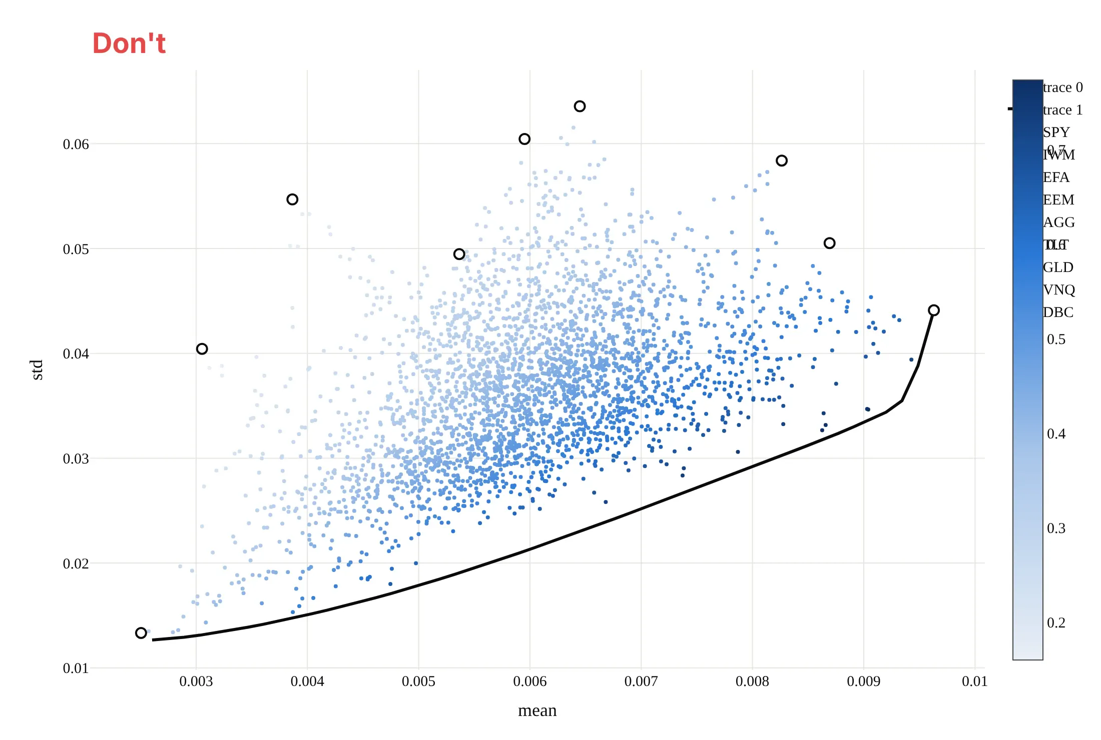
Most mistakes in published frontiers come from the units: returns left as monthly decimals, or risk and return on the wrong axes. Here is the main example both ways, in the same colors.

Don't plot monthly means and standard deviations as raw decimals, put return on x and risk on y against the field's convention, leave the column names "mean" and "std" as axis titles, identify the assets only through a legend of tickers that collides with the colorbar, or keep a serif default font:

The same nine ETFs and random portfolios with mean monthly return (0.003 to 0.01) on the x axis and monthly standard deviation (0.01 to 0.06) on the y axis, so the frontier runs along the bottom right; the axis titles read mean and std, the assets are unlabeled circles, a legend listing trace 0, trace 1 and nine tickers overlaps the colorbar, and the font is serif

Do put annualized volatility on x and annualized expected return on y in percent, label each asset on the chart, and mark the frontier, the minimum-variance portfolio and the maximum Sharpe portfolio:

The same chart with risk as annualized volatility on x from 0% to 23% and expected return as annualized mean on y from 0% to 13%, the nine assets labeled by name, the black frontier, a green minimum-variance diamond and an orange maximum Sharpe star, in Inter

Checklist

Annualize both axes the same way (mean × 12 and standard deviation × √12 for monthly data) and say so.
State the period, the data source and the risk-free rate, because the frontier changes with all three.
Say whether short selling is allowed; long-only and unconstrained frontiers differ a lot.
Use total returns (with dividends reinvested), not price returns.
Show the inputs next to the result, for example the correlation heatmap or the weights along the frontier.

Don't

Present a frontier estimated from the past as a forecast, or its tangency portfolio as a recommendation.
Mix daily, monthly and annual statistics on one chart.
Draw the capital market line from a risk-free rate taken from a different period than the returns.
Hide the inefficient lower half without saying it exists; when you do draw it, make it dashed or lighter.

Options to customize

An efficient frontier in Plotly is built from go.Scatter traces and annotations, so these are the options that matter most. The full lists are in the scatter trace reference, the colorscales documentation and the text and annotations documentation.

marker.color with colorscale, cmin and cmax: color the random portfolios by Sharpe ratio on a sequential scale.
marker.colorbar (title, len, y): a short colorbar that leaves room for labels.
go.Scattergl: WebGL instead of SVG when you draw more than about 10,000 random portfolios.
mode="lines" with line.dash: the frontier solid, its inefficient half and the capital market line dashed.
marker.symbol ("star", "diamond", "circle-open"): the tangency portfolio, the minimum-variance portfolio and the single assets.
fig.add_annotation(ax=..., ay=..., axref="x", ayref="y"): labels with arrows placed at data coordinates, for the special portfolios and their weights.
hovertemplate with customdata: show each portfolio's weights on hover.
xaxis.ticksuffix="%" or tickformat=".0%": percent on both axes, and rangemode="tozero" so the capital market line starts at zero risk.
marker.size with sizemode="area" and sizeref: size assets by market value for a bubble version.
stackgroup: the weights along the frontier as a stacked area (transition map).

More efficient frontier examples

Seven more efficient frontier charts built from real public data, each with its source, the technique that makes it work, and a prompt to rebuild it. They cover sectors, single stocks, the weights behind the curve, and three ways to see how uncertain a frontier is.

1. Energy is the most volatile sector, and the best sector mix still holds some

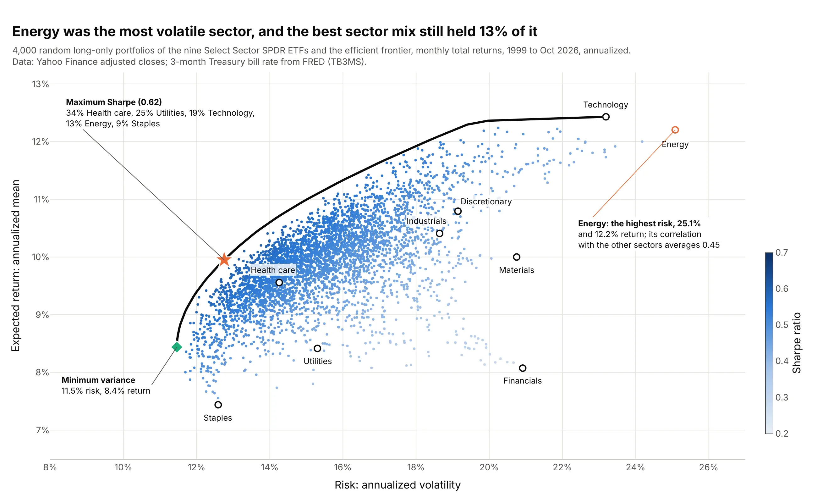
Efficient frontier of the nine Select Sector SPDR ETFs from January 1999 to October 2026 with 4,000 random portfolios colored by Sharpe ratio: energy, highlighted in orange, has the highest risk at 25.1% and 12.2% return, with an average correlation of 0.45 with the other sectors; the maximum Sharpe portfolio (0.62) holds 34% health care, 25% utilities, 19% technology, 13% energy and 9% staples; the minimum-variance portfolio sits at 11.5% risk and 8.4% return

Energy had the highest volatility of the nine sectors, 25.1%, yet the maximum Sharpe sector mix held 13% of it, because its average correlation with the other sectors, 0.45, was the second lowest after utilities. Data: Yahoo Finance monthly adjusted closes of the Select Sector SPDR ETFs, January 1999 to October 2026; FRED TB3MS.

Tip: give the asset you want to talk about its own outline color and leave the others in ink.

Get the data from Yahoo Finance (monthly adjusted closes of the nine original Select Sector SPDR ETFs: XLB, XLE,
XLF, XLI, XLK, XLP, XLU, XLV, XLY, from December 1998) and FRED series TB3MS (3-month Treasury bill rate), and shape
it into a table (columns: month, then one column of monthly returns per ETF).

Build a plotly efficient frontier: 4,000 random long-only portfolios colored by Sharpe ratio, the long-only frontier
as a black line, the sectors as labeled open circles with energy outlined in orange, and annotations for the
maximum Sharpe weights and the minimum-variance portfolio.

2. Ten drugmakers together are steadier than the steadiest one

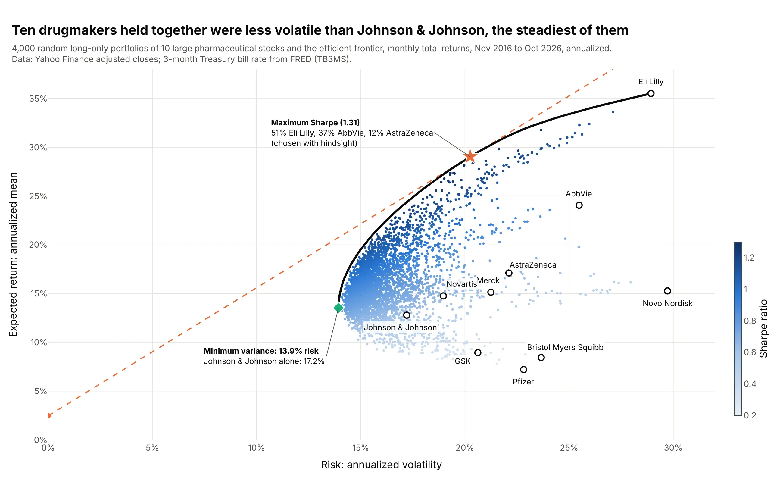
Efficient frontier of 10 large pharmaceutical stocks from November 2016 to October 2026 with a capital market line: Eli Lilly at the top right with 35.5% return and 28.9% risk, AbbVie at 24.1% and 25.5%, Johnson & Johnson at 12.8% and 17.2%, Pfizer lowest at 7.2%; the minimum-variance portfolio is at 13.9% risk, left of every single stock, and the maximum Sharpe portfolio (1.31, chosen with hindsight) holds 51% Eli Lilly, 37% AbbVie and 12% AstraZeneca

The least risky mix of 10 drugmakers had 13.9% volatility, below Johnson & Johnson's 17.2%, the lowest of any single stock. The maximum Sharpe mix, 51% Eli Lilly, is pure hindsight: it picks the decade's winners. Data: Yahoo Finance monthly adjusted closes (LLY, JNJ, MRK, PFE, ABBV, BMY, AZN, NVS, GSK, NVO), November 2016 to October 2026; FRED TB3MS.

Tip: write "chosen with hindsight" next to a tangency portfolio built from past returns of single stocks.

Get the data from Yahoo Finance (monthly adjusted closes of LLY, JNJ, MRK, PFE, ABBV, BMY, AZN, NVS, GSK and NVO)
and FRED series TB3MS, and shape it into a table (columns: month, then one column of monthly returns per stock)
for November 2016 to October 2026.

Build a plotly efficient frontier with random long-only portfolios colored by Sharpe ratio, company names as labels,
the minimum-variance portfolio compared in an annotation with the least volatile stock, and the capital market line.

3. Risk and return of 49 industries, sized by market value

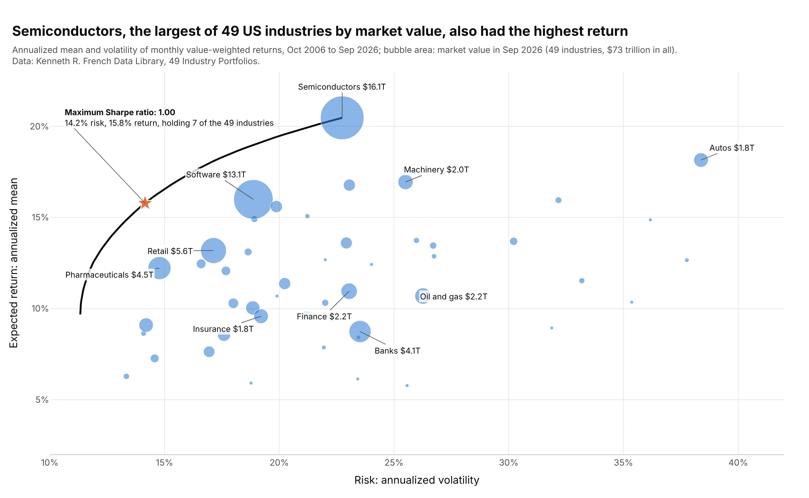
Bubble chart of 49 US industry portfolios, October 2006 to September 2026, risk on x and return on y, sized by market value: semiconductors are the largest ($16.1 trillion) with the highest return, about 20.5% at 22.7% risk, then software ($13.1 trillion), retail, pharmaceuticals and banks; the black efficient frontier ends at semiconductors, and the maximum Sharpe portfolio (1.00) sits at 14.2% risk and 15.8% return, holding 7 of the 49 industries

Semiconductors were the largest of 49 US industries by market value, $16.1 trillion of $73 trillion, and had the highest average return, 20.5% a year. The maximum Sharpe portfolio held only 7 of the 49 industries. Data: Kenneth R. French Data Library, 49 Industry Portfolios (value-weighted returns, number of firms and average firm size).

Tip: with dozens of assets, drop the random cloud and let bubble size carry the second message; sizemode="area" keeps the sizes honest.

Get the data from the Kenneth R. French Data Library (49_Industry_Portfolios_CSV.zip: value-weighted monthly
returns, number of firms and average firm size) and shape it into a table with one row per industry (columns:
industry, mean_return, volatility, market_value) for the last 240 months, plus the covariance matrix.

Build a plotly scatter with marker.size = market_value (sizemode="area"), the ten largest industries labeled, and
the long-only efficient frontier and its maximum Sharpe portfolio on top.

4. What the efficient portfolios hold

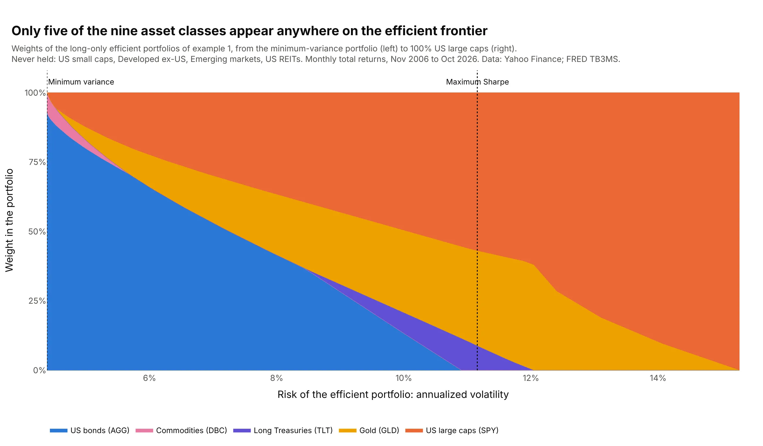
Stacked area chart of the weights of the long-only efficient portfolios from the main example, from the minimum-variance portfolio at 4.4% risk on the left to 100% US large caps at 15.3% on the right: US bonds fall from 93% to zero by about 11% risk, gold rises to about 40% around 12% risk and then falls, long Treasuries appear as a thin band between about 8% and 12%, commodities only at the far left, and US large caps grow to 100%; a dotted line marks the maximum Sharpe portfolio at 11.2% risk

Only five of the nine asset classes appear anywhere on the frontier, and small caps, developed and emerging markets outside the US, and real estate investment trusts (REITs) are never held. A frontier alone can't show this. Data: Yahoo Finance monthly adjusted closes, November 2006 to October 2026; FRED TB3MS.

Tip: use stackgroup with risk on x, so each vertical slice of the chart is one portfolio on the frontier.

Get the data from Yahoo Finance (monthly adjusted closes of SPY, IWM, EFA, EEM, AGG, TLT, GLD, VNQ and DBC) and
FRED series TB3MS, and shape it into a table of the weights of 80 long-only efficient portfolios (columns: volatility,
then one weight column per ETF).

Build a plotly stacked area chart (go.Scatter with stackgroup) of the weights against volatility, one color per
asset class, leaving out assets that never get weight, and dotted vertical lines at the minimum-variance and
maximum Sharpe portfolios.

5. The same data supports a wide band of frontiers

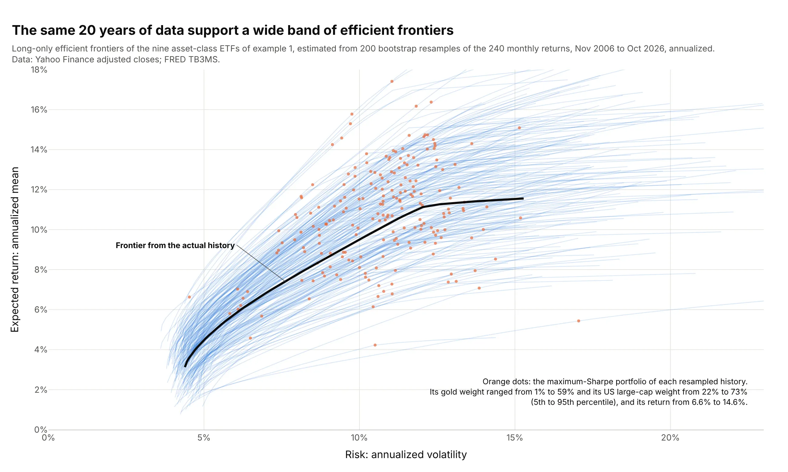
200 thin blue efficient frontiers estimated from bootstrap resamples of the 240 monthly returns of the nine ETFs, spread from about 6% to over 16% return at the high end, with the frontier from the actual history in black through the middle and 200 orange dots for each resample's maximum Sharpe portfolio scattered between about 4% and 17% return; a note says the tangency portfolio's gold weight ranged from 1% to 59% and its US large-cap weight from 22% to 73% (5th to 95th percentile)

Redrawing the 240 months with replacement 200 times gives 200 plausible histories, and their maximum Sharpe portfolios held anywhere from 1% to 59% gold (5th to 95th percentile). This spread is estimation error, and averaging the resampled portfolios is the idea behind resampled efficiency. Data: Yahoo Finance monthly adjusted closes, November 2006 to October 2026; FRED TB3MS.

Tip: draw all resampled frontiers as one trace with None between them and an alpha of about 0.2, so 200 lines render as fast as one.

Get the data from Yahoo Finance (monthly adjusted closes of SPY, IWM, EFA, EEM, AGG, TLT, GLD, VNQ and DBC) and
FRED series TB3MS, and shape it into a table of monthly returns (columns: month, one column per ETF) for
November 2006 to October 2026.

Draw 200 bootstrap samples of the months with numpy (fixed seed), compute each sample's long-only frontier and
maximum Sharpe portfolio, and build a plotly chart with the 200 frontiers as one translucent line trace, the
tangency portfolios as orange dots, and the full-sample frontier in black.

6. The best portfolio of 2006-2016, held for the next decade

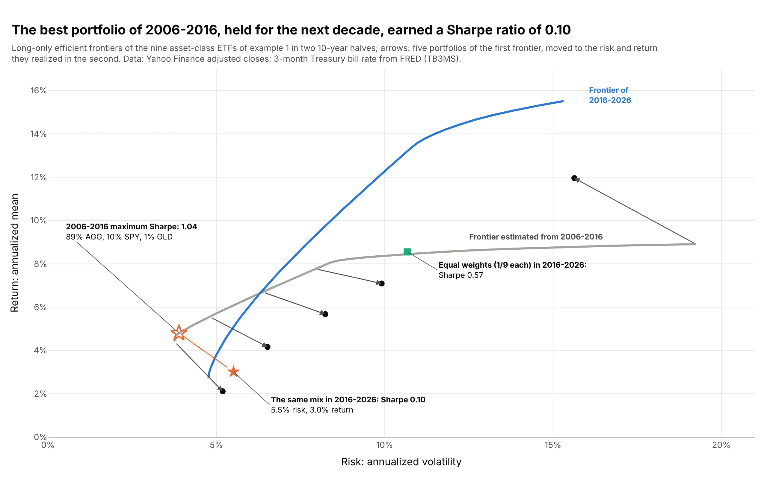
Two efficient frontiers of the nine ETFs: a gray one estimated from 2006-2016 that is flat at about 8% to 9% return, and a blue one for 2016-2026 that rises to 15.5%; arrows move five portfolios of the gray frontier to where they landed in 2016-2026; the 2006-2016 maximum Sharpe portfolio (Sharpe 1.04: 89% AGG, 10% SPY, 1% GLD) moves to 5.5% risk and 3.0% return, a Sharpe ratio of 0.10, while equal weights earned a Sharpe ratio of 0.57

The maximum Sharpe mix of November 2006 to October 2016, 89% bonds, had a Sharpe ratio of 1.04 in that decade and 0.10 in the next, when bonds returned 1.6% a year. Equal weights in all nine earned 0.57. Data: Yahoo Finance monthly adjusted closes, November 2006 to October 2026; FRED TB3MS.

Tip: draw the move from estimated to realized as arrows with axref="x" and ayref="y", so both ends sit at data coordinates.

Get the data from Yahoo Finance (monthly adjusted closes of SPY, IWM, EFA, EEM, AGG, TLT, GLD, VNQ and DBC) and
FRED series TB3MS, and shape it into a table of monthly returns (columns: month, one column per ETF), split into
November 2006 to October 2016 and November 2016 to October 2026.

Build a plotly chart with the long-only frontier of each half, and arrows from five portfolios on the first frontier
to the risk and return the same weights realized in the second half; mark the first half's maximum Sharpe portfolio
and the equal-weight portfolio.

7. One frontier per decade since the 1930s

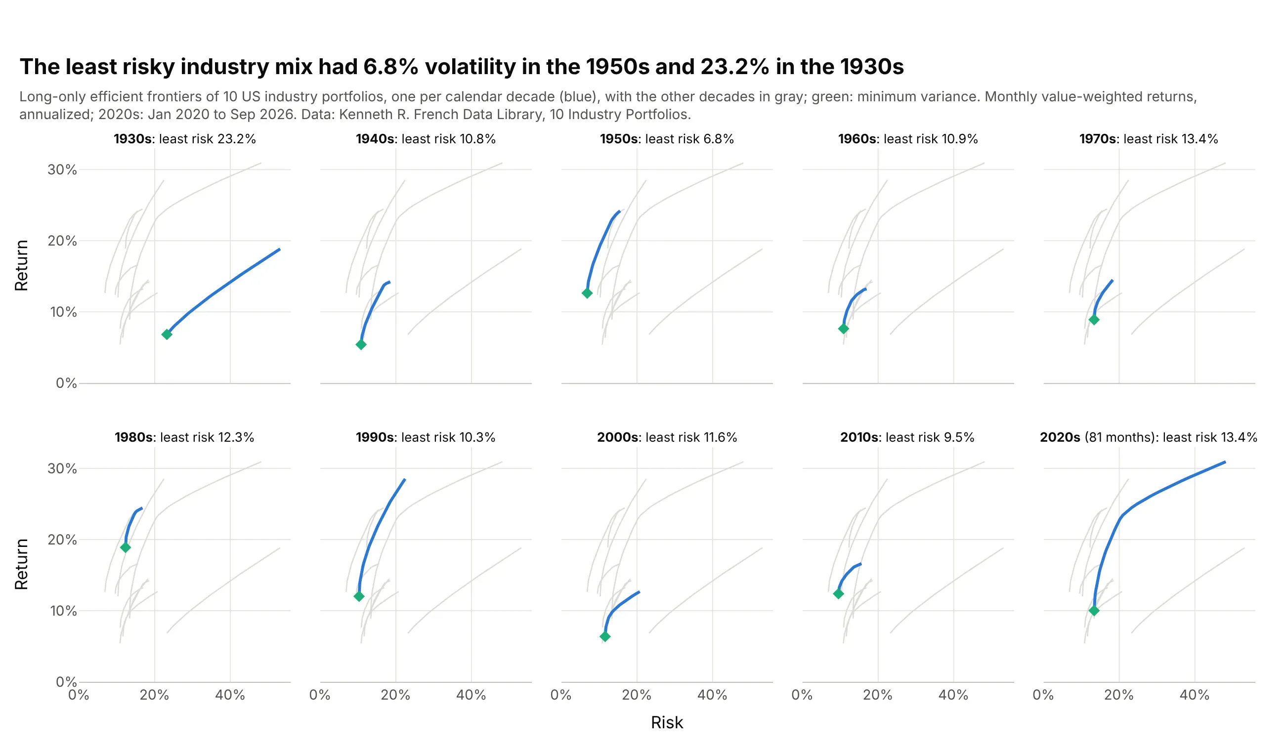
Ten small panels, one per decade from the 1930s to the 2020s, each showing that decade's long-only efficient frontier of 10 US industry portfolios in blue over the other nine decades in gray, with a green diamond for the minimum-variance portfolio: least risk 23.2% in the 1930s, 10.8% in the 1940s, 6.8% in the 1950s, 10.9% in the 1960s, 13.4% in the 1970s, 12.3% in the 1980s, 10.3% in the 1990s, 11.6% in the 2000s, 9.5% in the 2010s and 13.4% in the 2020s (81 months)

The least risky mix of the same 10 industries had 23.2% volatility in the 1930s and 6.8% in the 1950s, so a frontier from one decade says little about the next. Data: Kenneth R. French Data Library, 10 Industry Portfolios, January 1930 to September 2026.

Tip: ten curves on one chart tangle, so use small multiples with every other decade in light gray behind the one in blue, as in our small multiples guide.

Get the data from the Kenneth R. French Data Library (10_Industry_Portfolios_CSV.zip, value-weighted monthly
returns) and shape it into a table (columns: month, then one column per industry) from January 1930.

Compute the long-only efficient frontier of each calendar decade and build a plotly figure with make_subplots(2, 5,
shared axes): in each panel that decade's frontier in blue with its minimum-variance point, and the others in gray.