Chris Parmer

October 24, 2026

Bump Charts - A Complete Guide

TL;DR

A bump chart shows rankings over time: one line per item, rank 1 at the top, and a line moves up or down when the item changes place.
Bump charts are also known as bumps charts, after the rowing races where they started, and are similar to slope charts.
Use one when the question is who is ahead and when the order changed (the largest banks, the costliest drugs, the top oil producers, a league table).
Use a line chart of the values instead when the order rarely changes or the size of the gaps matters, because ranks hide both.
You can make a bump chart with Plotly from go.Scatter lines on a reversed y axis, and any coding agent can write one in a minute.

What is a bump chart?

Bump charts look like this:

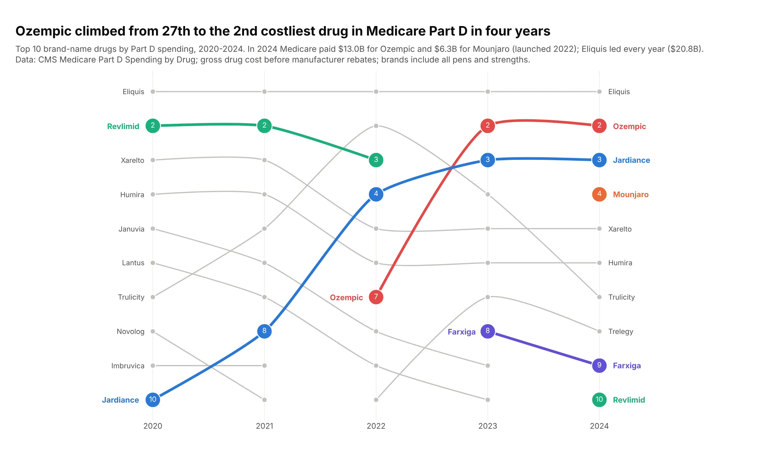
Data: CMS Medicare Part D Spending by Drug, 2020-2024, gross cost before rebates.

How do you read a bump chart? In the example above, notice these things:

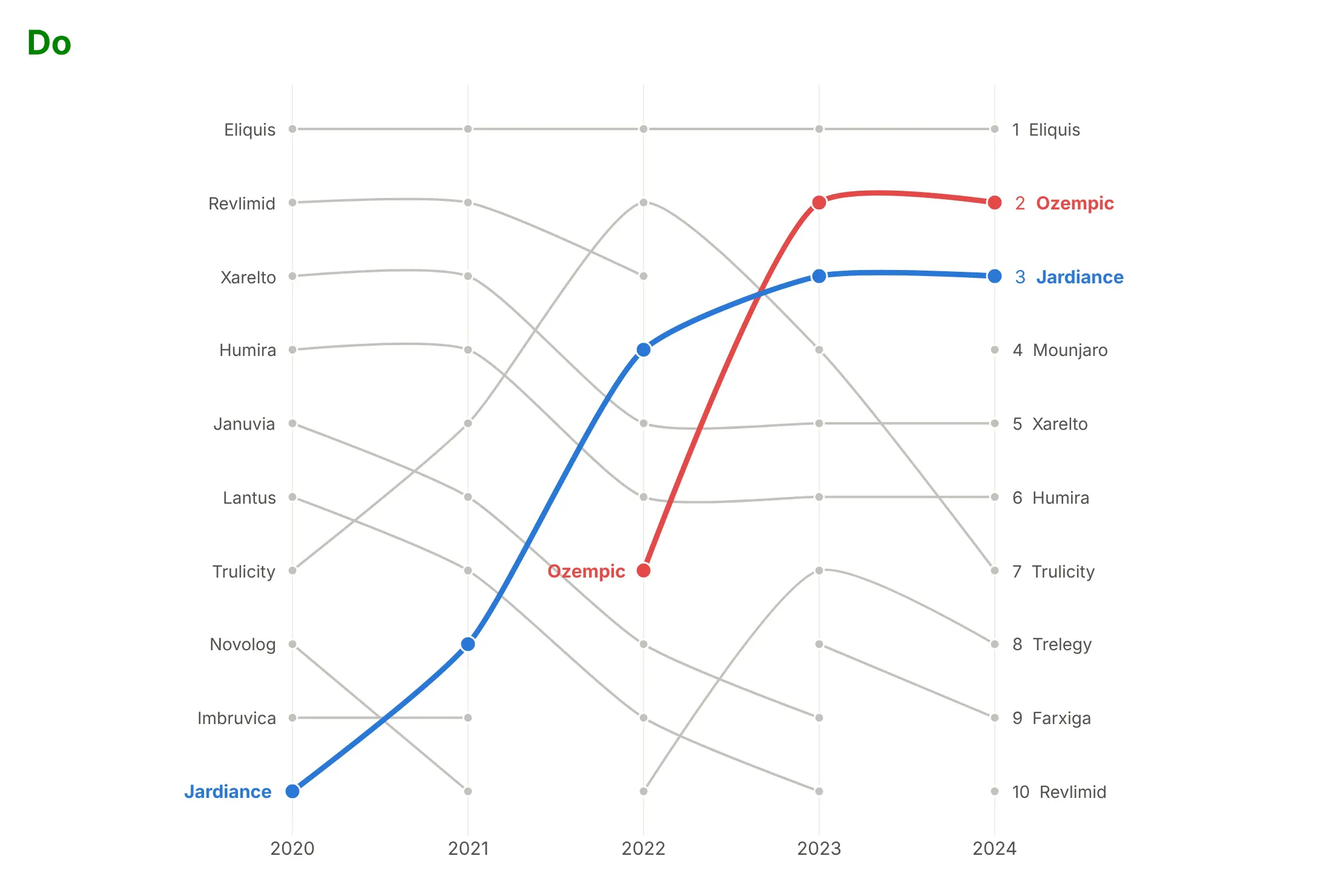
Each line is one drug, and its height in each year is its rank by Medicare Part D spending, with rank 1 at the top. Eliquis's flat gray line along the top row means it was the costliest drug in every year.
The height shows the rank and not the dollar amount, so every row is the same distance apart whatever the gap in spending. Eliquis and Ozempic sit on neighboring rows in 2024 even though Medicare spent far more on Eliquis.
Color picks out the drugs with a story, with their ranks printed in the markers, while the rest stay gray. Ozempic's red line makes the steepest climb in the chart, from 7th in 2022 to just below Eliquis a year later.
A line starts when a drug enters the top 10 and stops when it leaves. Ozempic's line only begins in 2022, and Mounjaro shows up as a single orange dot in the last year.
A break in a line doesn't mean the data is missing. Revlimid's green line stops after 2022 because it fell just below the top 10, and it comes back as a lone dot in 2024.

It's often used for charts like these:

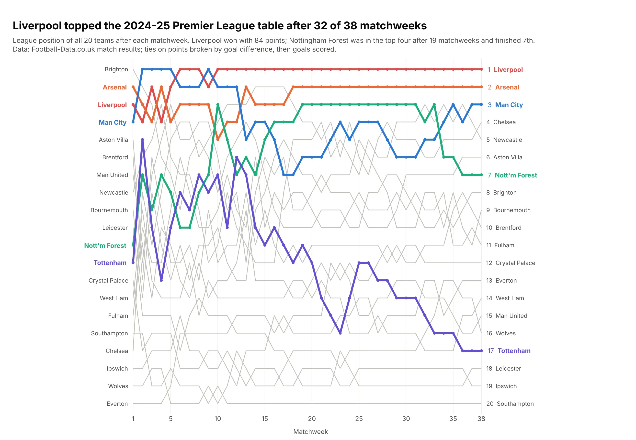
Bump chart of all 20 Premier League teams' positions after each of the 38 matchweeks of 2024-25. Liverpool leads from matchweek 10; Nottingham Forest spends 19 weeks in the top four and finishes 7th; Tottenham finishes 17th

A league table over a season. Liverpool topped the 2024-25 Premier League table after 32 of 38 matchweeks, and Nottingham Forest spent 19 matchweeks in the top four before finishing 7th. Data: Football-Data.co.uk match results.

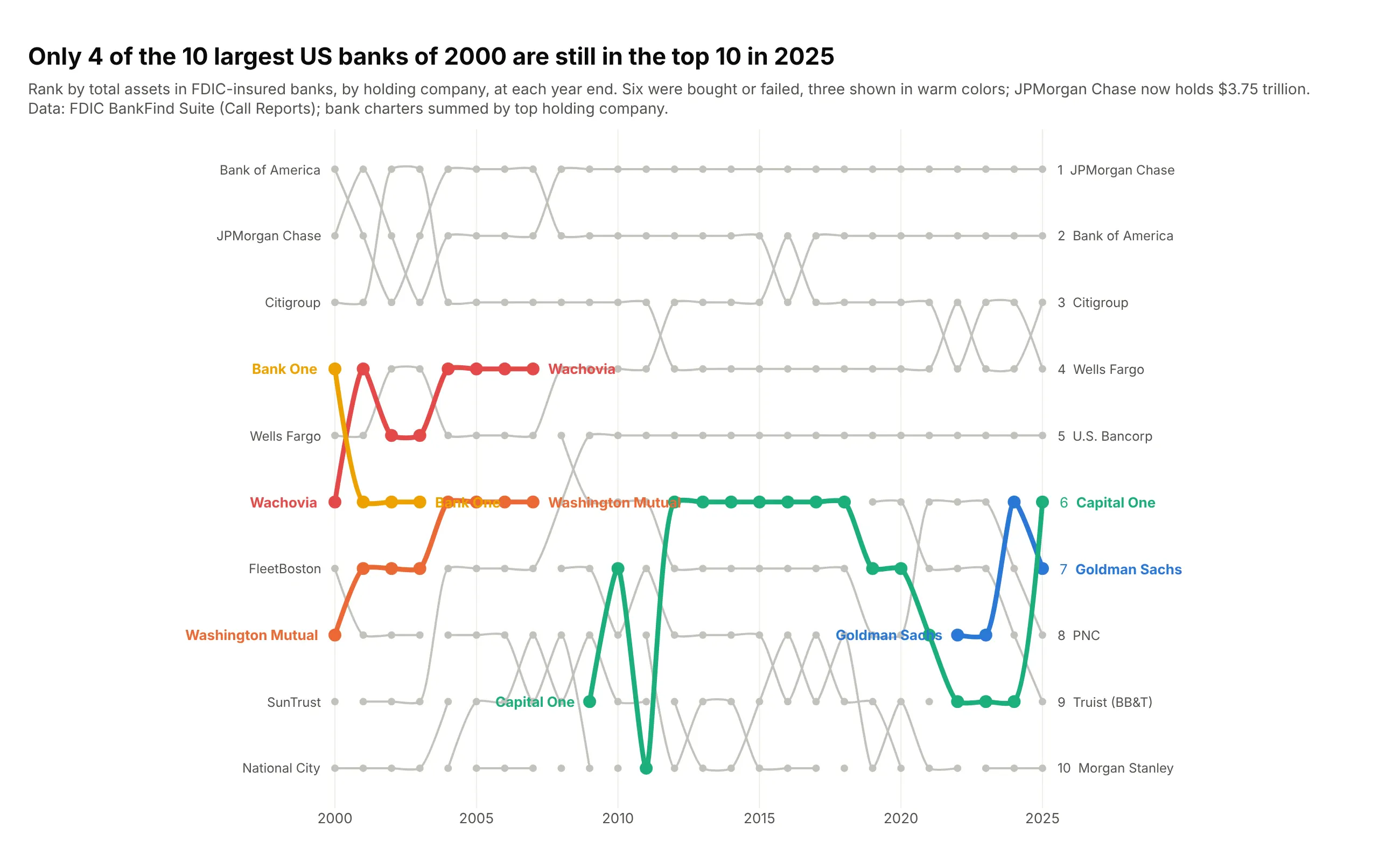
Bump chart of the 10 largest US bank holding companies by assets in FDIC-insured banks from 2000 to 2025. Wachovia, Washington Mutual and Bank One leave the chart; Capital One and Goldman Sachs arrive

A top 10 by year. Only 4 of the 10 largest US banks of 2000 were still in the top 10 at the end of 2025, because Wachovia, Washington Mutual, Bank One and three others were bought or failed. Data: FDIC BankFind Suite (Call Reports), summed by holding company.

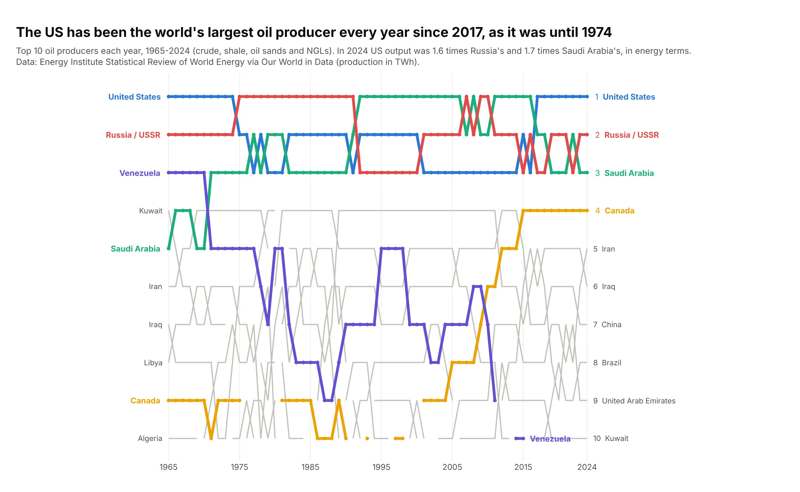
Bump chart of the 10 largest oil producers from 1965 to 2024. The US, the USSR/Russia and Saudi Arabia trade first place; Canada rises to 4th and Venezuela falls out

Countries ranked over decades. The US has been the world's largest oil producer every year since 2017, as it was until 1974, and Saudi Arabia and the USSR or Russia held first place in between. Data: Energy Institute Statistical Review of World Energy, via Our World in Data.

A short history

The name comes from rowing. Oxford's college bumping races go back to 1815 and Cambridge's bumping races to 1827: crews start in a line, one behind the other, and try to catch and bump the boat ahead, which earns them its place for the next day. The results have long been drawn as a chart of every crew's position day by day, which is the layout bump charts still use:

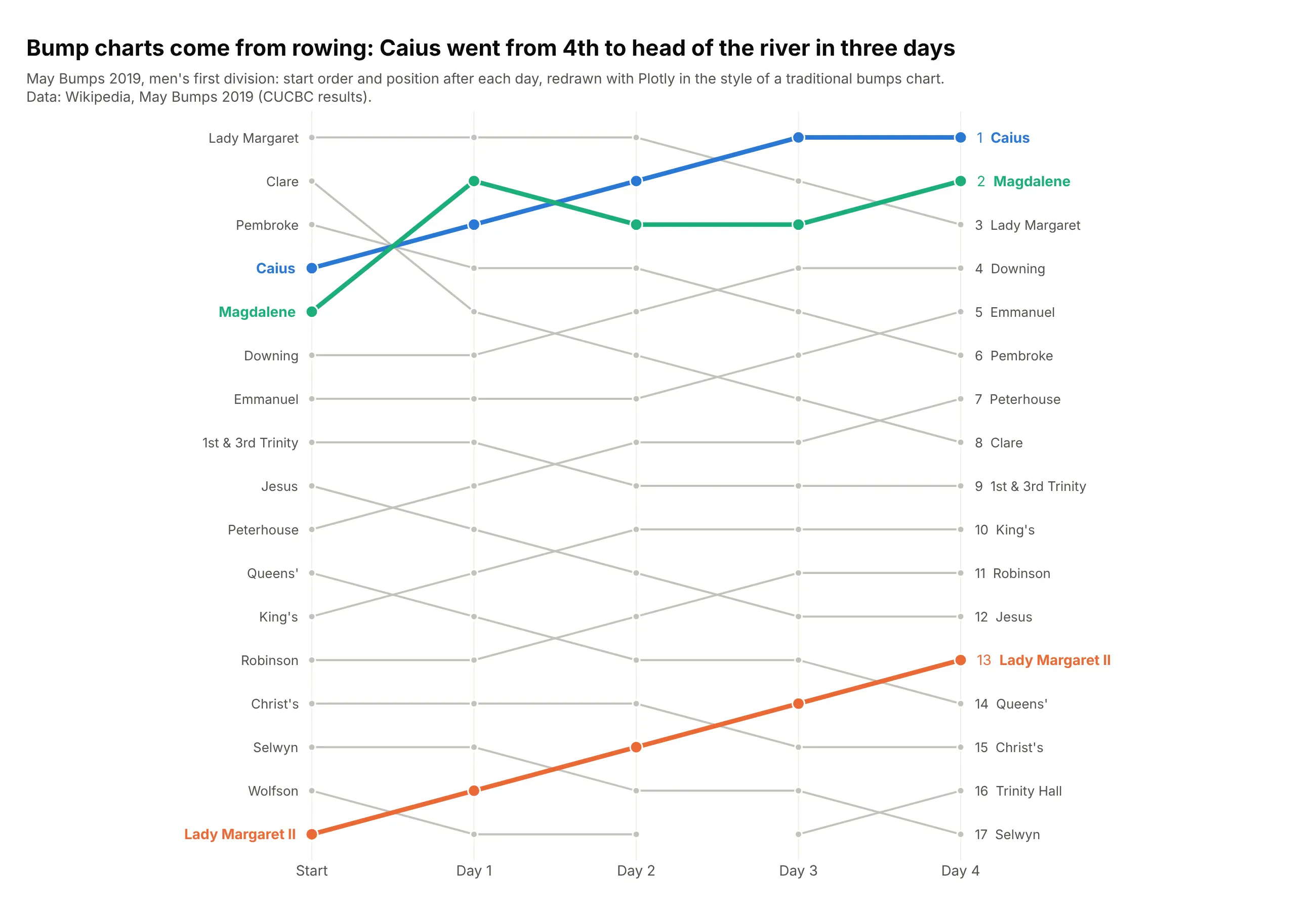
A traditional bumps chart redrawn with Plotly: the 17 crews of the men's first division of the 2019 May Bumps, from the start order to the position after each of four days. Caius rises from 4th to 1st by day 3, Magdalene from 5th to 2nd, and Lady Margaret II from 17th to 13th by bumping once a day

Caius started 4th in the 2019 May Bumps and bumped Pembroke, Magdalene and Lady Margaret on the first three days to finish head of the river. The same chart became the standard way to show league tables over a season, and in data visualization it's a close relative of the slope chart, which keeps only the first and last dates.

Alternatives to a bump chart

Here's the same drug ranking drawn six ways. Some are better for the question, some worse, some just different:

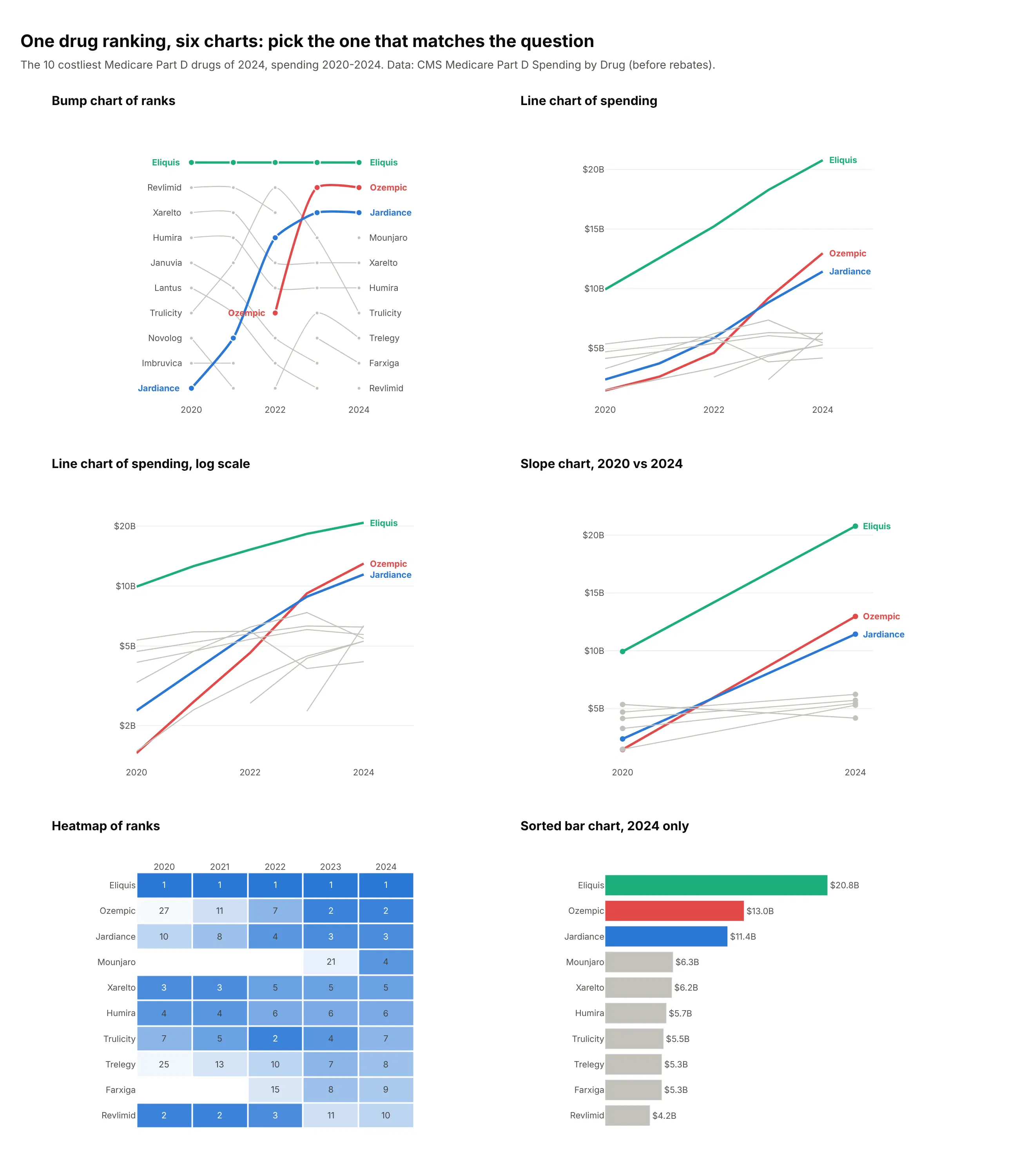
The 10 costliest Medicare Part D drugs of 2024 drawn six ways: a bump chart of ranks, a line chart of spending, a line chart of spending on a log scale, a slope chart of 2020 vs 2024 spending, a heatmap of ranks with Ozempic going from 27th to 2nd, and a sorted bar chart of 2024 spending led by Eliquis at $20.8B

Line chart of the values (better when the gaps matter). It shows that Eliquis's $20.8B in 2024 was well ahead of Ozempic's $13.0B, a gap the ranks hide. Position on a common scale is the most accurate visual encoding people have (Cleveland and McGill, 1984), and a bump chart spends it on the rank, so a 0.1% gap and a 50% gap look the same.
Line chart on a log scale (different). Equal slopes mean equal growth rates, so it shows how fast Ozempic grew, but readers have to work harder to compare levels.
Slope chart (works too, for two dates). It keeps only the start and the end, which is clearer when that's the comparison and hides everything in between. See our slope chart guide.
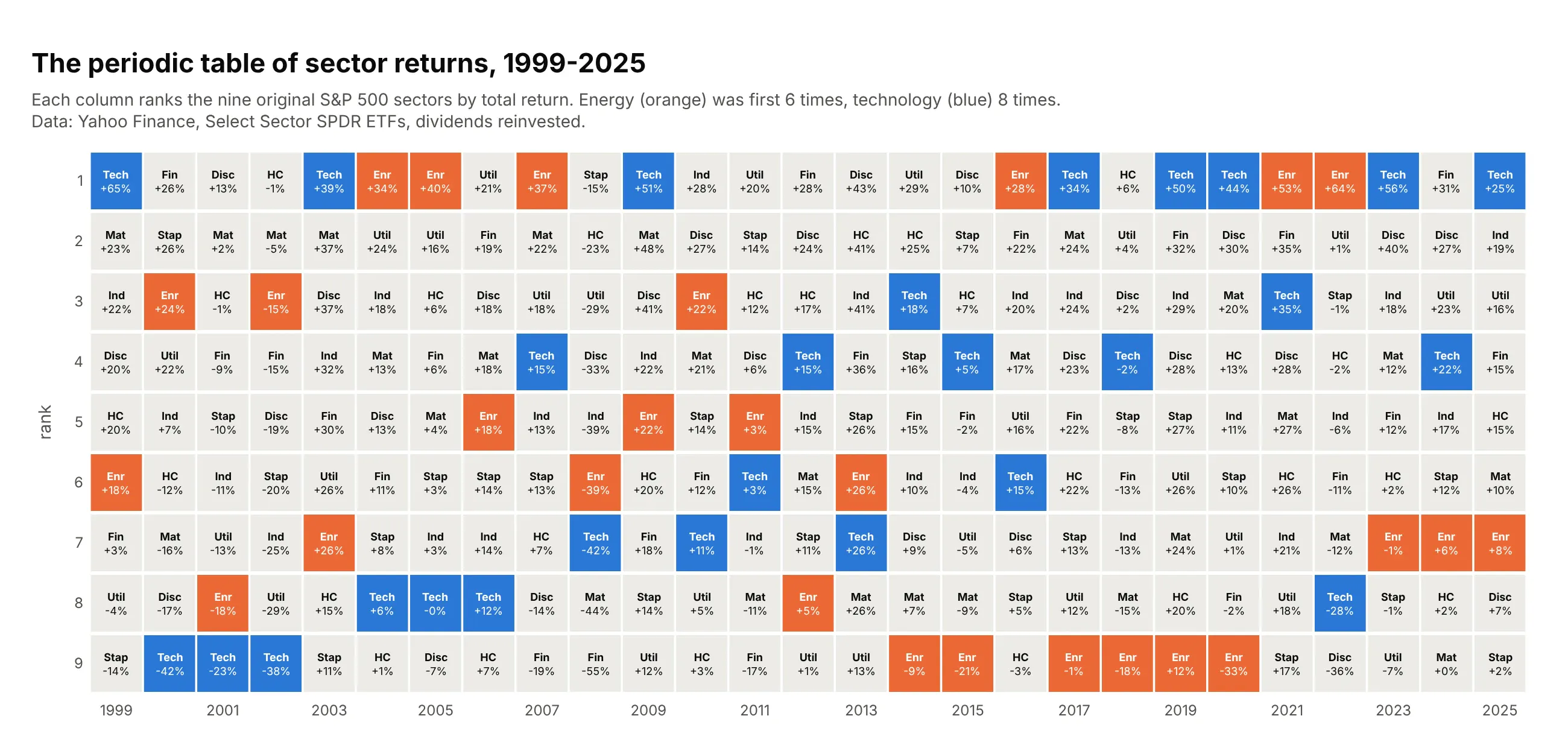
Heatmap of ranks (works too). The "periodic table of returns" in finance prints the exact rank in every cell, including ranks below the cut, but readers have to follow an item by its row instead of a line. See our heatmap guide.
Sorted bar chart (better for one date). When the question is only about the latest ranking, bars compare the values precisely and need no time axis.

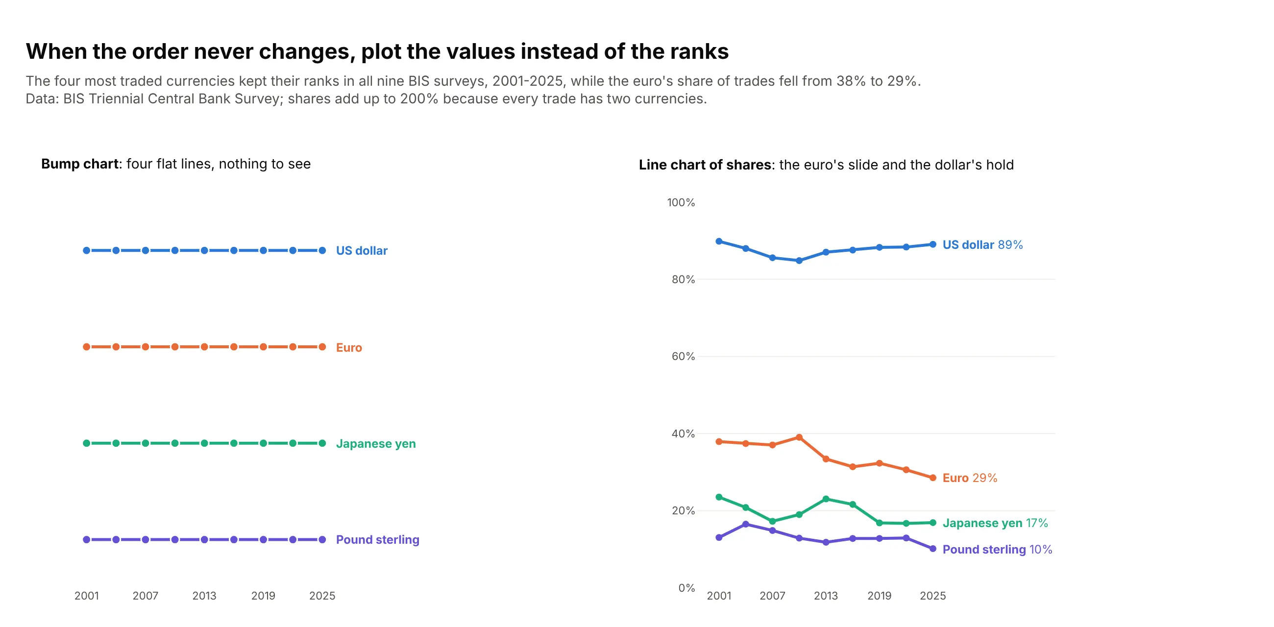
Here's where the line chart wins. The four most traded currencies kept their ranks in all nine surveys since 2001, so the bump chart is four flat lines, while the shares show the euro falling from 38% to 29% of trades:

The four most traded currencies as a bump chart (four flat lines) and as a line chart of their share of trading, where the euro falls from 38% to 29%

How to make a bump chart

With AI

ChatGPT, Claude Code, GitHub Copilot, Cursor and other AI tools are excellent at writing Plotly code. Name Plotly in the prompt, say how to rank and what to highlight, and list the checks you want:

Make a plotly bump chart from rankings.csv (columns: year, company, revenue_usd_bn).

- Rank companies by revenue within each year (1 = largest) with rank(method="first"),
  on all rows, then show the top 10.
- One go.Scatter trace per company, mode lines+markers, y axis range [10.5, 0.5]
  so rank 1 is at the top, no y tick labels.
- Break a line when a company is outside the top 10 (NaN, connectgaps=False).
- Highlight Eli Lilly and Novo Nordisk in #e34948 and #2a78d6; all others #c3c2bc,
  drawn first so the highlights sit on top.
- Labels at both ends as annotations, final rank before the right-hand label, no legend.
- A title that states the main takeaway with the ranks.
- Print any company whose rank changes by more than 5 places in one year, so I can check it.
- Save it as bump.html and as a PNG at 2x scale.

The last check catches the most common bump chart bug: a renamed or merged company that shows up as one line falling out and another jumping in.

With Plotly Studio

Plotly Studio is a desktop app where you point an AI at a dataset and it builds charts and a Dash app around your questions. Ask for a bump chart by saying what to rank and what to highlight:

Rank the drugs by Medicare Part D spending in each year and show the top 10 as a bump chart, with rank 1 at the top, Ozempic and Jardiance in color and every other drug in gray, labels at both ends instead of a legend, and a dropdown to pick which drugs to highlight.

Make a bump chart in Python or JavaScript

This is the code AI tools write under the hood. In Python, this short helper draws one go.Scatter line per item on a reversed y axis, with gray context lines, a few highlights, labels at both ends and breaks when an item leaves the top N:

import pandas as pd
import plotly.graph_objects as go


def make_bump(df, x, entity, rank, top_n=10, highlight=(), spline=True):
    """One line per entity, rank 1 at the top, labels at both ends, gray context."""
    palette = ["#2a78d6", "#eb6834", "#1baf7a", "#eda100", "#6250d6"]
    colors = {e: palette[i % len(palette)] for i, e in enumerate(highlight)}
    xs = sorted(df[x].unique())
    shown = df.loc[df[rank] <= top_n, entity].unique()
    fig = go.Figure()
    for e in sorted(shown, key=lambda e: e in colors):  # highlighted lines drawn last, on top
        r = df[df[entity] == e].set_index(x)[rank].reindex(xs)
        r = r.where(r <= top_n)  # NaN breaks the line while the entity is outside the top N
        c = colors.get(e, "#c3c2bc")
        fig.add_trace(go.Scatter(
            x=xs, y=r, name=e, mode="lines+markers", connectgaps=False,
            line=dict(color=c, width=4 if e in colors else 2, shape="spline" if spline else "linear"),
            marker=dict(color=c, size=10 if e in colors else 6),
        ))
        for i, side, shift in ((0, "right", -10), (-1, "left", 10)):  # labels instead of a legend
            if pd.notna(r.iloc[i]):
                fig.add_annotation(x=xs[i], y=r.iloc[i], text=e, xanchor=side, xshift=shift,
                                   showarrow=False, font=dict(color=c if e in colors else "#52514e"))
    fig.update_yaxes(range=[top_n + 0.5, 0.5], visible=False)  # rank 1 at the top
    fig.update_xaxes(tickvals=xs, showgrid=False)
    fig.update_layout(showlegend=False, plot_bgcolor="white", margin=dict(l=150, r=150))
    return fig


df = pd.read_csv("part_d.csv")  # columns: year, brand, spending_bn, rank
make_bump(df, "year", "brand", "rank", top_n=10, highlight=["Ozempic", "Jardiance"]).show()

Keep more rows than you plot (the top 20 or 30 when you show a top 10), so the helper knows where an item was before it entered. For a quick draft, px.line(df, x="year", y="rank", color="brand", markers=True) followed by fig.update_yaxes(autorange="reversed") is enough.

In JavaScript, plotly.js builds the same chart from one scatter trace per item, here five drugs ranked by Medicare Part D spending:

<div id="chart"></div>
<script src="https://cdn.plot.ly/plotly-4.1.1.min.js"></script>
<script>
  const years = [2022, 2023, 2024];
  const ranks = {  // rank by Part D spending among these five drugs
    Eliquis: [1, 1, 1], Ozempic: [5, 2, 2], Jardiance: [3, 3, 3],
    Xarelto: [4, 5, 4], Trulicity: [2, 4, 5]
  };
  const colors = { Ozempic: "#e34948", Jardiance: "#2a78d6" };
  const names = Object.keys(ranks).sort((a, b) => (a in colors) - (b in colors));
  Plotly.newPlot("chart", names.map(name => ({
    type: "scatter", mode: "lines+markers+text", x: years, y: ranks[name], name,
    text: ["", "", name], textposition: "middle right", cliponaxis: false,
    line: { shape: "spline", width: name in colors ? 4 : 2, color: colors[name] || "#c3c2bc" },
    marker: { size: name in colors ? 10 : 6, color: colors[name] || "#c3c2bc" }
  })), {
    yaxis: { range: [5.5, 0.5], visible: false },  // rank 1 at the top
    xaxis: { tickvals: years },
    showlegend: false, margin: { r: 100 }
  });
</script>

Share it

Every Plotly chart has a Share chart button (the cloud icon in its toolbar) that uploads it to Plotly Cloud and gives you a link. Only you can see it until you change its visibility.

For a live app, put the chart in a Dash app and publish it with the Plotly Cloud CLI. Coding agents can run these commands for you:

pip install "dash[cloud]"
plotly user login
plotly app publish

If your data has to stay in your own cloud or data center, publish to Dash Enterprise instead.

Dos and don'ts

Plotting rank as a plain line chart puts rank 1 at the bottom, connects every point and adds a legend, so most of the work is undoing that and choosing what to leave out. Here is the same Medicare Part D ranking both ways.

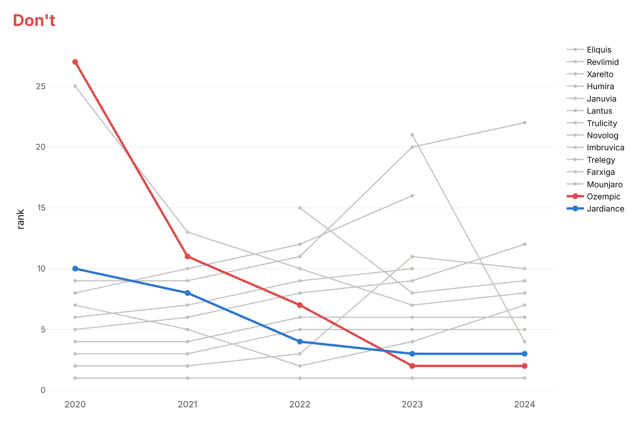
Don't leave rank 1 at the bottom, connect lines through ranks below the cut (here Ozempic's 27th place in 2020 squeezes the top 10 into the bottom of the chart and makes its climb look like a fall) or make readers match 14 lines to a legend:

The Medicare Part D ranking with Ozempic in red, Jardiance in blue and the other drugs in gray, but with rank 1 at the bottom, lines connected through ranks down to 27th so the top 10 fills only the lower part of the chart, and a legend instead of labels on the lines

Do use the same colors, reverse the axis, label both ends and break lines where a drug is outside the top 10:

The same ranking as a bump chart: rank 1 at the top, Ozempic in red entering at 7th in 2022 and reaching 2nd, Jardiance in blue rising from 10th to 3rd, the other drugs in gray, labels at both ends and breaks where drugs leave the top 10

Use color for the story

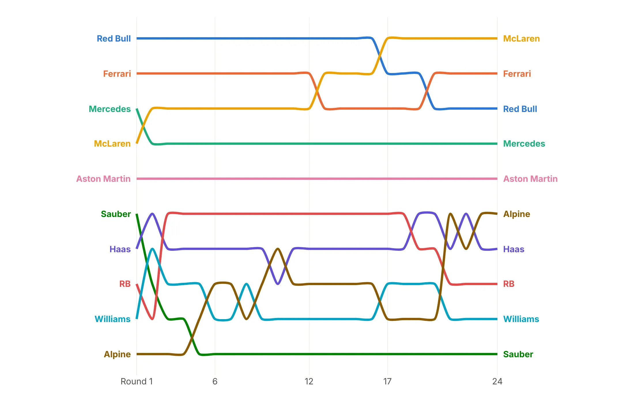
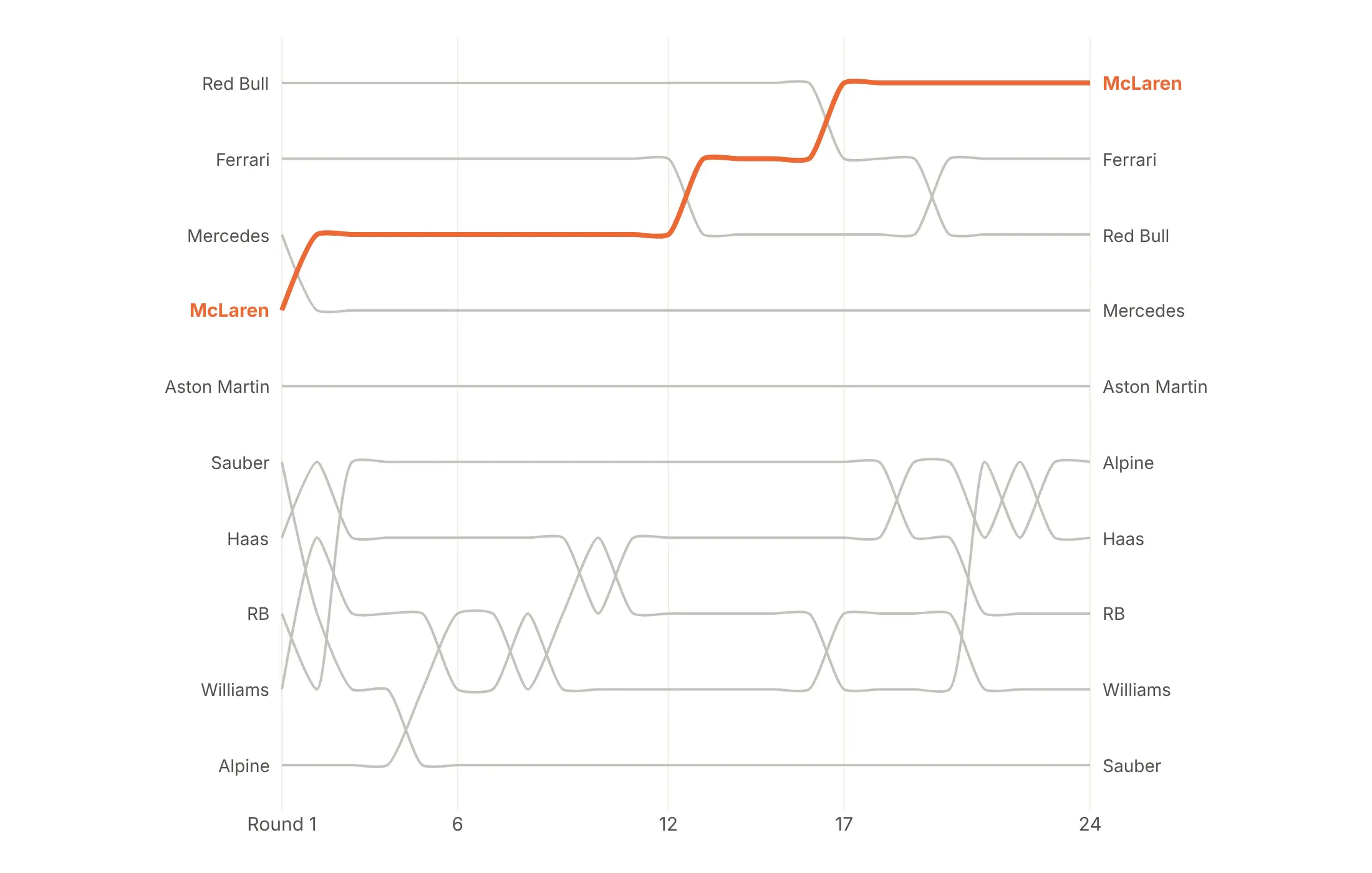
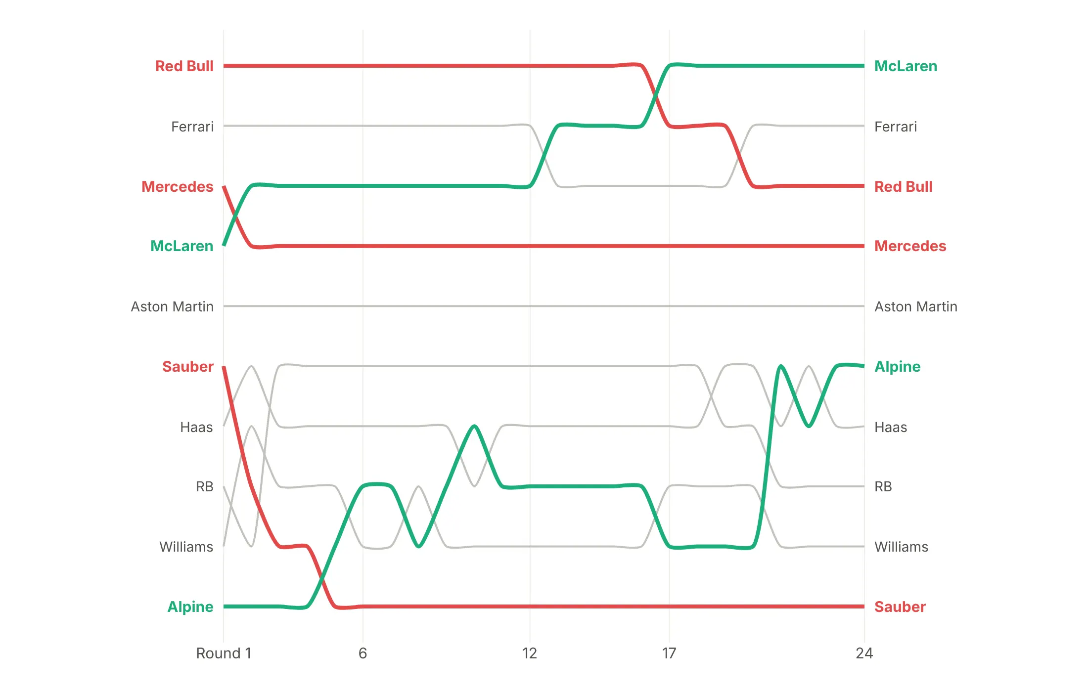
Color is the main decision in a bump chart. Here are four options on the 2024 Formula 1 constructors' standings after each of 24 rounds.

Every line in its own color (avoid). This is what a default palette does, and with ten colors nothing stands out.

The 2024 F1 constructors' standings as a bump chart with each of the ten teams in its own color

One story in color. McLaren started 4th and took the lead from Red Bull after round 17, so it's the only color and every other team is gray.

The 2024 F1 constructors' standings with McLaren in orange climbing from 4th to 1st and every other team in gray

A group in color. The three teams in the title fight (McLaren, Ferrari and Red Bull) get colors, which shows how they traded places.

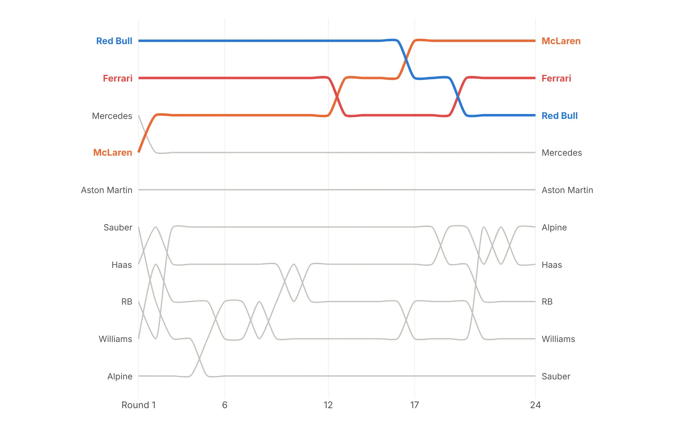
The 2024 F1 constructors' standings with McLaren, Ferrari and Red Bull in color and the other seven teams in gray

Color by direction. Teams that finished higher than after round 1 are green and those that finished lower are red, such as Alpine climbing from 10th to 6th.

The 2024 F1 constructors' standings with McLaren and Alpine in green for finishing higher than they started, Red Bull, Mercedes and Sauber in red for finishing lower, and the rest in gray

Checklist

Reverse the y axis so rank 1 is at the top (range=[N + 0.5, 0.5] or autorange="reversed").
Color two to five lines and draw the rest in light gray, with the highlighted lines drawn last so they sit on top.
Label both ends with annotations, and put the final rank in front of the right-hand label.
Break lines at the cut with connectgaps=False, and label where a highlighted line leaves or enters.
Print the rank inside large markers when there are only five or six periods.
Write a title that states the takeaway with the ranks, such as "rose from 8th to 2nd".

Don't

Leave rank 1 at the bottom, because every reader expects first place at the top.
Connect lines across gaps, since a line from 9th in 2000 to 8th in 2004 implies four years in the top 10 that didn't happen.
Use a legend when you can label the lines.
Smooth dense data with splines, which can overshoot past a row when many swaps happen in a row.

Options to customize

Plotly builds a bump chart from go.Scatter traces and the layout, so these are the options that matter most. The full reference is in the Plotly line chart documentation.

go.Scatter(x, y) with y = rank: one trace per item; px.line(color=...) makes a quick draft.
mode: "lines+markers" for highlighted lines, "lines" for dense gray context.
yaxis.range=[N + 0.5, 0.5] or autorange="reversed": puts rank 1 at the top.
yaxis.tickvals, showticklabels: rank numbers on the axis; hide them when the labels carry the rank.
connectgaps=False with NaN ranks: breaks a line while an item is outside the top N.
line.shape="spline", line.smoothing: curved lines, for up to about 20 periods with occasional swaps.
line.width, line.color: thick colored highlights and thin gray context.
marker.size, marker.line: big markers with a white outline, for printing the rank inside.
go.Scatter(mode="text"): rank numbers on top of the markers.
layout.annotations (xanchor, xshift): labels at both ends instead of a legend.
showlegend=False: removes the legend once the lines are labeled.
hovertemplate, customdata: the value behind the rank in the hover.
xaxis.tickvals, ticktext: name rounds or races on the time axis.
None separators in one trace: many gray context lines in a single trace, which draws faster.

More bump chart examples

Ten more bump charts built from real public data, each with its source, the technique that makes it work and a prompt to rebuild it.

1. S&P 500 sectors ranked by return each year

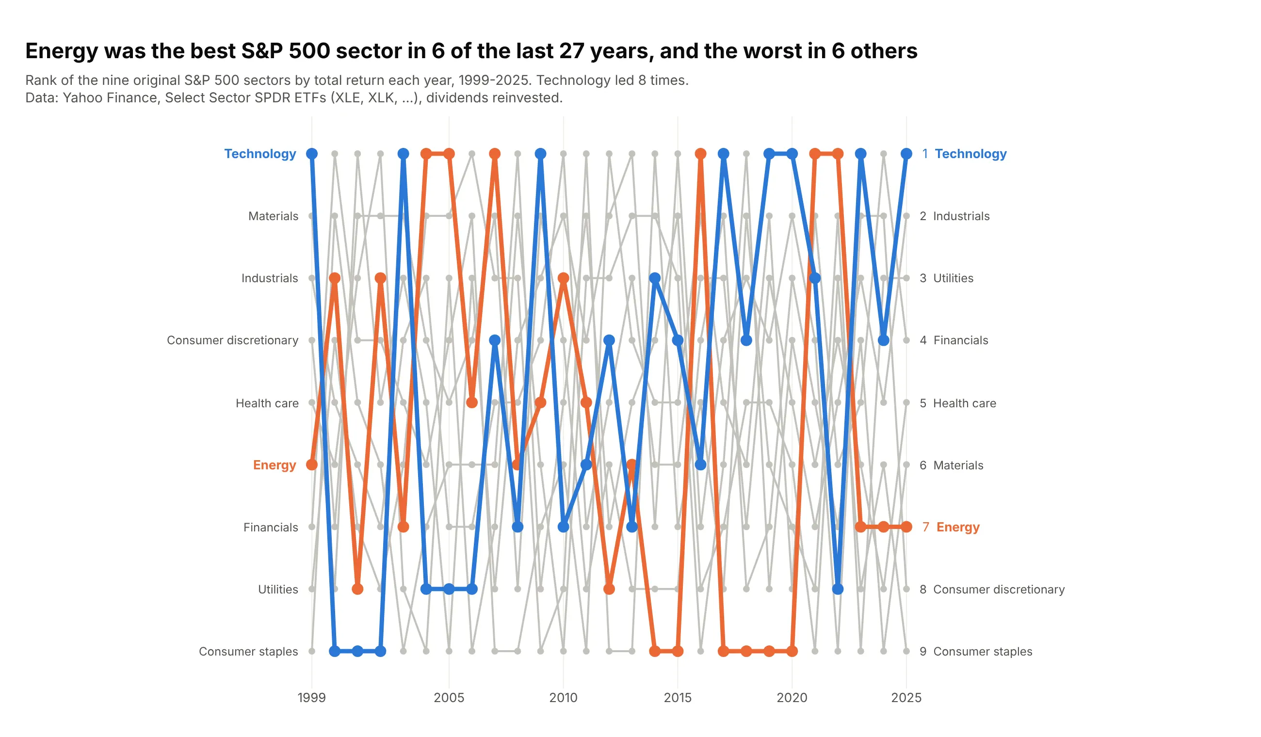
Bump chart of the nine original S&P 500 sectors ranked by total return each year from 1999 to 2025, with energy and technology highlighted. Energy was first in 6 years and last in 6 others; technology was first 8 times

Energy was the best of the nine original S&P 500 sectors in 6 of the 27 years from 1999 to 2025, and the worst in 6 others. It returned +64% in 2022 and -33% in 2020. Data: Yahoo Finance, Select Sector SPDR ETFs, dividends reinvested.

Tip: with every sector on the chart and 27 dense columns, use straight lines (spline=False), because splines overshoot past rank 1 and rank 9.

Get the data from Yahoo Finance: daily adjusted closes for the nine Select Sector SPDR ETFs
(XLB, XLE, XLF, XLI, XLK, XLP, XLU, XLV, XLY) from December 1998 to December 2025, and compute
yearly total returns (columns: year, ticker, sector, total_return).

Build a plotly bump chart of the sectors ranked by total_return each year (1 = best), 1999-2025.
- All nine sectors shown, straight lines, rank 1 at the top.
- Energy in #eb6834 and Technology in #2a78d6, everything else gray.
- Labels at both ends, hover shows the return.
- Title: how many times energy was first and last.

Another way to see it: a heatmap of ranks, the "periodic table of returns", prints every sector's return in its cell.

Heatmap of the nine sectors' ranks by year from 1999 to 2025 with each cell labeled by sector and return; energy cells in orange and technology in blue

2. The largest economies

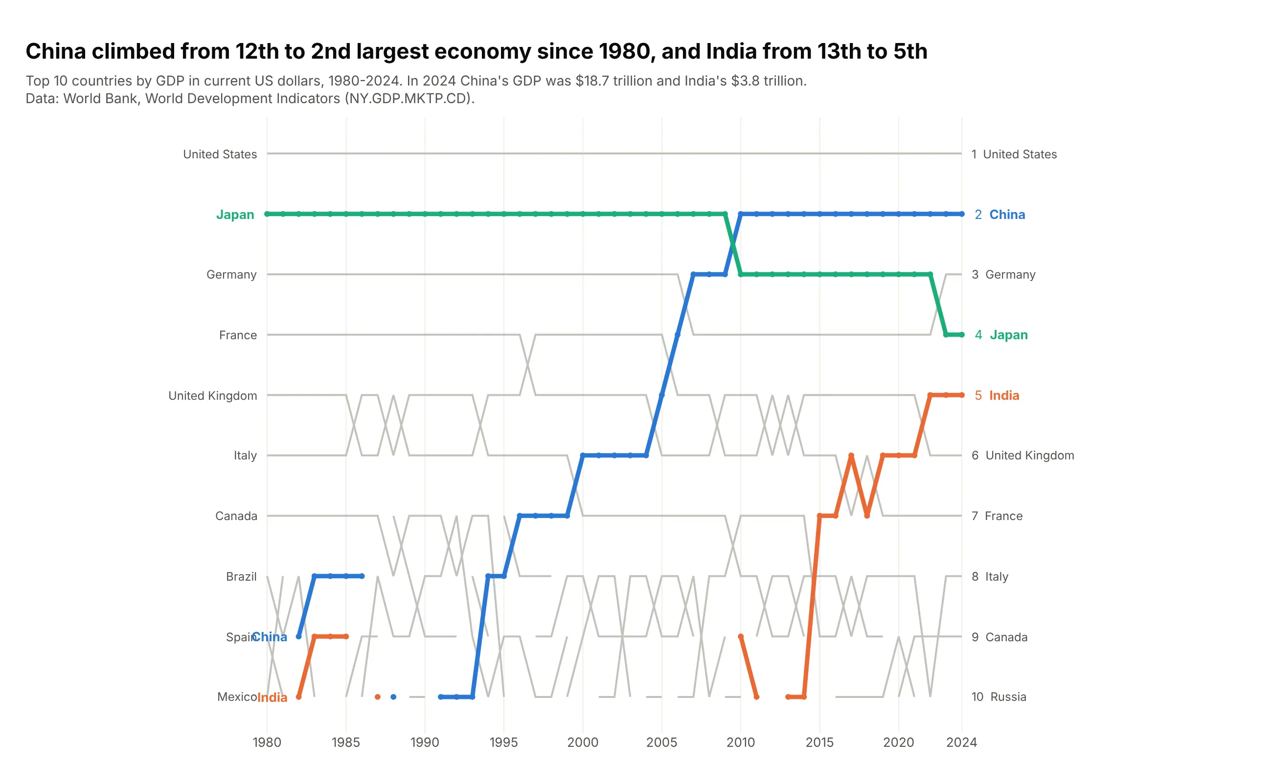
Bump chart of the 10 largest economies by GDP in current US dollars from 1980 to 2024, with China climbing from 12th to 2nd, India from 13th to 5th and Japan falling from 2nd to 4th

China climbed from the 12th largest economy in 1980 to 2nd in 2010, and India from 13th to 5th by 2022. Japan, 2nd for three decades, is now 4th. Data: World Bank, World Development Indicators (GDP, current US$).

Tip: hide markers on the gray lines (sizes=(0, 6)), since 45 markers per line read as a dashed line.

Get the data from the World Bank's World Development Indicators API, indicator NY.GDP.MKTP.CD
(GDP in current US$) for all countries, 1980-2024, without regional aggregates
(columns: year, iso3, country, gdp_bn, rank).

Build a plotly bump chart of the top 10 economies each year.
- Keep the top 20 so China and India enter from below the cut.
- China, India and Japan in color; straight lines; no markers on gray lines.
- Title with China's and India's ranks in 1980 and 2024.

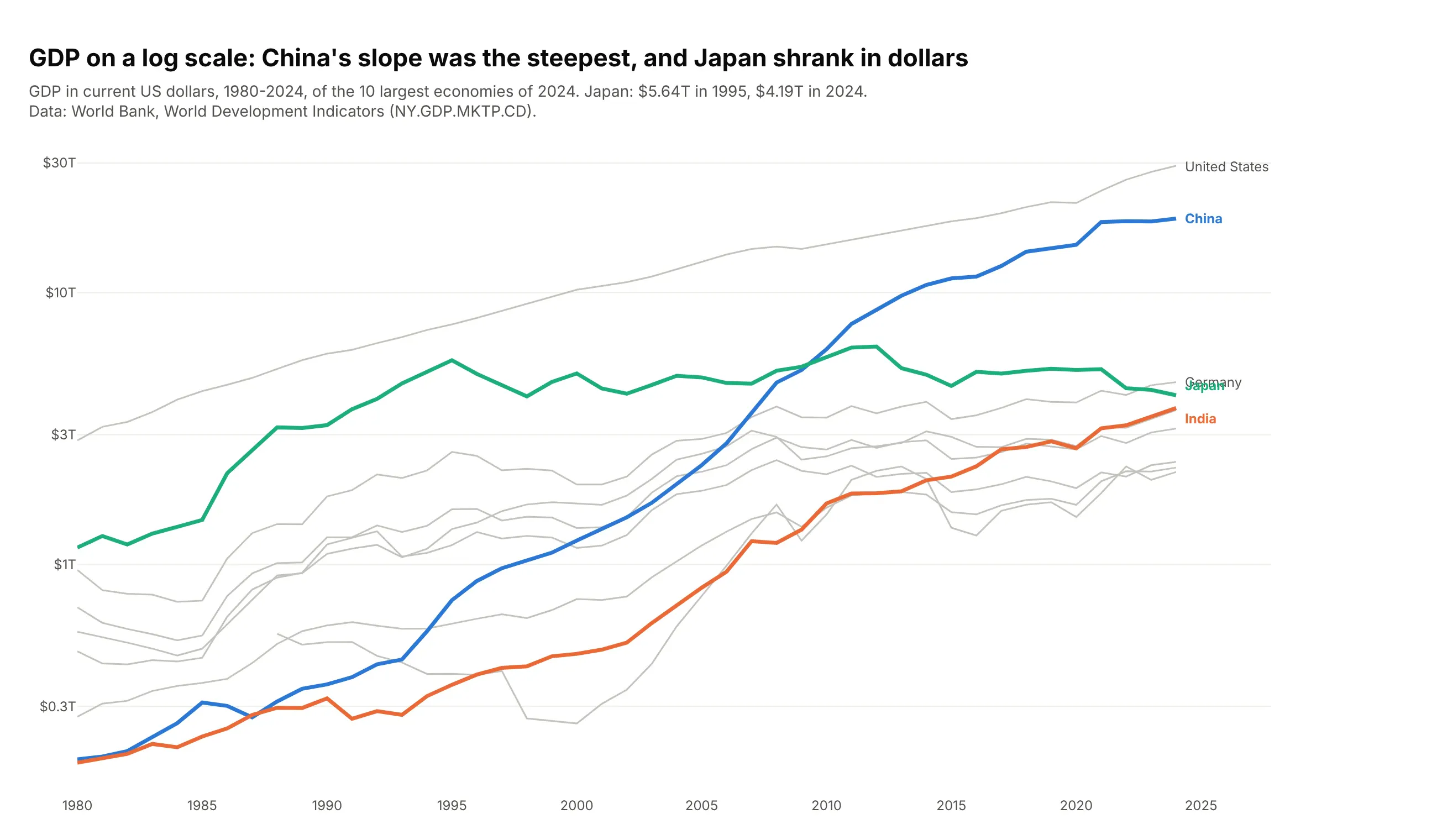
Another way to see it: GDP on a log scale shows growth rates as slopes, and that Japan's GDP in dollars fell from $5.64 trillion in 1995 to $4.19 trillion in 2024.

Line chart of GDP on a log scale for the 10 largest economies of 2024, 1980-2024, with China's line rising steeply and Japan's flat since 1995

3. The renminbi's climb in currency trading

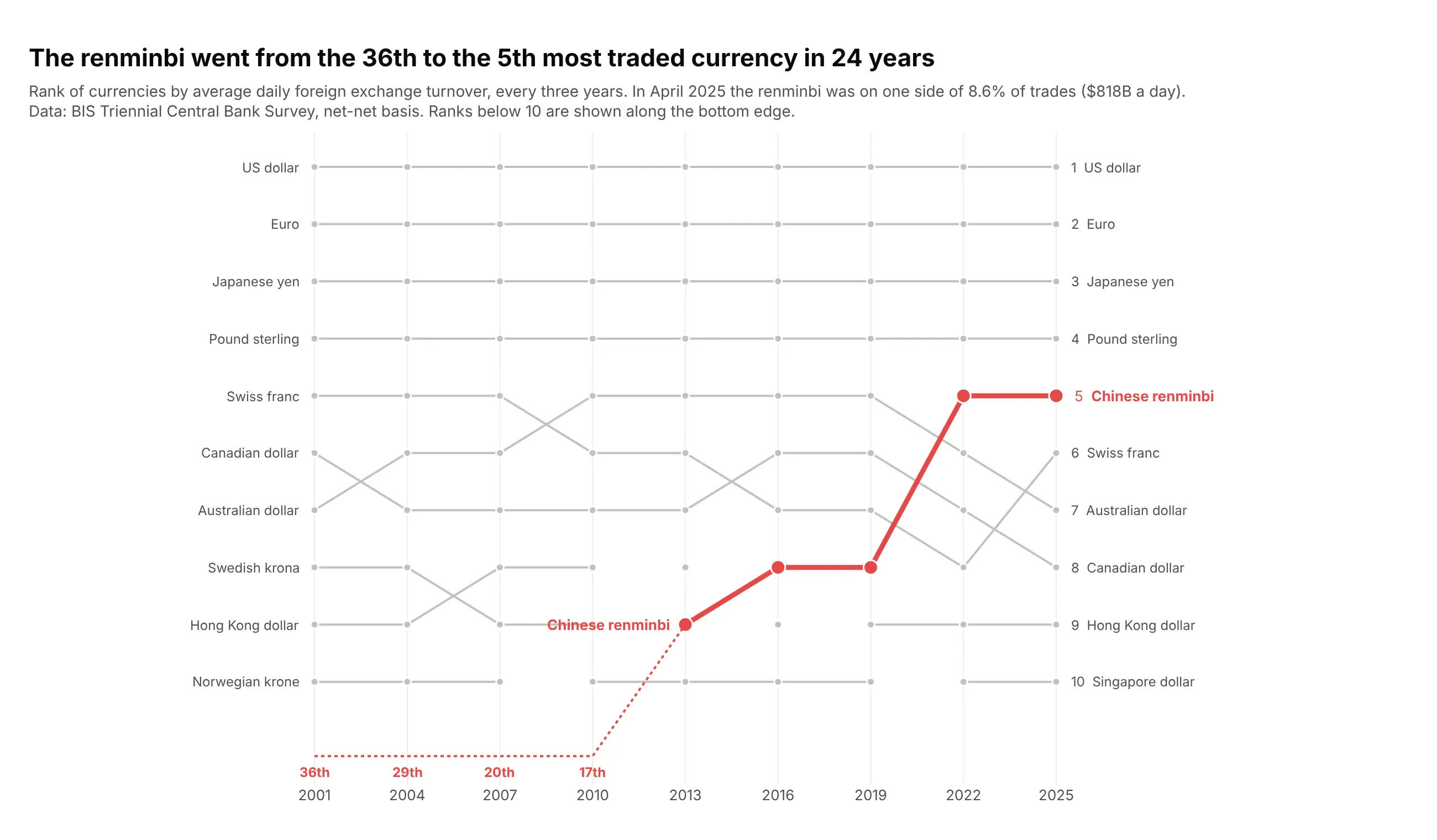
Bump chart of the 10 most traded currencies in nine BIS surveys from 2001 to 2025. The renminbi climbs from 36th to 5th, shown with a dotted line along the bottom edge while it was below the top 10

The Chinese renminbi went from the 36th most traded currency in 2001 to 5th in 2022 and 2025. In April 2025 it was on one side of 8.6% of all trades, $818B a day. Data: BIS Triennial Central Bank Survey.

Tip: when the story starts below the cut, draw it along the bottom edge with a dotted line and print the ranks there.

Get the data from the BIS Triennial Central Bank Survey (stats.bis.org, dataset WS_DER_OTC_TOV,
FX turnover by currency, net-net basis, April of each survey, 2001-2025)
(columns: year, code, currency, turnover_bn, share_pct, rank).

Build a plotly bump chart of the top 10 currencies per survey.
- Highlight the renminbi in red; straight lines.
- For surveys where it ranked below 10, draw a dotted segment along the bottom edge and
  print its rank under each point.

4. US electricity by source

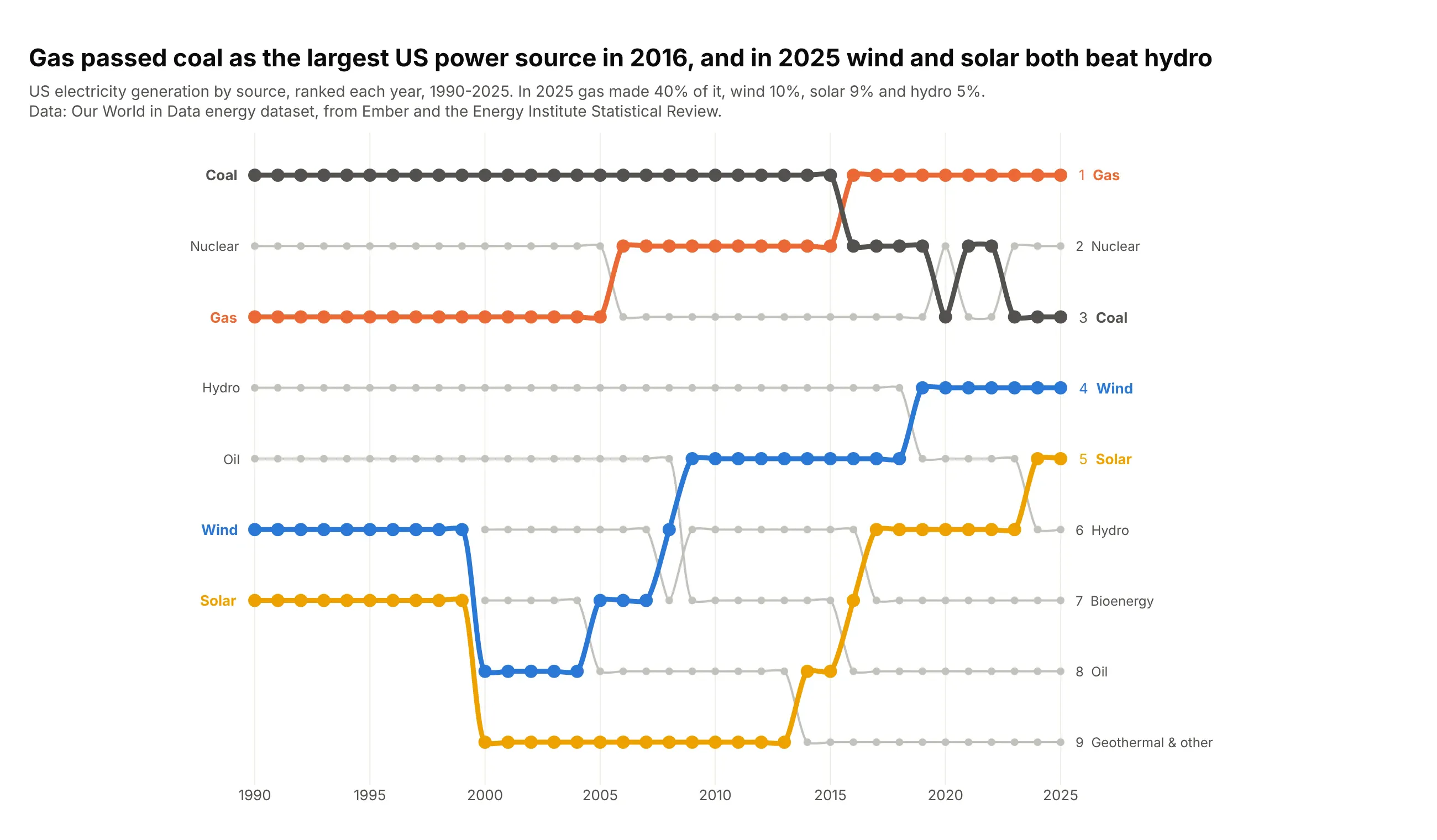
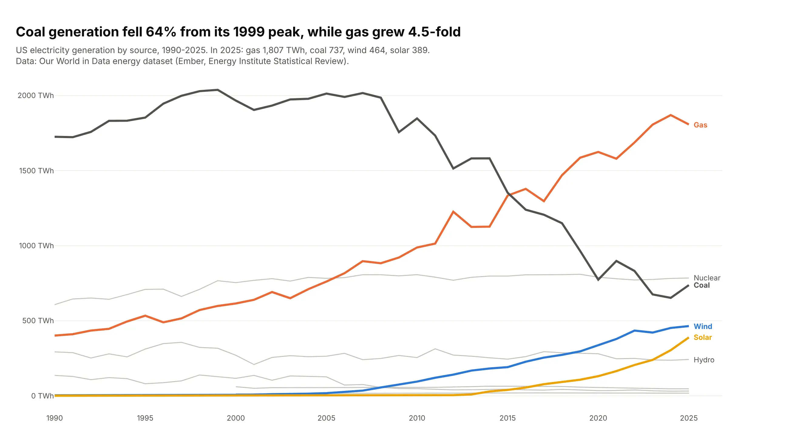
Bump chart of nine US electricity sources ranked by generation from 1990 to 2025. Gas passes coal in 2016; wind passes hydro in 2019 and solar in 2024

Gas passed coal as the largest US power source in 2016, and in 2025 wind (10%) and solar (9%) both generated more than hydro (5%). Gas made 40% of US electricity in 2025. Data: Our World in Data energy dataset (Ember, Energy Institute).

Tip: splines work here because the sources change places rarely and by one or two rows.

Get the data from Our World in Data's energy dataset (owid-energy-data.csv, from Ember and the
Energy Institute), United States, 1990-2025, generation by source in TWh
(columns: year, source, twh, share_pct, rank).

Build a plotly bump chart of the nine sources ranked by generation each year.
- Gas, coal, wind and solar in color, others gray; spline lines.
- Title: the year gas passed coal and what wind and solar passed in 2025.

Another way to see it: the values show that coal fell 64% from its 1999 peak while gas grew 4.5-fold since 1990.

Line chart of US electricity generation by source in TWh, 1990-2025, with coal falling from about 2,000 TWh to 737 and gas rising to 1,807

5. The largest CO2 emitters

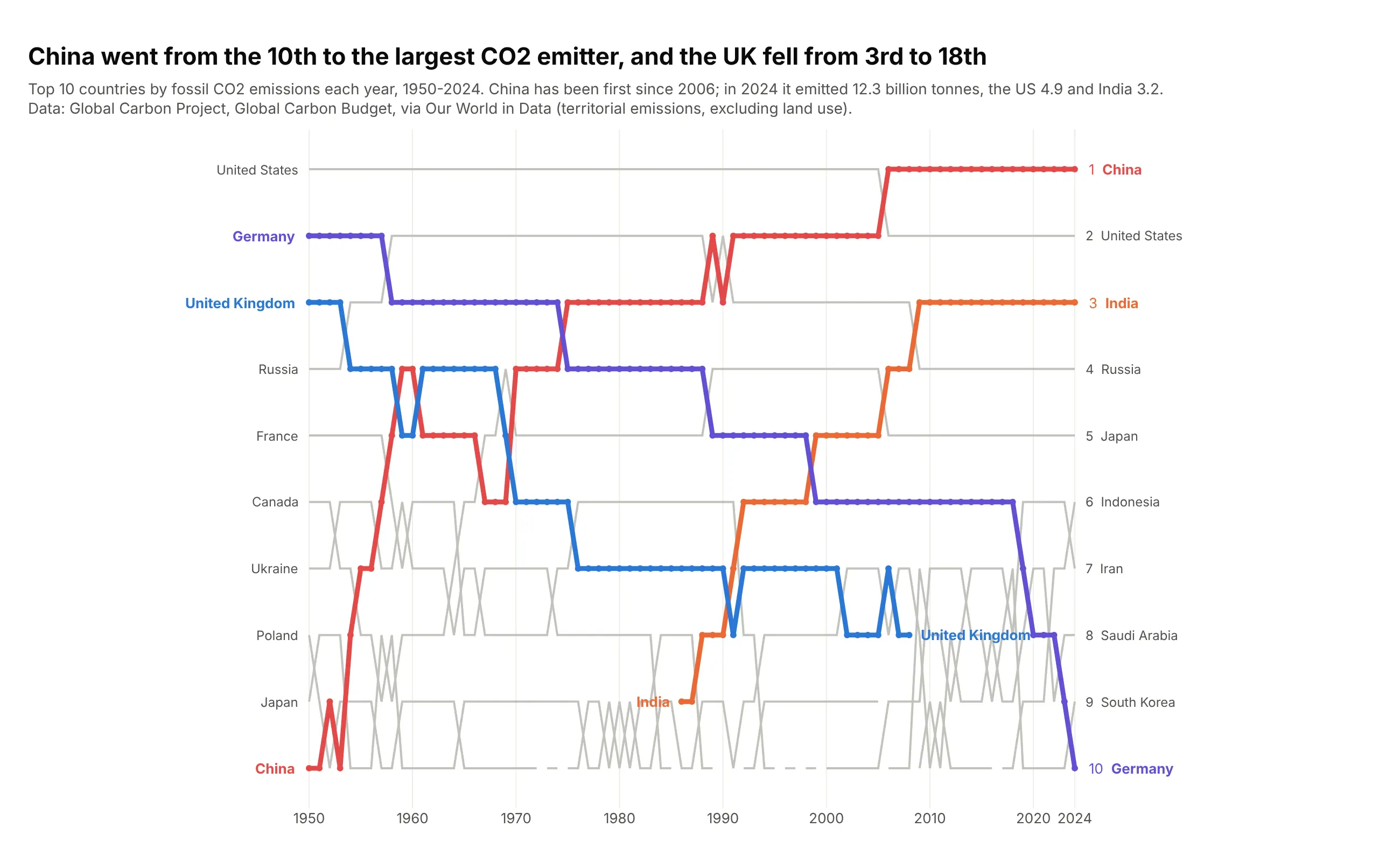
Bump chart of the 10 largest CO2 emitters from 1950 to 2024. China rises from 10th to 1st, India to 3rd; the UK falls out after 2008 and Germany falls to 10th

China went from the 10th largest emitter of fossil CO2 in 1950 to the largest in 2006, and emitted 12.3 billion tonnes in 2024. The UK, 3rd in 1950, left the top 10 after 2008 and is now 18th. Data: Global Carbon Project, via Our World in Data.

Tip: label the last point of a line that leaves the chart, so readers see it fell below the cut and didn't vanish from the data.

Get the data from Our World in Data's CO2 dataset (Global Carbon Project), fossil CO2 emissions
by country in million tonnes, 1950-2024, countries only
(columns: year, country, co2_mt, rank).

Build a plotly bump chart of the top 10 emitters.
- China and India in warm colors, the UK and Germany in cool colors; straight lines.
- Label the UK's line where it leaves the top 10.

6. Solar power leaders

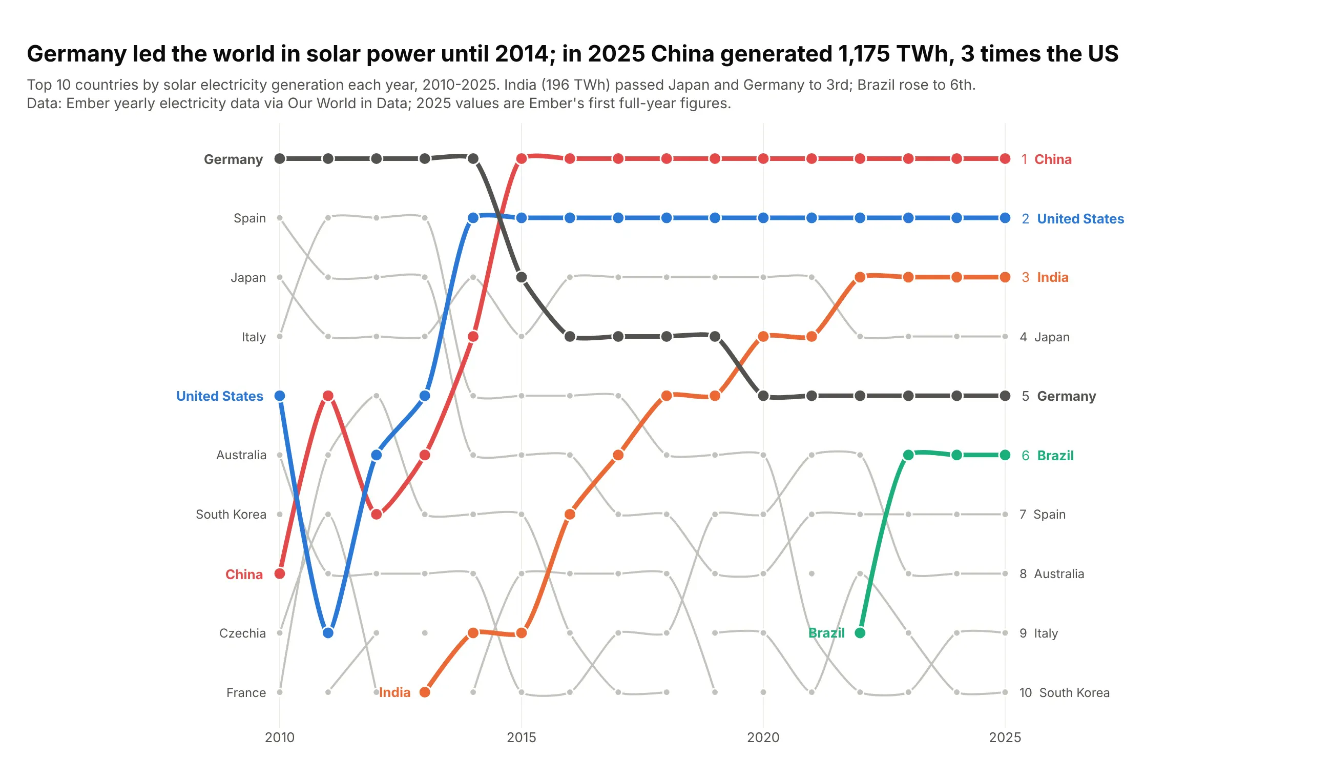
Bump chart of the 10 largest solar power generators from 2010 to 2025. Germany leads until 2014, China from 2015; India climbs from 15th to 3rd and Brazil enters at 9th in 2022

Germany generated the most solar power until 2014. By 2025 China generated 1,175 TWh, 3 times the US, and India had climbed from 15th in 2010 to 3rd. Data: Ember, via Our World in Data.

Tip: a fast-growing market is where ranks beat values, because 2010's leaders would be a flat line at zero next to 2025.

Get the data from Our World in Data's energy dataset (from Ember), solar electricity generation
in TWh by country, 2010-2025 (columns: year, country, twh, share_of_country_pct, rank).

Build a plotly bump chart of the top 10.
- China, the US, India, Germany and Brazil in color; spline lines.
- Title: when Germany lost first place and China's 2025 output vs the US.

7. The largest drugmakers by revenue

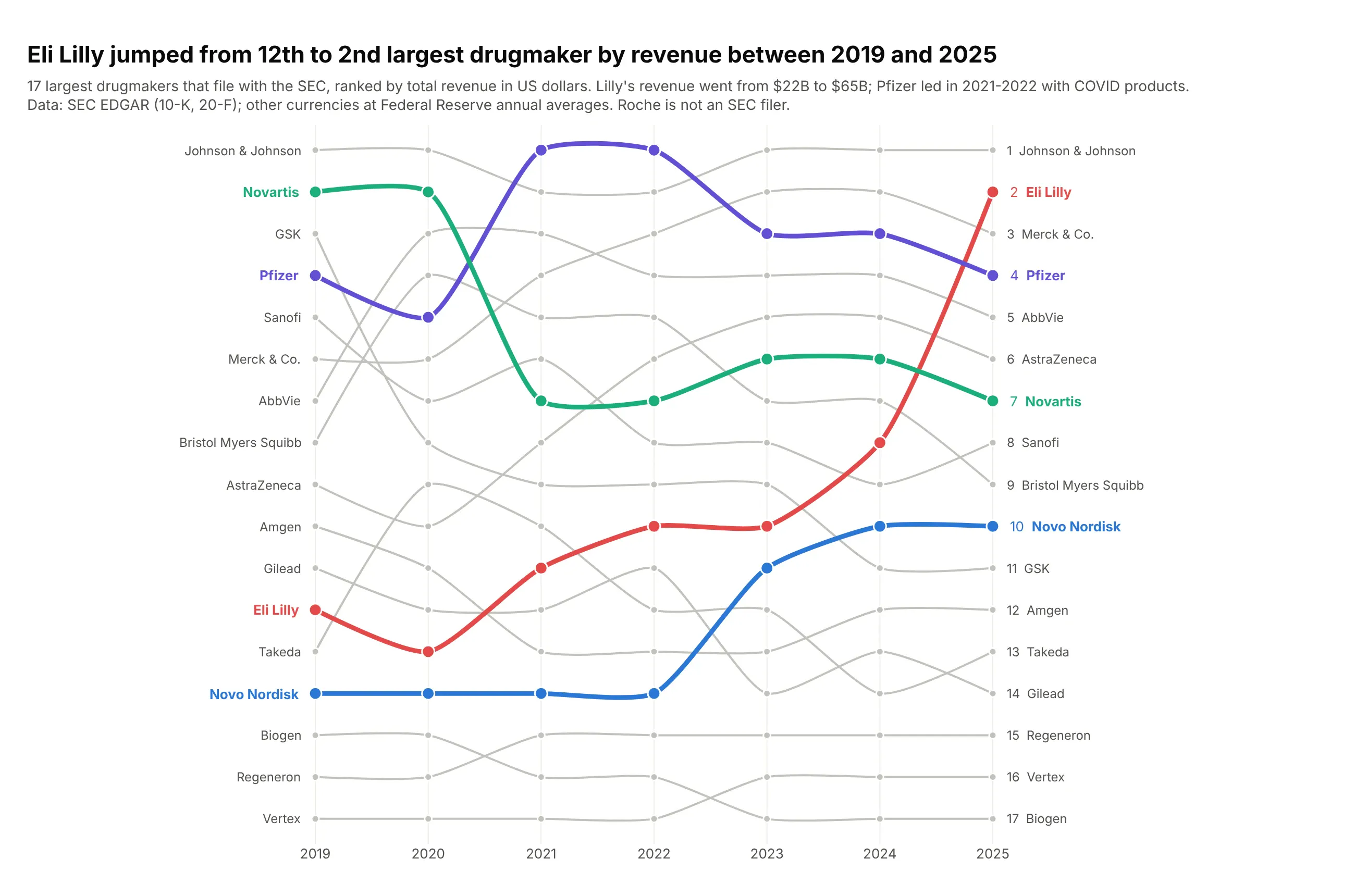
Bump chart of 17 drugmakers ranked by revenue in US dollars from 2019 to 2025. Eli Lilly climbs from 12th to 2nd, Novo Nordisk from 14th to 10th, Pfizer peaks at 1st in 2021-2022 and Novartis falls from 2nd to 7th

Eli Lilly jumped from 12th to the 2nd largest drugmaker by revenue between 2019 and 2025, as its revenue grew from $22B to $65B. Pfizer led in 2021 and 2022 with its COVID products. Data: SEC EDGAR (10-K and 20-F), Federal Reserve exchange rates.

Tip: when the list is short, show every company (top_n=17) so no line breaks.

Get the data from SEC EDGAR XBRL company facts (10-K and 20-F total revenue) for the 17 largest
drugmakers that file with the SEC, 2019-2025, converted to US dollars at Federal Reserve annual
average rates (columns: year, company, currency, revenue_local_bn, revenue_usd_bn, rank).

Build a plotly bump chart of all 17 companies.
- Eli Lilly, Novo Nordisk, Pfizer and Novartis in color; spline lines.
- Subtitle: Roche is not an SEC filer.

8. Who starts the most clinical trials

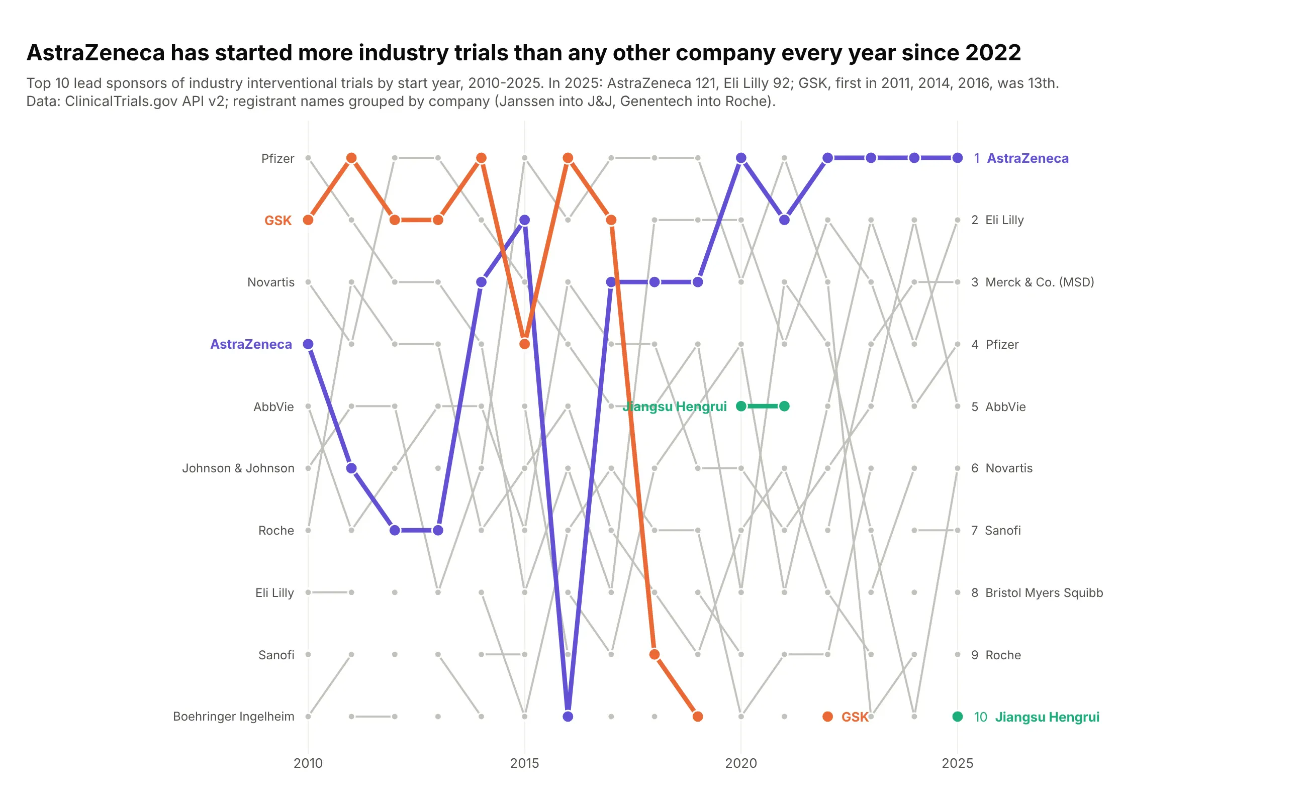
Bump chart of the 10 largest industry sponsors of new interventional trials on ClinicalTrials.gov by start year, 2010-2025. AstraZeneca has been first since 2022; GSK falls from first; Jiangsu Hengrui enters

AstraZeneca has started more industry-led interventional trials than any other company every year since 2022 (121 in 2025). GSK, first in 2011, 2014 and 2016, was 13th in 2025, and Jiangsu Hengrui was 10th. Data: ClinicalTrials.gov API v2.

Tip: normalize registrant names to companies before ranking (Janssen into J&J, Genentech into Roche), or one company splits into several lines.

Get the data from the ClinicalTrials.gov API v2: every industry-led interventional study with a
start date in 2010-2025 (fields: NCTId, LeadSponsorName, StartDate), lead sponsors normalized to
companies, counted by start year (columns: year, sponsor, trials, rank).

Build a plotly bump chart of the top 10 sponsors per year.
- AstraZeneca, GSK and Jiangsu Hengrui in color; straight lines.
- Print sponsors whose rank changes by more than 5 places in one year.

9. Leading causes of death in the US

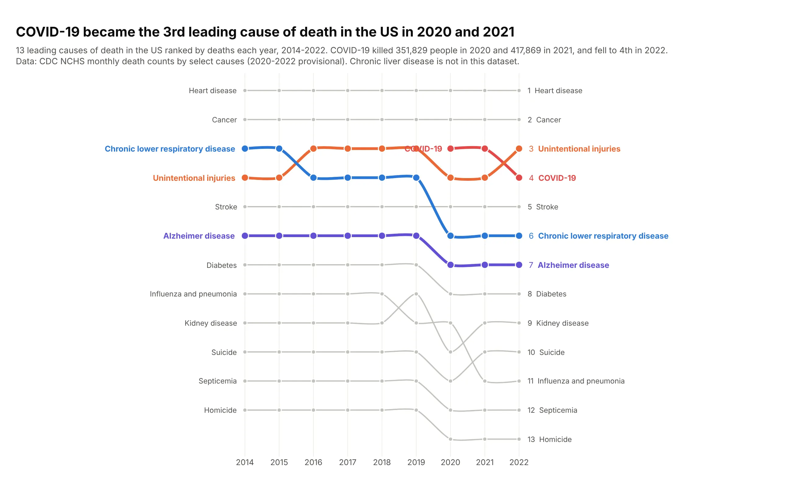
Bump chart of 13 causes of death in the US ranked by deaths from 2014 to 2022. COVID-19 enters at 3rd in 2020 and 2021 and falls to 4th; chronic lower respiratory disease and Alzheimer disease move down

COVID-19 became the 3rd leading cause of death in the US in 2020 (351,829 deaths) and 2021 (417,869), and fell to 4th in 2022. Every cause below it moved down one place. Data: CDC NCHS monthly death counts (2020-2022 provisional).

Tip: a new entry pushes everything below it down, so highlight one or two of the displaced lines to show that.

Get the data from CDC NCHS on data.cdc.gov: "Monthly Counts of Deaths by Select Causes,
2014-2019" and "Monthly Provisional Counts of Deaths by Select Causes, 2020-2023", United States,
summed by year for 13 rankable causes, 2014-2022 (columns: year, cause, deaths, rank).

Build a plotly bump chart of all 13 causes.
- COVID-19 in red; unintentional injuries, chronic lower respiratory disease and Alzheimer disease
  in color; spline lines.

10. Web browsers

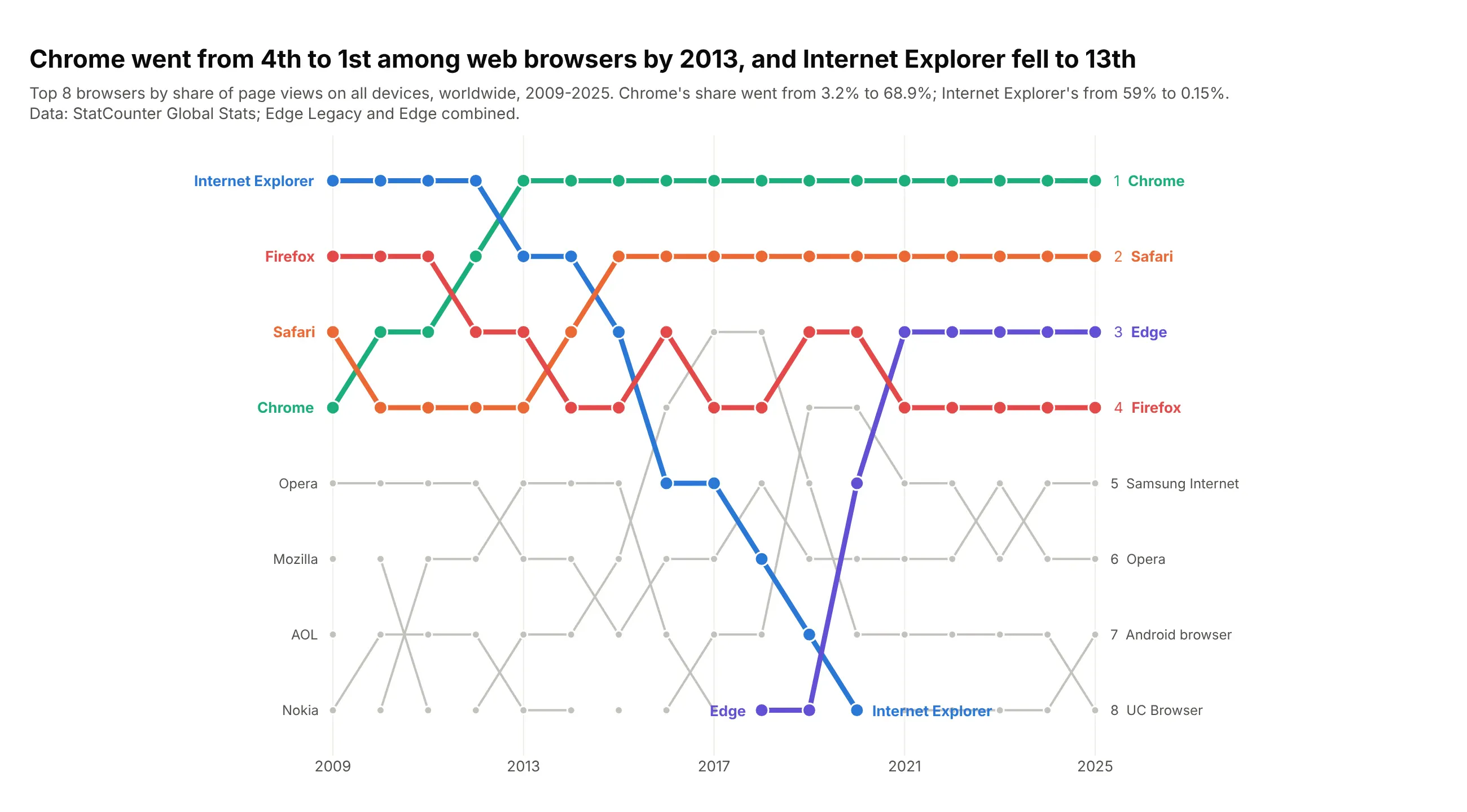
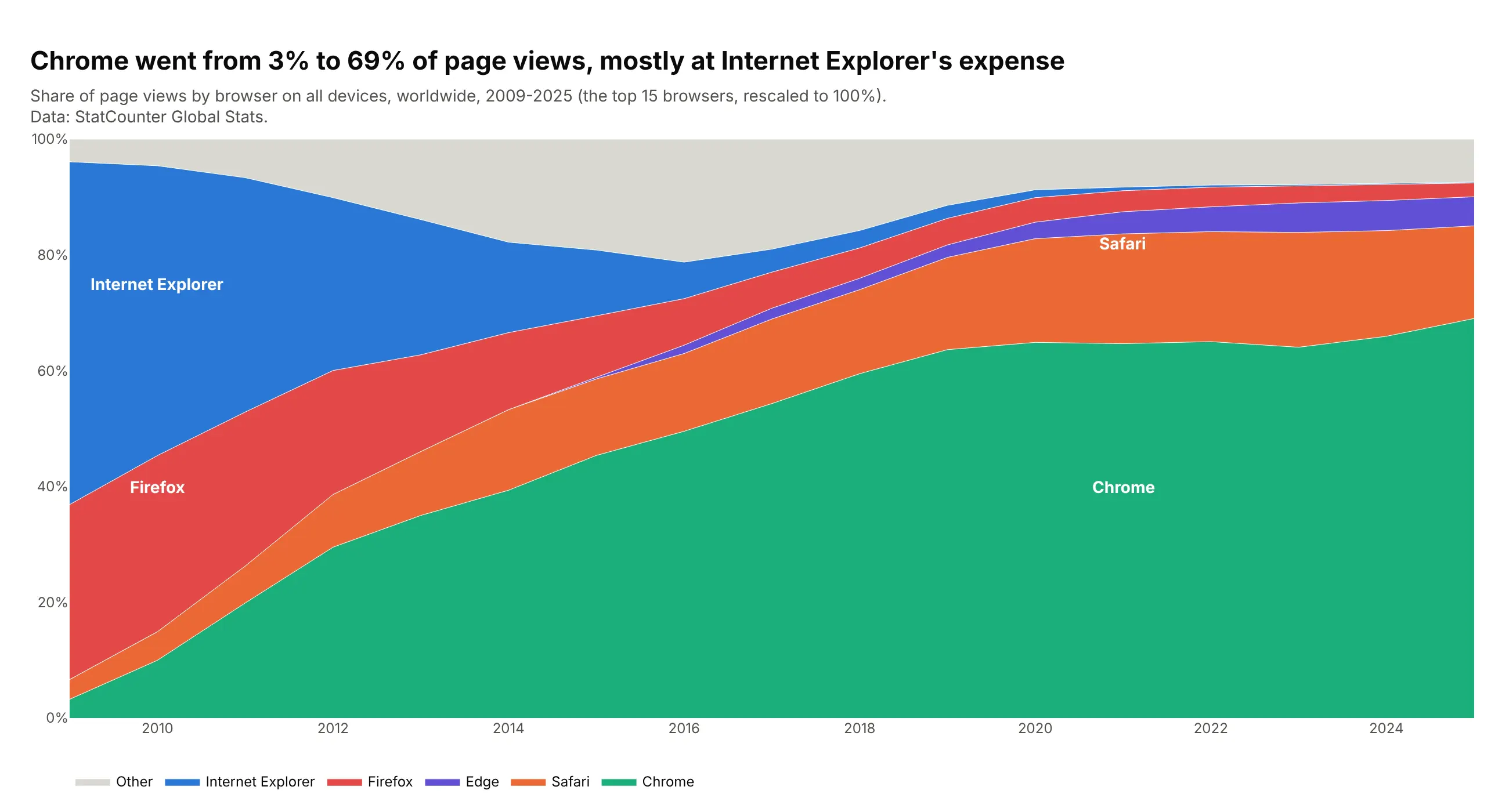
Bump chart of the top 8 browsers by share of page views from 2009 to 2025. Chrome rises from 4th to 1st by 2013; Internet Explorer falls out after 2020; Safari is 2nd; Edge enters and reaches 3rd

Chrome went from the 4th most used web browser in 2009 to 1st by 2013, and had 69% of page views in 2025. Internet Explorer, first in 2009 with 59%, was 13th in 2025. Data: StatCounter Global Stats.

Tip: join renamed products into one line (Edge Legacy and Edge) before you rank.

Get the data from StatCounter Global Stats, browser market share on all platforms, worldwide,
yearly 2009-2025 (columns: year, browser, share_pct, rank), with Edge Legacy and Edge combined.

Build a plotly bump chart of the top 8 browsers.
- Chrome, Internet Explorer, Safari, Edge and Firefox in color; straight lines.
- Label where Internet Explorer leaves and Edge enters.

Another way to see it: shares add up to 100%, so a stacked area shows where Chrome's share came from.