
Chris Parmer
November 3, 2026
Density Plots - A Complete Guide
TL;DR
- A density plot draws the distribution of one numeric variable as a smooth curve, a kernel density estimate (KDE), whose height shows where values are common and whose area under the curve is 1. A 2D density plot does the same for two variables, as a heatmap of counts or as contours.
- Density plots are also known as KDE plots, kernel density plots and density trace graphs, their 2D versions as 2D histograms and density heatmaps, and they are similar to histograms, violin plots and ridgeline plots.
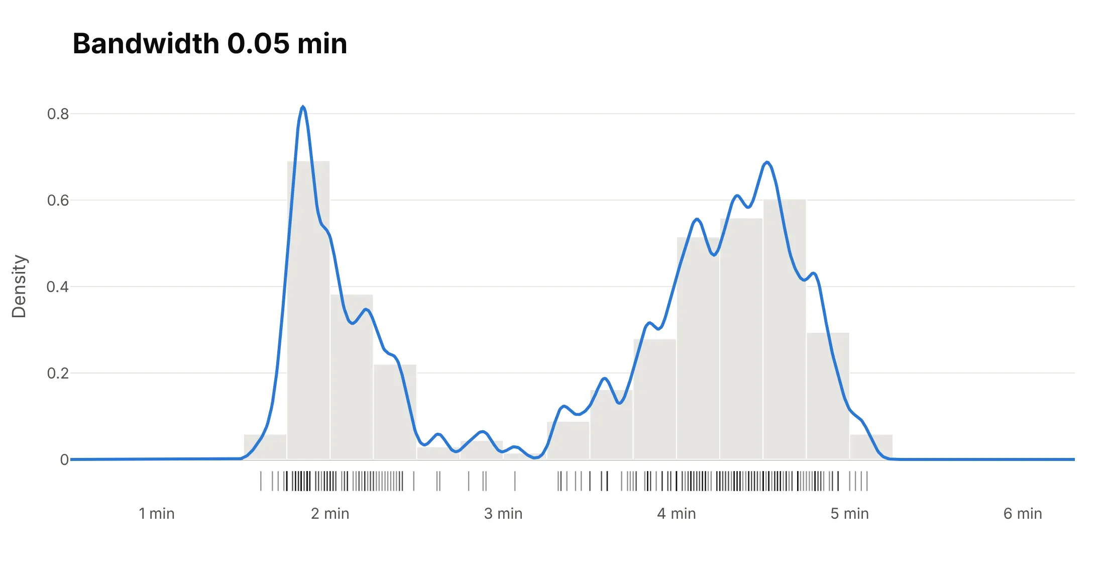
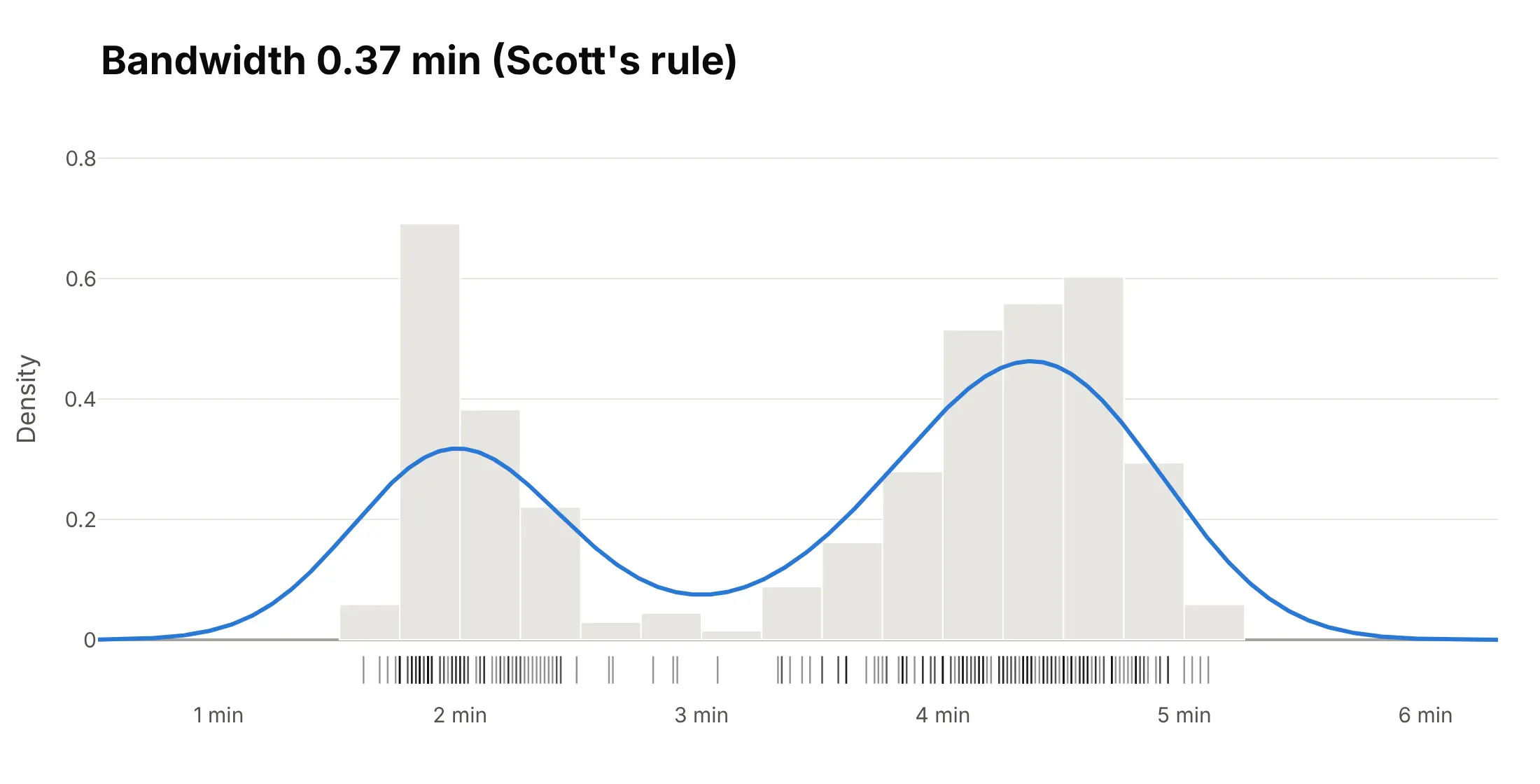
- The one setting that changes what a density plot says is the bandwidth. On Old Faithful's eruptions, 0.05 minutes gives 12 bumps, Scott's rule (0.37 minutes) gives the two real groups, and 1 minute merges them into one hump.
- In Python, compute the curve with scipy.stats.gaussian_kde and draw it with go.Scatter; for two variables, Plotly Express has px.density_heatmap and px.density_contour. This is how you make the equivalent of seaborn's kdeplot, displot and histplot(kde=True) with Plotly.
What is a density plot?
Density plots look like this:
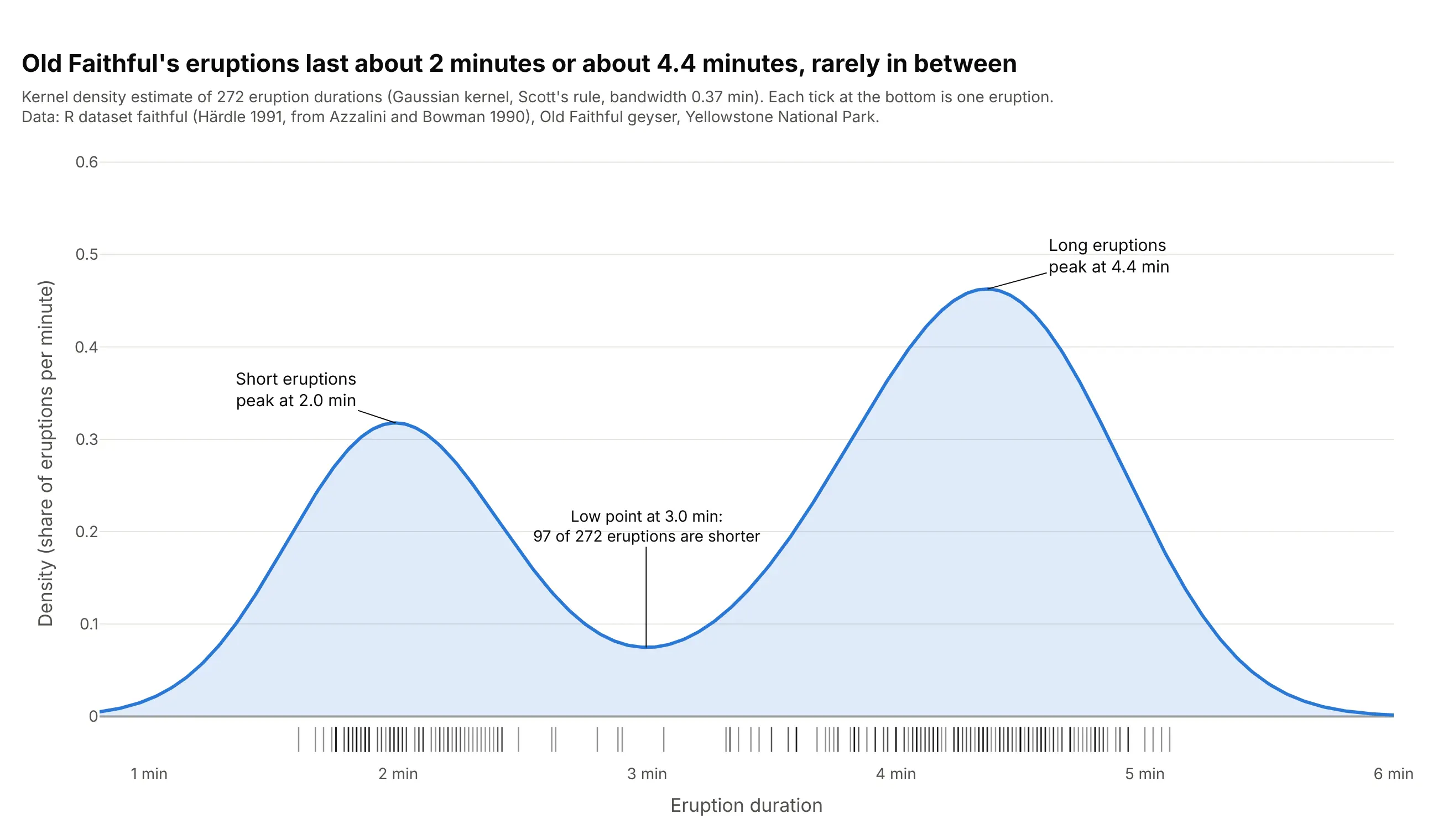
Data: R dataset faithful, the Old Faithful geyser in Yellowstone National Park (Azzalini and Bowman 1990, via Härdle 1991).
How do you read a density plot? In the example above, notice these things:
- The curve is high where many eruptions have similar durations. It peaks at 2.0 minutes and at 4.4 minutes, so Old Faithful has short eruptions and long ones.
- The low point at 3.0 minutes is the gap between the two groups: 97 of the 272 eruptions are shorter than that and 175 are longer.
- The height is a density, a share of eruptions per minute, so the total area under the curve is 1 (100% of the eruptions). The area between two durations is the share of eruptions in that range.
- Each tick along the bottom is one eruption. The curve is the sum of a small bell curve centered on every tick, each 0.37 minutes wide (the bandwidth, set here by Scott's rule).
It's often used for charts like these:
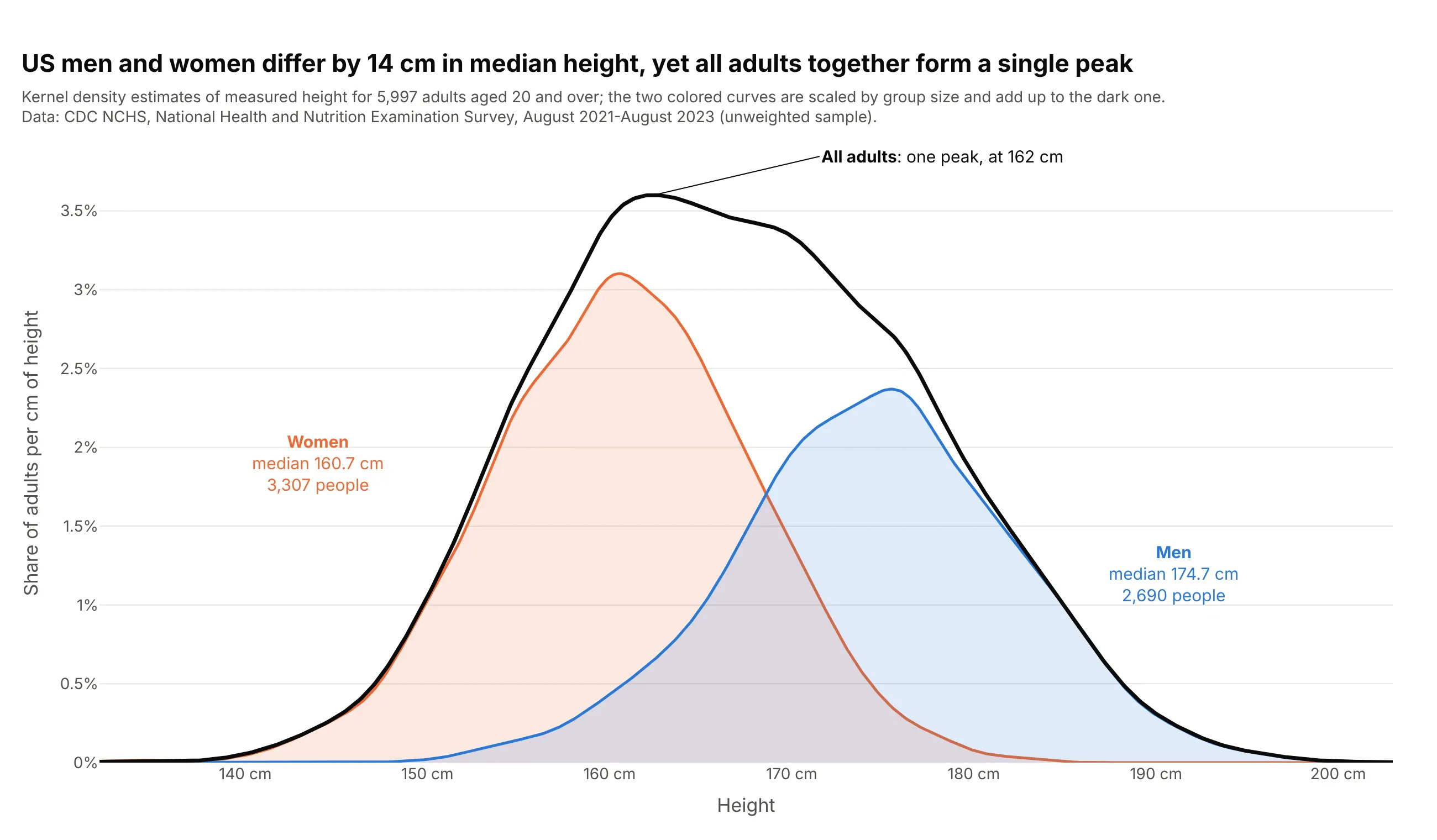
Human heights. US men's median height is 14 cm above women's, yet all adults together form a single peak at 162 cm, because two groups only make two peaks when they're far apart compared with their spread (Schilling, Watkins and Watkins 2002). Data: CDC NCHS, NHANES August 2021-August 2023.

Fat tails in financial returns. On a log scale, the density of daily US stock returns falls far more slowly than a normal curve: 101 days since 1926 moved more than 5 standard deviations, where a normal distribution expects 0.015. Data: Kenneth R. French Data Library, from CRSP; the classic study is Mandelbrot (1963).
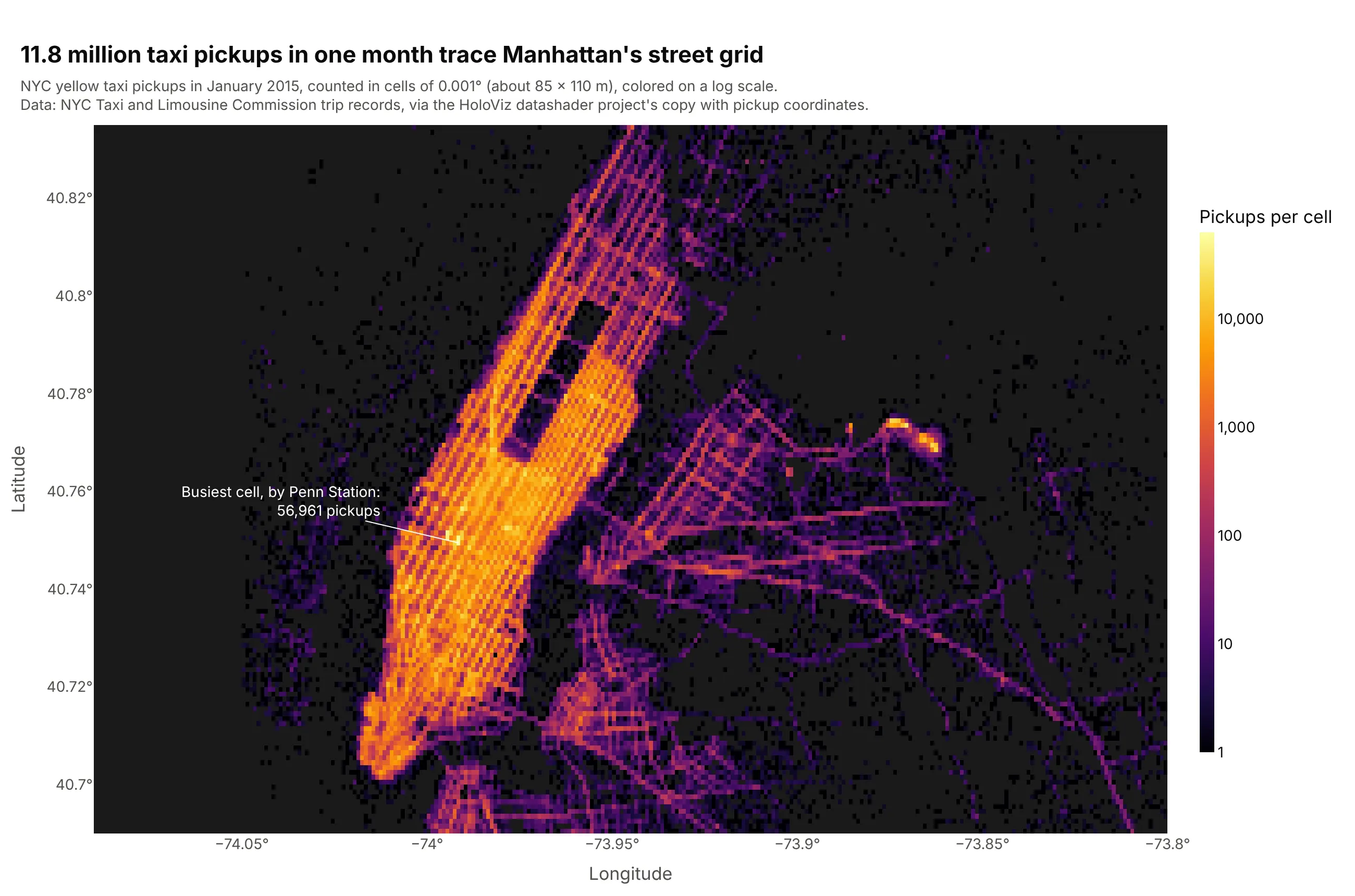
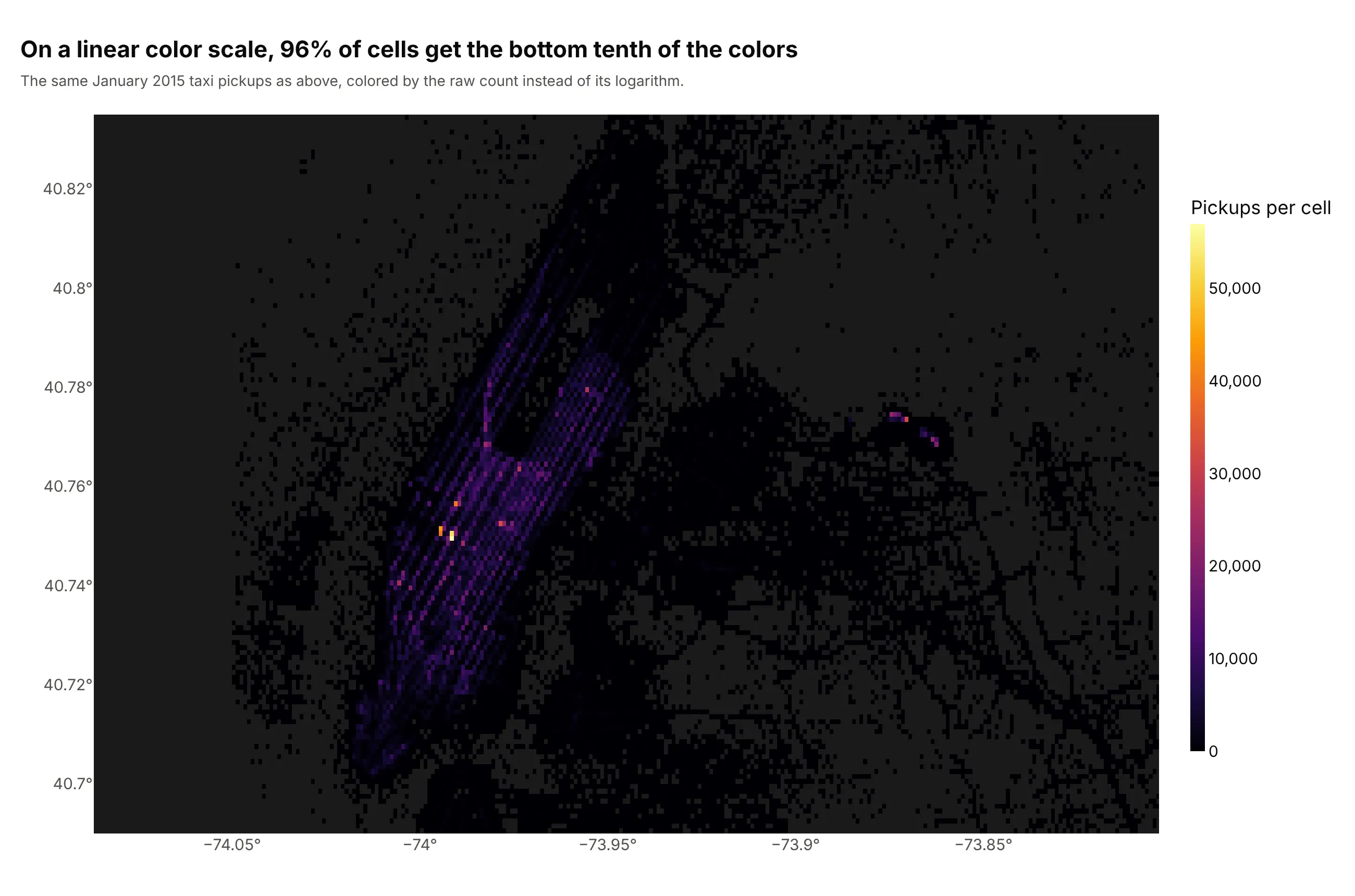
2D density of a large point cloud. Drawn as dots, 11.8 million taxi pickups overlap into one blob; counted in 0.001-degree cells and colored on a log scale, they show Manhattan's avenues and a busiest cell of 56,961 pickups by Penn Station. Data: NYC Taxi and Limousine Commission, January 2015, via the coordinate copy used in datashader's NYC taxi example.
A short history
Kernel density estimation was introduced by Rosenblatt (1956) and Parzen (1962), which is why it's also called the Parzen-Rosenblatt window method. Bernard Silverman's 1986 book Density Estimation for Statistics and Data Analysis used 107 Old Faithful eruption lengths from Weisberg (1980) as an example dataset, which is one reason the geyser became the textbook case for density plots. This is a kernel density estimate of those same 107 eruptions, redrawn with Plotly using his rule-of-thumb bandwidth:
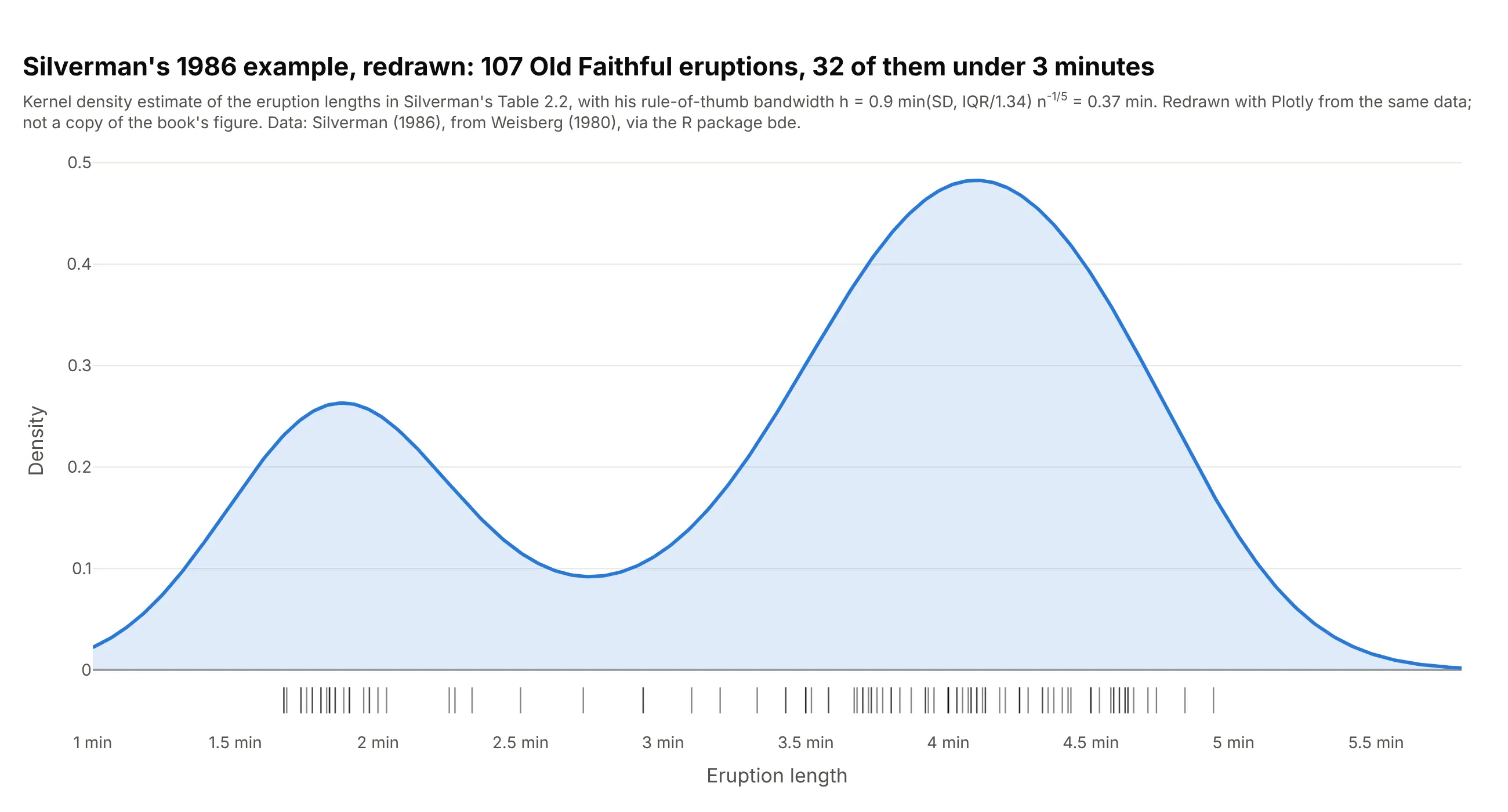
Data: Silverman (1986), Table 2.2, from Weisberg (1980), via the R package bde. A redraw from the same data, not a copy of the book's figure.
How to choose the bandwidth
A kernel density estimate puts a small bell curve (the kernel) on every value and adds them up. The bandwidth is the width of those bell curves, and it decides what the plot shows: too narrow and every cluster of a few values becomes its own peak, too wide and real groups melt together. Here are Old Faithful's 272 eruptions three ways, over a light histogram for reference.
Too narrow. With a bandwidth of 0.05 minutes, the curve has 12 peaks. Most of them are a handful of eruptions that happen to sit close together, and they would move if you measured another 272 eruptions.
Scott's rule. The default in scipy's gaussian_kde and seaborn's kdeplot picks 0.37 minutes here (the standard deviation times n to the power -1/5). The two groups are clear and the noise is gone. scipy's "silverman" option gives a similar 0.39 minutes.
Too wide. With a bandwidth of 1 minute, the two groups merge into one hump at 4.1 minutes, and the curve suggests eruptions of 1 or 6 minutes, which never happened in this data.
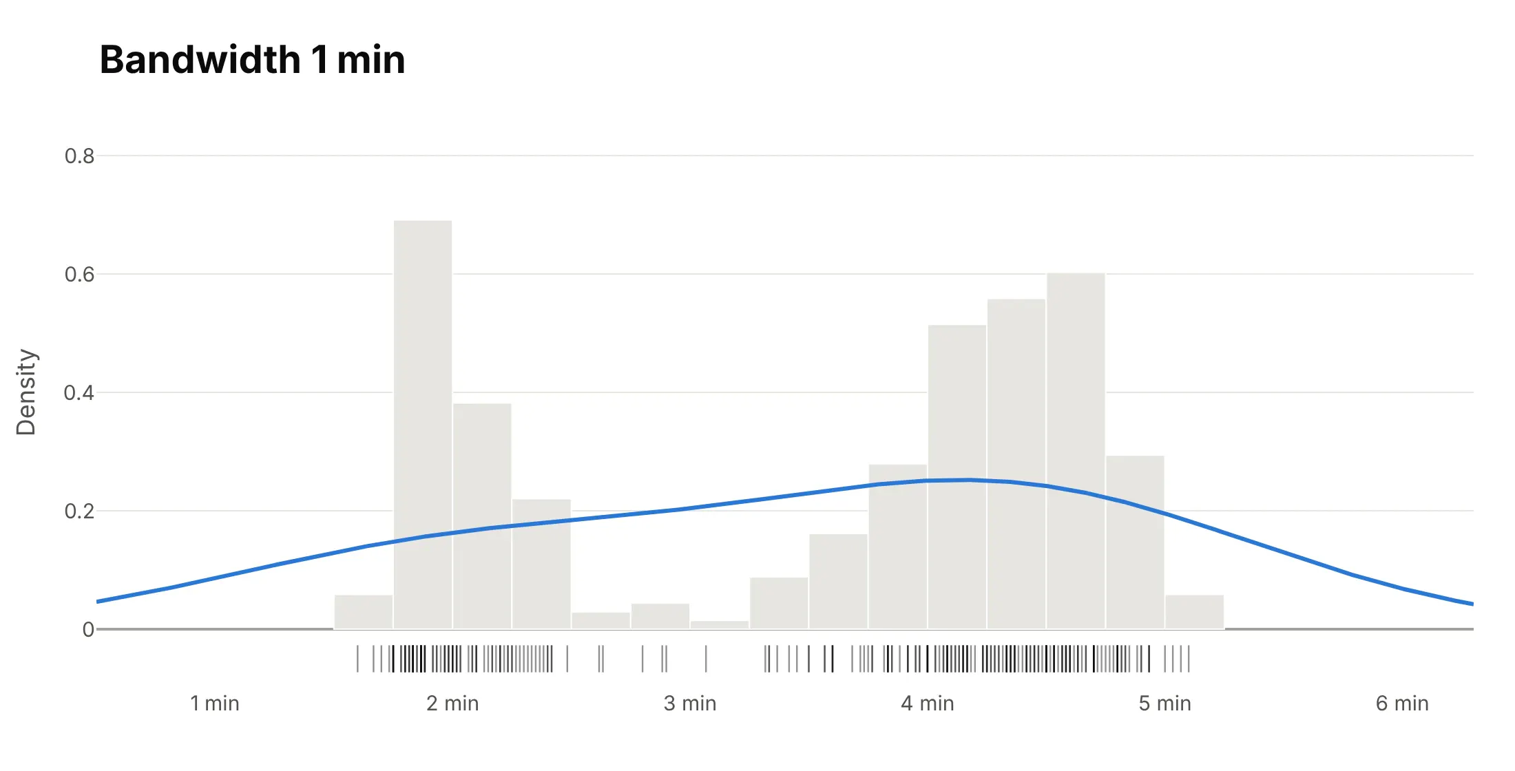
The rules of thumb assume the data is roughly bell-shaped. The scipy documentation warns that "bimodal or multi-modal distributions tend to be oversmoothed", so with two or more groups, try a bandwidth a half or a third of the default and see whether a peak appears that the data supports. Always show the bandwidth in the subtitle, and add a rug or a histogram underneath when the reader needs to check the curve against the data.
Alternatives to a density plot
Here are Old Faithful's 272 eruption durations drawn six ways. Some are better for the question, some worse, some just different:
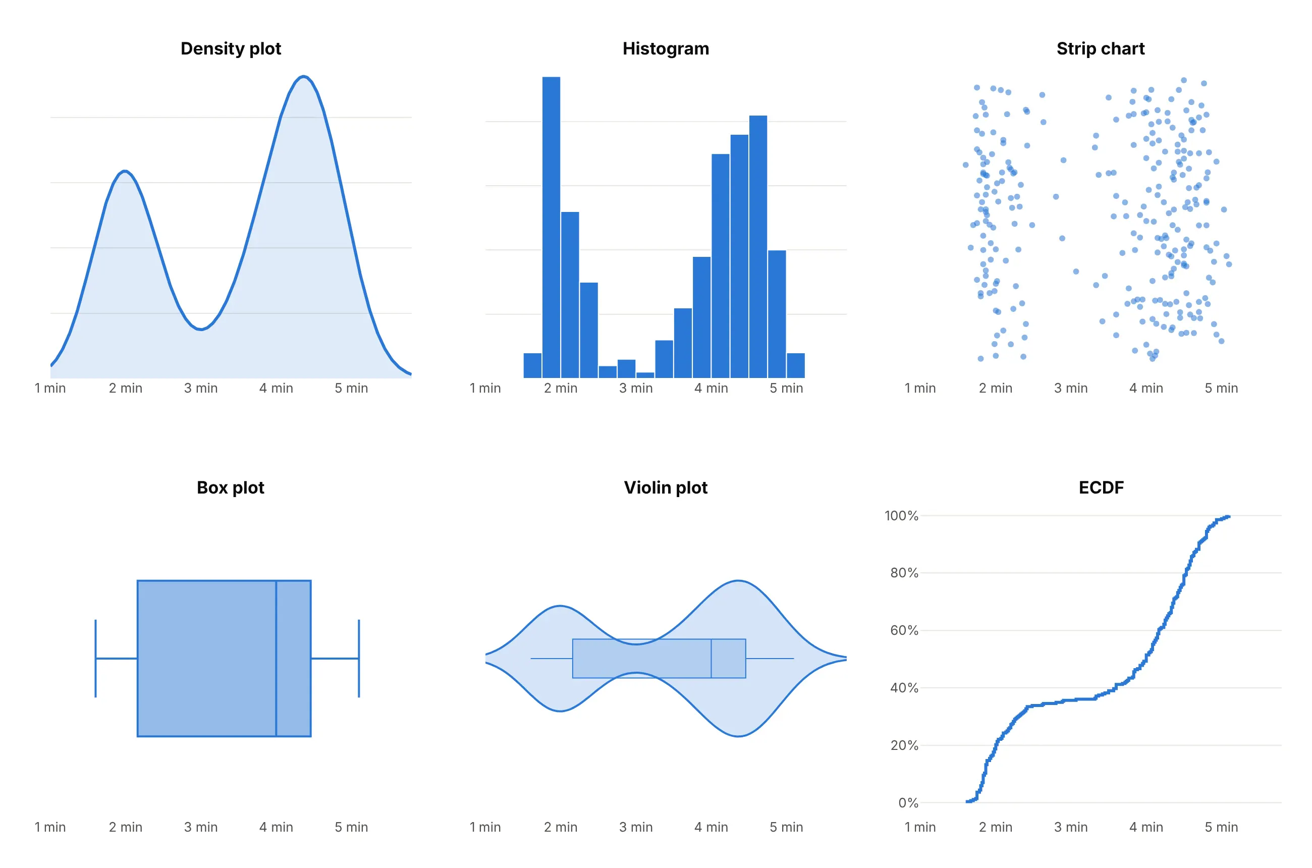
- Histogram (works too, and better for exact counts). The bars show how many eruptions fall in each 15-second bin, and nothing is smoothed, but the shape depends on where the bins start and how wide they are.
- Strip chart (better for small data). Every eruption is a dot, so nothing is hidden, though past a few thousand points the dots merge.
- Box plot (worse here). The box runs from 2.2 to 4.5 minutes, right across the gap, so it hides that there are two groups.
- Violin plot (different, better for comparing groups). A violin is a density plot mirrored around a center line, which makes it easy to put many groups side by side.
- ECDF (better for "what share is below X"). The flat stretch near 3 minutes is the gap, and you can read exact percentiles off it, but the two peaks are harder to see.
- Ridgeline plot (better for many groups). A ridgeline stacks one density plot per group in rows, as in the trial example below.
For two variables, here are the same eruptions with the wait until the next eruption, drawn four ways:
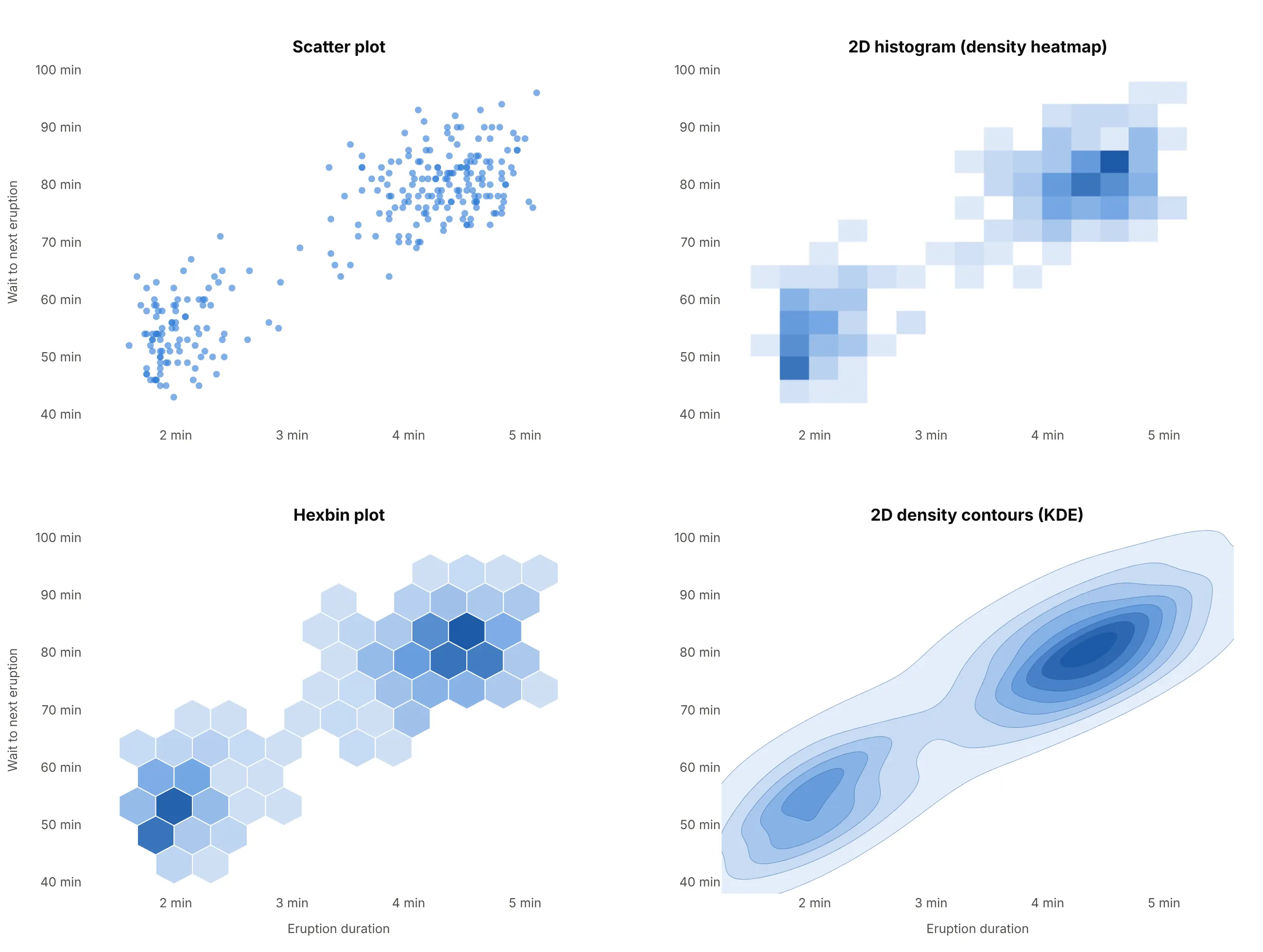
- Scatter plot (better for a few hundred points). Every eruption is visible, and with 272 points nothing overlaps much.
- 2D histogram or density heatmap (better for large data). px.density_heatmap counts points in rectangular cells, which stays fast and exact with millions of points.
- Hexbin plot (works too). The same counting with hexagons, which look less blocky.
- 2D KDE contours (better for smooth shapes in small data). A 2D kernel density estimate drawn as filled contours, the equivalent of seaborn's kdeplot(x=..., y=...); see the contour plot guide for more ways to style contours.
How to make a density plot
With AI
ChatGPT, Claude Code, GitHub Copilot, Cursor and other AI tools are excellent at writing Plotly code. Name Plotly in the prompt, and say how the bandwidth should be chosen and what goes under the curve:
Make a plotly density plot from faithful.csv (columns: eruptions, waiting).- Compute a Gaussian kernel density estimate of eruptions with scipy.stats.gaussian_kde (Scott's rule)and draw it with go.Scatter and a light fill.- Add a rug: one tick per eruption along the bottom.- Label both peaks and the low point between them with their durations.- Put the bandwidth in minutes in the subtitle, and use a title that states the takeaway.- Check: print the bandwidth and the durations of the peaks.
With Plotly Studio
Plotly Studio is a desktop app where you point an AI at a dataset and it builds charts and a Dash app around your questions. Ask for a density plot the same way:
Show a density plot of total cholesterol for 1999-2000 and 2021-2023 on one axis, weighted by the survey weights, with a line at 240 mg/dL and the share of adults above it for each survey.
Make a density plot in Python or JavaScript
This is the code AI tools write under the hood. In Python, scipy.stats.gaussian_kde computes the curve and go.Scatter draws it, with a rug of the raw values underneath:
import numpy as npimport pandas as pdimport plotly.graph_objects as gofrom scipy.stats import gaussian_kdeurl = "https://raw.githubusercontent.com/vincentarelbundock/Rdatasets/master/csv/datasets/faithful.csv"x = pd.read_csv(url).eruptions # 272 eruption durations, in minuteskde = gaussian_kde(x) # Scott's rule; bw_method="silverman" or a number to change itgrid = np.linspace(1, 6, 500)fig = go.Figure(go.Scatter(x=grid, y=kde(grid), mode="lines", fill="tozeroy", name="Density"))fig.add_trace(go.Scatter(x=x, y=np.zeros(len(x)), mode="markers", name="Eruptions", # a rug of the raw valuesmarker=dict(symbol="line-ns-open", size=12, color="black")))fig.update_layout(xaxis_title="Eruption duration (min)", yaxis_title="Density", showlegend=False)fig.show()
gaussian_kde takes weights= for survey or frequency weights (example 5 below uses it) and a 2D array for a 2D estimate (example 1). In plotly.py 7, this replaces figure_factory.create_distplot, which was removed in version 7.0 after being deprecated. To put a density curve over a histogram, as seaborn's histplot(kde=True) does, add a go.Histogram with histnorm="probability density" so the bars and the curve share one scale (example 6).
For two variables, Plotly Express makes a 2D density plot in one line of code. px.density_heatmap counts the points in a grid of cells (a 2D histogram) and px.density_contour draws contours of the same counts; the 2D histogram docs and the density contour docs cover the options:
import pandas as pdimport plotly.express as pxurl = "https://raw.githubusercontent.com/vincentarelbundock/Rdatasets/master/csv/datasets/faithful.csv"df = pd.read_csv(url)fig = px.density_heatmap(df, x="eruptions", y="waiting", nbinsx=20, nbinsy=20, marginal_x="histogram")fig.show()fig = px.density_contour(df, x="eruptions", y="waiting")fig.update_traces(contours_coloring="fill", colorscale="Blues")fig.show()
Both are fast with millions of points because the browser bins them. For smooth 2D KDE contours like example 1, evaluate a 2D gaussian_kde on a grid and draw it with go.Contour.
In JavaScript, plotly.js draws the same curve from a scatter trace; the kernel density estimate is a few lines of code:
<div id="chart"></div><script src="https://cdn.plot.ly/plotly-4.1.1.min.js"></script><script>// Old Faithful eruption durations (R dataset faithful), drawn as a Gaussian KDE with Scott's rulefetch("https://raw.githubusercontent.com/vincentarelbundock/Rdatasets/master/csv/datasets/faithful.csv").then(r => r.text()).then(text => {const x = text.trim().split("\n").slice(1).map(line => +line.split(",")[1]);const n = x.length, mean = x.reduce((a, b) => a + b) / n;const sd = Math.sqrt(x.reduce((a, b) => a + (b - mean) ** 2, 0) / (n - 1));const h = sd * n ** -0.2; // Scott's rule, as in scipyconst grid = Array.from({length: 400}, (_, i) => 1 + i * 5 / 399);const density = grid.map(g => x.reduce((s, xi) => s + Math.exp(-0.5 * ((g - xi) / h) ** 2), 0)/ (n * h * Math.sqrt(2 * Math.PI)));Plotly.newPlot("chart", [{type: "scatter", x: grid, y: density, mode: "lines", fill: "tozeroy", line: {color: "#2a78d6", width: 3}},{type: "scatter", x: x, y: x.map(() => 0), mode: "markers", // rugmarker: {symbol: "line-ns-open", size: 12, color: "black"}}], {width: 800, height: 400, showlegend: false,xaxis: {title: {text: "Eruption duration (min)"}}, yaxis: {title: {text: "Density"}}});});</script>
plotly.js also computes kernel density estimates itself inside violin traces: a violin trace with side: "positive" draws one half of the violin, which is a density plot with its bandwidth set by Silverman's rule unless you pass bandwidth.
Share it
Every Plotly chart has a Share chart button (the cloud icon in its toolbar) that uploads it to Plotly Cloud and gives you a link. Only you can see it until you change its visibility.
For a live app, put the chart in a Dash app and publish it with the Plotly Cloud CLI. Coding agents can run these commands for you:
pip install "dash[cloud]"plotly user loginplotly app publish
If your data has to stay in your own cloud or data center, publish to Dash Enterprise instead.
Dos and don'ts
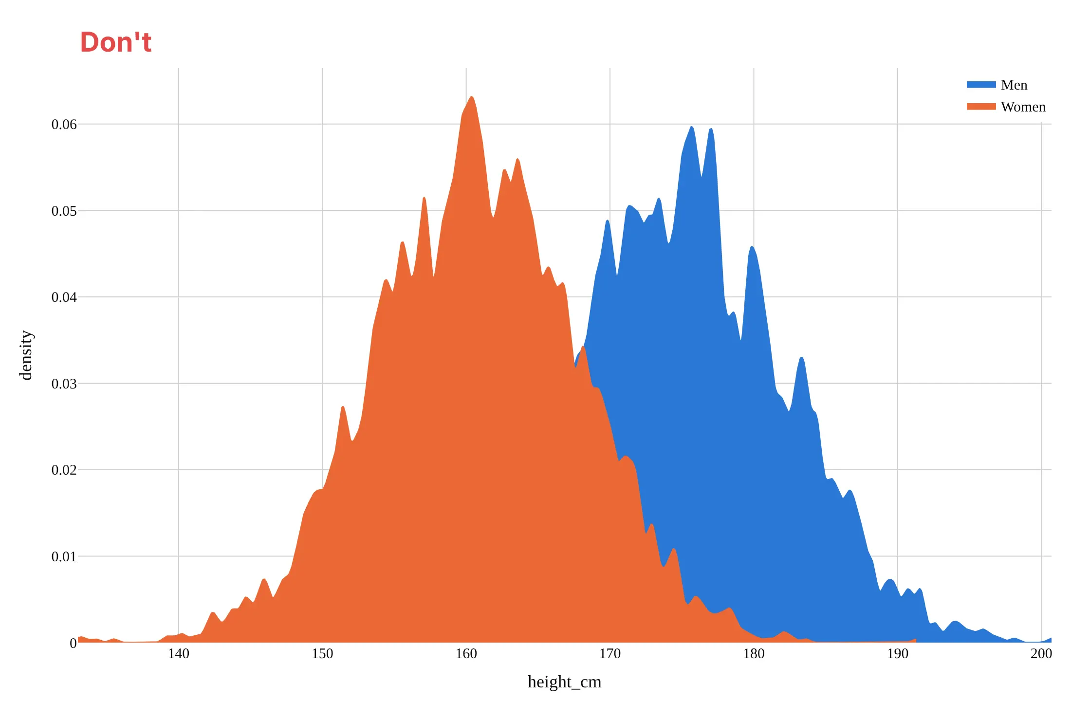
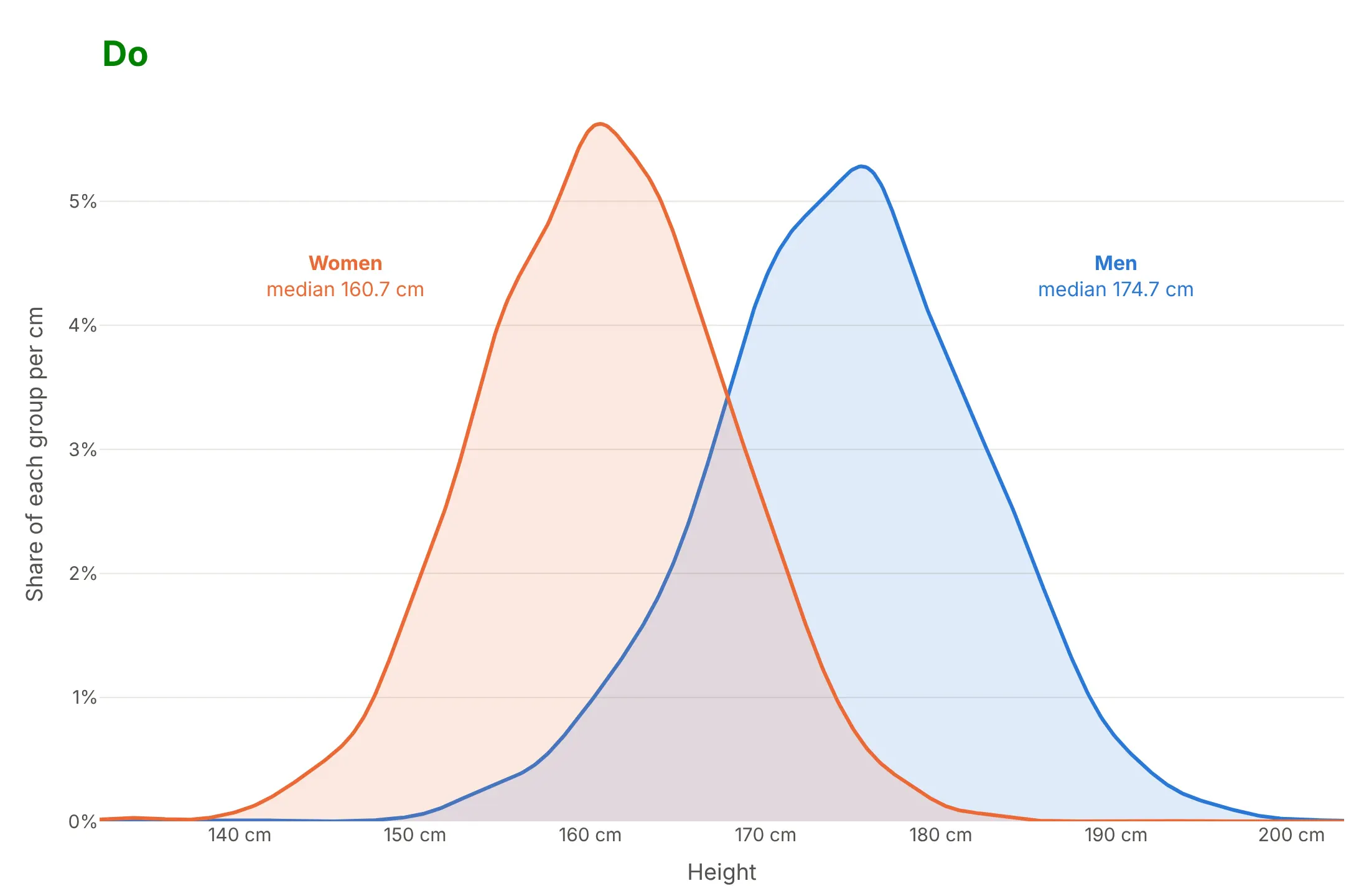
Most of the work in a published density plot is choosing the bandwidth, letting the curves finish and making overlapping groups readable. Here are the heights of 5,997 US adults both ways, in the same colors.
Don't use a bandwidth so small that measurement noise turns into peaks, stop each curve at its group's smallest and largest value, fill the curves with opaque color so one group hides the other, or leave raw column names, a far-away legend and a default serif font:
Do use Scott's rule (or check a smaller bandwidth against the data), let the curves fade to zero past the data, use strong lines with light fills so the overlap shows, label the groups next to their curves and write the y axis in plain units:
Watch the boundaries
A Gaussian kernel doesn't know that a distance, a price or a count can't go below zero, so the curve leaks past the boundary. In example 6, 2.9% of the area of the NBA shot-distance curve falls below 0 feet. Three ways to handle it: compute the estimate on the logarithm of the values when they span orders of magnitude (example 4), cut the curve at the boundary and say so, or show a histogram next to the curve so the reader sees the real counts.
Use a log color scale for big point clouds
The 2D density plot of NYC taxi pickups above colors each cell by the logarithm of its count. On a linear scale, 96% of the cells fall in the bottom tenth of the colors, and only a few blocks of Midtown show:
Checklist
Do
- Put the bandwidth in the subtitle, and check a smaller one when you expect more than one group.
- Add a rug or a histogram when the data has fewer than a few hundred values, so readers can check the curve.
- Use light fills and strong lines when two or three curves overlap; use a ridgeline or small multiples for more.
- Scale each group's curve by its share when the groups should add up to a total, as in the heights chart above.
- Use a log axis, and compute the estimate on log values, for data that spans orders of magnitude.
- Write the y axis as a share per unit ("% of adults per cm") instead of "density".
Don't
- Use a density plot for a handful of values or for data with only a few distinct values; use a strip chart or a bar chart.
- Read peaks in the tails as real when only one or two values make them.
- Forget that px.density_heatmap and px.density_contour count points in bins, so their bin size plays the role of the bandwidth.
Options to customize
A density plot in Plotly is a go.Scatter line of a kernel density estimate, or one of the 2D traces Plotly Express makes, so these are the options that matter most. The full lists are in the scatter trace reference, the histogram2d reference and the scipy gaussian_kde documentation.
- gaussian_kde(x, bw_method=...): the bandwidth: "scott" (default), "silverman", or a number that multiplies the standard deviation; seaborn's bw_adjust=2 is bw_method=gaussian_kde(x).factor * 2.
- gaussian_kde(x, weights=...): survey or frequency weights, as in example 5.
- The evaluation grid: np.linspace a few bandwidths past the data so the curve fades to zero, or stop it at a hard boundary.
- fill="tozeroy", fillcolor: a light fill under each curve; use rgba colors at 0.15 opacity when curves overlap.
- marker.symbol="line-ns-open": rug ticks along the bottom, one per value.
- go.Histogram(histnorm="probability density"): a histogram on the same scale as the curve, as in seaborn's histplot(kde=True).
- xaxis.type="log": a log axis; compute the estimate on np.log10 of the values and plot against 10 ** grid.
- px.density_heatmap(x=..., y=..., nbinsx=..., nbinsy=...): a 2D histogram; add z= and histfunc="sum" for data that is already counted.
- marginal_x, marginal_y: histograms, box plots, violins or rugs on the margins of a px.density_heatmap or px.density_contour.
- px.density_contour, contours_coloring="fill": filled contour bands of the binned counts.
- go.Contour(z=...) with a 2D gaussian_kde evaluated on a grid: smooth 2D KDE contours.
- go.Violin(side="positive"): a half violin, which is a density plot computed in the browser; bandwidth sets its width.
- color_continuous_scale, range_color: the color scale of a density heatmap; cap it when a few cells would use up the whole scale.
More density plot examples
Seven more density plots built from real public data, each with its source, the technique that makes it work and a prompt to rebuild it.
1. Old Faithful in two dimensions
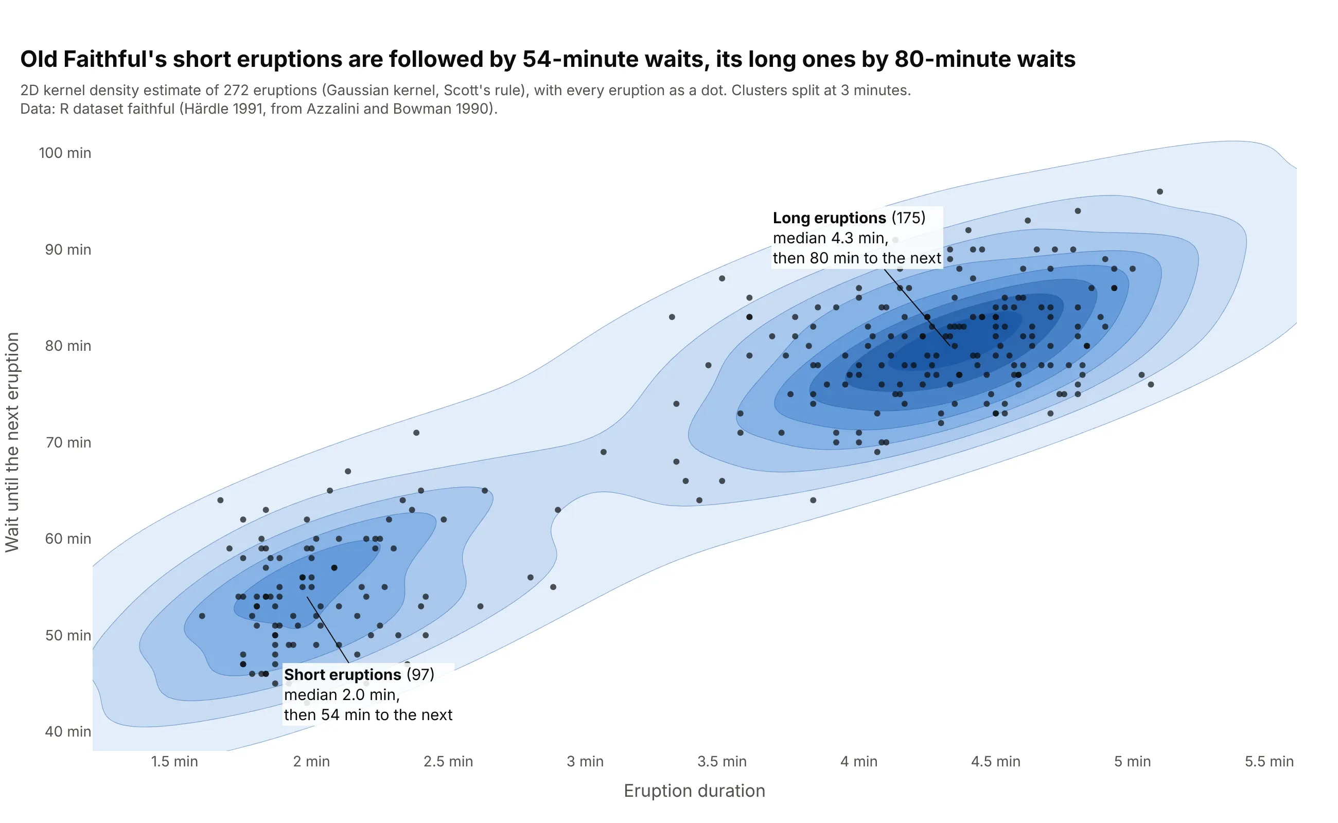
Short eruptions are followed by a median wait of 54 minutes and long ones by 80 minutes, so the length of one eruption predicts the next wait. This is the dataset seaborn's kdeplot documentation uses for its 2D examples. Data: R dataset faithful (Azzalini and Bowman 1990).
Tip: draw the dots on top of the filled contours, so the reader sees how few points some contours rest on.
Get the data from R's built-in faithful dataset (272 Old Faithful eruptions, from Azzalini and Bowman 1990)(columns: eruptions, waiting).Build a plotly 2D density plot: a 2D Gaussian KDE with scipy.stats.gaussian_kde on both columns, evaluatedon a 160 x 160 grid and drawn with go.Contour in filled blues, the eruptions as small dark dots on top, andeach cluster's median duration and wait labeled.
2. Daily moves in 2-year and 10-year Treasury yields
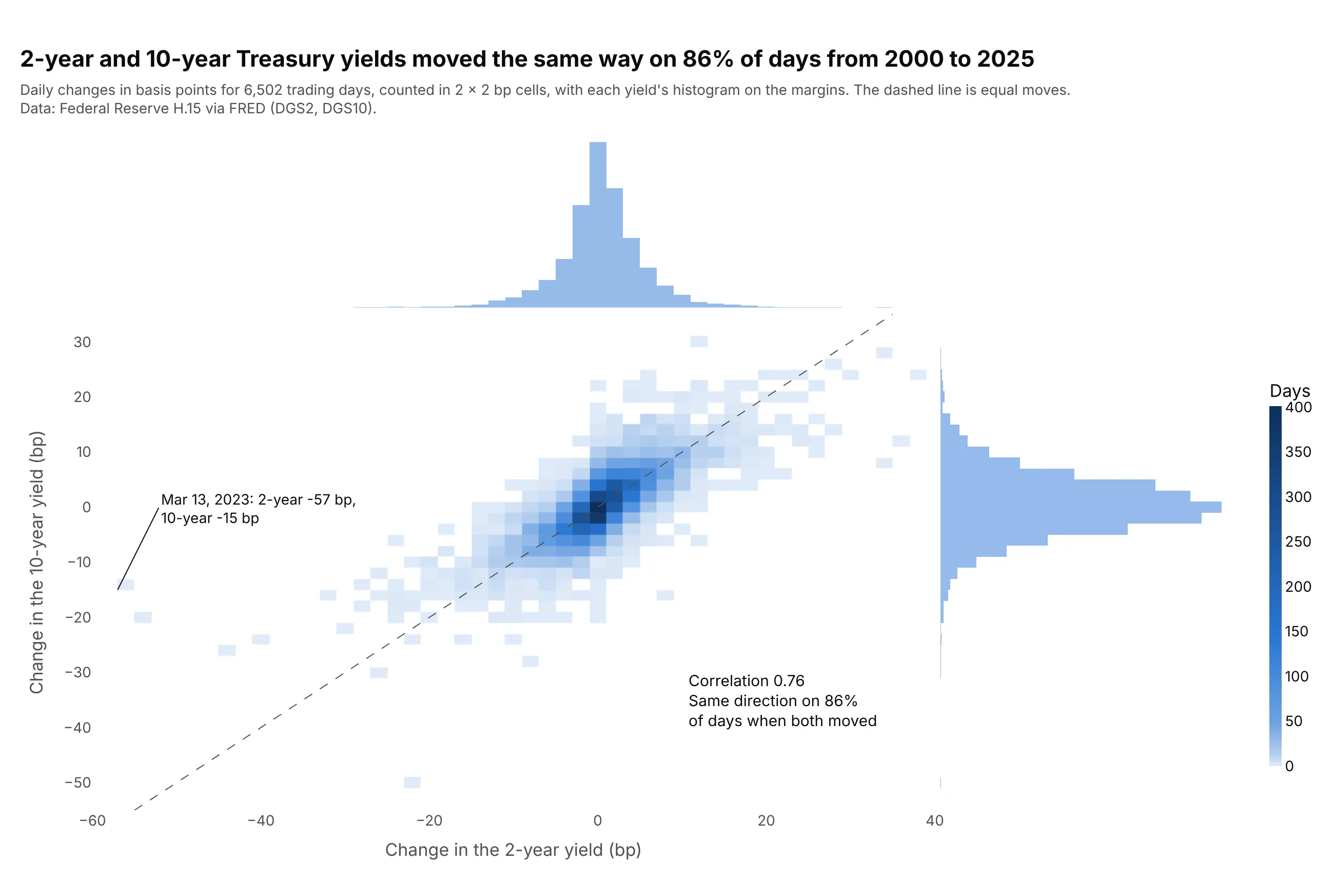
On days when both yields changed, they moved in the same direction 86% of the time, with a correlation of 0.76. The largest 2-year drop, 57 basis points on March 13, 2023, came with only a 15 bp fall in the 10-year. Data: Federal Reserve H.15 via FRED (DGS2, DGS10).
Tip: with whole-basis-point data, set the bins to exactly 2 bp so every cell holds the same number of possible values.
Get the data from the Federal Reserve's H.15 release (FRED series DGS2 and DGS10), daily 2000-2025, andcompute daily changes in basis points (columns: date, d2y_bp, d10y_bp).Build a plotly 2D density plot with px.density_heatmap: 2 x 2 bp bins, marginal histograms on both axes,a dashed line where both yields move equally, and the largest 2-year move labeled with its date.
3. German power prices in 2019 and 2025
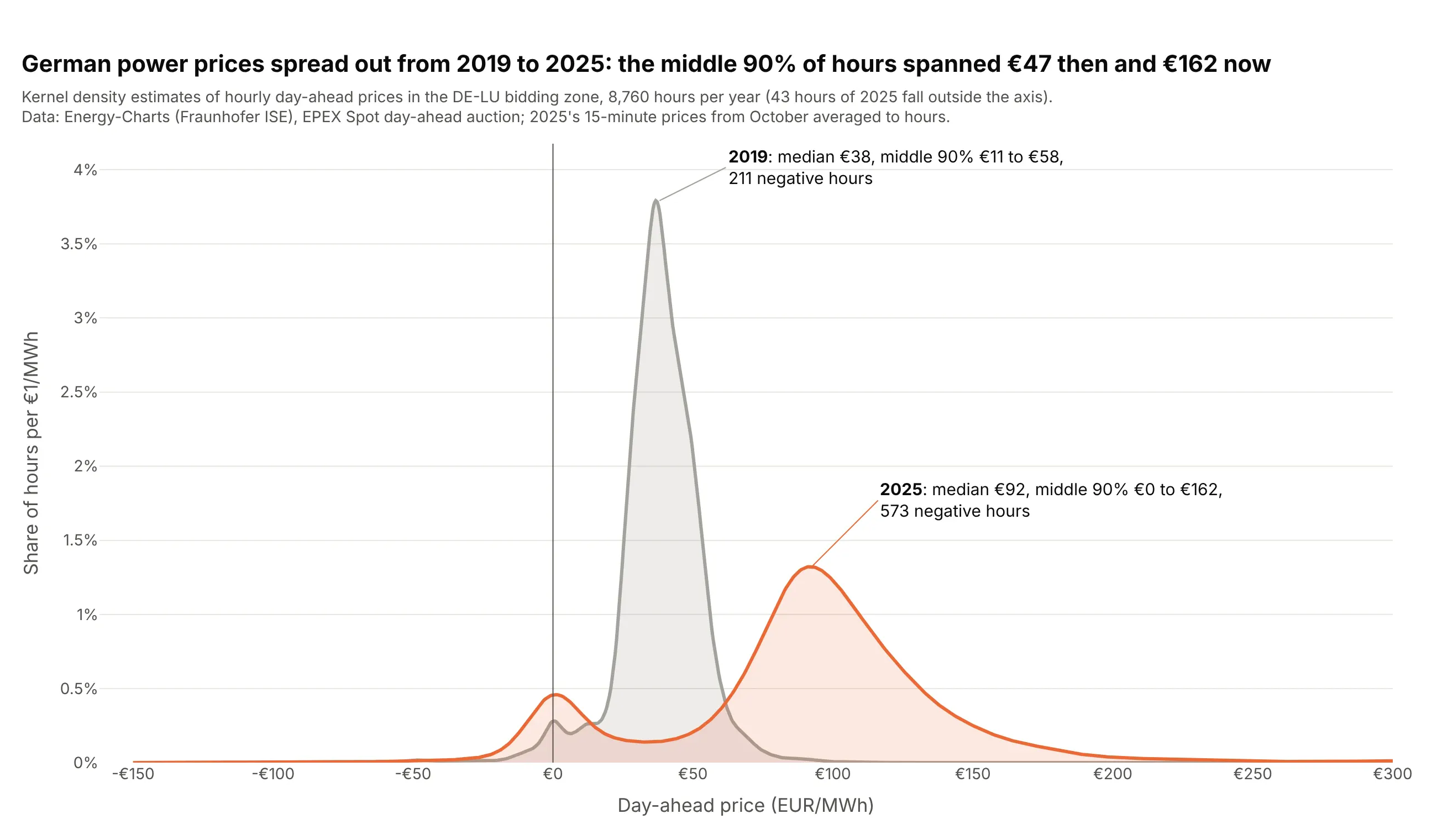
The middle 90% of hourly prices spanned €47 per MWh in 2019 and €162 in 2025, and the number of hours below zero went from 211 to 573. The 2025 curve also has a second bump at about €0. Data: Energy-Charts (Fraunhofer ISE), EPEX Spot day-ahead prices for the DE-LU bidding zone.
Tip: put a vertical line at zero so the negative-price hours are easy to compare between the two curves.
Get the data from the Energy-Charts API (Fraunhofer ISE, api.energy-charts.info, price endpoint) for theDE-LU bidding zone, 2019 and 2025, averaged to hourly prices (columns: year, hour, price_eur_mwh).Build a plotly density plot: one Gaussian KDE per year with scipy, drawn with go.Scatter and light fills,x from -150 to 300 EUR/MWh, a line at zero, and each year's median and number of negative hours labeled.
4. Clinical trial sizes by phase
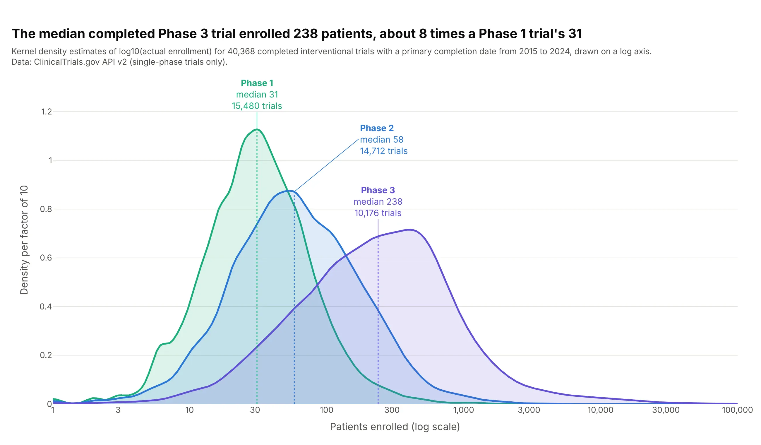
The median completed Phase 3 trial enrolled 238 patients, about 8 times a Phase 1 trial's 31, and the Phase 3 curve has a long right tail out to tens of thousands. The estimate is computed on the logarithm of enrollment, so each curve is smooth across four orders of magnitude. Data: ClinicalTrials.gov API v2, completed interventional trials with a primary completion date in 2015-2024.
Tip: compute the KDE on np.log10(values) and plot it against 10 ** grid on a log axis, rather than smoothing the raw counts.
Another way to see it: the same three curves as a ridgeline, one row per phase, so none of them hides another:
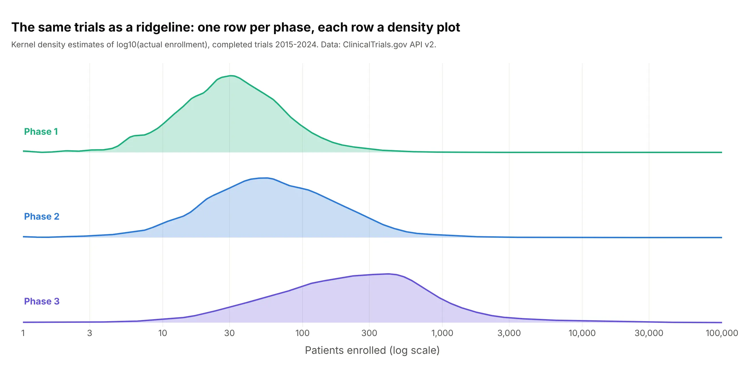
Get the data from the ClinicalTrials.gov API v2: completed interventional trials with a primary completiondate from 2015 to 2024, single-phase Phase 1, 2 or 3, with an actual enrollment (columns: nct_id, phase,enrollment).Build a plotly density plot: one Gaussian KDE per phase computed on log10(enrollment), drawn on a log xaxis from 1 to 100,000 with light fills, and each phase's median marked with a dotted line and labeled.
5. High cholesterol in US adults, then and now
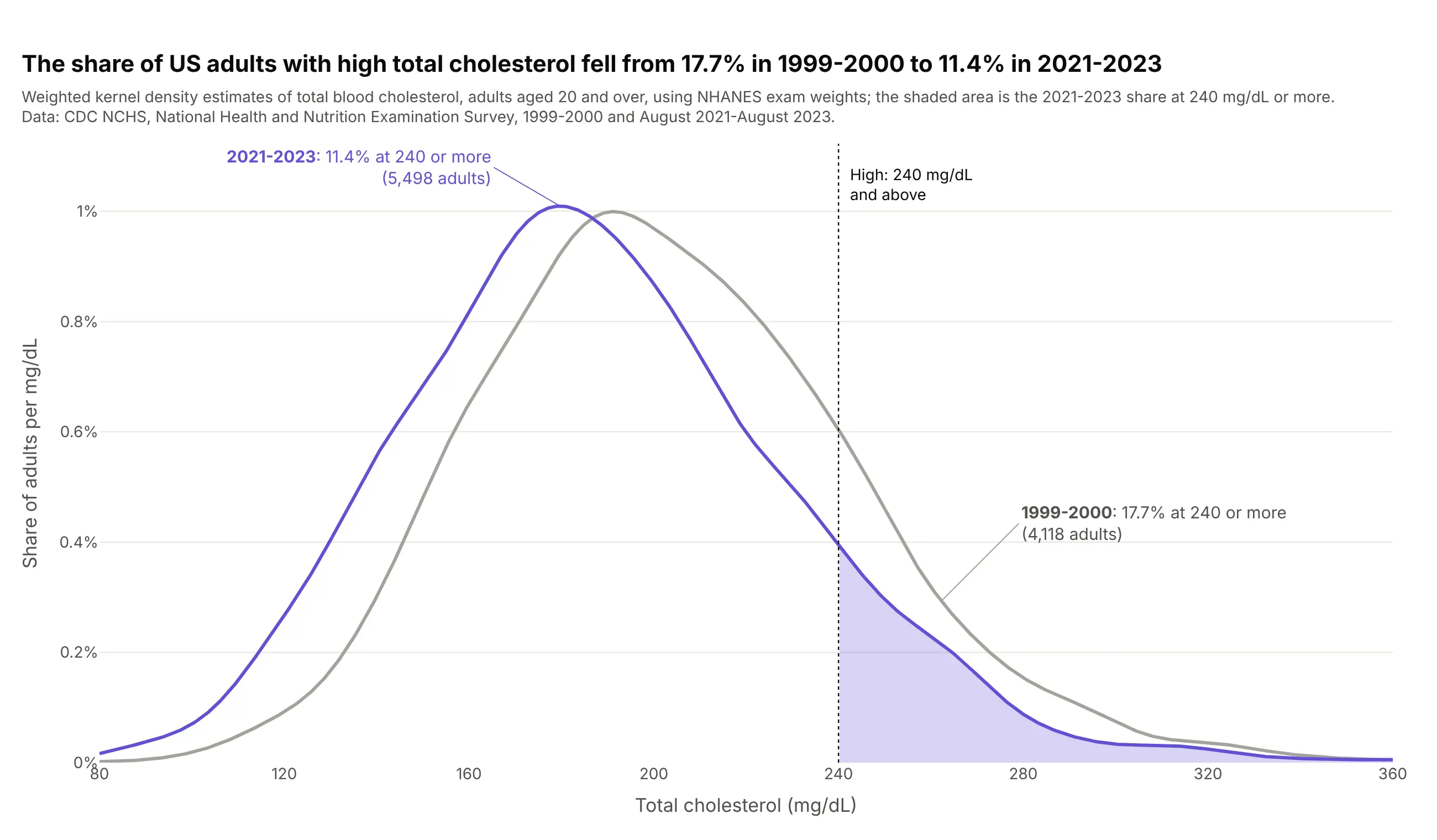
The share of US adults with total cholesterol of 240 mg/dL or more fell from 17.7% in 1999-2000 to 11.4% in 2021-2023, and the whole curve moved left. The curves use NHANES survey weights, and the result is close to the 11.3% in NCHS's own data brief. Data: CDC NCHS, NHANES 1999-2000 and August 2021-August 2023.
Tip: pass the survey weights to gaussian_kde(..., weights=...), and shade the area past the threshold so the share has a shape.
Get the data from CDC's National Health and Nutrition Examination Survey: total cholesterol (LBXTC) andexam weights (WTMEC2YR) for adults 20 and over, 1999-2000 (LAB13, DEMO) and 2021-2023 (TCHOL_L, DEMO_L)(columns: survey, age, tchol_mg_dl, weight).Build a plotly density plot: one weighted Gaussian KDE per survey, a dotted line at 240 mg/dL, the areaabove it shaded for 2021-2023, and each survey's weighted share at 240 or more in its label.
6. Where NBA players shoot from
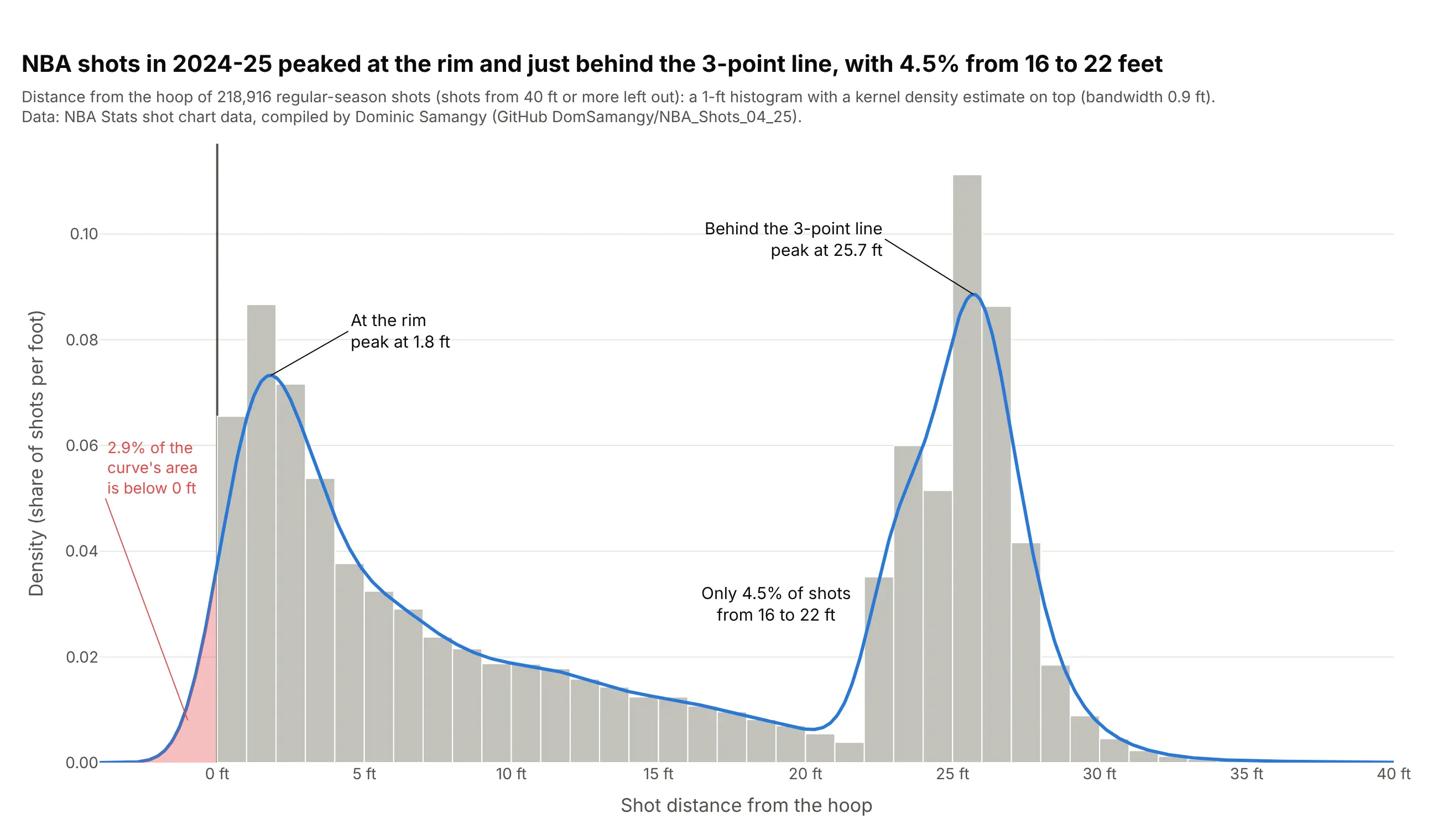
NBA shots in 2024-25 peaked at the rim and just behind the 3-point line, and only 4.5% came from 16 to 22 feet. The curve also shows the boundary problem: 2.9% of its area falls below 0 feet, where no shot can be. Data: NBA Stats shot chart data, compiled by Dominic Samangy (GitHub DomSamangy/NBA_Shots_04_25).
Tip: to match seaborn's histplot(kde=True), set the histogram's histnorm="probability density" so the bars and the curve share one y axis.
Get the data from NBA Stats shot chart data for the 2024-25 regular season (compiled per season in theGitHub repository DomSamangy/NBA_Shots_04_25) and compute each shot's distance from the hoop(columns: distance_ft, three, made).Build a plotly histogram with a density curve: 1-ft bins with histnorm="probability density" in light gray,a Gaussian KDE line on top, both peaks labeled, and the part of the curve below 0 ft shaded.
7. The standard sizes of US wind turbines
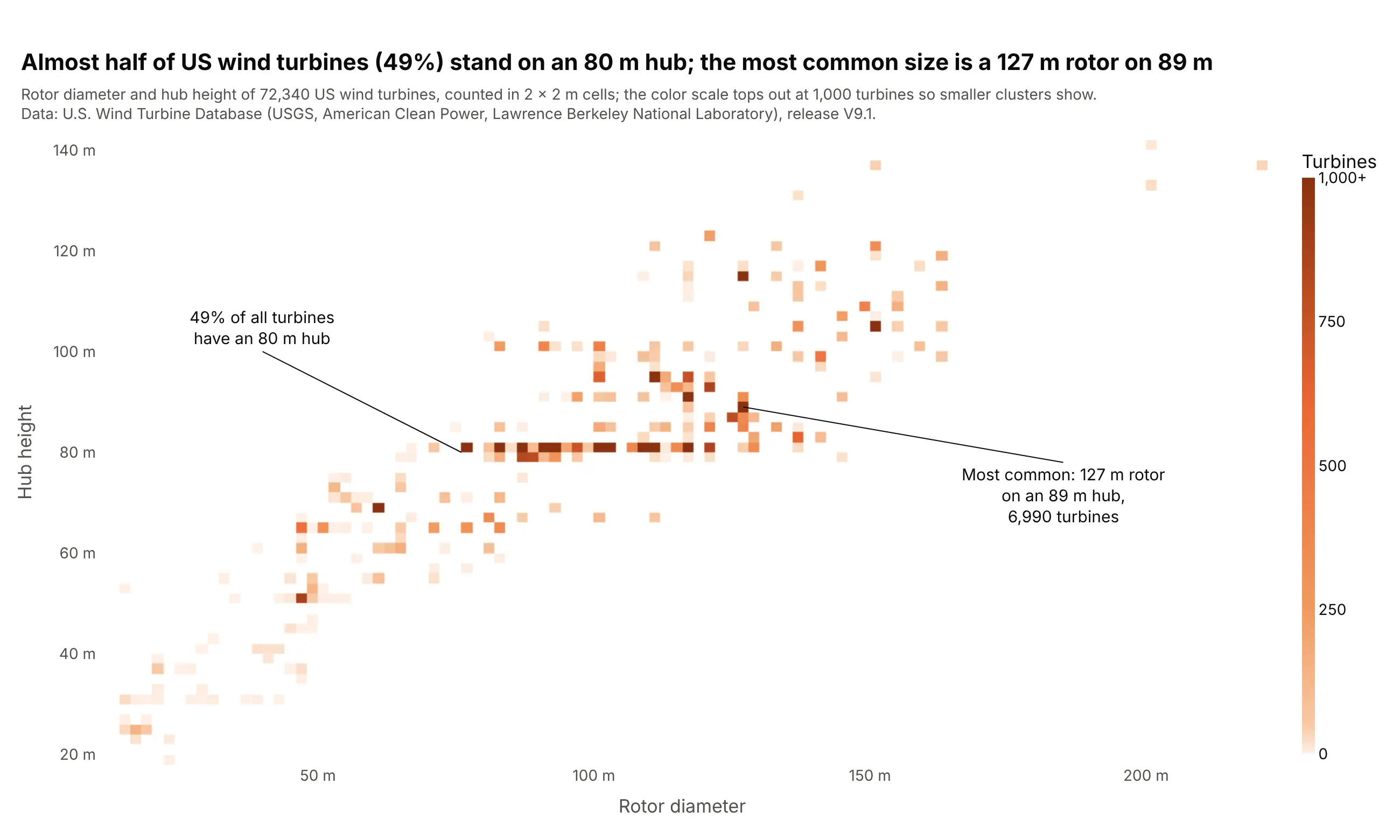
Almost half of US wind turbines (49%) stand on an 80 m hub, and the single most common size is a 127 m rotor on an 89 m hub, with 6,990 turbines. Thousands of identical turbines stack on the same point, which a scatter plot would draw as one dot. Data: U.S. Wind Turbine Database (USGS, American Clean Power, Lawrence Berkeley National Laboratory), release V9.1.
Tip: cap the color scale with range_color so a few huge cells don't wash out everything else, and say so in the subtitle.
Get the data from the U.S. Wind Turbine Database (USGS, American Clean Power and Lawrence Berkeley NationalLaboratory), every turbine with a rotor diameter and hub height (columns: rotor_m, hub_m, year, capacity_kw).Build a plotly 2D density plot with px.density_heatmap: 2 x 2 m bins, an orange color scale capped at1,000 turbines, and the most common rotor and hub combination labeled with its count.