Chris Parmer

October 24, 2026

Violin Plots - A Complete Guide

TL;DR

A violin plot compares the distribution of a number across groups. Each violin is a smoothed histogram mirrored around a center line, so it is wide where values are common and thin where they are rare.
Use one when groups have hundreds or thousands of values and the shape matters, such as two peaks, a long tail or a hard floor that a box plot would hide.
Use a strip plot instead for groups under about 30 values, and a histogram when one distribution and exact counts are the question.
Any coding agent can make one with Plotly in a minute. In Python it's px.violin(df, x="group", y="value", box=True).

What is a violin plot?

Violin plots look like this:

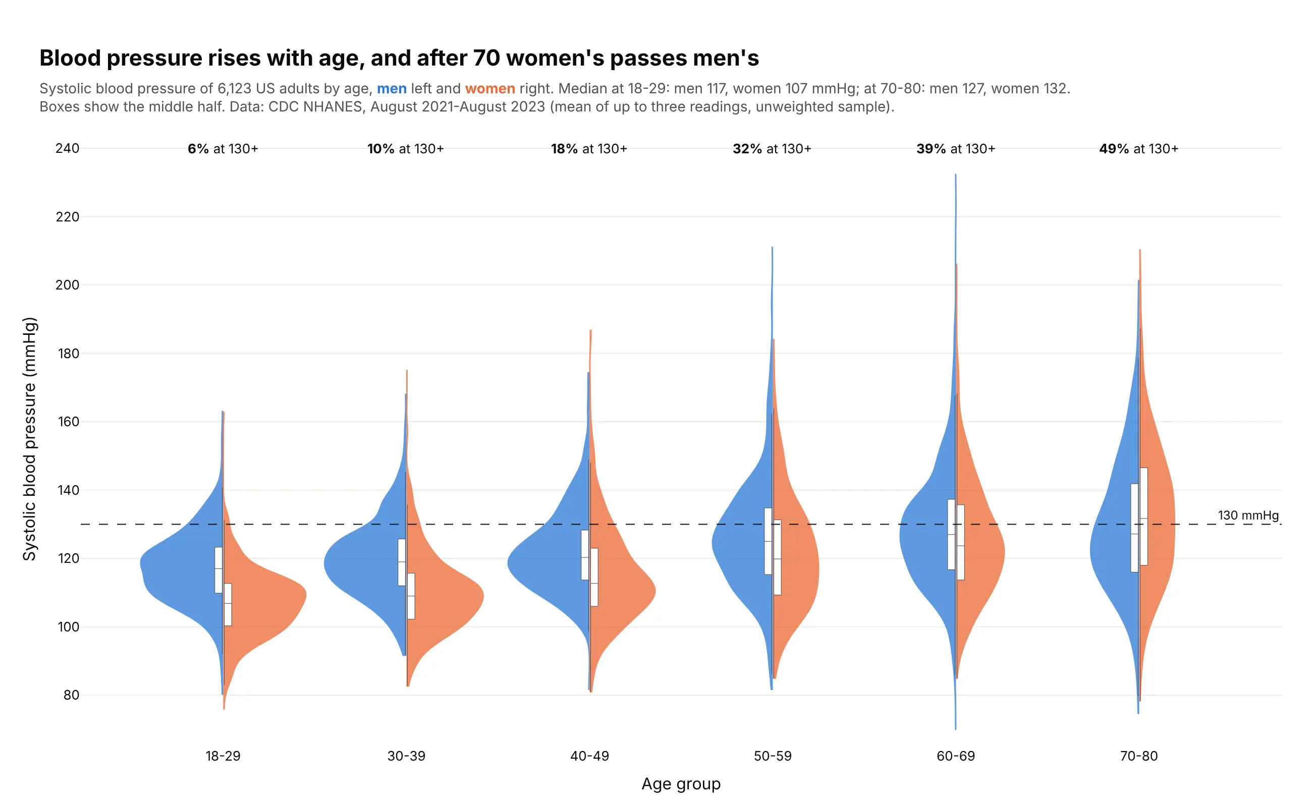
Split violins of systolic blood pressure for 6,123 US adults by age group, men in blue on the left and women in orange on the right, with a dashed line at 130 mmHg. The share at 130 or more rises from 6% at 18-29 to 49% at 70-80, and women's median passes men's after 70

Data: CDC NHANES, August 2021-August 2023.

How do you read a violin plot? In the example above, notice these things:

Each age group is one violin, split down the middle with men in blue on the left and women in orange on the right, and its height on the axis is systolic blood pressure.
The width of a violin at any height shows how many people had that reading, so the widest part is the most common blood pressure. For women aged 18-29 the bulk of the violin sits well below the dashed stage 1 hypertension line, and only 2% of them reached it.
The small white box inside each half shows the middle half of the readings, and the line across it is the median. In the 70-80 group the women's box sits higher than the men's, while in every younger group it sits lower.
From left to right the violins move up and stretch out, so blood pressure rises and varies more with age. The labels along the top show the share at 130 mmHg or more climbing with them.
A thin tail is only a few people with extreme readings. The tall blue spike in the 60-69 group comes from just four men at 200 mmHg or more, so it shows how far the range goes but carries little weight. Look at the wide parts and the boxes before the tails.

It's often used for charts like these:

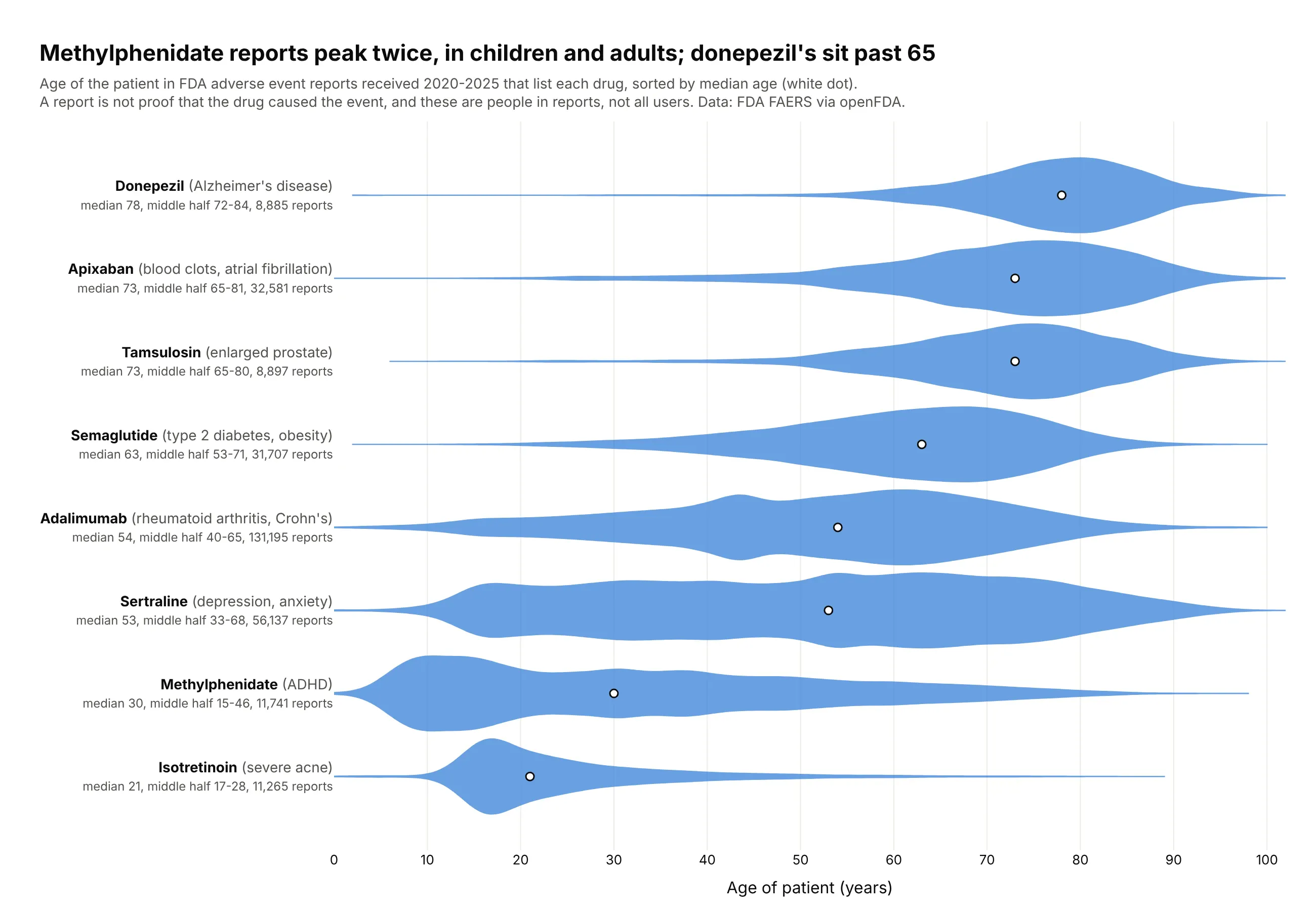
Horizontal violins of patient age in FDA adverse event reports from 2020-2025 for eight drugs, sorted by median: isotretinoin 21, methylphenidate 30 with peaks in childhood and adulthood, sertraline 53, adalimumab 54, semaglutide 63, tamsulosin 73, apixaban 73 and donepezil 78

Who a drug's patients are. Methylphenidate's reports have two peaks, children and adults, which a median of 30 would hide, while donepezil's sit almost entirely past 65 (median 78). Data: FDA FAERS via openFDA, reports received 2020-2025.

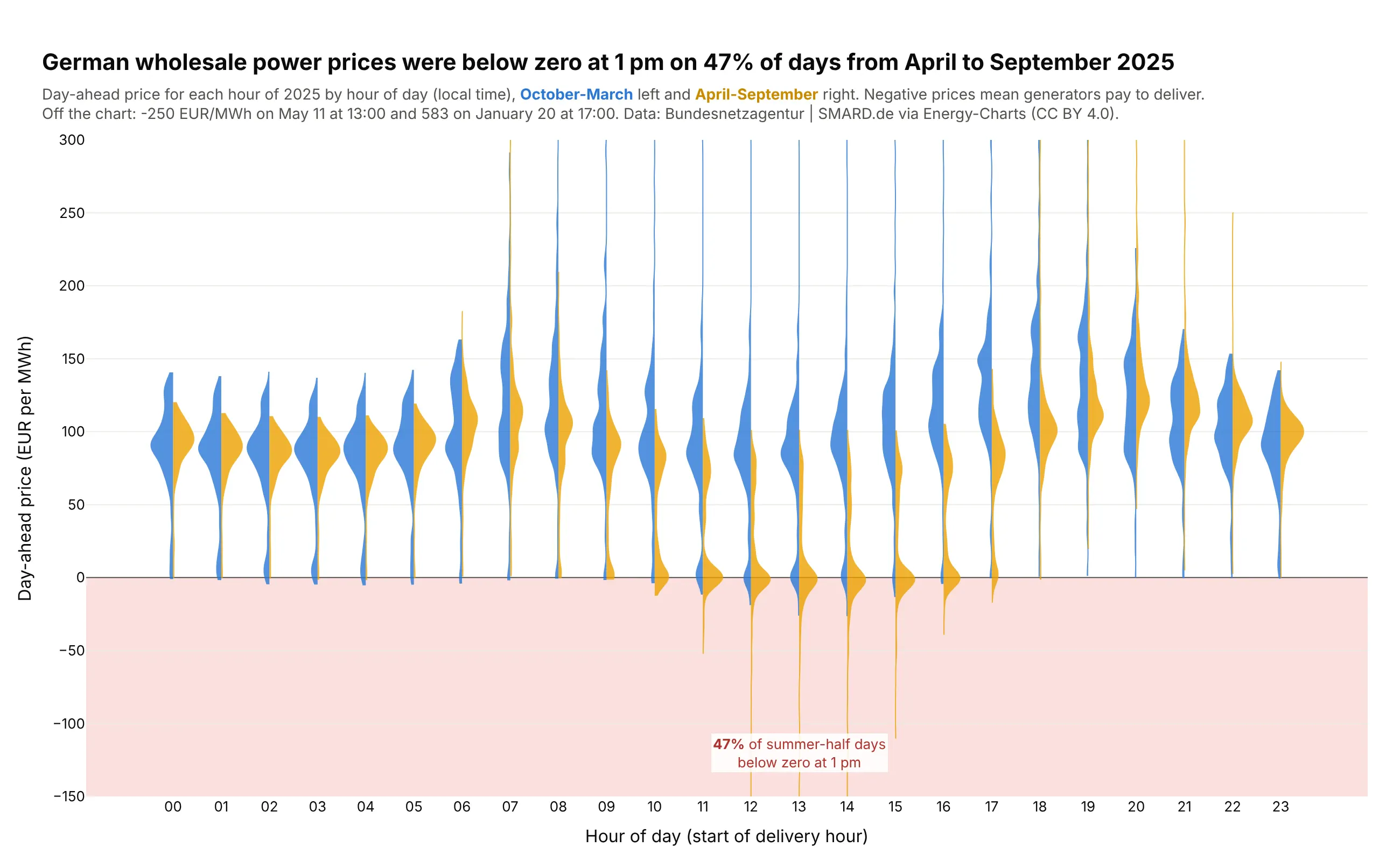
Split violins of German day-ahead prices for each hour of 2025, October-March on the left in blue and April-September on the right in yellow. Midday summer hours stretch far below zero, with 47% of April-September days negative at 1 pm

Power prices by hour. German wholesale power cost less than zero at 1 pm on 47% of days from April to September 2025, when solar floods the market, against 7% of days from October to March. Data: Bundesnetzagentur | SMARD.de via Energy-Charts.

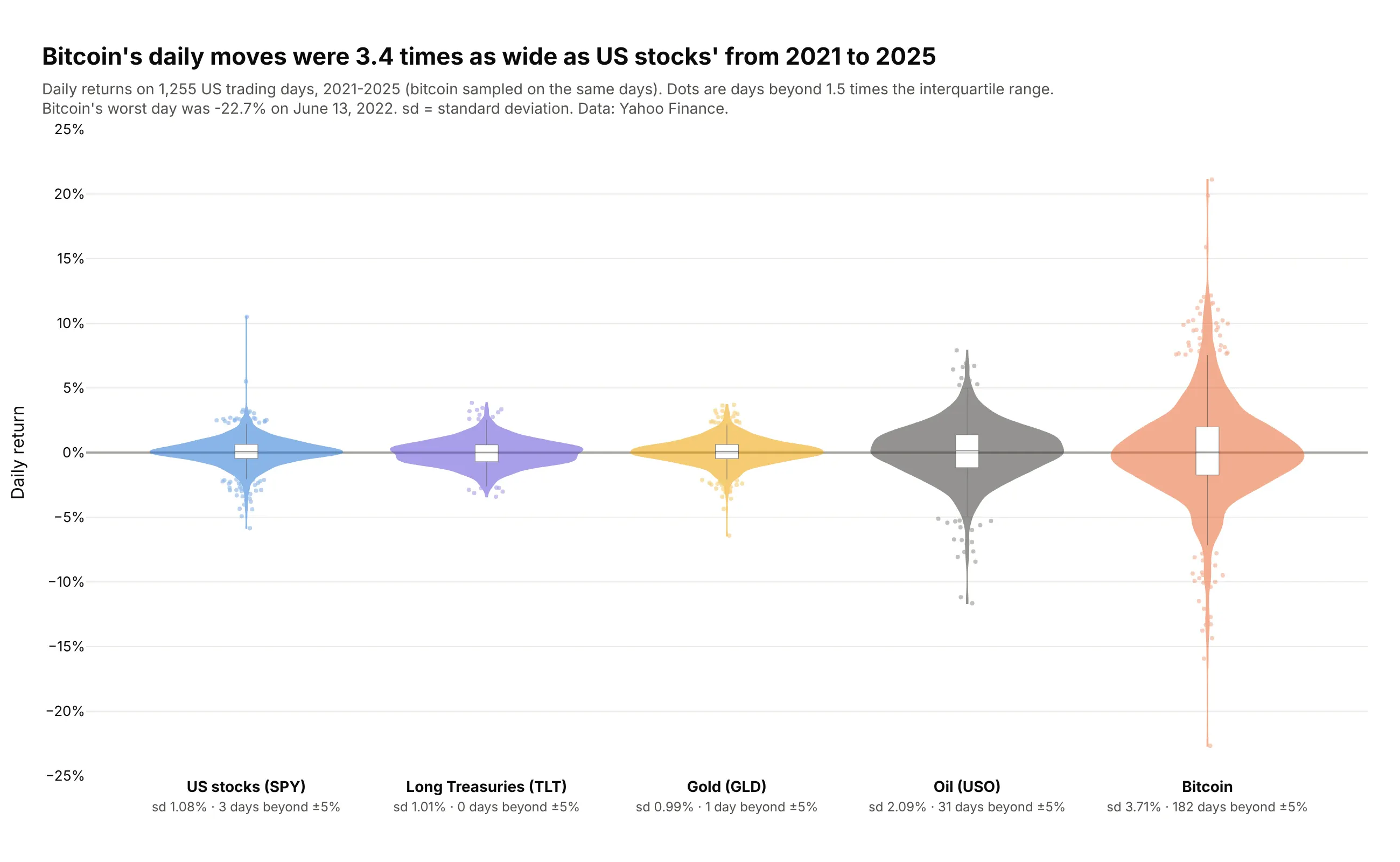
Violins of daily returns from 2021 to 2025 for SPY, TLT, GLD, USO and bitcoin with outlier days as dots. Bitcoin's standard deviation is 3.71% with 182 days beyond ±5%, against 1.08% and 3 days for SPY

Risk across assets. Bitcoin's daily returns from 2021 to 2025 were 3.4 times as spread out as the S&P 500 fund's, with 182 days beyond ±5% against 3. Data: Yahoo Finance, SPY, TLT, GLD, USO and BTC-USD.

A short history

Jerry Hintze and Ray Nelson introduced the violin plot in 1998 in The American Statistician as "a box plot-density trace synergism" (doi:10.1080/00031305.1998.10480559), adding a density estimate on both sides of a box plot. One of their examples put a box plot of Old Faithful's eruption lengths next to a violin, and here is that pair redrawn on the public version of the data:

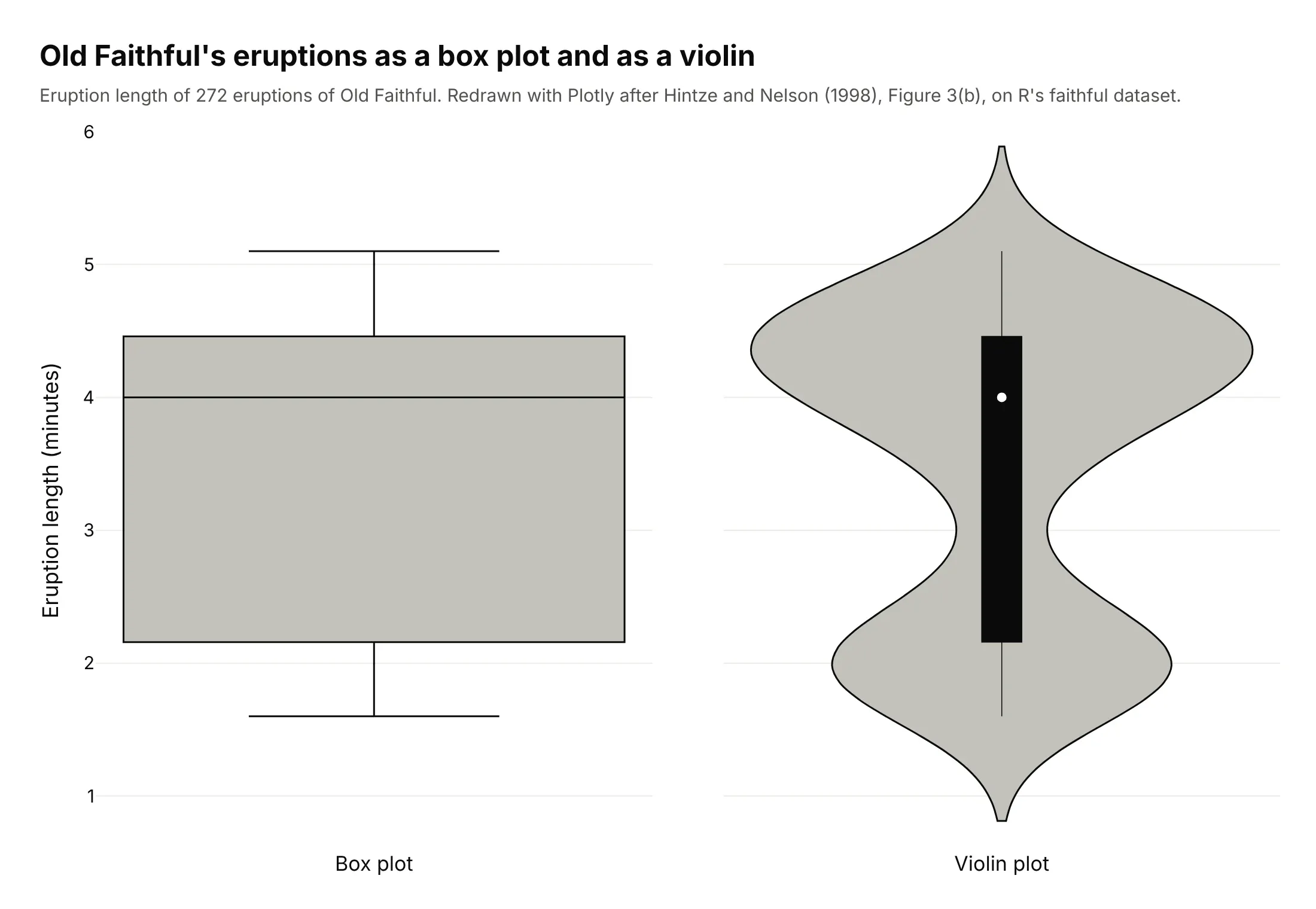
A box plot and a violin plot of the length of 272 eruptions of Old Faithful, redrawn with Plotly after Hintze and Nelson's 1998 Figure 3(b). The box plot shows a median of 4.0 minutes and a box from 2.2 to 4.5 minutes, while the violin shows two clusters, short eruptions around 2 minutes and long ones around 4.3 minutes, with almost none near 3

The box plot gives a median of 4.0 minutes and a box from 2.2 to 4.5, which suggests eruptions spread evenly across that range. The violin shows two separate kinds of eruption instead: 97 of the 272 were shorter than 3 minutes (median 2.0) and the rest longer (median 4.3). Half violins stacked with overlap later became popular as ridgeline plots through Claus Wilke's ggridges package for R in 2017.

Alternatives to a violin plot

Here's the same set of patient ages drawn six ways. Some are better for the question, some worse, some just different:

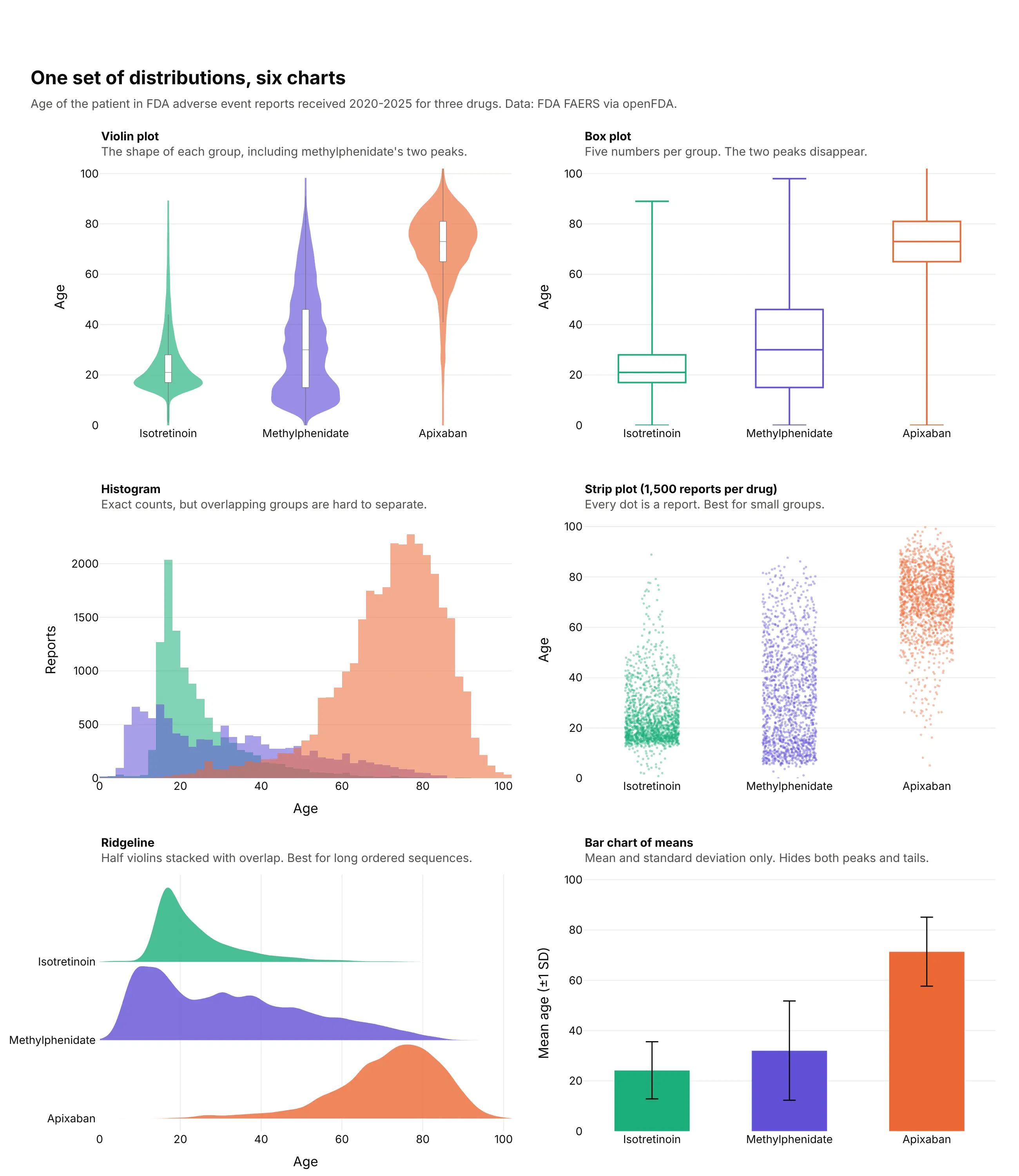
The ages of patients in FDA adverse event reports for isotretinoin, methylphenidate and apixaban drawn six ways: violins that show methylphenidate's two peaks, box plots that hide them, overlapping histograms, a strip plot of 1,500 reports per drug, a ridgeline and a bar chart of mean age with standard deviation bars

Box plot (works too, when the shape is simple). Five numbers per group are compact and precise about the median, and they hide methylphenidate's two peaks. See our box plot guide.
Histogram (better for one distribution). It shows exact counts and is the most honest view of a single group, but three overlapping histograms are hard to tell apart. See our histogram guide.
Strip plot (better for small groups). Every value is a dot, so nothing is smoothed away. Past a few hundred points per group the dots merge, which is why this one draws a sample.
Ridgeline (different). Half violins stacked with overlap, which suits a long ordered sequence such as 36 years or 24 hours. See our ridgeline plot guide.
Bar chart of means (worse). A mean and an error bar say nothing about peaks or tails. Correll and Gleicher (2014) found that readers misjudged data less often with violin and gradient plots than with bars and error bars.

How to make a violin plot

With AI

ChatGPT, Claude Code, GitHub Copilot, Cursor and other AI tools are excellent at writing Plotly code. Name Plotly in the prompt, describe the groups, the value and what to compare, and list the checks you want:

Make a plotly violin plot from trades.csv (columns: date, desk, pnl_usd).

- One violin per desk, sorted by median daily P&L; inner box; no points.
- If a desk has more than 20,000 rows, draw a random sample (seed 0) and say so in the subtitle,
  but compute medians and percentiles from all rows.
- spanmode="hard"; set one bandwidth for all desks and print the value you chose.
- Clip the y axis at the 0.5th and 99.5th percentiles and name the days off the chart in the subtitle.
- Inter font, white background, a title that states the takeaway with a real number.
- Save it as violins.html and as a PNG at 2x scale, and check the HTML is under 5 MB.

With Plotly Studio

Plotly Studio is a desktop app where you point an AI at a dataset and it builds charts and a Dash app around your questions. Ask for a violin plot the same way:

Show violin plots of systolic blood pressure by age group, split by sex with men on the left and women on the right. Add an inner box, a dashed line at 130 mmHg and the share of each age group at or above it. Add a dropdown to switch between systolic and diastolic pressure.

Make a violin plot in Python or JavaScript

This is the code AI tools write under the hood. In Python, Plotly Express takes a long table with one row per value:

import plotly.express as px

df = px.data.tips()
fig = px.violin(df, x="day", y="total_bill", color="sex", box=True, points=False,
                category_orders={"day": ["Thur", "Fri", "Sat", "Sun"]})
fig.update_traces(side="positive", selector=dict(name="Female"))
fig.update_traces(side="negative", selector=dict(name="Male"))
fig.update_layout(violinmode="overlay", violingap=0)
fig.show()

Setting side on each trace and violinmode="overlay" turns the pairs into split violins. In JavaScript, plotly.js takes one trace per group or side:

<div id="chart"></div>
<script src="https://cdn.plot.ly/plotly-4.1.1.min.js"></script>
<script>
  const before = [118, 121, 125, 127, 129, 131, 132, 134, 138, 141, 145, 152];
  const after = [112, 115, 117, 119, 120, 122, 123, 125, 127, 130, 133, 139];
  Plotly.newPlot("chart", [
    {type: "violin", y: before, x0: "Systolic (mmHg)", name: "Before", side: "negative",
     box: {visible: true}, spanmode: "hard"},
    {type: "violin", y: after, x0: "Systolic (mmHg)", name: "After", side: "positive",
     box: {visible: true}, spanmode: "hard"}
  ], {violinmode: "overlay"});
</script>

The numbers in the JavaScript example are made up to keep it short.

Share it

Every Plotly chart has a Share chart button (the cloud icon in its toolbar) that uploads it to Plotly Cloud and gives you a link. Only you can see it until you change its visibility.

For a live app, put the chart in a Dash app and publish it with the Plotly Cloud CLI. Coding agents can run these commands for you:

pip install "dash[cloud]"
plotly user login
plotly app publish

If your data has to stay in your own cloud or data center, publish to Dash Enterprise instead.

Dos and don'ts

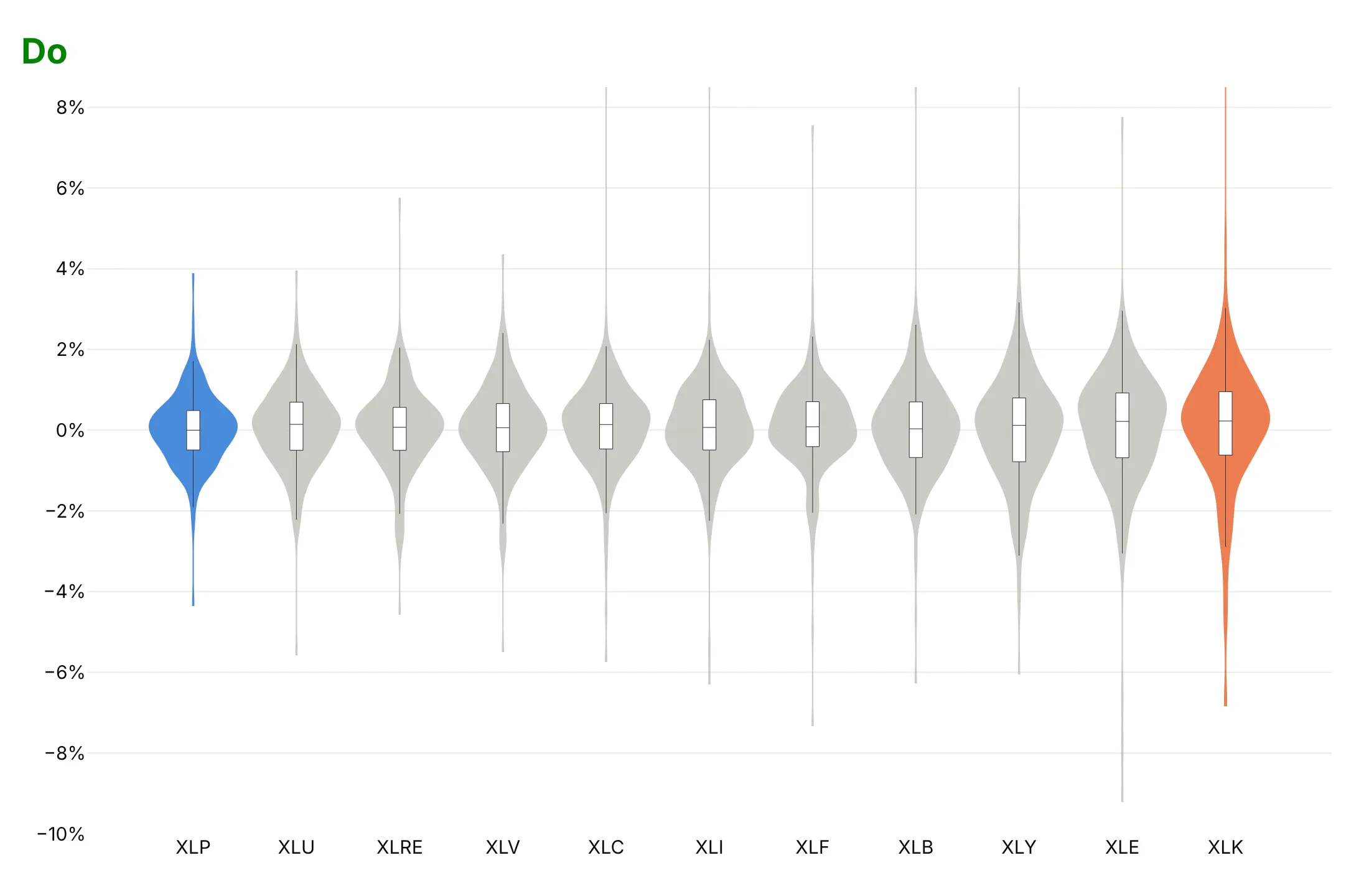
Both charts below show 250 days of 2025 sector fund returns with the same colors, gray with technology (XLK, orange) and consumer staples (XLP, blue) picked out, and the same inner boxes. They differ only in the mistakes.

Don't sort groups with no natural order alphabetically, leave the axis without units, let one extreme day set the range so every violin is squashed into the middle, or add a legend that repeats the axis labels:

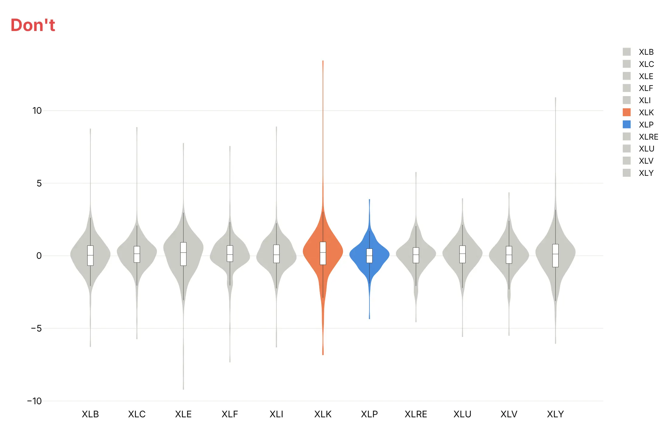
Violins of the daily returns of 11 sector funds in 2025, gray with technology in orange and consumer staples in blue, in alphabetical order, on a y axis from -10 to 15 with no percent sign, so the violins fill only the middle of the chart, and with a legend that repeats the tickers

Do sort by spread, put the unit on the axis, drop the legend and cut the axis at the extremes, then name what's off the chart in the text. Sorted, the chart shows that technology swung twice as much as consumer staples, and its +13.4% day on April 9 is above the cut:

The same violins sorted by daily standard deviation from consumer staples to technology, all gray except consumer staples in blue and technology in orange, with white inner boxes and the y axis cut at -10% and +8.5%

Four ways to draw the same violins

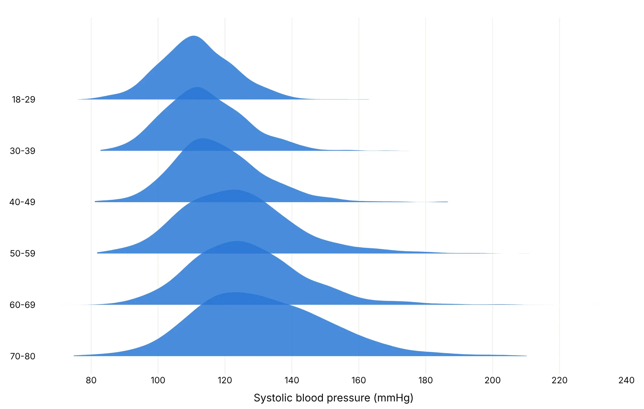
The same blood pressure data can be drawn four ways, and each one answers a different question.

With an inner box. The default for publishing, because readers who know box plots still get the median and quartiles.

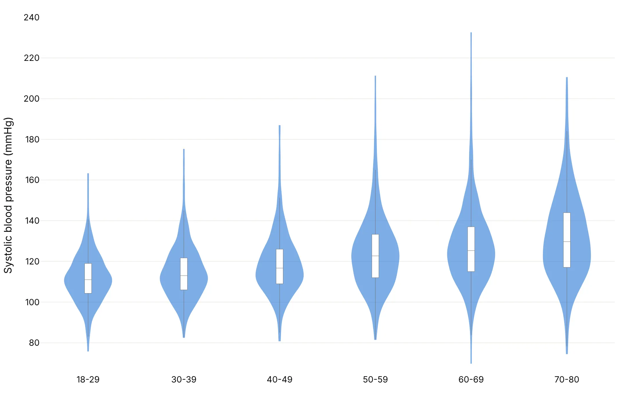
Violins of systolic blood pressure for 6,123 US adults by age group, each with a white inner box plot

With every point. Useful when groups are small or individual values matter. With 769 to 1,448 people per group here, the dots already start to merge.

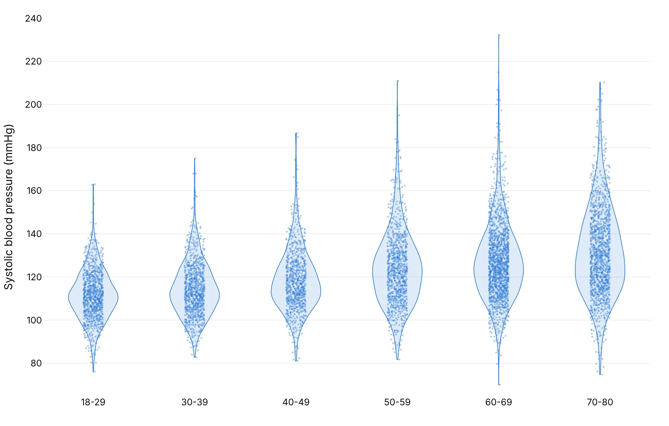
Violins of systolic blood pressure by age group drawn as light outlines with every person as a small blue dot

Split. Two subgroups back to back in one violin per group, here men on the left and women on the right.

Split violins of systolic blood pressure by age group, men in blue on the left and women in orange on the right

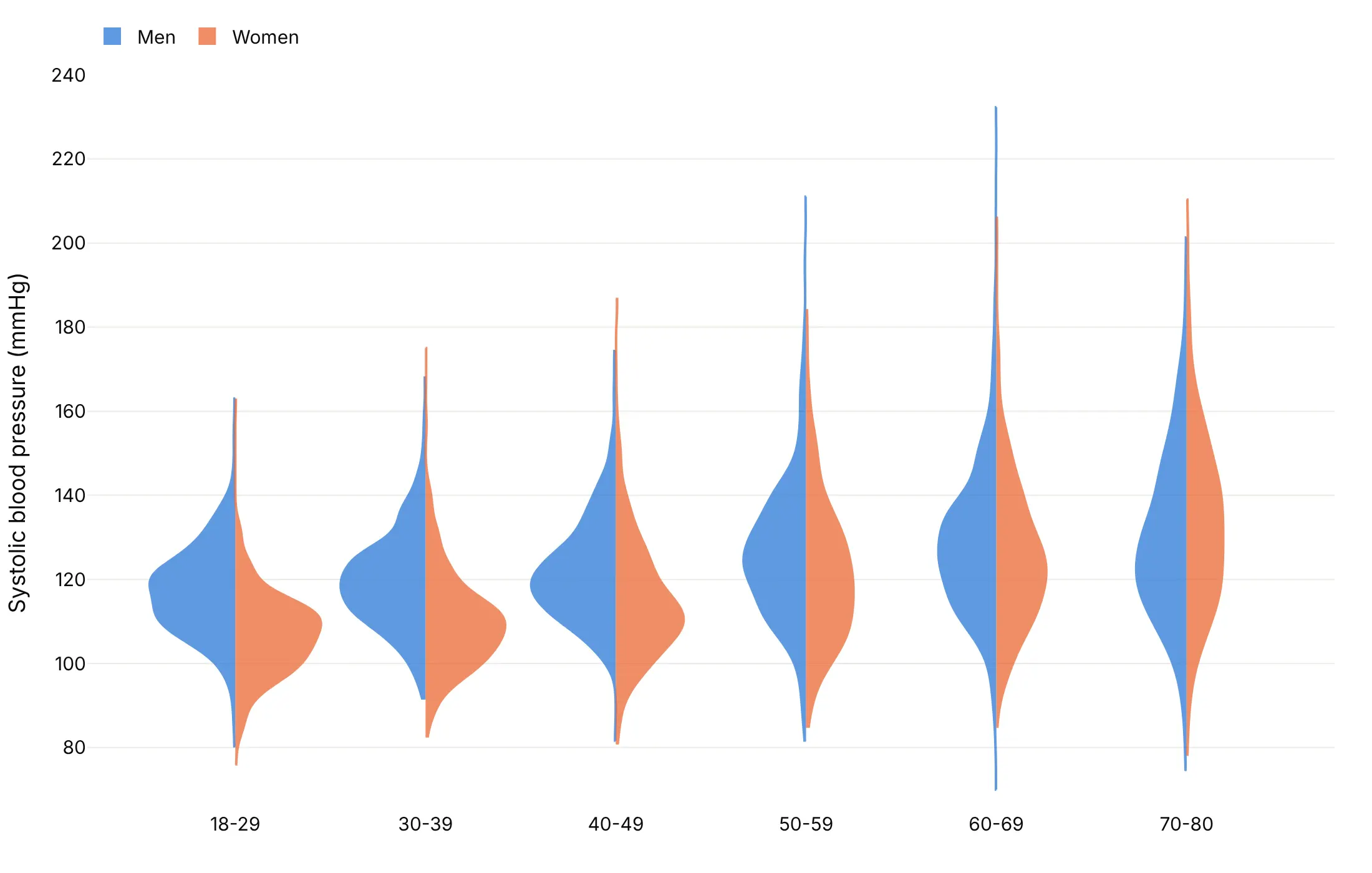
Ridgeline. Horizontal half violins that overlap, which read like a sequence from youngest to oldest.

A ridgeline of systolic blood pressure by age group, with one overlapping blue ridge per group from 70-80 at the bottom to 18-29 at the top

Choose the bandwidth on purpose

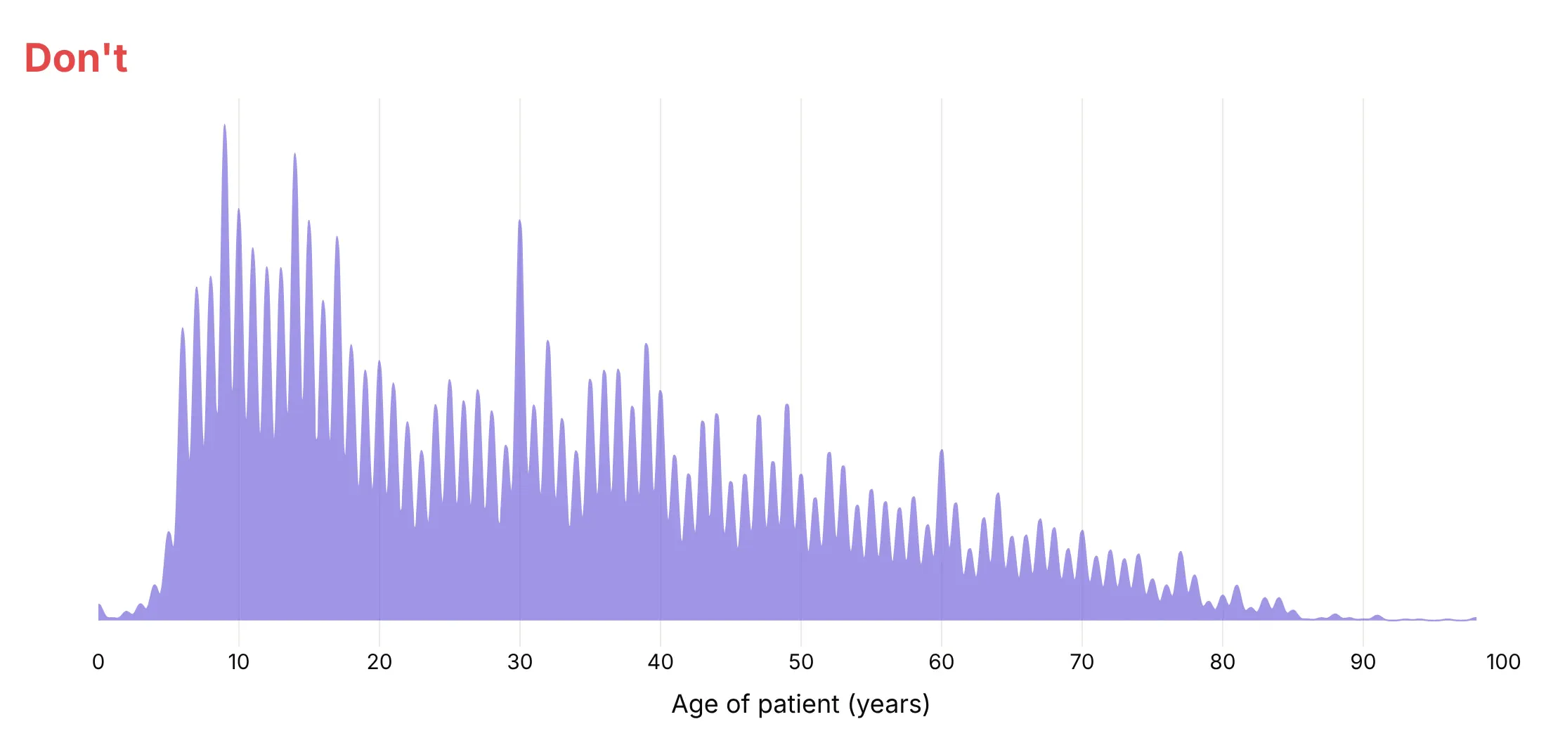
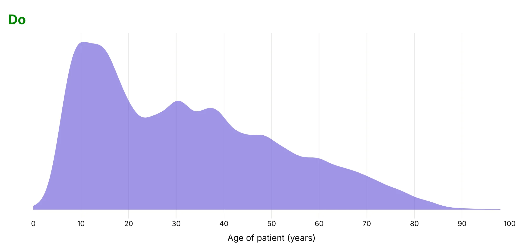
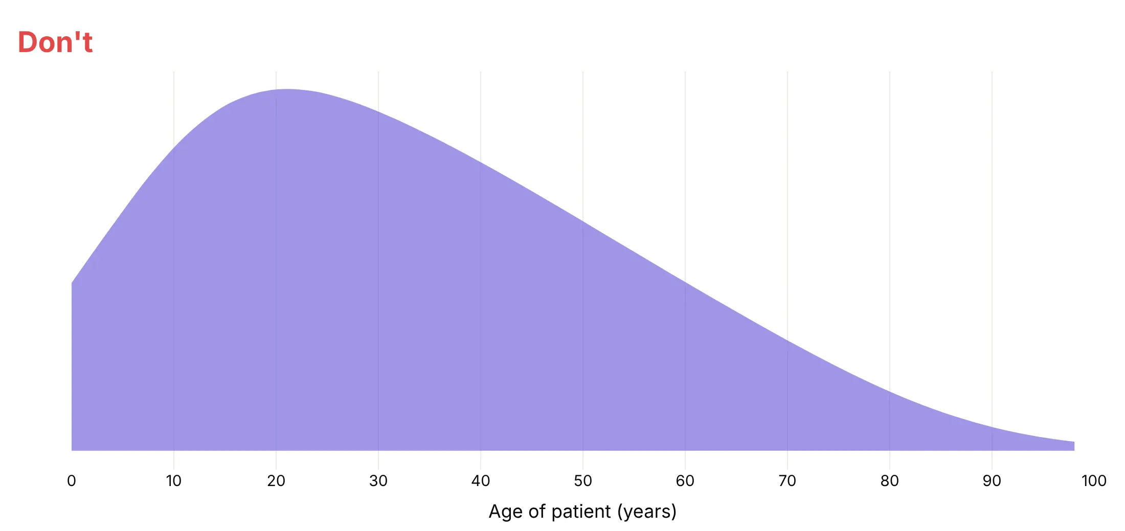
The bandwidth is how far each value is smeared when Plotly estimates the density. Plotly picks one per violin with Silverman's rule of thumb, about 3.2 years for these 11,741 methylphenidate patient ages, and you can set it with bandwidth.

Don't go below the rounding step of the data. Ages are whole years, so a bandwidth of 0.3 draws a spike at every year:

A half violin of 11,741 patient ages in methylphenidate adverse event reports with bandwidth 0.3, which draws a comb of spikes, one at every whole year

Do pick a value that shows the real structure. A bandwidth of 2 years shows the two peaks, children around 10 and adults around 30 to 40:

The same ages with bandwidth 2, a smooth shape with a tall peak around age 10 and a second, lower bump between 30 and 40

Don't smooth so much that real peaks merge. With a bandwidth of 12 years, the children and adults become one hump:

The same ages with bandwidth 12, a single wide hump from 0 to 100 with no separate peaks

Checklist

Write a title that states the takeaway.
Sort the groups by median or spread unless they have a natural order.
Keep the inner box (box_visible=True) so readers get the median and quartiles.
Stop the violins at the data with spanmode="hard".
Set the bandwidth yourself when values are rounded or the groups must be smoothed alike.
Cut extreme axes and name what's off the chart in the subtitle.

Don't

Draw every point on groups of thousands.
Use a violin for groups of 10 values; show the points.
Put raw values on a log axis; plot log10 values instead.
Color every violin differently when the colors mean nothing.

Options to customize

These are the go.Violin (and px.violin) options that matter most. The full list is in the Plotly violin documentation.

x, y, orientation: the values and group positions; orientation="h" for long labels and ridgelines.
x0 / y0, name: put a whole trace at one category, instead of a list that repeats the group name for every value.
box_visible, box_width: the inner box plot. Use it almost always.
meanline_visible: a line at the mean, for when mean and median differ.
points: "all", "outliers", "suspectedoutliers" or False. Use "all" for small groups and False for big ones.
pointpos, jitter, marker: where the points sit and how they spread.
side: "both", "negative" or "positive", for split violins and ridgelines.
bandwidth: the kernel width in data units (default: Silverman's rule). Set it for rounded data.
spanmode, span: where the outline stops: "soft", "hard" (the data range) or "manual". Use "hard" for data with natural limits.
scalemode, scalegroup: equal widths ("width") or widths by count ("count"), so rare groups look rare. Leave width unset with "count".
width: the maximum width of the trace; above 1 makes ridgelines overlap.
quartilemethod: "linear", "exclusive" or "inclusive", to match quartiles from another tool.
hoveron: "violins", "points" or "kde"; "kde" shows the density at the cursor.
violinmode, violingap, violingroupgap (layout): "overlay" for splits, "group" for violins side by side, and the spacing between them.

More violin plot examples

Ten more violin plots built from real public data, each with its source, the technique that makes it work and a prompt to rebuild it.

1. Every year of S&P 500 daily returns since 1990

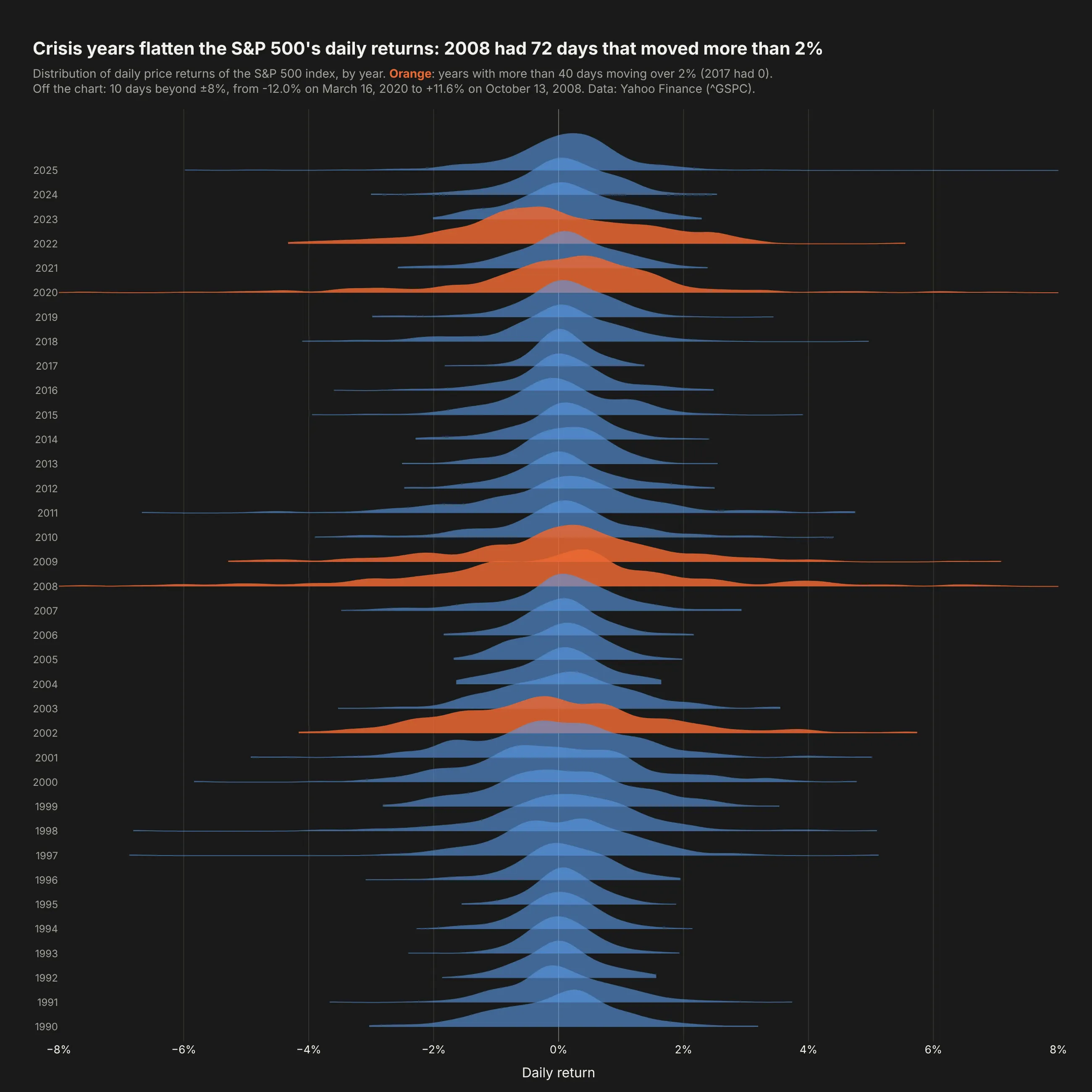
A dark ridgeline of S&P 500 daily return distributions for each year from 1990 to 2025. Calm years are tall narrow peaks; 2002, 2008, 2009, 2020 and 2022 are wide orange ridges, with 72 days moving more than 2% in 2008

Calm years are tall and narrow and crisis years are low and wide. 2008 had 72 days that moved more than 2%, and 2017 had none. Data: Yahoo Finance, S&P 500 index (^GSPC), 1990-2025.

Tip: a ridgeline is horizontal half violins: orientation="h", side="positive" and width=3 so each ridge overlaps the one above.

Get the data from Yahoo Finance daily closes for the S&P 500 index (^GSPC), 1989-12-29 to 2025-12-31,
and shape it into a table (columns: date, year, close, return_pct).

Build a plotly ridgeline: one horizontal violin per year, side="positive", width=3, newest at the top,
bandwidth 0.25, dark background. Color years with more than 40 days beyond ±2% orange.
Clip the x axis at ±8% and say how many days are off the chart.

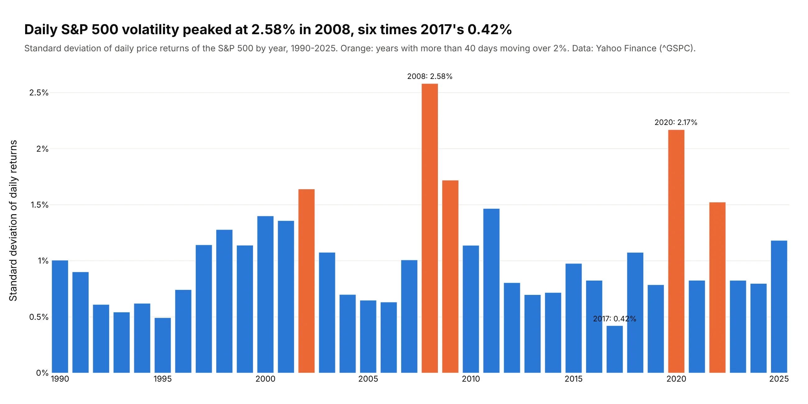
Another way to see it: one bar per year of the standard deviation is easier to rank (2.58% in 2008, six times 2017's 0.42%), but loses the tails.

Bar chart of the standard deviation of S&P 500 daily returns by year from 1990 to 2025, peaking at 2.58% in 2008 and 2.17% in 2020, with the lowest at 0.42% in 2017

2. HbA1c and the diabetes threshold

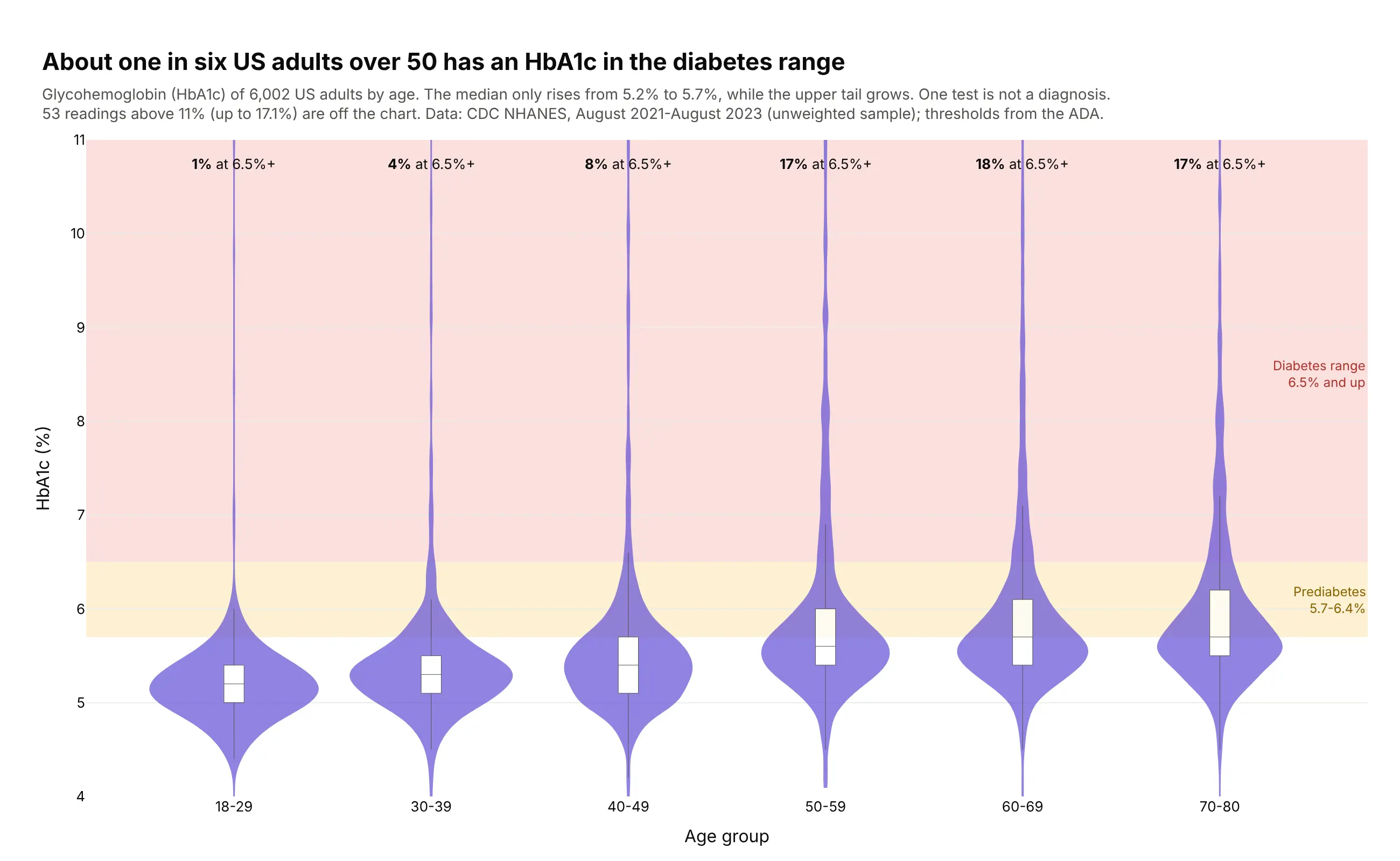
Violins of HbA1c for 6,002 US adults by age group over a yellow prediabetes band (5.7-6.4%) and a pink diabetes band (6.5%+). The share at 6.5% or more rises from 1% at 18-29 to 17-18% from age 50, while the median moves only from 5.2% to 5.7%

The median HbA1c barely moves with age (5.2% to 5.7%), but the upper tail grows, so 17-18% of adults over 50 are in the diabetes range, against 1% at 18-29. One test is not a diagnosis. Data: CDC NHANES, August 2021-August 2023.

Tip: threshold bands drawn with add_hrect(layer="below") turn the y axis into clinical categories without hiding the violins.

Get the data from CDC NHANES August 2021-August 2023 (DEMO_L and GHB_L files, wwwn.cdc.gov/nchs/nhanes)
and shape it into a table (columns: seqn, sex, age, age_group, hba1c) for adults 18+.

Build plotly violins of hba1c by age_group in one color, inner box, bandwidth 0.12, spanmode="hard".
Shade 5.7-6.4% (prediabetes) and 6.5%+ (diabetes range) behind the violins and print the share
at 6.5%+ above each group. Cut the y axis at 11% and say how many readings are above it.

3. Clinical trial enrollment by phase

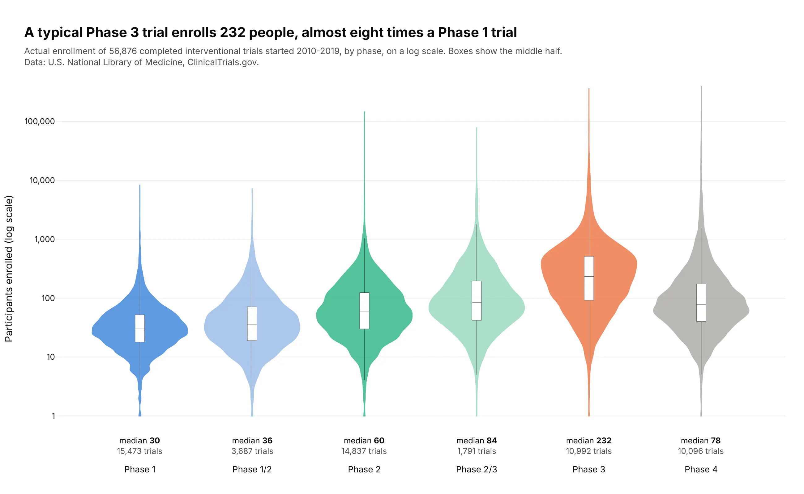
Violins of actual enrollment in 56,876 completed trials started 2010-2019 on a log scale by phase. Medians: Phase 1 30, Phase 1/2 36, Phase 2 60, Phase 2/3 84, Phase 3 232 and Phase 4 78

A typical Phase 3 trial enrolls 232 people, almost eight times a Phase 1 trial (30). Phase 4 trials are smaller at the median (78) but have the longest tail, up to 393,387 participants. Data: ClinicalTrials.gov, completed interventional trials started 2010-2019.

Tip: plot np.log10(enrollment) on a linear axis with tickvals and ticktext set to 1, 10, 100 and so on, because violins on a type="log" axis lose their shape.

Get the data from the ClinicalTrials.gov API v2 (clinicaltrials.gov/api/v2/studies): completed
interventional trials started 2010-2019 with a phase, and shape it into a table
(columns: nct_id, phase, enrollment [actual], start, primary_completion, sponsor_class).

Build plotly violins of log10(enrollment) by phase in phase order, inner box, spanmode="hard",
y ticks labeled 1, 10, 100, 1,000, 10,000, 100,000. Print the median and number of trials under
each phase. Title with the Phase 3 vs Phase 1 median.

4. What a year of one drug costs Medicare

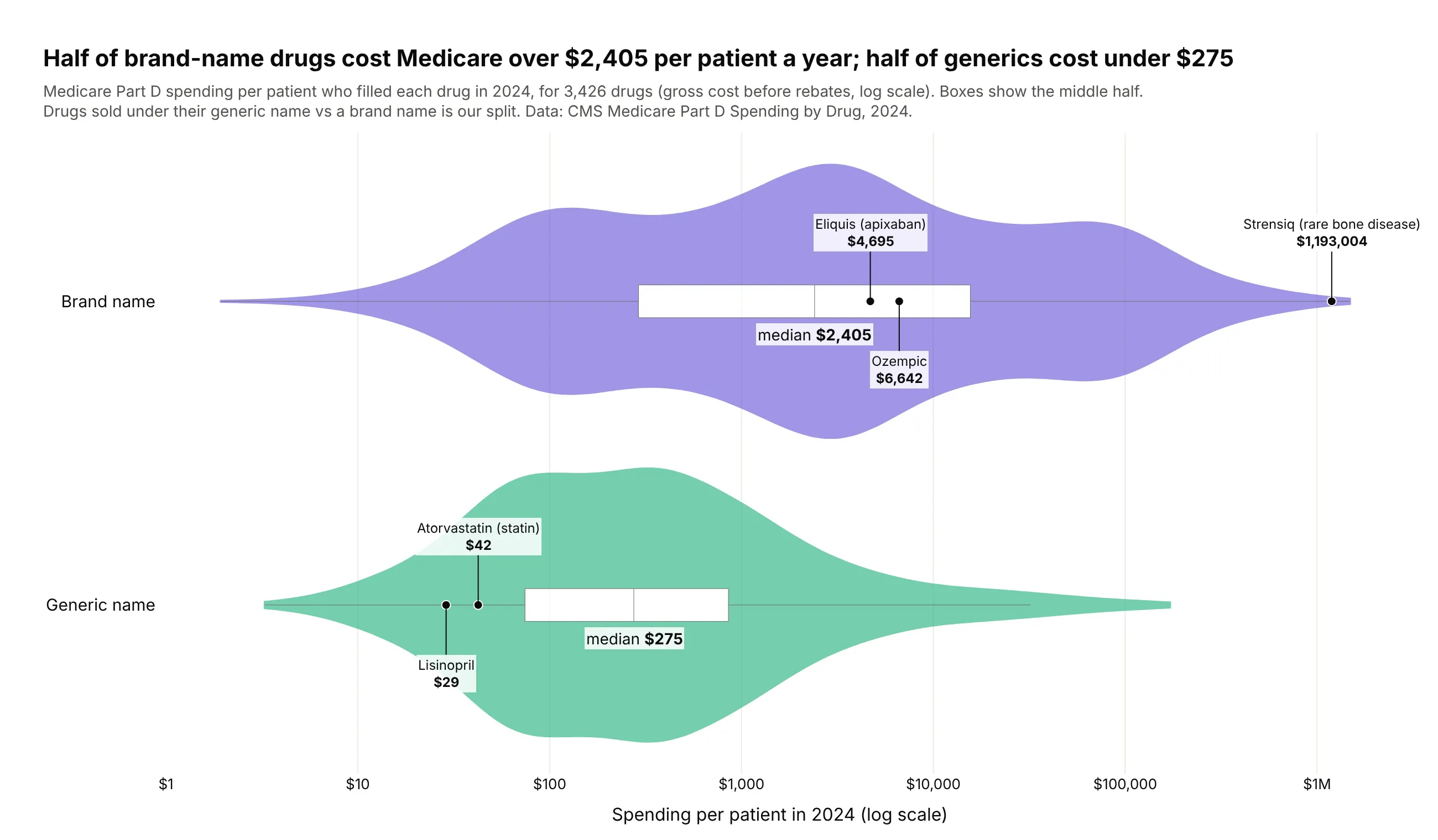
Half of brand-name drugs cost Medicare more than $2,405 per patient in 2024, while half of generics cost under $275. The brand violin reaches past $1 million a year for rare-disease drugs such as Strensiq ($1,193,004). Data: CMS Medicare Part D Spending by Drug, 2024 (brand/generic split is ours).

Tip: mark well-known items as labeled dots on their violin, so readers can place the distribution against drugs they know.

Get the data from CMS Medicare Part D Spending by Drug, 2024 (data.cms.gov) and shape it into a table
(columns: brand, generic, kind [Brand name / Generic name], spending_mn, beneficiaries, cost_per_bene),
using the "Overall" rows and drugs with 11+ beneficiaries.

Build two horizontal plotly violins of log10(cost_per_bene) by kind, inner box, ticks labeled $1 to $1M.
Mark Eliquis, Ozempic, Strensiq, atorvastatin and lisinopril as labeled dots. Title with both medians.

5. Life expectancy in every census tract, by state

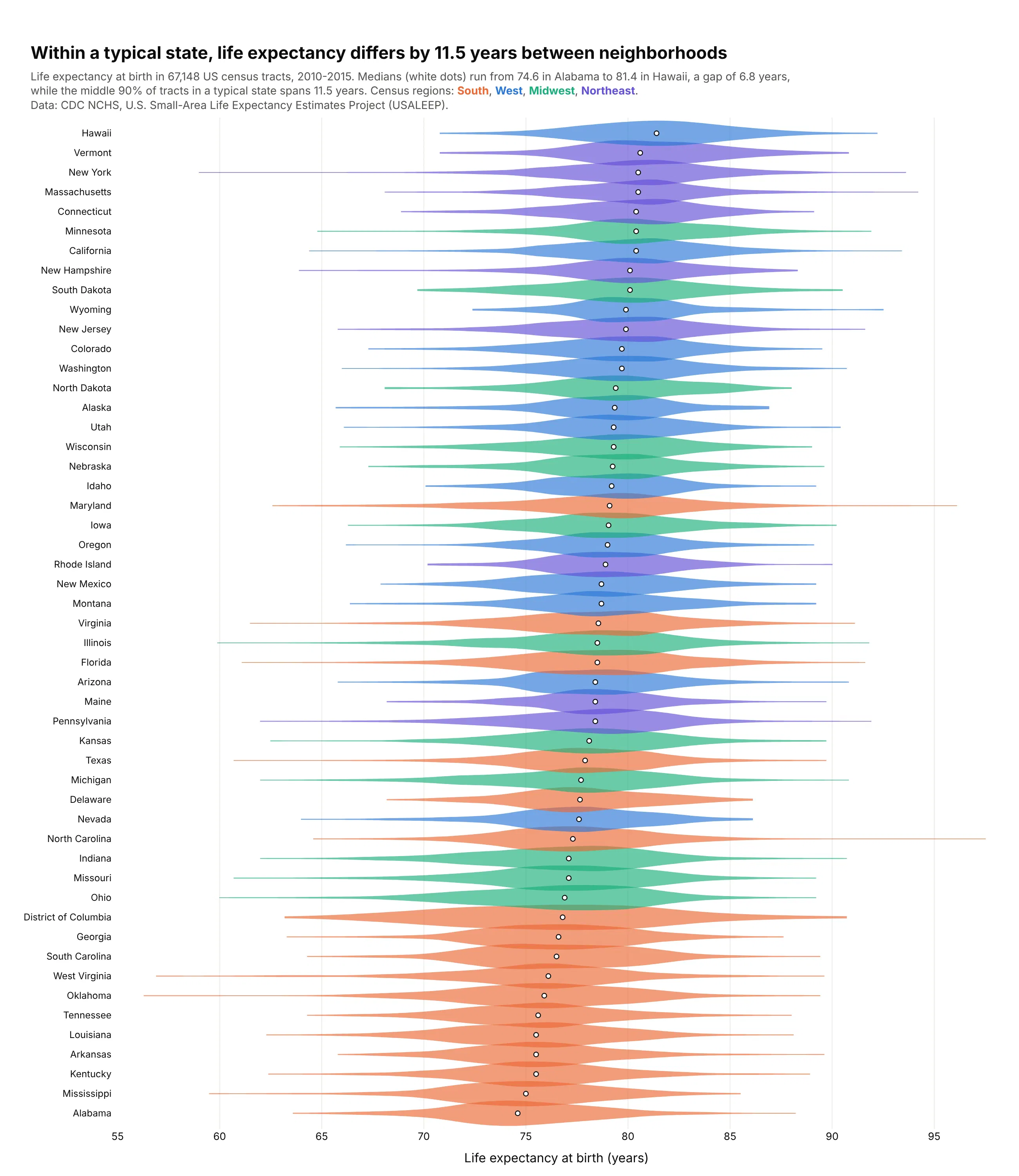
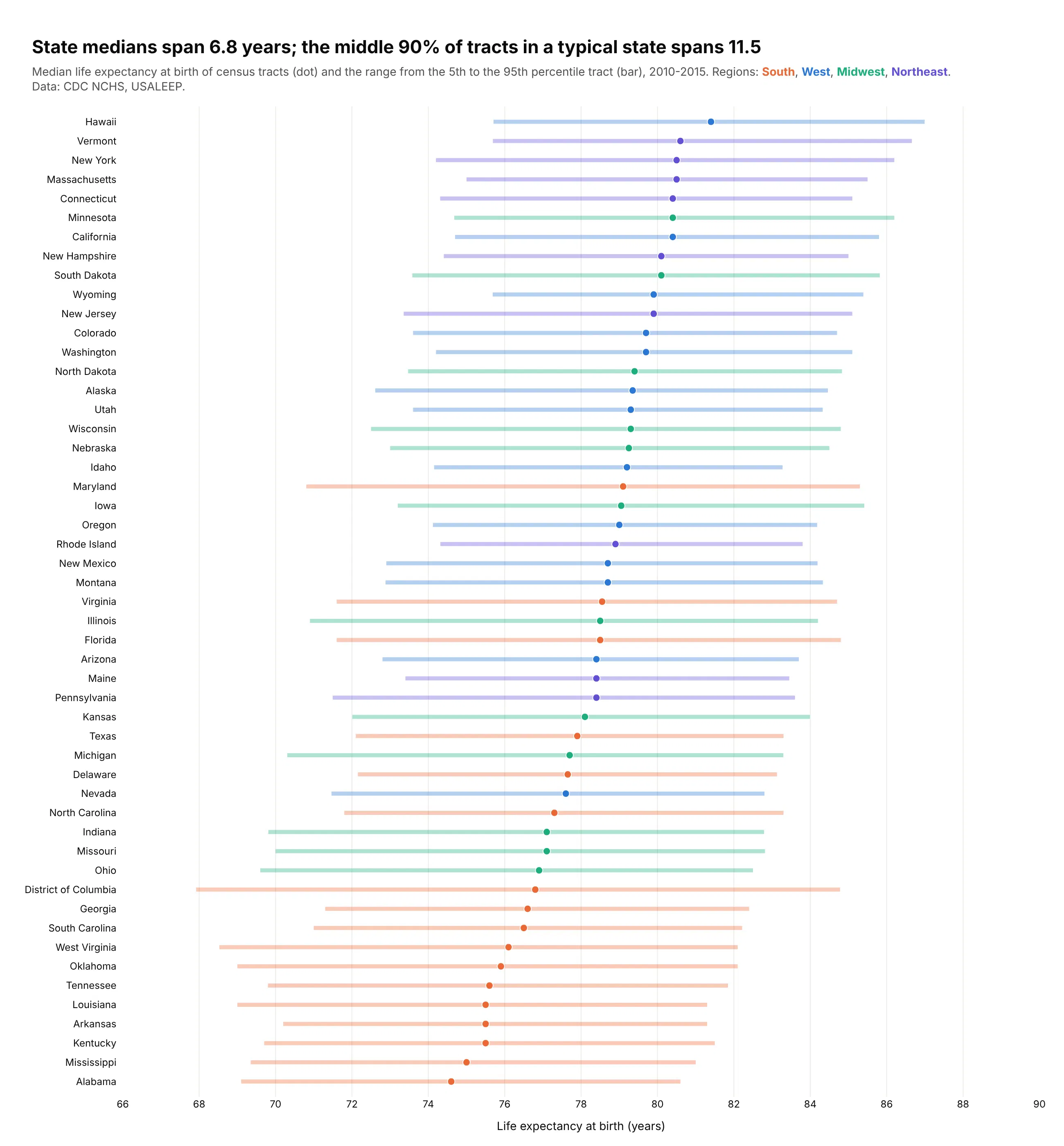
51 thin horizontal violins of life expectancy in 67,148 census tracts, one per state and DC, sorted by median and colored by census region. Medians run from 74.6 in Alabama to 81.4 in Hawaii, and the middle 90% of tracts in a typical state spans 11.5 years

State medians run from 74.6 years in Alabama to 81.4 in Hawaii, a 6.8-year gap. Inside a typical state, the middle 90% of neighborhoods spans 11.5 years, so where you live within a state matters more than which state. Data: CDC NCHS USALEEP, 2010-2015.

Tip: for 51 groups, use thin violins with only a median dot and a tall figure, and put the region colors in the subtitle instead of a legend.

Get the data from the CDC NCHS U.S. Small-Area Life Expectancy Estimates Project (USALEEP, US_A.CSV)
and shape it into a table (columns: tract, state, state_name, region, life_exp).

Build 51 horizontal plotly violins of life_exp, one per state, sorted by median, colored by census
region, width 1.25, no box, a white median dot, figure 1,500 px tall. Title with the typical
5th-95th percentile spread inside a state; subtitle with the range of state medians.

Another way to see it: a dot-and-range chart gives each state's median and 5th-95th percentile exactly, but loses the shape inside the range.

Each state's median tract life expectancy as a dot with a bar from the 5th to the 95th percentile tract, sorted, from Alabama (74.6) to Hawaii (81.4), with DC's bar the widest

6. Daily moves in the 10-year Treasury yield, by decade

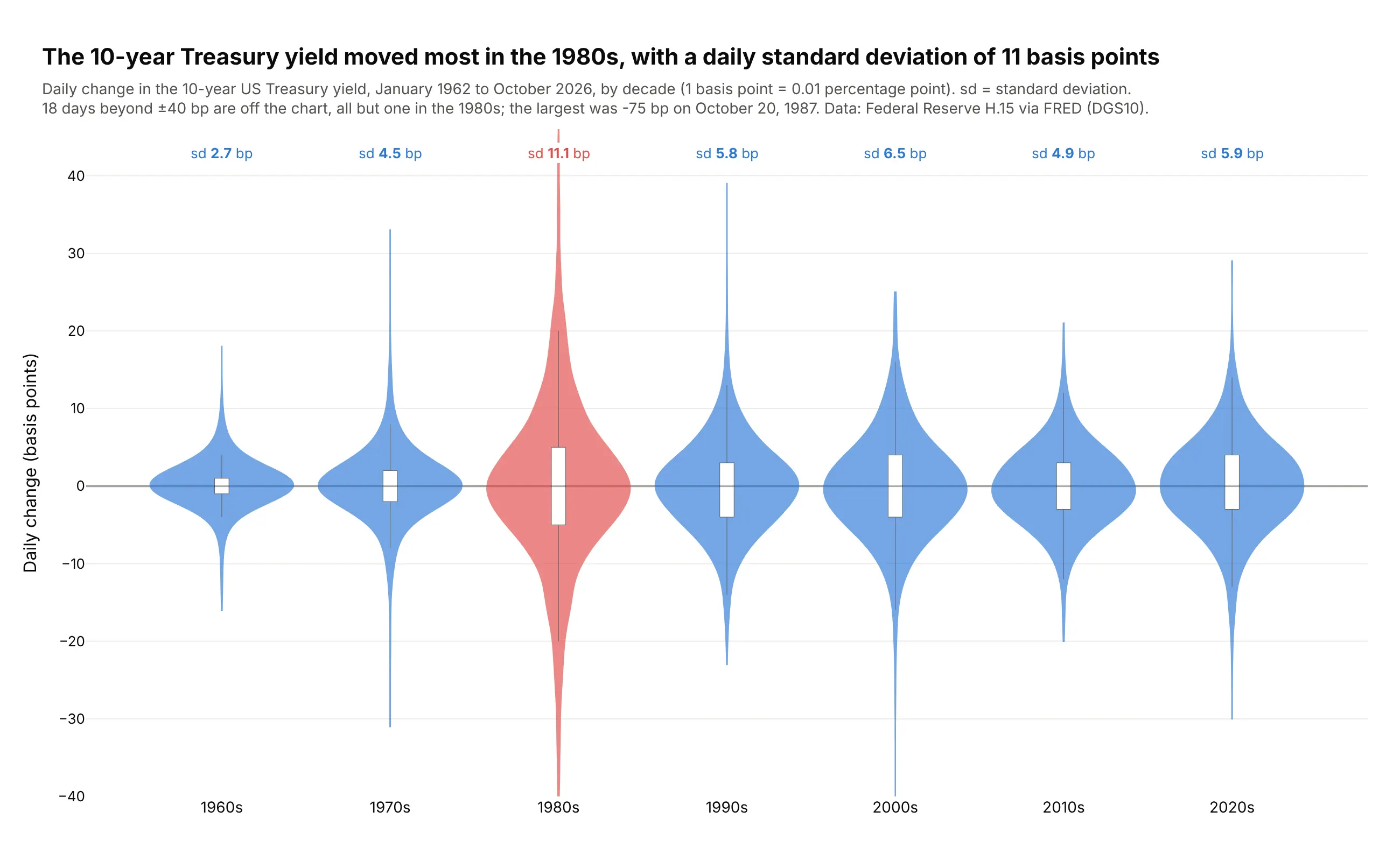
Violins of daily changes in the 10-year Treasury yield by decade from the 1960s to the 2020s, with the 1980s in red and a standard deviation of 11.1 basis points, against 2.7 in the 1960s

The 10-year yield moved most in the 1980s, with a daily standard deviation of 11.1 basis points, four times the 1960s (2.7). 17 of the 18 days beyond ±40 bp were in the 1980s. Data: Federal Reserve H.15 via FRED (DGS10), 1962-2026.

Tip: older yields are rounded to whole basis points, so set bandwidth=2; the default draws a comb of spikes for the 1960s.

Get the data from FRED series DGS10, the 10-year Treasury constant maturity yield (Federal Reserve H.15),
and shape it into a table (columns: date, decade, yield_pct, change_bp).

Build plotly violins of change_bp by decade with bandwidth=2, inner box, the 1980s in red. Print each
decade's standard deviation above it, clip at ±40 bp and name the largest day off the chart.

7. Central Park's nights, a century apart

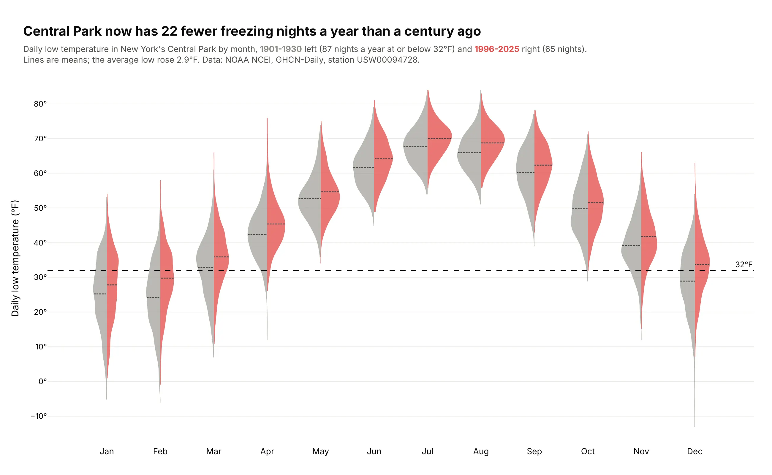
Split violins of daily low temperatures in Central Park by month, 1901-1930 in gray on the left and 1996-2025 in red on the right, with a dashed line at 32°F. Freezing nights fell from 87 to 65 a year

Central Park now has 22 fewer freezing nights a year than in 1901-1930 (65 vs 87), and the average low rose 2.9°F. Every month's violin moved up. Data: NOAA NCEI GHCN-Daily, station USW00094728.

Tip: split by period with the old one in gray and the recent one in a color, so color means "now".

Get the data from NOAA NCEI GHCN-Daily for station USW00094728 (NY City Central Park) and shape it into
a table (columns: date, year, month, period [1901-1930 / 1996-2025], tmax_f, tmin_f).

Build plotly split violins of tmin_f by month: 1901-1930 gray side="negative", 1996-2025 red
side="positive", mean lines, bandwidth 2, dashed line at 32°F. Title with the change in freezing
nights per year.

8. How deep large earthquakes start

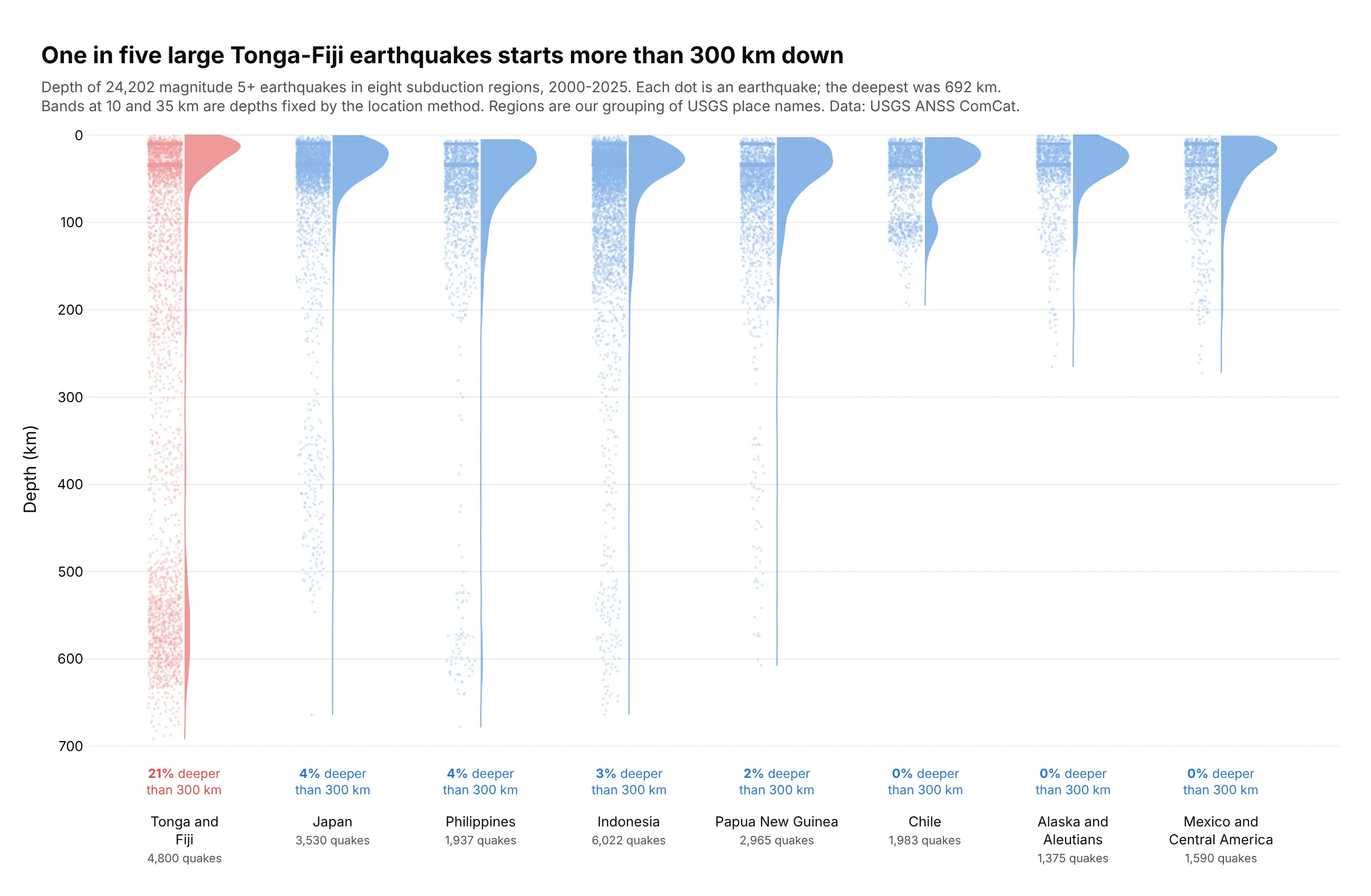
Half violins with jittered points of the depth of 24,202 magnitude 5+ earthquakes in eight regions, depth increasing downward. Tonga and Fiji in red have a second cluster 500-700 km down, and 21% of its earthquakes are deeper than 300 km

One in five large Tonga-Fiji earthquakes (20.7%) starts more than 300 km down, where the Pacific plate sinks into the mantle, and no other region tops 4.2%. The deepest was 692 km. Data: USGS ANSS ComCat, magnitude 5+, 2000-2025 (regions are ours).

Tip: reverse the y axis so depth goes down the page, and draw every event with points="all" next to a half violin.

Get the data from the USGS earthquake catalog (earthquake.usgs.gov/fdsnws/event/1/query), magnitude 5+,
2000-2025, and shape it into a table (columns: time, latitude, longitude, depth_km, mag, place, region)
with regions grouped from the place names.

Build plotly half violins (side="positive") of depth_km by region with points="all", jitter 0.3,
small transparent markers, y axis reversed. Highlight Tonga and Fiji and print each region's share
deeper than 300 km.

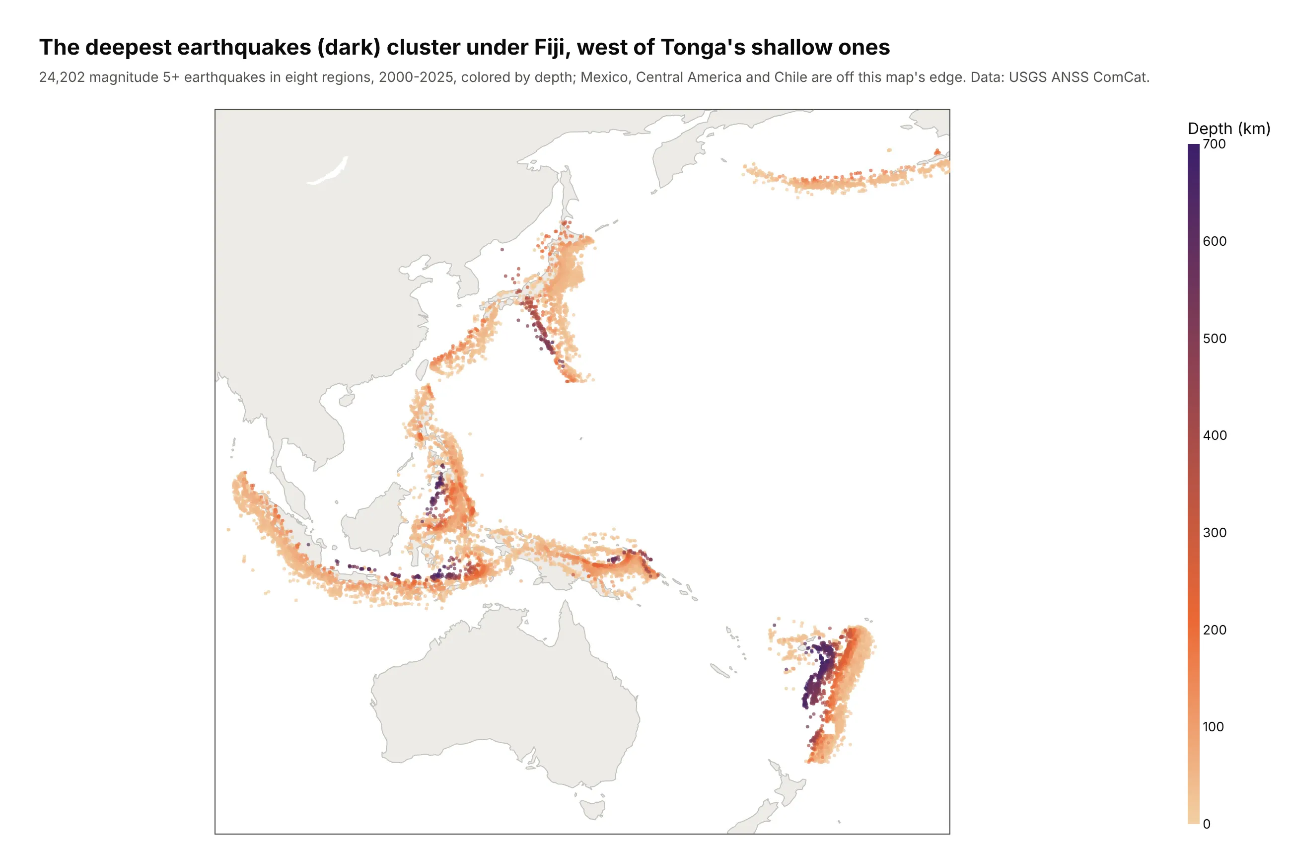
Another way to see it: a map shows where the deep events are, under Fiji to the west of Tonga's shallow ones, but not how many sit at each depth.

Map of the western Pacific with magnitude 5+ earthquakes colored by depth; the darkest, deepest events cluster under Fiji, west of the shallow ones along Tonga

9. Every MLB pitch in June 2025

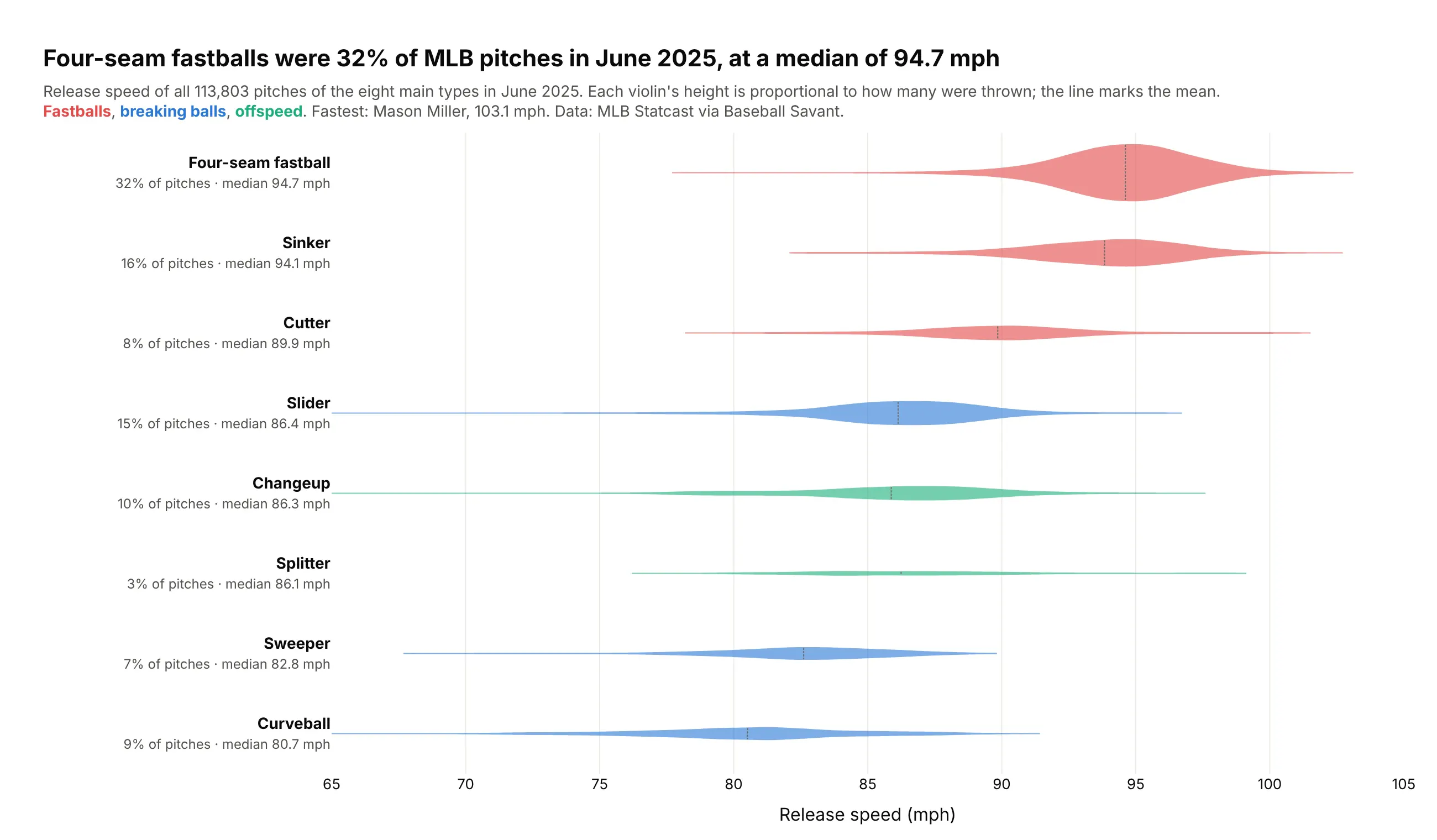
Horizontal violins of release speed for 113,803 MLB pitches in June 2025 by pitch type, with heights proportional to how often each is thrown: four-seam fastballs (32%, median 94.7 mph) dominate, splitters (3%) are a thin line

Four-seam fastballs were 32% of MLB pitches in June 2025, at a median of 94.7 mph. Splitters were 3%, but Jhoan Duran threw 45 of them at 97 mph or more, the bump at the right of that violin. Data: MLB Statcast via Baseball Savant.

Tip: scalemode="count" with one shared scalegroup makes each violin's size follow how often the pitch is thrown.

Get the data from Baseball Savant Statcast search CSV exports (baseballsavant.mlb.com/statcast_search),
regular-season pitches from 2025-06-01 to 2025-06-30, one request per day, and shape it into a table
(columns: pitcher_name, p_throws, pitch_type, release_speed).

Build horizontal plotly violins of release_speed for the eight main pitch types sorted by median,
scalemode="count", scalegroup="all", no width set, mean line, colored by family (fastballs,
breaking balls, offspeed). Labels with share of pitches and median.

10. How long New York takes to close a 311 request

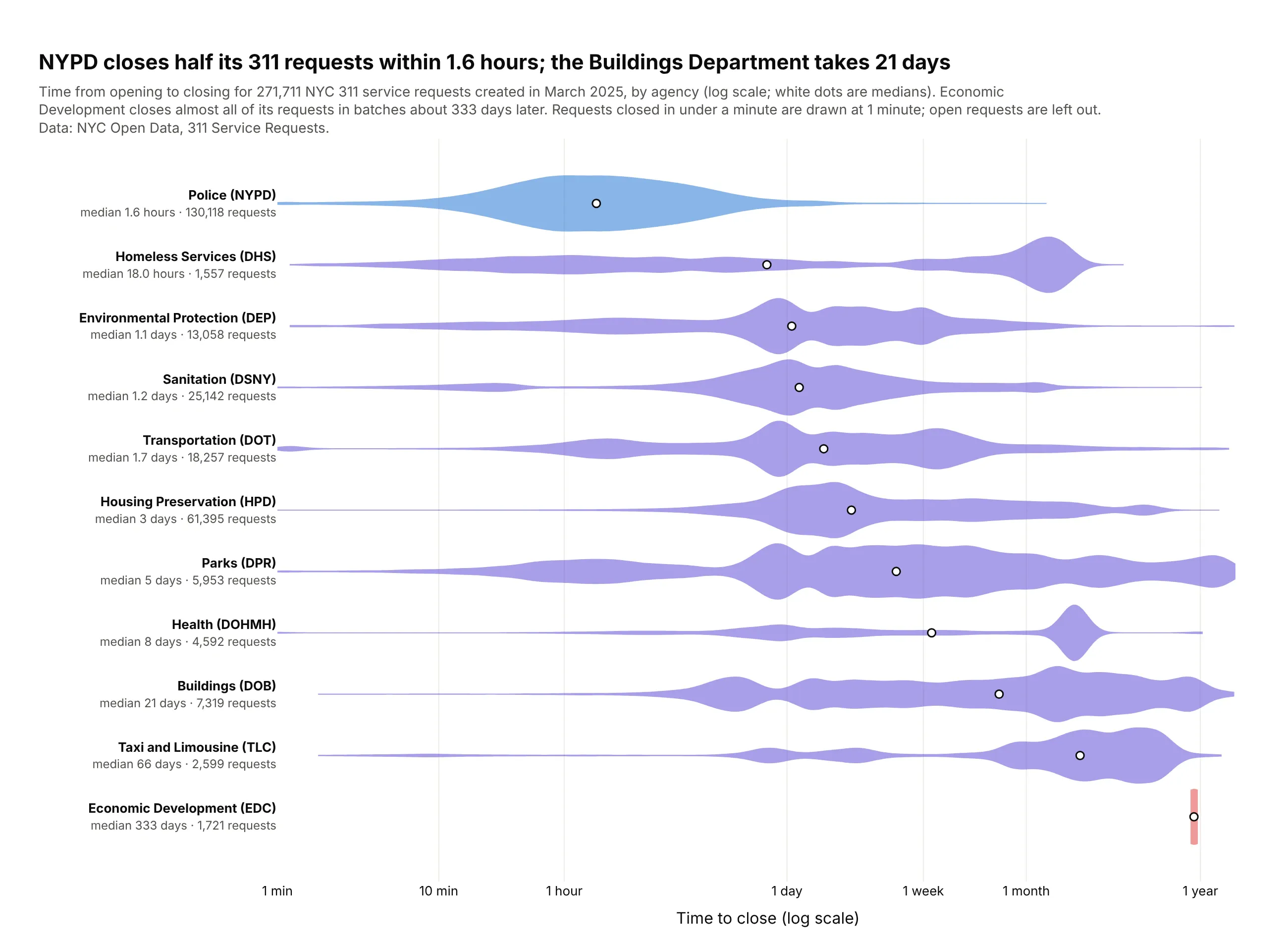
Horizontal violins of time to close 271,711 NYC 311 requests created in March 2025 by agency on a log scale from 1 minute to 1 year. NYPD's median is 1.6 hours, Buildings 21 days, and Economic Development closes nearly all its requests about 333 days later

NYPD closes half its 311 requests within 1.6 hours, while the Buildings Department takes 21 days. Several agencies have two or three humps (same day, a few days, months later), which a median alone would hide. Data: NYC Open Data, 311 requests created in March 2025.

Tip: label a log10 axis in plain time units (1 hour, 1 day, 1 week, 1 month, 1 year).

Get the data from NYC Open Data, 311 Service Requests (data.cityofnewyork.us, dataset erm2-nwe9),
requests created in March 2025, and shape it into a table (columns: agency, hours_to_close), dropping
open requests and zero or negative durations.

Build horizontal plotly violins of log10(hours_to_close) by agency sorted by median, bandwidth 0.08,
a white median dot, ticks labeled 1 min, 1 hour, 1 day, 1 week, 1 month, 1 year.
Title with the NYPD and Buildings medians.

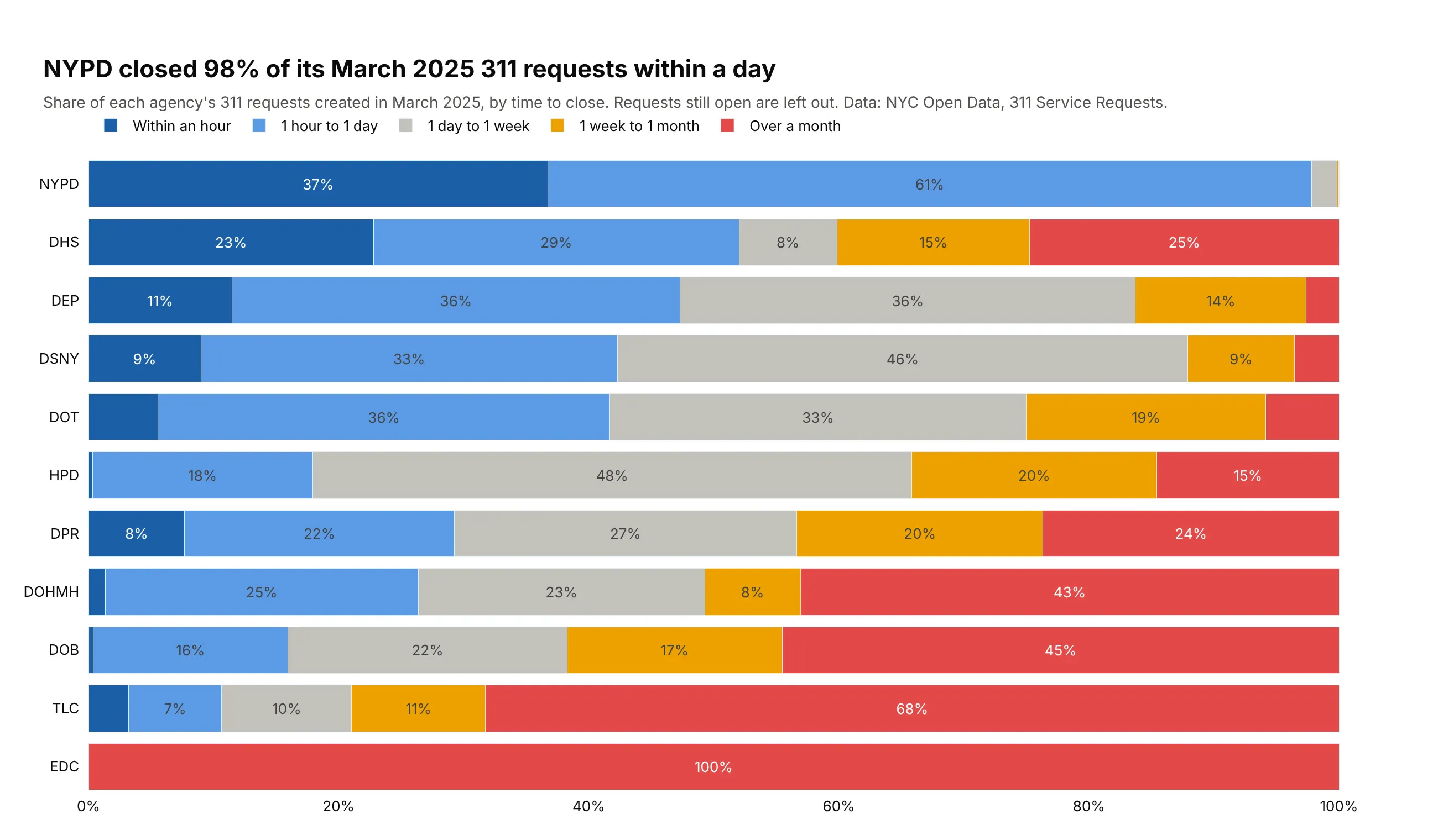
Another way to see it: stacked bars of time buckets give exact shares, such as 98% of NYPD requests closed within a day, but lose the shape inside each bucket.