
Chris Parmer
October 24, 2026
Ridgeline Plots - A Complete Guide
TL;DR
- A ridgeline plot stacks one smoothed distribution per group on a shared x axis, each overlapping the row above, so a dozen or more distributions fit in one chart.
- Ridgeline plots are also known as joyplots and ridge plots, and are similar to violin plots and histograms.
- Use one when the groups have a natural order (hours, months, years) or can be sorted by a statistic, and the question is how the shape shifts from row to row.
- Use violins or box plots instead for two or three groups or when exact quartiles matter, and a heatmap for hundreds of rows.
- You can make a ridgeline plot with Plotly from half violins (go.Violin with side="positive") or from filled go.Scatter curves of a density computed in numpy, and any coding agent can build one in a minute.
What is a ridgeline plot?
Ridgeline plots look like this:
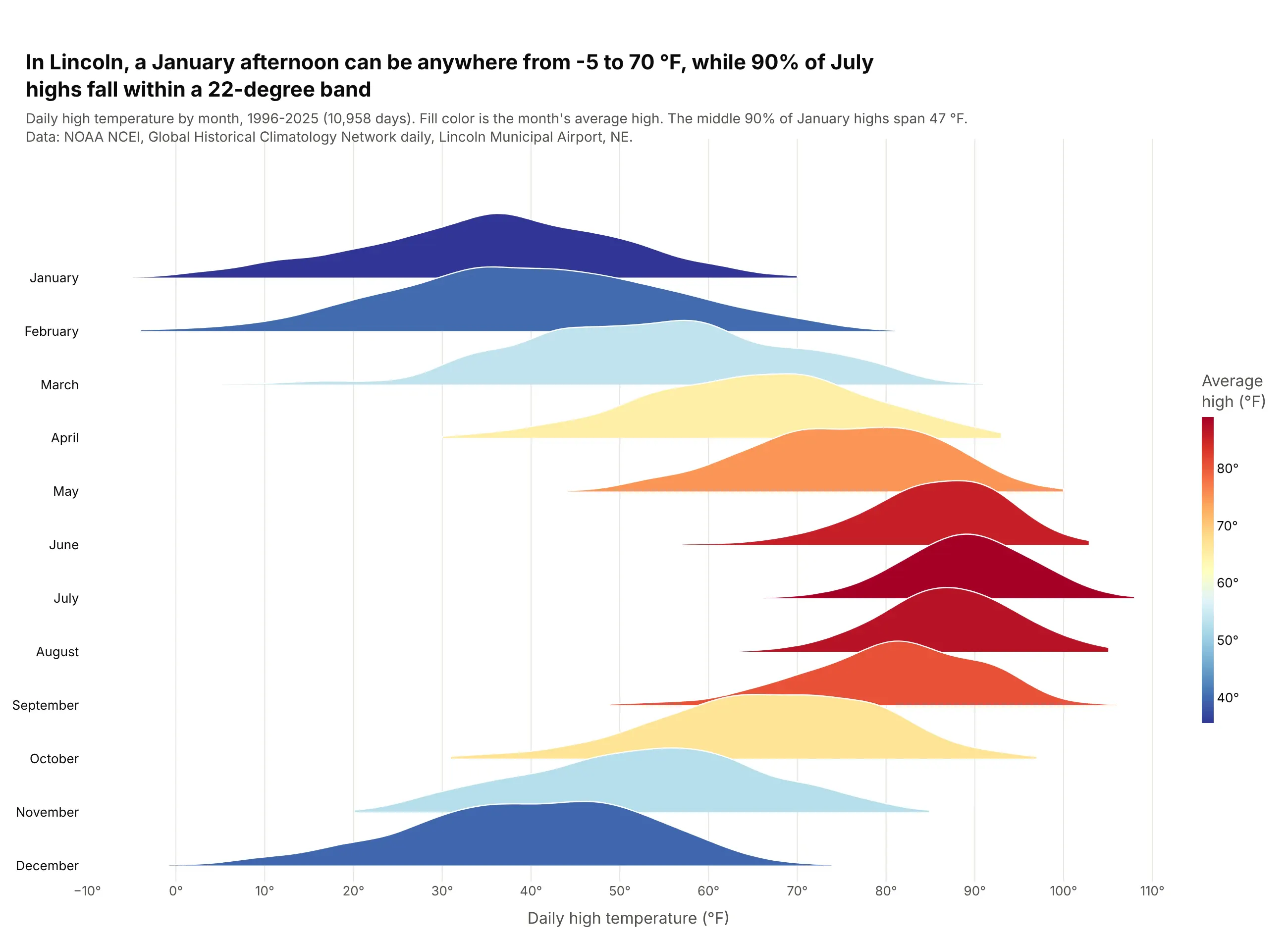
Data: NOAA NCEI, GHCN-Daily, Lincoln Municipal Airport, NE (USW00014939), 1996-2025.
How do you read a ridgeline plot? In the example above, notice these things:
- Each ridge is one month of daily highs in Lincoln, Nebraska, drawn as a density curve, which is a smoothed histogram. The taller the ridge at a temperature, the more days had that high.
- All the rows share one x axis, so you can follow the peak as it moves right from January to July and back left by December.
- The width of a ridge shows how much the weather varies in that month. The winter ridges are wide and the summer ridges narrow, so 90% of July highs fall within a 22-degree band while January's middle 90% spans more than twice that.
- The fill color repeats the month's average high on a blue-to-red scale, which makes the summer months read as one red block in the middle of the chart.
- Each ridge rises into the row above and covers part of it, and there is no scale for height. Compare the shapes and positions of the ridges, and leave exact day counts to a hover or a table.
It's often used for charts like these:
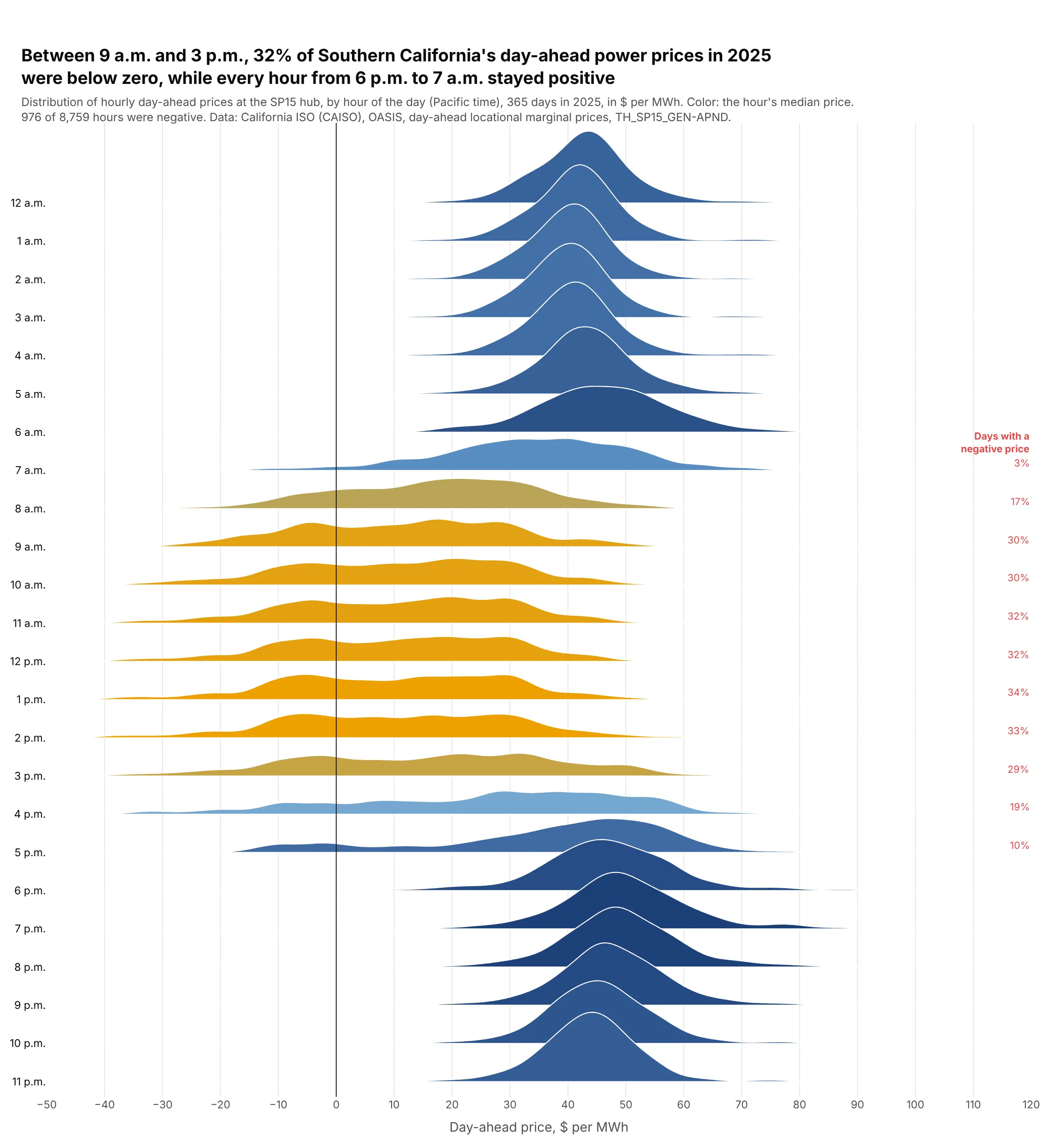
Prices by hour of the day. At the SP15 hub in Southern California, 32% of day-ahead power prices from 9 a.m. to 3 p.m. in 2025 were negative, when solar floods the grid, while night prices sat in a tight band around $40-50 per MWh. Data: California ISO, OASIS day-ahead prices, TH_SP15_GEN-APND, 2025.
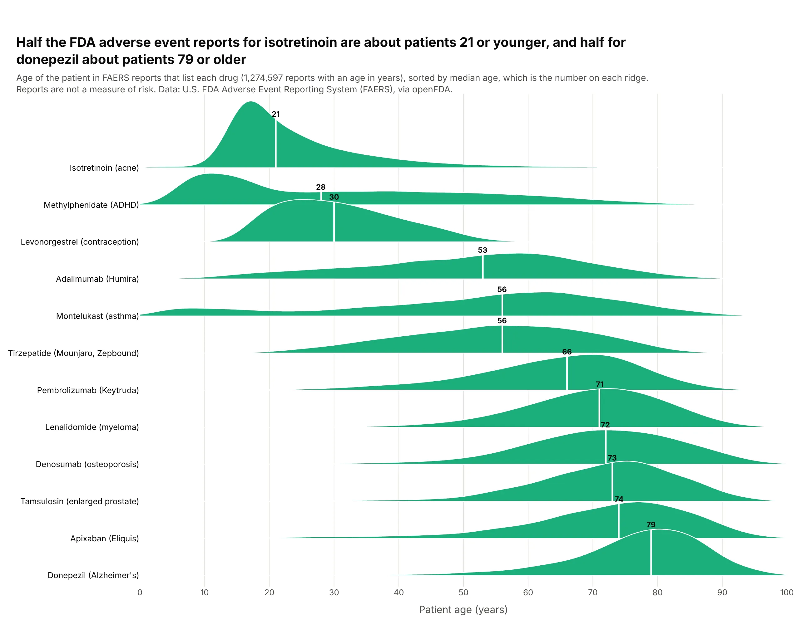
Groups sorted by their median. Sorted by median patient age in FDA adverse event reports, 12 drugs read as a lifespan, from isotretinoin (21) to donepezil (79), and the shapes show what medians can't, like montelukast's second bump of children. Data: FDA FAERS via openFDA, 1,274,597 reports with an age in years.
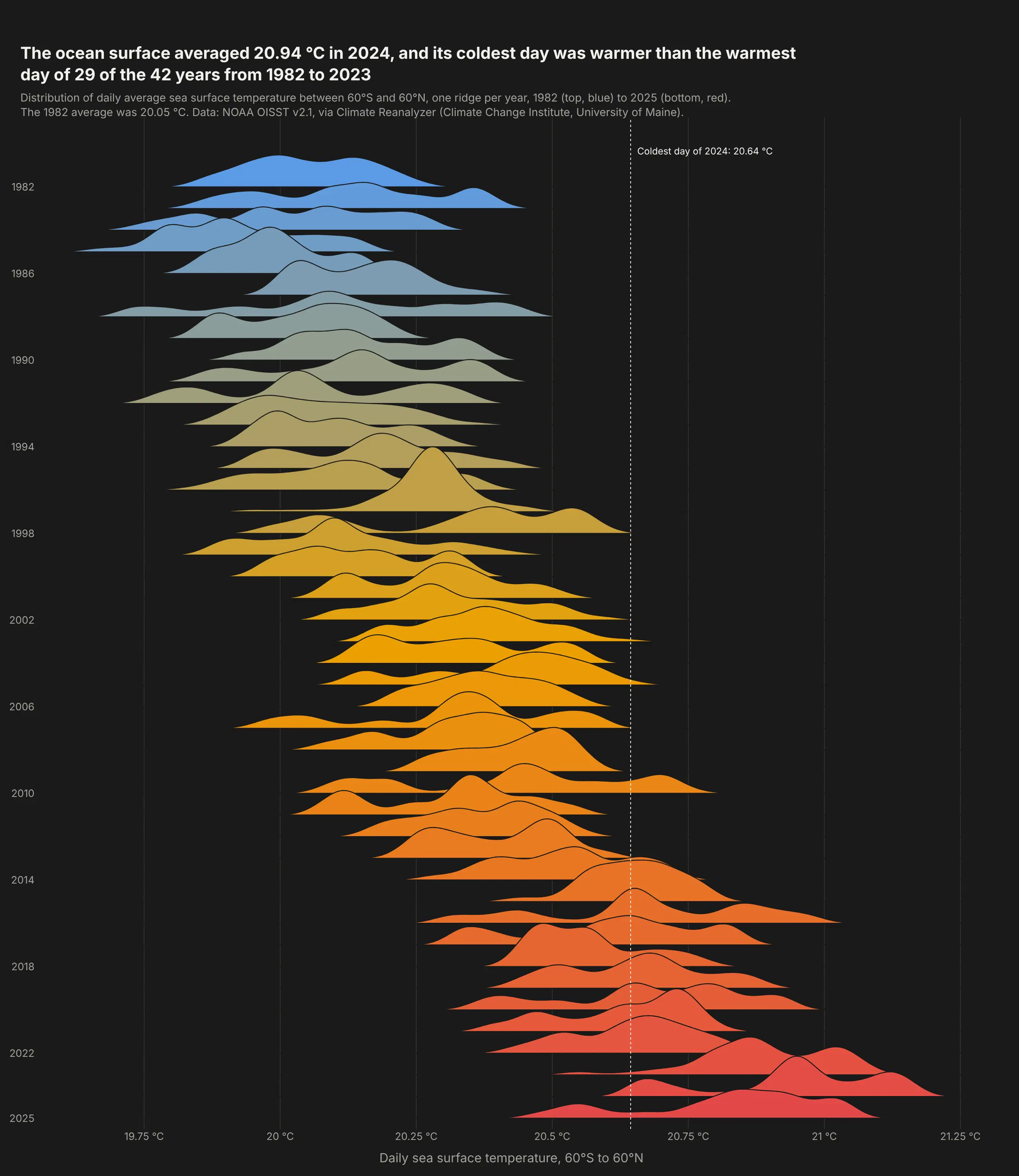
A long record, one row per year. The coldest day of 2024 on the ocean surface between 60°S and 60°N was warmer than the warmest day of 29 of the 42 years from 1982 to 2023. Data: NOAA OISST v2.1, via Climate Reanalyzer (University of Maine).
A short history
The look comes from radio astronomy. In his 1970 Cornell PhD thesis, Harold D. Craft Jr. plotted successive pulses of CP 1919, the first known pulsar (Hewish et al., 1968, Nature), as stacked lines, and Peter Saville put the plot on the cover of Joy Division's Unknown Pleasures in 1979 (Christiansen, Scientific American, 2015). Here it is redrawn with Plotly from approximate values read off Craft's figure:
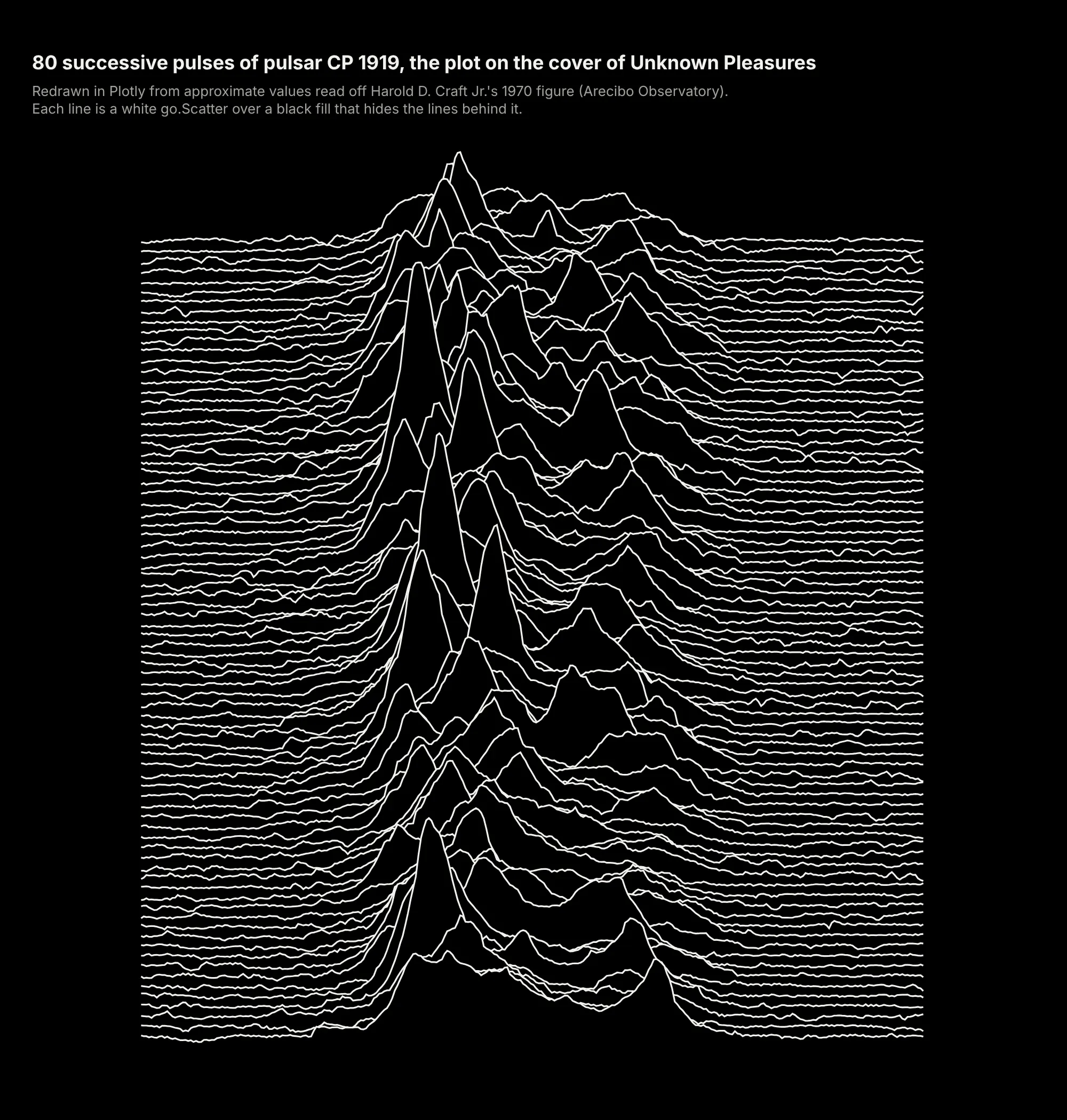
Jenny Bryan named the chart a "joyplot" in April 2017, after the album, and Claus Wilke's R package ggjoy made it popular. Wilke renamed it the ridgeline plot that September because the band's name comes from Nazi concentration camps (Wilke, 2017).
Alternatives to a ridgeline plot
Here's the same nine years of bank profitability drawn six ways. Some are better for the question, some worse, some just different:
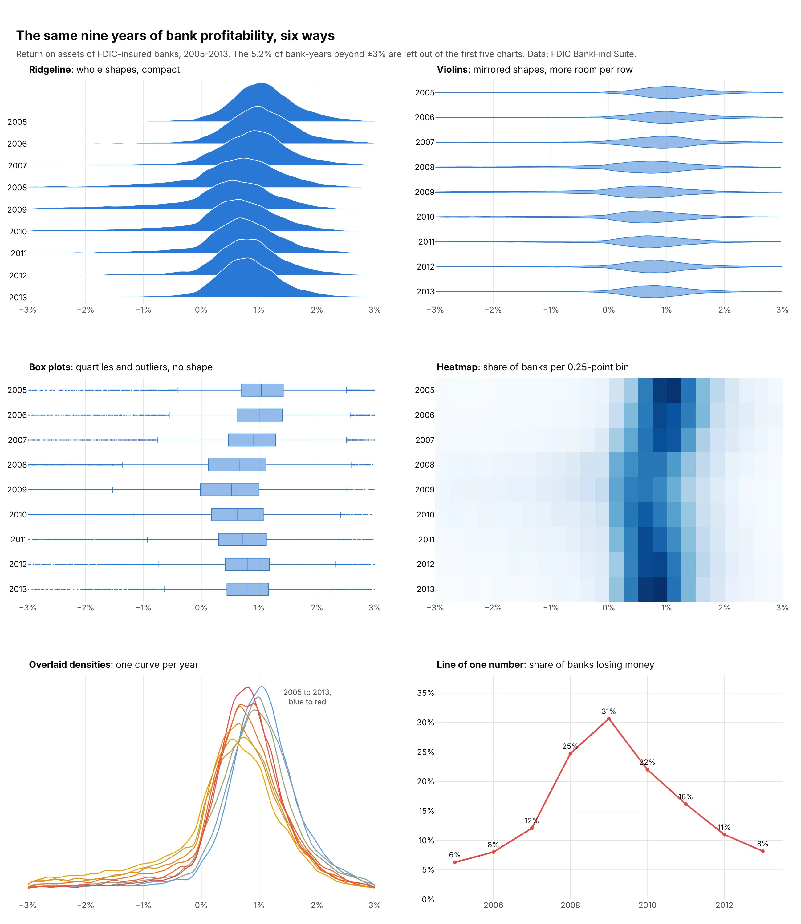
- Violin plot (works too, for a few groups). A violin mirrors each shape and gives every row its own space, which reads well for up to about eight groups but gets thin past that. See our violin plot guide.
- Box plot (worse when the shape matters, better for exact quartiles). Box plots show the median, quartiles and outliers precisely, but hide two peaks or a swelling tail. See our box plot guide.
- Heatmap (better for hundreds of rows). Binned shares as color scale to hundreds of rows in the same space, but color is harder to read than height. See our heatmap guide.
- Overlaid densities or histograms (worse past three groups). On one baseline you can compare two or three shapes directly, but nine curves turn into a tangle. See our histogram guide.
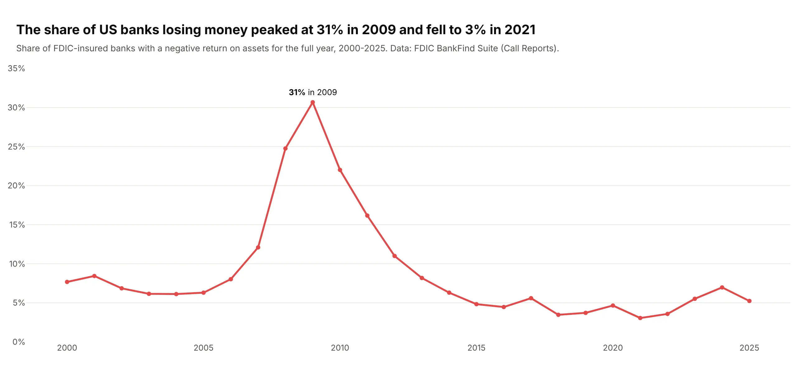
- Line of one statistic (better when one number is the story). The share of banks losing money, 8% in 2006 and 31% in 2009, reads exactly from a line, but the rest of each distribution disappears.
How to make a ridgeline plot
With AI
ChatGPT, Claude Code, GitHub Copilot, Cursor and other AI tools are excellent at writing Plotly code. Name Plotly in the prompt, and spell out the rows, the order, the overlap, the bandwidth and the checks you want:
Make a plotly ridgeline plot from readings.csv (columns: sensor_id, site, timestamp, value).- One row per site, sorted by median value (lowest at the top).- Compute a Gaussian kernel density per row in numpy on a 300-point gridwith ONE shared bandwidth; draw each ridge as a go.Scatter with fill="toself",lifted to its row's baseline. Overlap = 1.8 rows; heights on one shared scale.- Draw the top row first so each lower ridge sits in front; white 1.2 px outlines.- One color (#2a78d6); print each row's median and sample size at the right end.- Cut the grid at the data's min and max; no curve beyond the data.- A title that states the takeaway, source in a subtitle.- Check: print each row's sample size and warn if any row has fewer than 30 values.- Save it as ridgeline.html and as a PNG at 2x scale.
Keep the sample-size check in every ridgeline prompt, because a smooth curve on 12 values looks as confident as one on 12,000.
With Plotly Studio
Plotly Studio is a desktop app where you point an AI at a dataset and it builds charts and a Dash app around your questions. Ask for a ridgeline plot the same way:
Make a ridgeline plot of daily electricity prices with one row per hour of the day, midnight at the top. Use an overlap of about 2 rows, color each ridge by its median price and draw a line at zero. Add a dropdown to switch between years.
Make a ridgeline plot in Python or JavaScript
This is the code AI tools write under the hood. In Python, this helper computes a density per row in numpy and draws each one as a filled go.Scatter, lifted to its row and drawn back to front. It takes a shared or per-row bandwidth, weights for pre-counted data and an optional fill by each row's mean or median, and the figure stays small however many values go in:
import numpy as npimport pandas as pdimport plotly.colors as pcimport plotly.graph_objects as godef kde(values, grid, bandwidth=None, weights=None):v = np.asarray(values, float)w = np.ones_like(v) if weights is None else np.asarray(weights, float)w = w / w.sum()if bandwidth is None: # Silverman's rule, per rowsd = np.sqrt(np.sum(w * (v - np.sum(w * v)) ** 2))bandwidth = 0.9 * sd * (1 / np.sum(w ** 2)) ** -0.2z = (grid[:, None] - v[None, :]) / bandwidthreturn (np.exp(-0.5 * z ** 2) * w).sum(axis=1) / (bandwidth * np.sqrt(2 * np.pi))def make_ridgeline(df, x, row, order=None, weights=None, overlap=1.5, bandwidth=None,color="#2a78d6", fill_by=None, colorscale="RdBu_r", points=200):order = list(order if order is not None else df[row].drop_duplicates()) # top to bottomgrid = np.linspace(df[x].min(), df[x].max(), points)curves, stats = {}, {}for r in order:d = df[df[row] == r]w = d[weights] if weights else Nonecurves[r] = kde(d[x], grid, bandwidth, w)stats[r] = np.average(d[x], weights=w) if fill_by == "mean" else d[x].median()top = max(c.max() for c in curves.values())lo, hi = min(stats.values()), max(stats.values())fig, n = go.Figure(), len(order)for i, r in enumerate(order): # the top row is drawn first, so lower ridges sit in frontbase = n - 1 - iy = base + curves[r] / top * overlapfill = pc.sample_colorscale(colorscale, (stats[r] - lo) / (hi - lo or 1))[0] if fill_by else colorfig.add_trace(go.Scatter(x=np.r_[grid, grid[::-1]], y=np.r_[y, np.full(points, base)],fill="toself", fillcolor=fill, line=dict(color="white", width=1.2),mode="lines", name=str(r), hoveron="fills", showlegend=False))fig.update_layout(template="simple_white", yaxis=dict(tickvals=list(range(n)), ticktext=[str(r) for r in order][::-1],range=[-0.2, n - 1 + overlap + 0.1], showline=False, ticks=""))return figweather = pd.read_csv("https://raw.githubusercontent.com/plotly/datasets/master/2016-weather-data-seattle.csv")weather["month"] = pd.to_datetime(weather.Date).dt.strftime("%b")months = ["Jan", "Feb", "Mar", "Apr", "May", "Jun", "Jul", "Aug", "Sep", "Oct", "Nov", "Dec"]fig = make_ridgeline(weather, x="Max_TemperatureC", row="month", order=months, fill_by="mean", overlap=1.8)fig.show()
In JavaScript, plotly.js builds the same kind of chart from half violins: one violin trace per row with side: "positive" and a width above 1, so each ridge overlaps the row above. The browser computes the densities:
<div id="chart"></div><script src="https://cdn.plot.ly/plotly-4.1.1.min.js"></script><script>fetch("https://raw.githubusercontent.com/plotly/datasets/master/violin_data.csv").then((r) => r.text()).then((csv) => {const [head, ...lines] = csv.trim().split("\n").map((l) => l.split(","));const bill = head.indexOf("total_bill"), day = head.indexOf("day");const days = ["Thur", "Fri", "Sat", "Sun"]; // top row first, so lower ridges sit in frontPlotly.newPlot("chart", days.map((d) => ({type: "violin", orientation: "h", side: "positive", width: 2,x: lines.filter((l) => l[day] === d).map((l) => +l[bill]), y0: d, name: d,points: false, spanmode: "hard", line: {color: "white"}, fillcolor: "#2a78d6"})), {showlegend: false, violinmode: "overlay", violingap: 0,yaxis: {categoryorder: "array", categoryarray: [...days].reverse()}});});</script>
Half violins are the shortest way, and Python's go.Violin takes the same settings. For big data, compute the density in Python instead, because violins send every raw value to the browser (see the FAQ for timings).
Share it
Every Plotly chart has a Share chart button (the cloud icon in its toolbar) that uploads it to Plotly Cloud and gives you a link. Only you can see it until you change its visibility.
For a live app, put the chart in a Dash app and publish it with the Plotly Cloud CLI. Coding agents can run these commands for you:
pip install "dash[cloud]"plotly user loginplotly app publish
If your data has to stay in your own cloud or data center, publish to Dash Enterprise instead.
Dos and don'ts
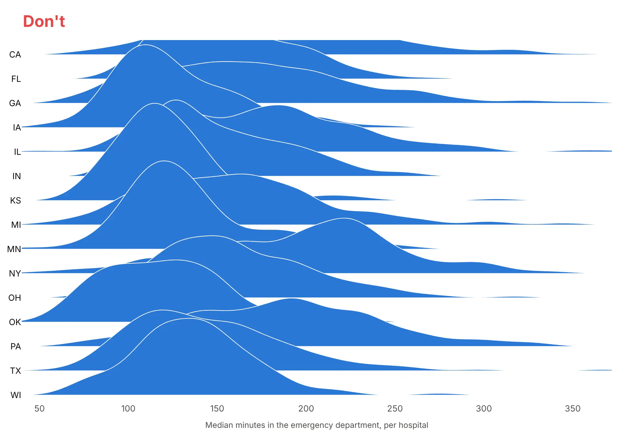
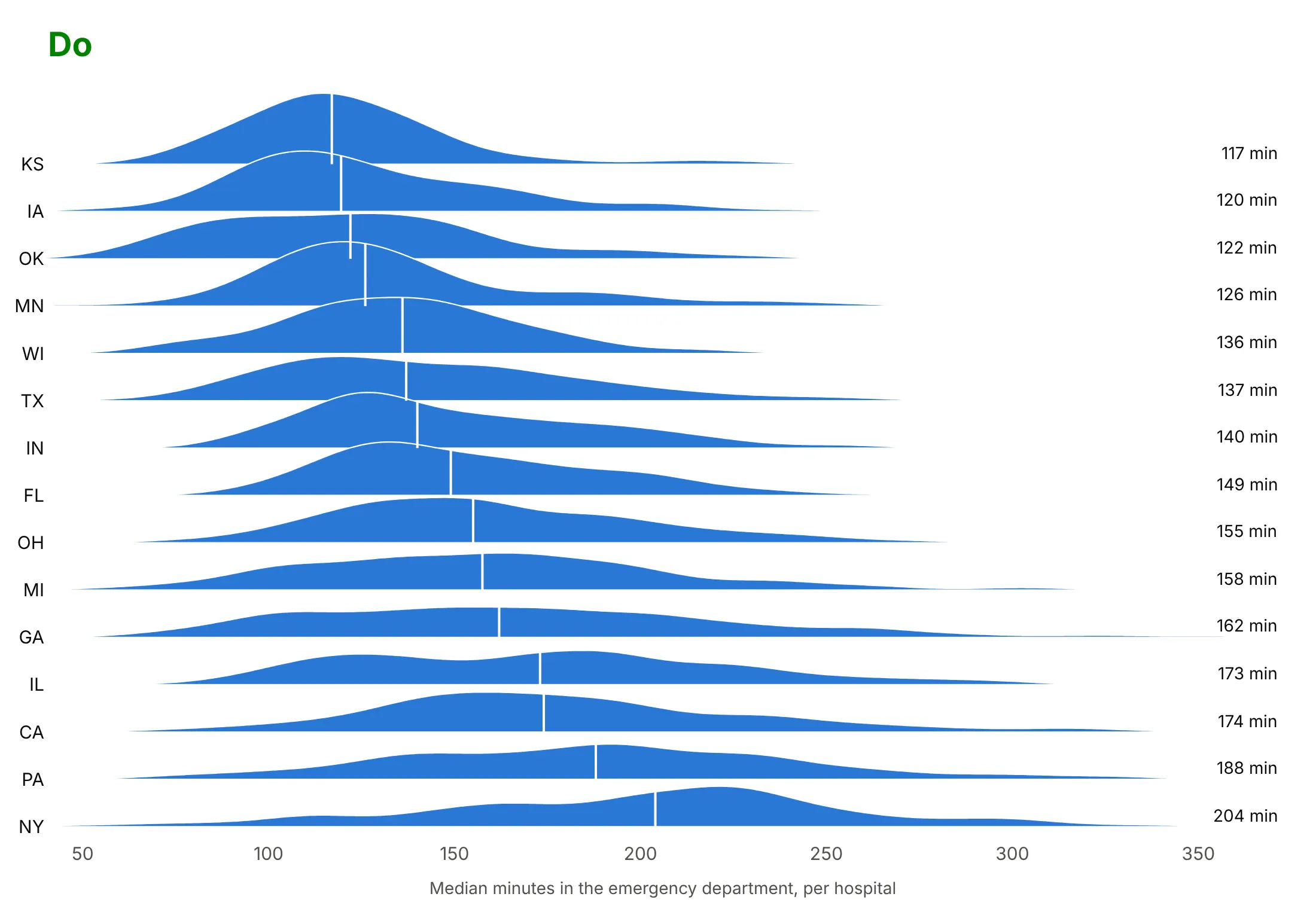
Most of the work in a ridgeline is ordering the rows, setting the overlap and deciding which number to print. Here is the same emergency department data for the 15 states with the most hospitals both ways, in the same blue.
Don't leave the rows in alphabetical order, set the overlap so high that tall ridges hide the rows behind them, clip the top ridge with the axis range, or leave every number off the chart:
Do sort the rows by the median, keep the overlap near 1.5 rows with room above the top ridge, and print the number that matters on each row. Here the medians run from 117 minutes in Kansas to 204 in New York:
Use color for one thing
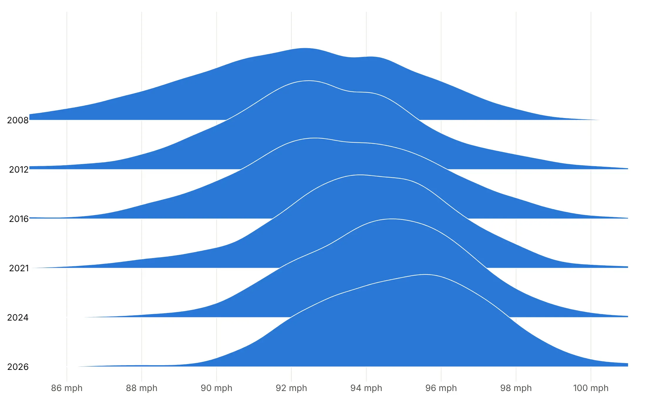
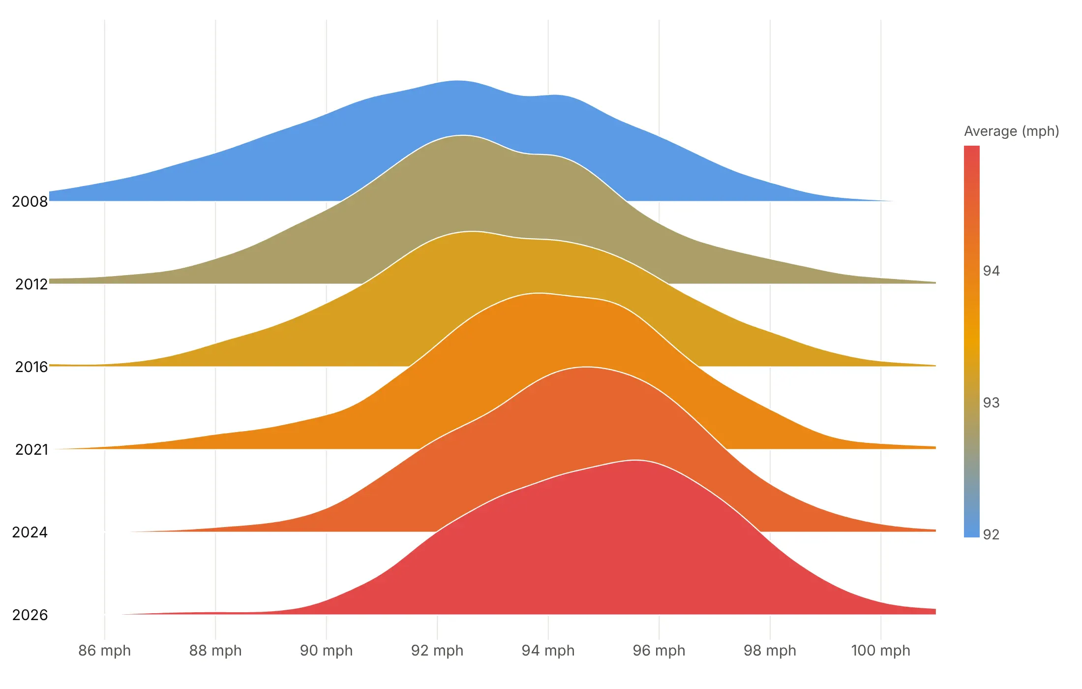
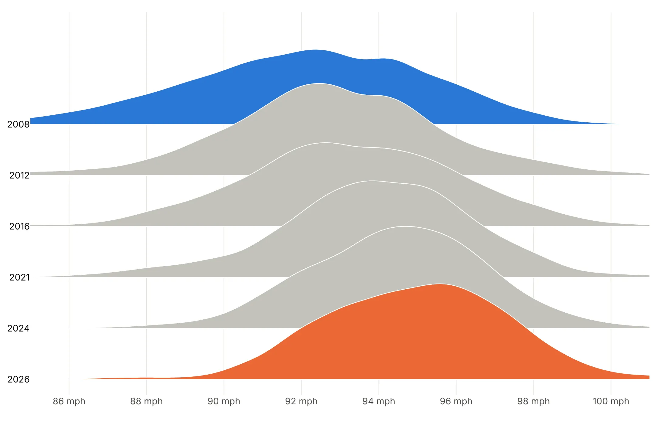
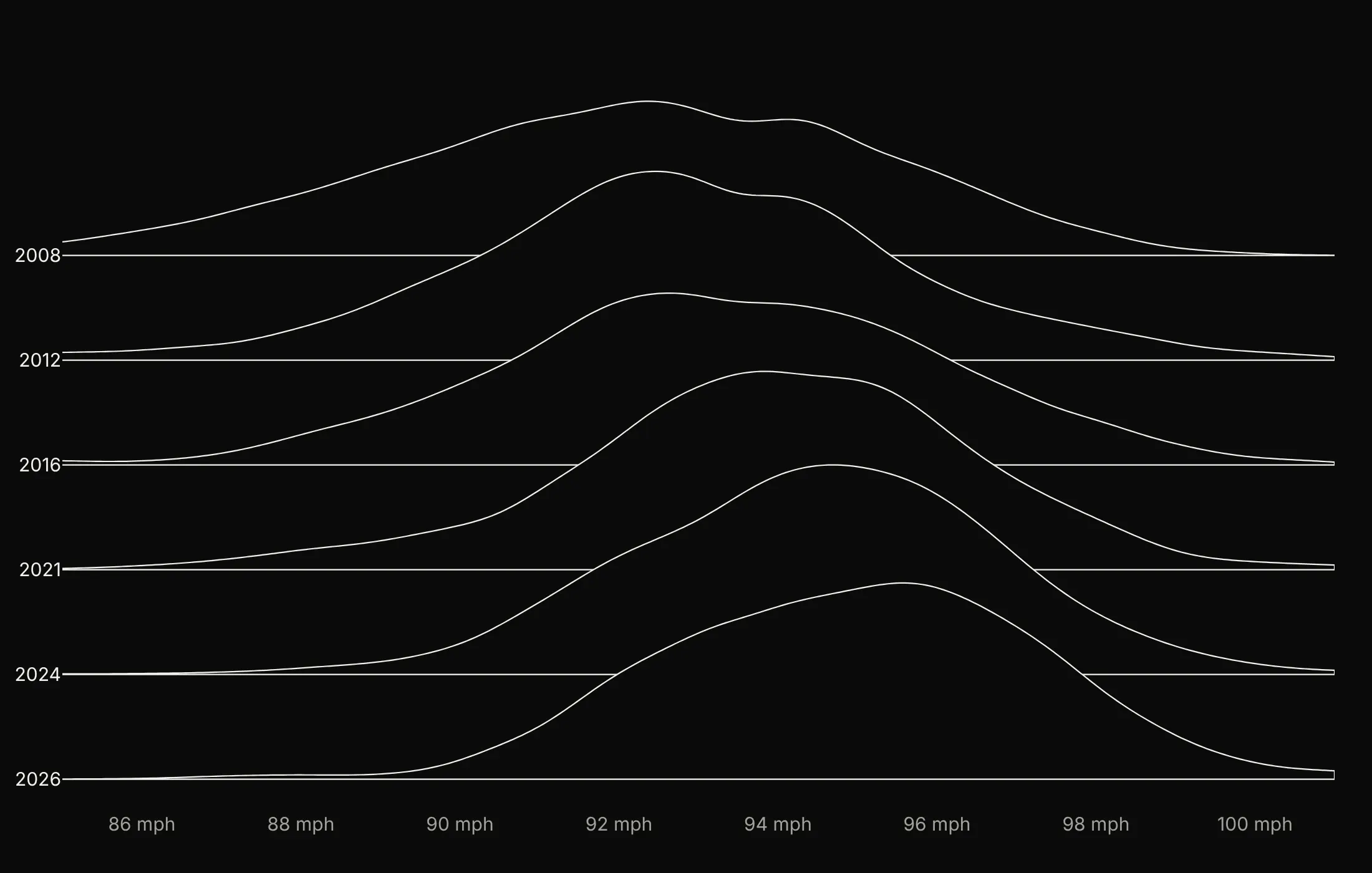
One color always works. When you want color to say something, pick one thing for it to say. Here are four options on the same MLB fastball speeds for six seasons.
One color. The safe default, because the rows are already labeled.
Color by a value. Each ridge is filled by the season's average speed, which went from 92.0 mph in 2008 to 95.0 mph in 2026.
Highlight the rows you compare. Gray everything except 2008 in blue and 2026 in orange, so the comparison reads first and the gray rows show the steady drift between them.
Outlines on black. White lines over a dark fill give the Unknown Pleasures look, which works for a cover image more than for reading values.
Checklist
Do
- Write a title that states the takeaway with a number, and put the source in a muted subtitle.
- Order rows by time or by the statistic that matters (a median, or a tail share such as flights over an hour late).
- Set the overlap, the height of the tallest ridge in rows, to about 1.5 to 2, and up to 3 for many rows of similar height.
- Draw the top row first with white outlines, so each lower ridge sits in front.
- Use one shared bandwidth when rows are compared, and print the sample size when rows differ in size.
- Use a log axis for prices, flows and salaries, with the density computed on the log values.
Don't
- Sort rows alphabetically, or set the overlap so high that tall ridges hide whole rows.
- Use a rainbow of colors that mean nothing for rows that are already labeled.
- Draw tails past the data: cut the curve at the data range (spanmode="hard" for violins).
- Smooth tiny samples without showing the raw points.
- Clip the top ridge: leave one overlap of room above the top row.
Options to customize
These are the options that matter most for building a ridgeline from go.Violin or from go.Scatter. The full references are in the Plotly violin plot and filled area documentation.
- go.Violin(orientation="h", side="positive"): horizontal half violins, one per y0, for the violin method.
- width: the height of each violin in rows; above 1 makes the rows overlap (2 to 3 is typical).
- bandwidth: the kernel bandwidth; set the same value on every trace for a shared bandwidth.
- spanmode="hard": stops the curve at the data's range, for bounded values such as ages.
- violinmode="overlay", violingap=0 (layout): let the rows overlap; always use them with violins.
- scalemode="count": makes each violin's size follow its sample size, when row sizes should show.
- go.Scatter(fill="toself"): fills a precomputed curve down to its baseline, for the numpy method.
- fillcolor, line.color: fill and outline, for one color, a highlight or a scale.
- fillgradient: a gradient fill along x or y, for color that follows the x value.
- line.simplify=False: keeps every outline point, for smooth curves in static images.
- hoveron="fills": hover over the whole ridge to show a row's median or count.
- Trace order: later traces draw on top, so add the top row first.
- yaxis.tickvals, ticktext, range: row labels and headroom for the numpy method; leave one overlap above the top row.
- xaxis.type="log": a log x axis, for prices, flows and salaries.
More ridgeline plot examples
Ten more ridgeline plots built from real public data, each with its source, the technique that makes it work and a prompt to rebuild it.
1. Henry Hub natural gas, 18 years of daily prices
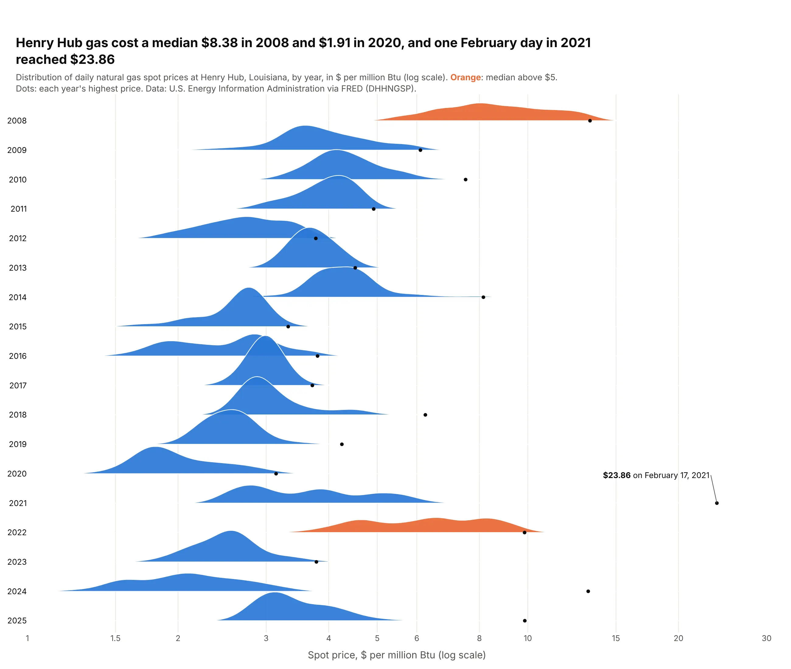
The median Henry Hub price was $8.38 per million Btu in 2008 and $1.91 in 2020, and only 2008 and 2022 had medians above $5. The dots show how far single days jump: on February 17, 2021, during the Texas freeze, gas reached $23.86. Data: U.S. EIA Henry Hub spot price via FRED (DHHNGSP), 2008-2025.
Tip: compute the density on log10(price) and draw it on a log axis, so $2 to $4 looks as big a move as $4 to $8.
Get the data from the U.S. Energy Information Administration's Henry Hub natural gas spot price series(daily, $ per million Btu; FRED series DHHNGSP) for 2008-2025 and shape it into a table(columns: date, year, price).Build a plotly ridgeline plot with one row per year, 2008 at the top.- Kernel density on log10(price) (bandwidth 0.03), drawn on a log x axis from $1 to $30.- Overlap 1.7; years with a median above $5 in orange, others in blue.- A small black dot at each year's highest price; annotate the overall maximum with its date.- Title with the highest and lowest yearly medians; cite EIA via FRED.
2. Every new mortgage in Colorado, 2018-2025
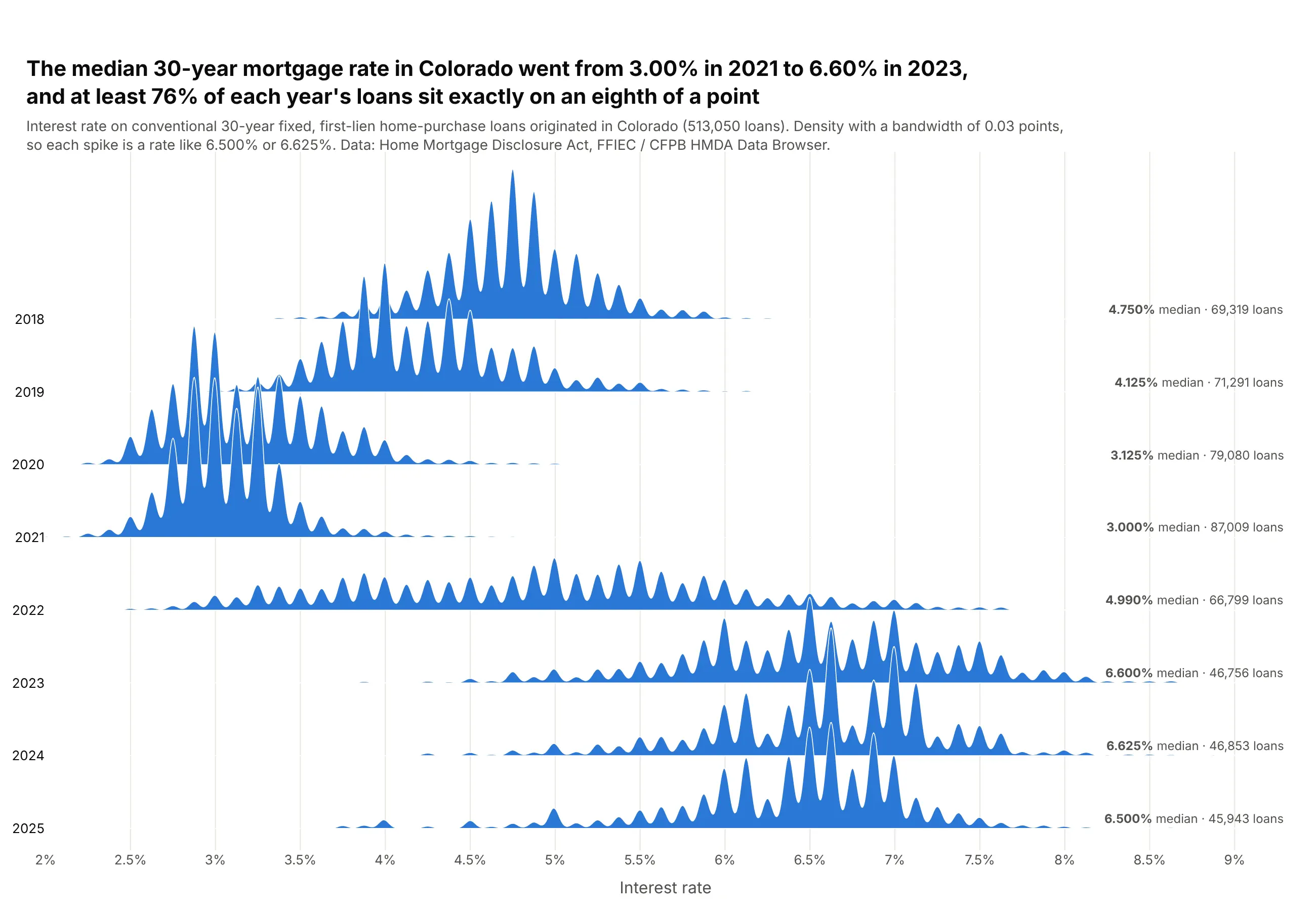
The median rate on a new 30-year fixed loan in Colorado went from 3.00% in 2021 to 6.60% in 2023, across 513,050 loans. A narrow bandwidth turns each year into a comb, because at least 76% of loans sit exactly on an eighth of a point. Data: HMDA, FFIEC / CFPB HMDA Data Browser, 2018-2025.
Tip: count loans per exact rate and pass the counts as KDE weights, so half a million loans become a few hundred rows.
Get the data from the FFIEC / CFPB HMDA Data Browser (Home Mortgage Disclosure Act loan records) for Colorado,2018-2025: originated, first-lien, conventional, 30-year fixed home-purchase loans, and shape it into a table(columns: year, rate in percent, loans = number of loans at that exact rate).Build a plotly ridgeline plot with one row per year, 2018 at the top.- Weighted Gaussian kernel density (weights = loans), shared bandwidth 0.03 points, x from 2% to 9.3%.- Overlap 2.2 rows, one blue fill, white outlines.- Print "<median>% median · <n> loans" at the right end of each row.- Title with the 2021 and 2023 medians and the share of loans on an eighth of a point; cite HMDA.
3. Every US bank's profitability since 2000
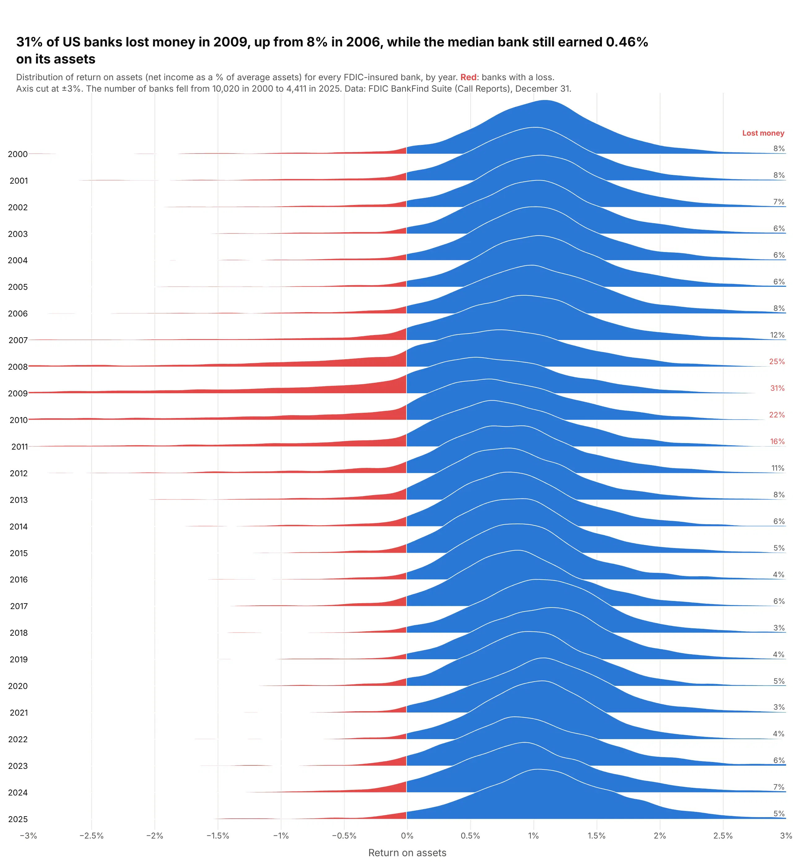
In 2009, 31% of FDIC-insured banks lost money, up from 8% in 2006, while the median bank still earned 0.46% on its assets. The middle barely moves; the crisis is the left tail swelling in 2008-2010. Data: FDIC BankFind Suite (Call Reports), December 31 of each year.
Tip: draw each ridge twice from the same curve, in blue and then clipped to x < 0 in red, so losses read as a shaded tail.
Get the data from the FDIC BankFind Suite API (financials endpoint, Call Report data) for every FDIC-insuredbank at each December 31 from 2000 to 2025, and shape it into a table(columns: year, roa = full-year return on assets in percent).Build a plotly ridgeline plot with one row per year, 2000 at the top, x cut at -3% to +3%.- Kernel density per year (bandwidth 0.08), overlap 2.2, blue fill.- Redraw the part of each ridge left of zero in red on top.- Print the share of banks with roa < 0 at the right of each row, in red when above 15%.- Title with the worst year's share and the median that year; cite FDIC.
Another way to see it: a line of the share of banks losing money gives exact values, but drops the shape of everything else.
4. How long emergency room visits take, hospital by hospital
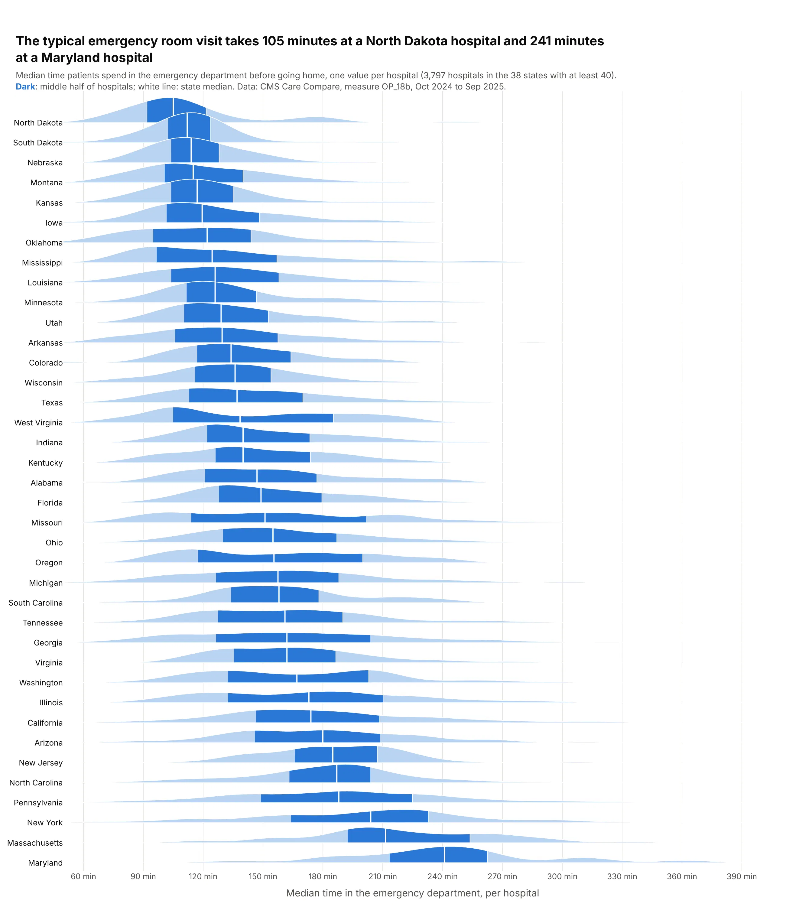
The typical emergency visit takes 105 minutes at a North Dakota hospital and 241 at a Maryland one. The dark band, the middle half of each state's hospitals, spans about 30 minutes in North Dakota and 69 in New York. Data: CMS Care Compare, measure OP_18b, October 2024 to September 2025.
Tip: redraw the 25th-75th percentile part of each ridge in a darker shade, which builds a box plot into every ridge.
Get the data from CMS Care Compare, Timely and Effective Care - Hospital (data.cms.gov dataset yv7e-xc69),measure OP_18b (median minutes patients spend in the emergency department before leaving), and shape itinto a table (columns: facility_id, state, minutes, sample).Build a plotly ridgeline plot with one row per state, keeping states with at least 40 hospitals.- Kernel density per state (bandwidth 12 minutes), x from 50 to 400; overlap 1.5.- Sort by state median, fastest at the top; light blue ridges.- Redraw the part between each state's 25th and 75th percentile in dark blue, and a white line at the median.- Title with the fastest and slowest state medians; cite CMS.
5. The Colorado River before and after Glen Canyon Dam
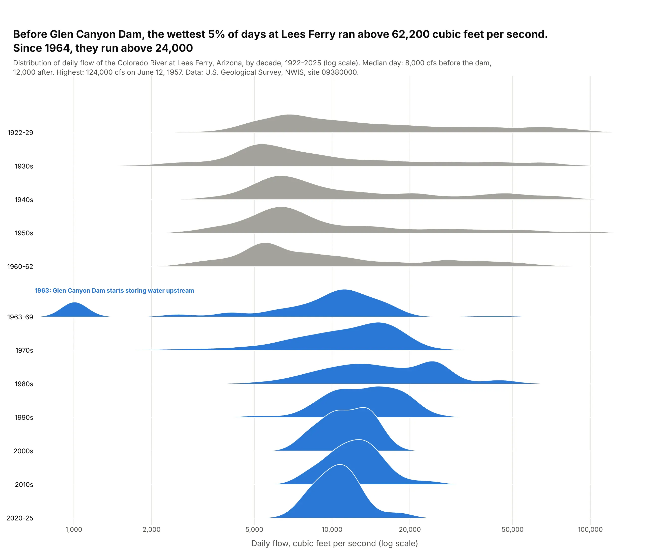
Before Glen Canyon Dam, the wettest 5% of days at Lees Ferry ran above 62,200 cubic feet per second; since 1964, above 24,000. Wide gray ridges of winter lows and spring floods give way to narrow, regulated releases. Data: U.S. Geological Survey NWIS, site 09380000, 1922-2025.
Tip: split the decade where the regime changes (1960-62 and 1963-69) and leave a labeled half-row gap.
Get the data from the U.S. Geological Survey's National Water Information System, daily discharge(parameter 00060, cubic feet per second) at site 09380000, Colorado River at Lees Ferry, Arizona,1922-2025, and shape it into a table (columns: date, cfs).Build a plotly ridgeline plot with one row per decade, splitting the 1960s into 1960-62 and 1963-69.- Kernel density on log10(cfs) (bandwidth 0.05), log x axis from 700 to 150,000; overlap 1.6.- Gray before 1963, blue after; a half-row gap and a label for 1963, when Glen Canyon Dam started storing water.- Title with the 95th percentile before and after; cite USGS.
6. When New Yorkers call 311
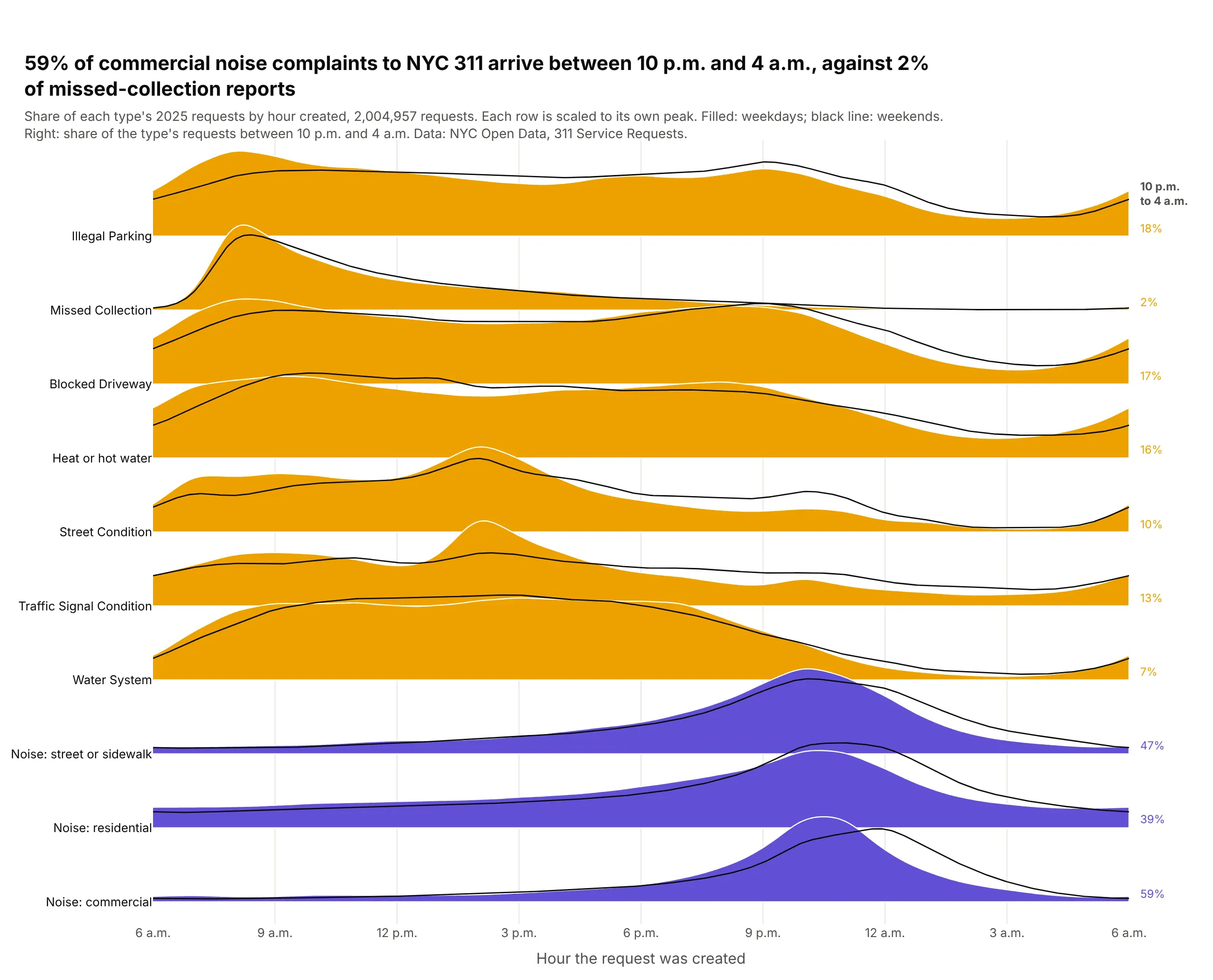
59% of commercial noise complaints to NYC 311 in 2025 arrived between 10 p.m. and 4 a.m., against 2% of missed-collection reports. The types range from 42,977 to 577,253 requests, so each row is scaled to its own peak. Data: NYC Open Data 311 Service Requests, 2,004,957 requests in 2025.
Tip: start a time-of-day axis where activity is lowest (6 a.m. here), so the night isn't split at midnight.
Get the data from NYC Open Data's 311 Service Requests (dataset erm2-nwe9), requests created in 2025 for 10complaint types, counted on the server by hour created and weekday/weekend, and shape it into a table(columns: complaint_type, hour, weekend, requests).Build a plotly ridgeline plot with one row per complaint type and an x axis from 6 a.m. to 6 a.m.- Each row: the share of the type's requests per hour, smoothed with a circular Gaussian (sigma 0.6 hours),scaled to the row's own peak; weekdays filled, weekends as a black line on the same row.- Purple for types with more than 30% of requests between 10 p.m. and 4 a.m., orange otherwise;print that share at the right. Sort rows by peak hour. Cite NYC Open Data.
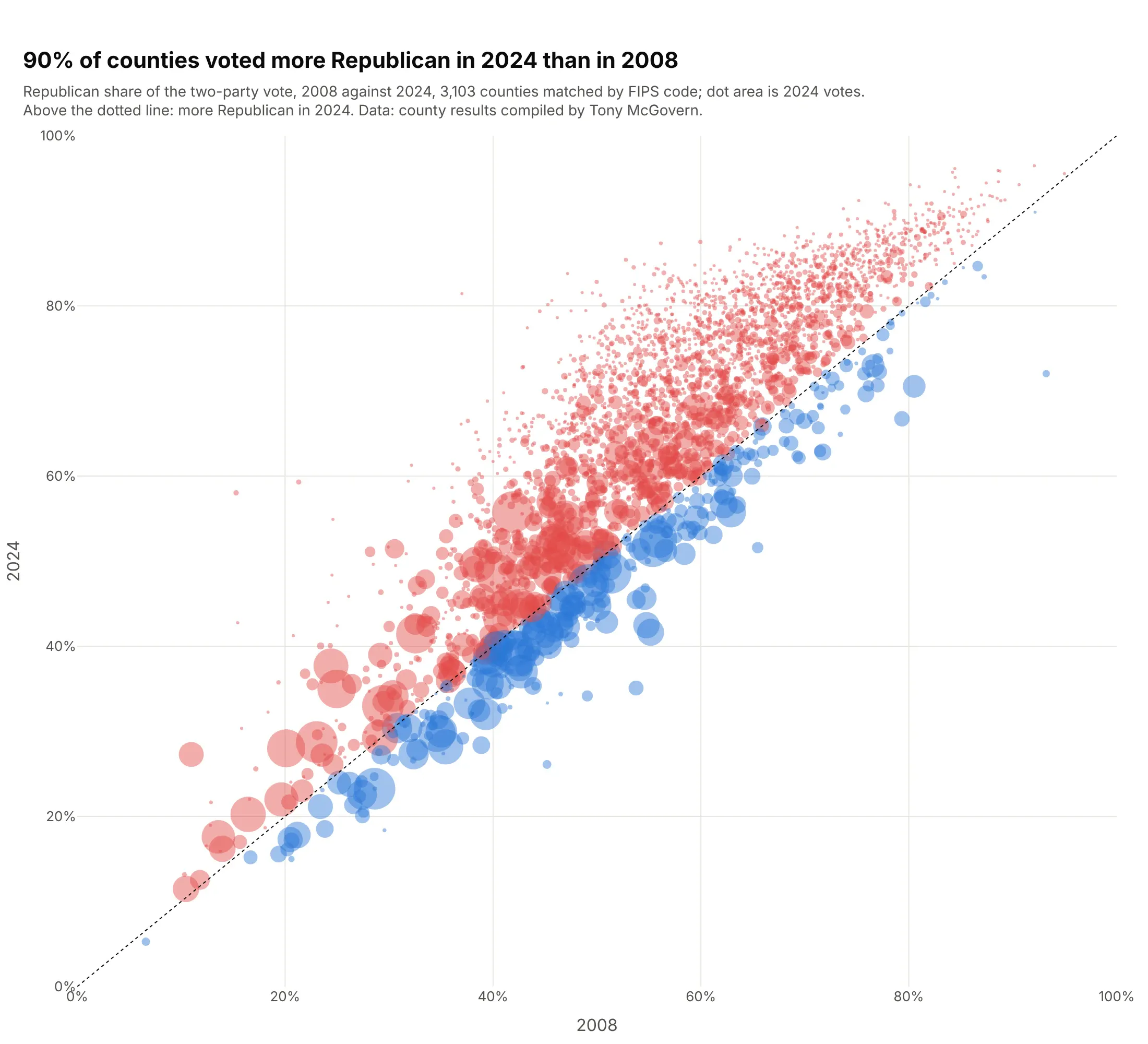
7. How US counties voted, 2008-2024
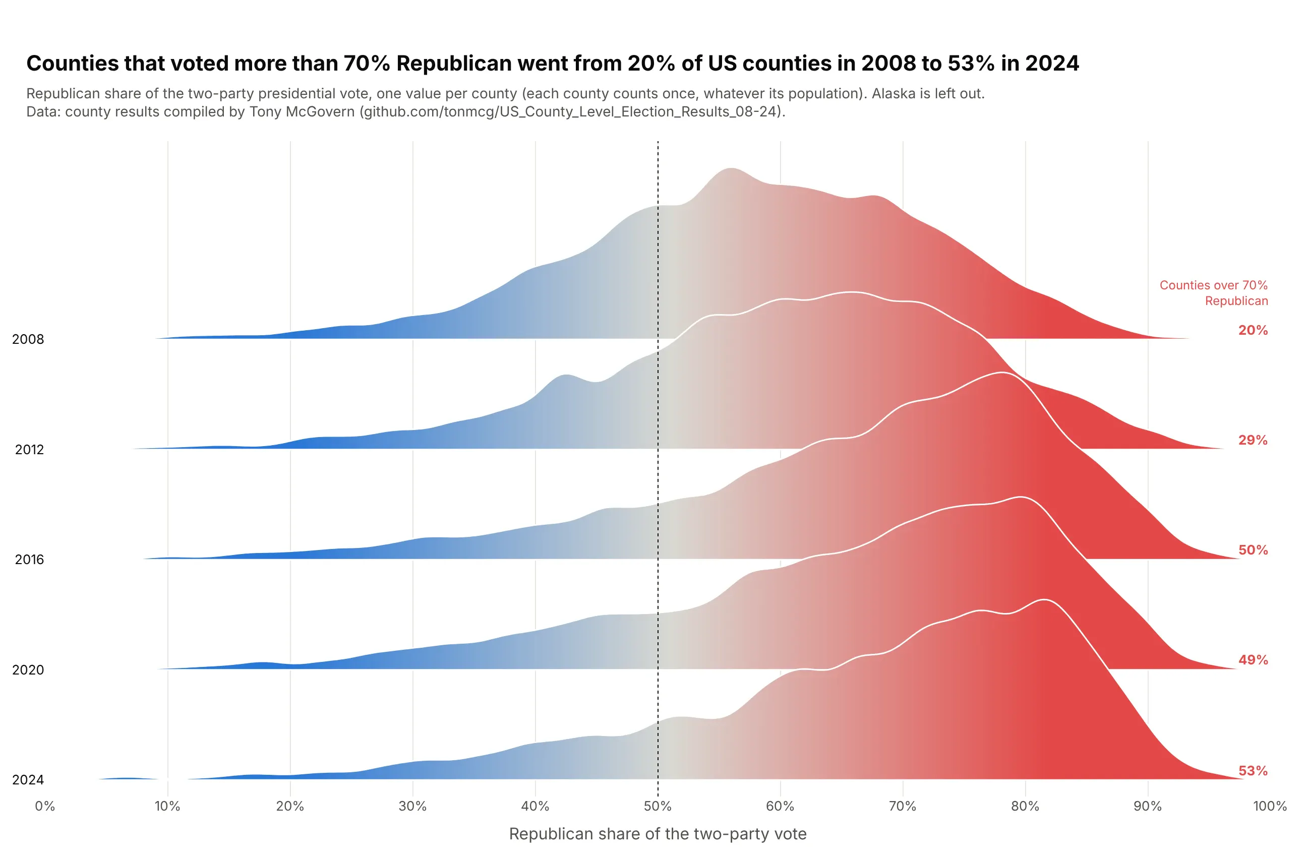
Counties that voted more than 70% Republican went from 20% of US counties in 2008 to 53% in 2024, with the biggest jump in 2016. Each county counts once, so the mass on the right is many small counties. Data: county results compiled by Tony McGovern (tonmcg/US_County_Level_Election_Results_08-24), Alaska left out.
Tip: fillgradient=dict(type="horizontal", start=0.2, stop=0.8, colorscale=...) colors each ridge by its own x position.
Get the data from Tony McGovern's county-level US presidential election results(github.com/tonmcg/US_County_Level_Election_Results_08-24) for 2008-2024, dropping Alaska, and shape it into atable (columns: year, fips, gop_share = Republican / (Republican + Democratic votes), total_votes).Build a plotly ridgeline plot with one row per election, 2008 at the top, x from 0 to 100%.- Kernel density per year (bandwidth 0.015), overlap 1.7, white outlines.- Fill every ridge with fillgradient type "horizontal", start 0.2, stop 0.8, blue #2a78d6 to gray to red #e34948.- Dotted line at 50%; print the share of counties over 70% Republican at the right. Cite the source.
Another way to see it: a scatter of each county's 2008 share against 2024, sized by votes, shows that 90% of counties moved right, and that the big blue metro counties sit below the diagonal.
8. MLB fastballs got faster
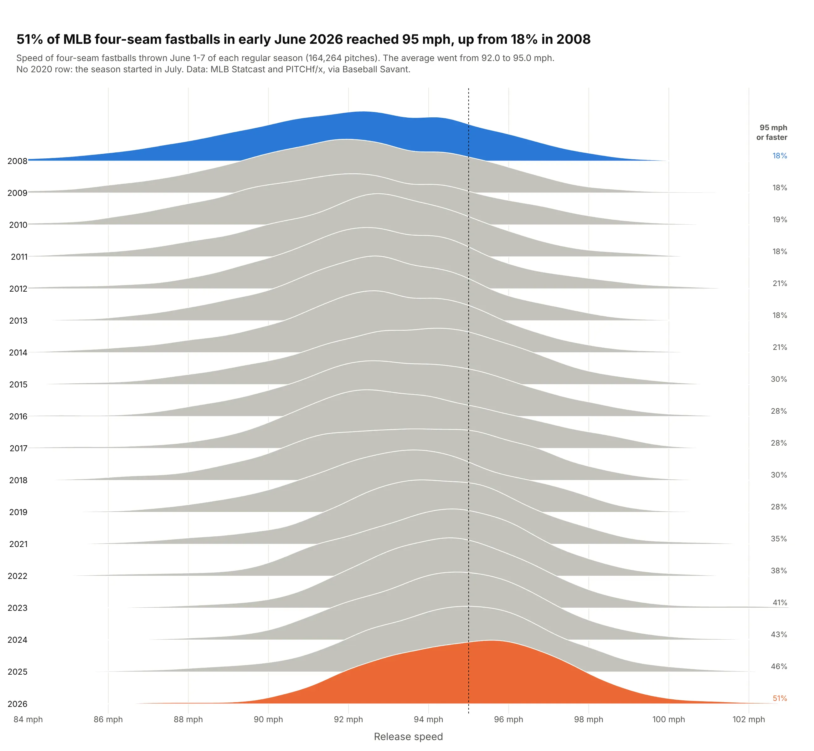
51% of four-seam fastballs in the first week of June 2026 reached 95 mph, up from 18% in 2008, and the average rose from 92.0 to 95.0 mph. The gray rows show a steady drift, not one jump. Data: MLB Statcast and PITCHf/x via Baseball Savant, 164,264 pitches.
Tip: gray every row except the two you compare, and print the share at 95 mph at the end of each row.
Get the data from Baseball Savant's Statcast search export (MLB pitch-by-pitch data): four-seam fastballs(pitch type FF) in regular-season games June 1-7 of each season 2008-2026, counted per 0.1 mph, and shape itinto a table (columns: year, mph, pitches).Build a plotly ridgeline plot with one row per season, 2008 at the top, x from 84 to 103 mph.- Weighted kernel density (weights = pitches, bandwidth 0.45 mph), overlap 2.2.- Light gray ridges except the first season (blue) and the last (orange).- Dotted line at 95 mph; print each season's share at 95 mph or faster at the right. Cite Baseball Savant.
9. How late US airlines landed
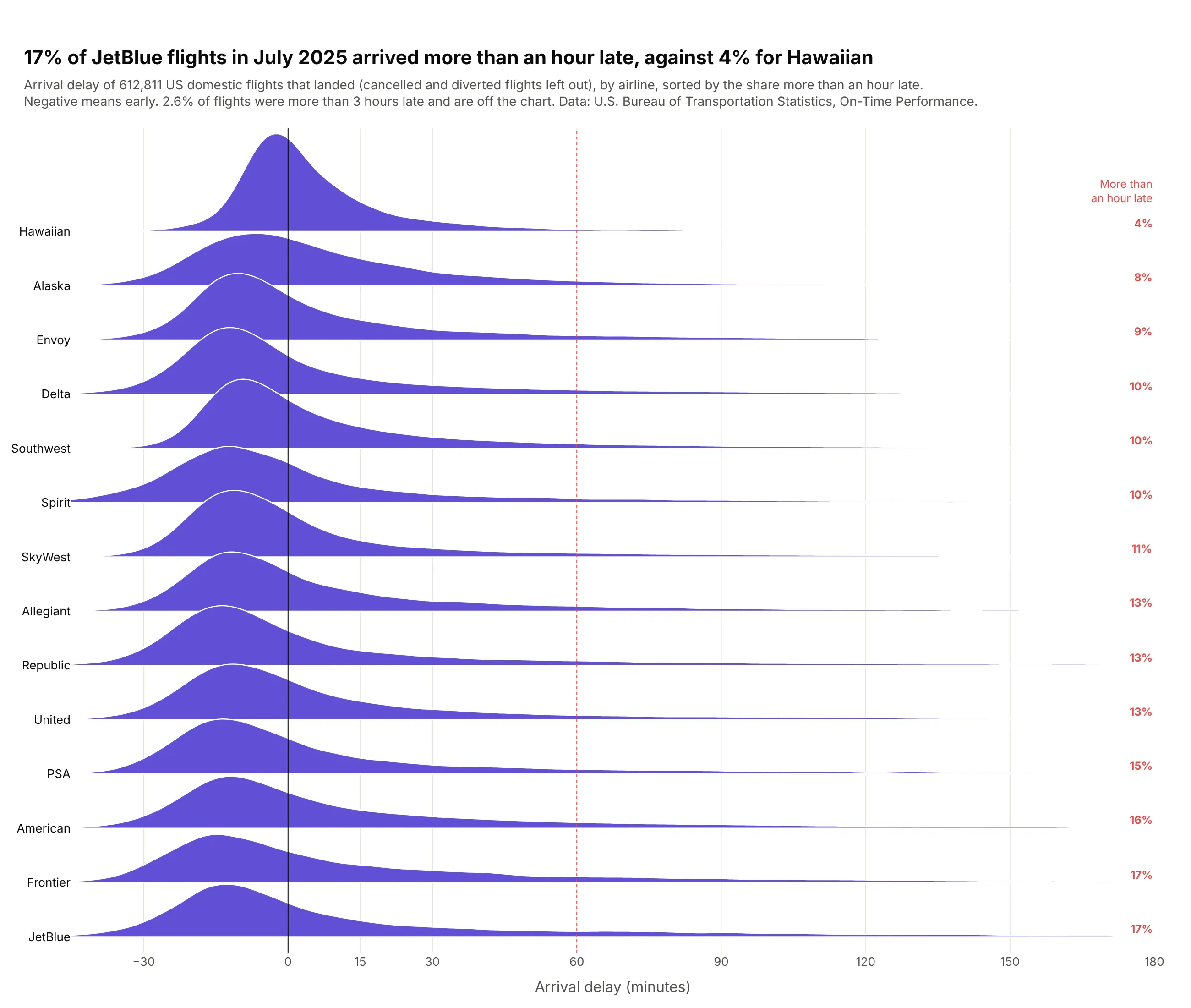
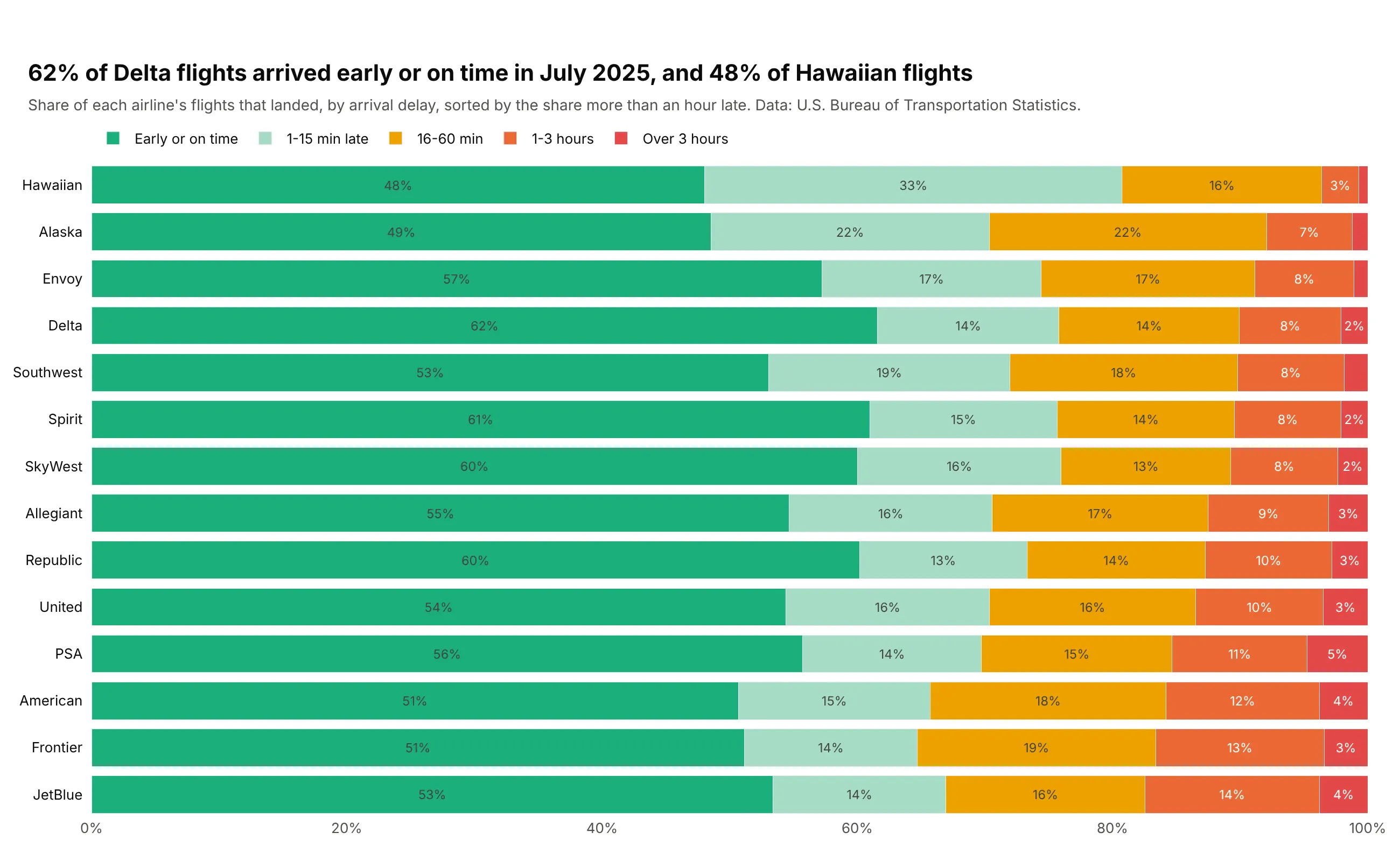
17% of JetBlue flights in July 2025 arrived more than an hour late, against 4% for Hawaiian. Every airline's median is within a few minutes of on time, so the rows are sorted by the tail, where they differ. Data: U.S. Bureau of Transportation Statistics, On-Time Performance, July 2025.
Tip: sort by the statistic people care about, here the share more than an hour late, instead of a median every row shares.
Get the data from the U.S. Bureau of Transportation Statistics' Reporting Carrier On-Time Performance filefor July 2025 (every domestic flight by reporting airline), dropping cancelled and diverted flights, andshape it into a table (columns: carrier, airline, delay_min = arrival delay in minutes, flights).Build a plotly ridgeline plot with one row per airline, x cut at -45 to 180 minutes.- Weighted kernel density (weights = flights, bandwidth 3 minutes), overlap 1.8, purple fill.- Sort rows by the share of flights more than 60 minutes late, lowest at the top; print it at the right.- Lines at 0 and 60 minutes; say in the subtitle how many flights are beyond 3 hours. Cite BTS.
Another way to see it: 100% stacked bars of delay buckets give exact shares per airline, at the cost of the shape inside each bucket.
10. What US developers earn, by role
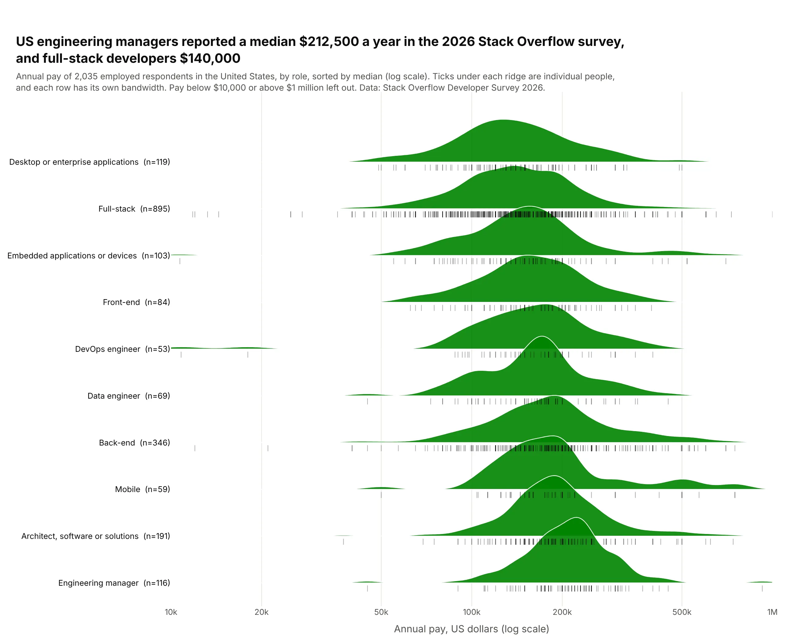
US engineering managers reported a median $212,500 in the 2026 Stack Overflow survey, and full-stack developers $140,000. Some rows are small (53 DevOps engineers against 895 full-stack developers), so ticks under each ridge show every respondent. Data: Stack Overflow Developer Survey 2026, employed US respondents.
Tip: for small rows, add a rug of raw values (symbol="line-ns-open" markers) and put n in the label.
Get the data from the Stack Overflow Annual Developer Survey 2026 public results file, employed respondents inthe United States with ConvertedCompYearly between $10,000 and $1,000,000, the 10 most common roles, and shape itinto a table (columns: devtype, salary_usd).Build a plotly ridgeline plot with one row per role on a log x axis ($10k to $1M).- Kernel density on log10(salary) with a per-row Silverman bandwidth; overlap 1.4; green fill.- Sort rows by median, lowest at the top; label rows "<role> (n=<count>)".- Under each ridge, a rug of every respondent as thin vertical tick markers. Cite Stack Overflow.