
Chris Parmer
November 18, 2026
Confidence Bands - A Complete Guide
TL;DR
- A confidence band is a line chart with a shaded region around the line that shows how uncertain the value of the line is at each point along the x axis, for example the 95% confidence interval (CI) of a global temperature estimate, a trial's mean change from baseline or a fitted calibration curve.
- Confidence bands are also known as error bands, ribbon plots (the ggplot2 geom_ribbon, and matplotlib's fill_between draws the same shape) and, in seaborn's lineplot, the error band of a line chart. They are similar to error bars drawn at every x value, to the nested bands of a fan chart and to the band around a regression plot, and they are a variation on a line chart.
- Four different bands look alike and answer different questions: a confidence band shows how well an average is known, a prediction band shows where one new value will fall, a standard deviation band shows how spread out the data are, and a quantile range shows where a share of the data lies. Say which one you are drawing, because the widths can differ by more than four times, as the sleep study below shows.
- You can make a confidence band with Plotly in Python from two go.Scatter traces with fill="tonexty", or from one trace with fill="toself". Plotly Express has no band argument (its error_y draws a bar at every point), so the code below includes a helper that computes the band from raw data.
What is a confidence band?
Confidence bands look like this:
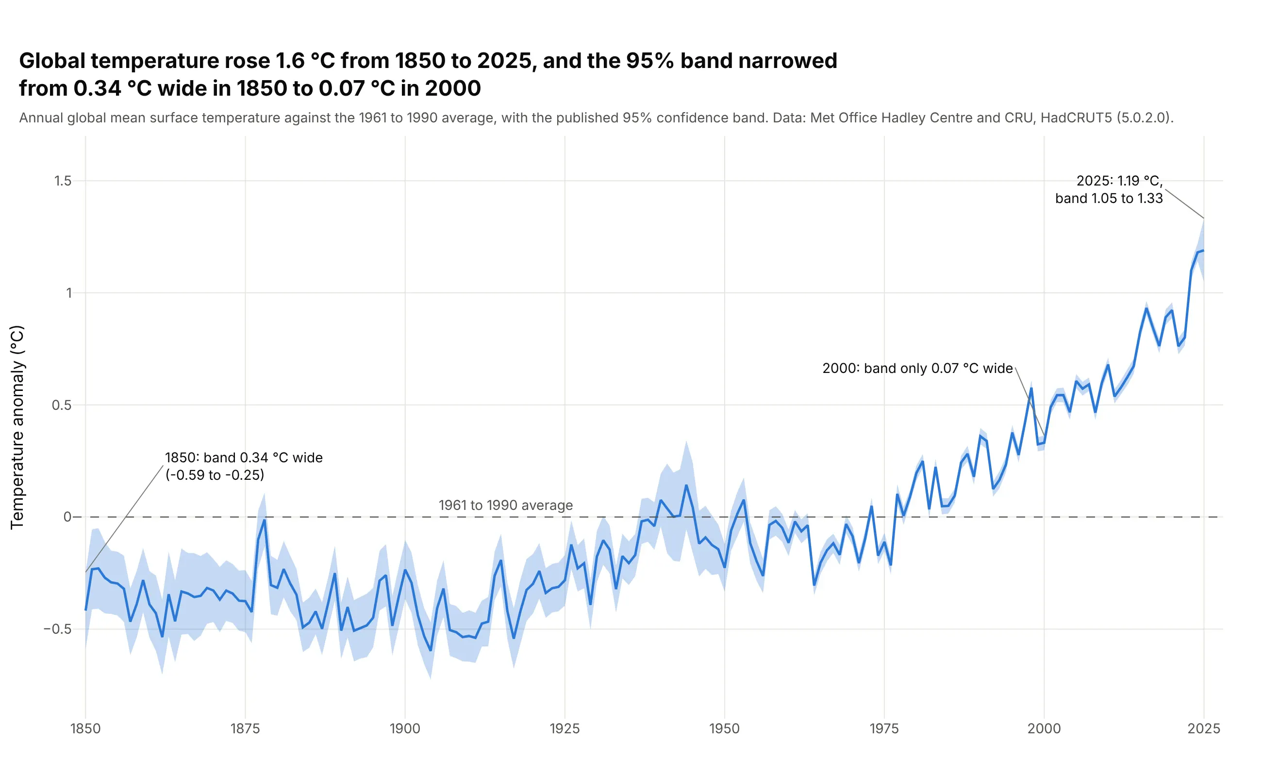
Data: Met Office Hadley Centre and the University of East Anglia Climatic Research Unit (CRU), HadCRUT5 version 5.0.2.0, global annual mean surface temperature anomaly with the published 95% confidence limits.
How do you read a confidence band? In the example above, notice these things:
- The line is the best estimate of global temperature for each year, written as an anomaly (the difference from the 1961 to 1990 average). It was -0.42 °C in 1850 and 1.19 °C in 2025, a rise of 1.6 °C.
- The band is the 95% confidence interval the Met Office publishes for each year's estimate. It says how well that year's global average is known, and not how much the weather varied from one year to the next.
- The band is 0.34 °C wide in 1850 and 0.07 °C wide in 2000, which fits the much sparser measurements of the early record (our reading; the Met Office describes its method in the dataset documentation). Where the band is narrow, a wiggle in the line is easier to trust as a real change, and where it is wide, a wiggle may be measurement error.
- The band is not always narrowing: the 2025 band is 0.28 °C wide, against 0.08 °C for 2024.
It's often used for charts like these:
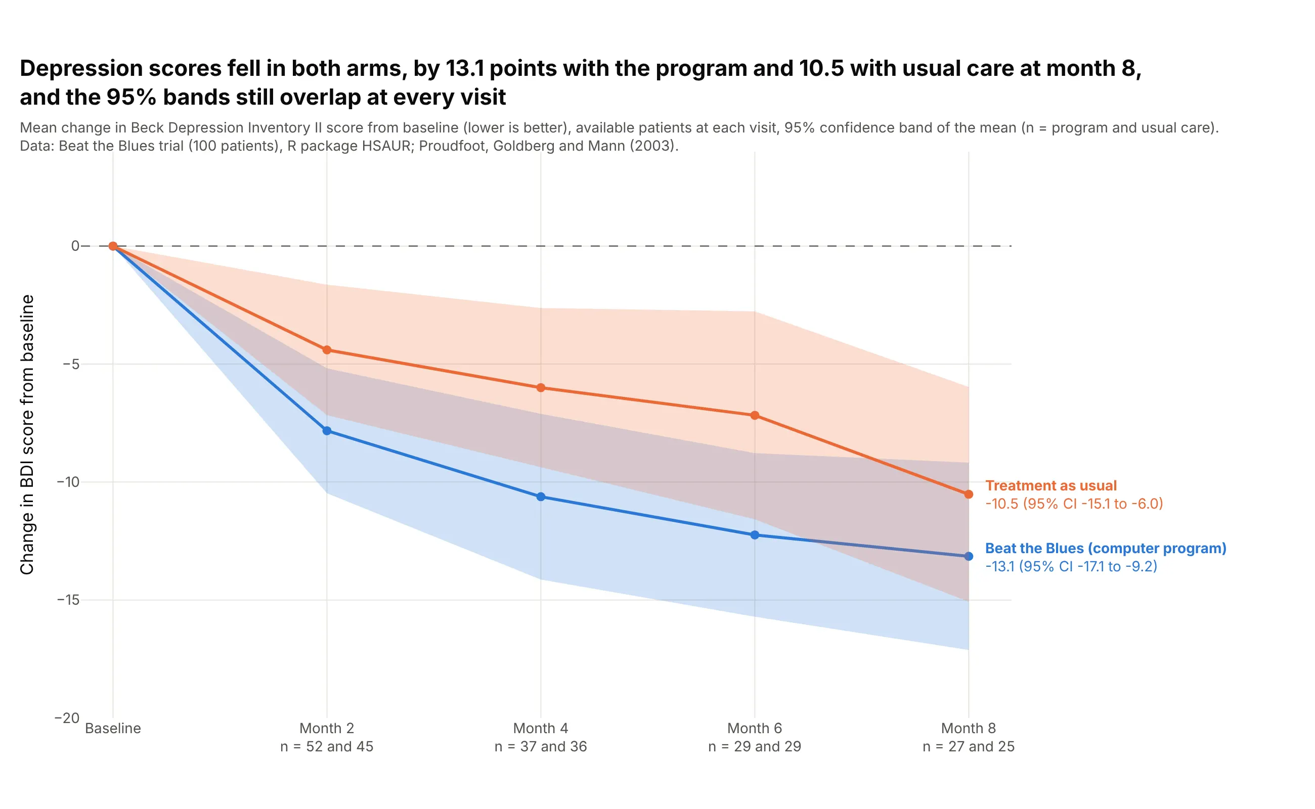
Clinical trials. A trial report shows the mean change from baseline in each arm with its 95% CI at every visit. In the Beat the Blues trial of a computer-based therapy program for depression, scores fell by 13.1 points with the program and 10.5 with usual care at month 8, and the two bands overlap at every visit. Only 27 of 52 and 25 of 48 patients had a score at month 8, so the bands are wider than at month 2 (52 and 45 patients). Data: Beat the Blues trial (100 patients), R package HSAUR (Everitt and Hothorn); Proudfoot, Goldberg and Mann (2003). The change and the bands are our own calculation from the available scores, without filling in missing ones.
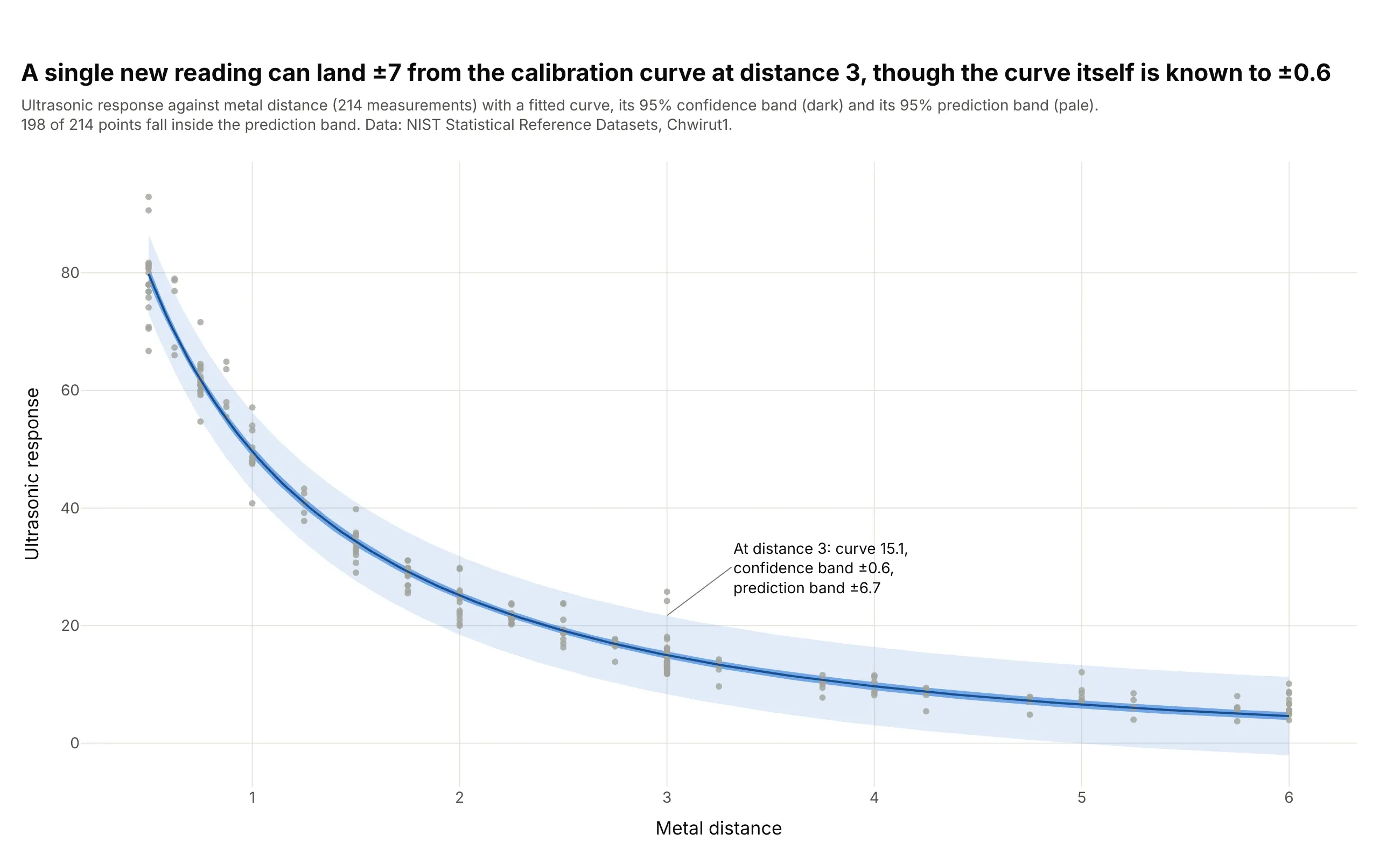
Calibration curves. The classic use for two bands on one chart is a calibration, where an instrument's reading is related to a known quantity so that later readings can be converted back. The National Institute of Standards and Technology (NIST) reference data on ultrasonic response against metal distance has 214 measurements. At distance 3 the fitted curve is 15.1, its 95% confidence band is ±0.6 and its 95% prediction band is ±6.7, and the prediction band is the one to use for a new reading. Data: NIST Statistical Reference Datasets, Chwirut1 (214 observations, nonlinear regression).
Four bands that look alike
A shaded band can mean four different things, and the chart rarely says which. The sleep study below shows all four on the same data: the reaction time of 18 people over 10 days of sleep restriction, with each person as a thin gray line:
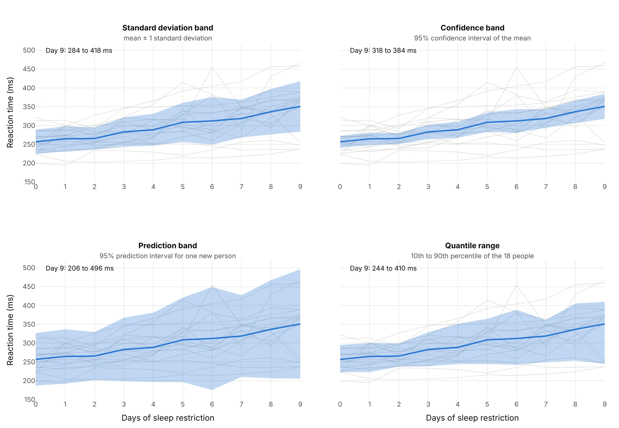
Data: R package lme4, sleepstudy (Belenky et al., 2003, the group limited to three hours in bed per night; 18 people, days 0 to 9).
The mean reaction time on day 9 is 351 milliseconds, and the four bands around it are:
- Standard deviation band (284 to 418 ms). The mean plus and minus one standard deviation (the typical distance of a person from the mean). It describes the spread of the data, so it does not shrink when you add people. About two thirds of a bell-shaped set of values fall inside it, and 12 of the 18 people are inside it on day 9.
- Confidence band (318 to 384 ms). The mean plus and minus a t value times the standard deviation divided by the square root of the number of people, so mean ± t × s / √n, where t is 2.11 for 95% with 18 people. It describes how well the mean is known, and it narrows as n grows. It is a band for the average and not for a person, so only 10 of the 18 people are inside it on day 9 (between 6 and 10 on every day).
- Prediction band (206 to 496 ms). The mean plus and minus t × s × √(1 + 1/n), so it holds the spread of a single new person as well as the uncertainty of the mean. It is the widest of the four, about 4.4 times as wide as the confidence band here (290 ms against 67 ms), it holds all 18 people on day 9 and it stays wide however many people you add.
- Quantile range (244 to 410 ms). The 10th and 90th percentile of the 18 people, so about 80% of this sample lies inside it (14 of 18 on day 9). It needs no bell curve, so it can be lopsided, and it is the band used for the sea ice example below.
The seaborn documentation draws the same line between "measures of data spread" (standard deviation, percentile interval) and "measures of estimate uncertainty" (standard error, confidence interval) in its error bars tutorial. A confidence band belongs to the second group, and the other three bands are often called confidence bands by mistake.
What a 95% confidence interval means
A 95% confidence interval comes from a recipe: if you could repeat the whole measurement many times and build an interval each time with the same recipe, about 95% of those intervals would contain the true value. It is not a statement that the true value has a 95% chance of lying in the one interval on your chart, and it does not say that 95% of the data fall inside.
Pointwise and simultaneous bands
Most bands are pointwise: each x value has its own 95% interval, so the interval is right 95% of the time at any one x, but the whole curve lies inside the band less often, because a curve can leave the band at one point and return. A simultaneous band is built so the whole curve lies inside with 95% probability, and it is wider (Wikipedia explains the difference and lists the methods). The bands in this guide are pointwise, as is almost every band in a chart library.
Where the band comes from
The band can come from the data source, a formula or a resampling method, and the fastest way to trust or doubt a band is to know which:
- Published by the source. The HadCRUT5 temperature example above draws the Met Office's own limits, so you draw them and do not compute them.
- A formula. A t interval for a mean (the clinical trial and the sleep study), or the standard error of a fitted curve (the calibration curve), as in the Python code below.
- A bootstrap. Resample the data with replacement thousands of times, compute the mean each time and take the 2.5th and 97.5th percentile. Seaborn's lineplot does this by default, with errorbar=("ci", 95) and 1,000 resamples (lineplot documentation), as example 3 shows.
- A spread or a quantile. A standard deviation (Bollinger bands, example 4) or a percentile of a reference period or an ensemble of forecasts (examples 1 and 2). These are not confidence intervals, and calling them that is a common mistake.
A short history
The shaded band around a fitted line comes from regression analysis. Holbrook Working and Harold Hotelling published a band for a fitted straight line in 1929, Applications of the Theory of Error to the Interpretation of Trends in the Journal of the American Statistical Association, which holds for all x at once, the kind of simultaneous band described above. Plotting software later made the shape a built-in: ggplot2's geom_ribbon "displays a y interval defined by ymin and ymax" for each x value, matplotlib's fill_between fills the area between two curves, and seaborn's lineplot draws a bootstrapped band by default. We could not find the data behind the 1929 figures in a public form, so there is no redraw of the original here.
Alternatives to a confidence band
Here's the same temperature record drawn six ways. Some are better for the question, some worse, some just different:
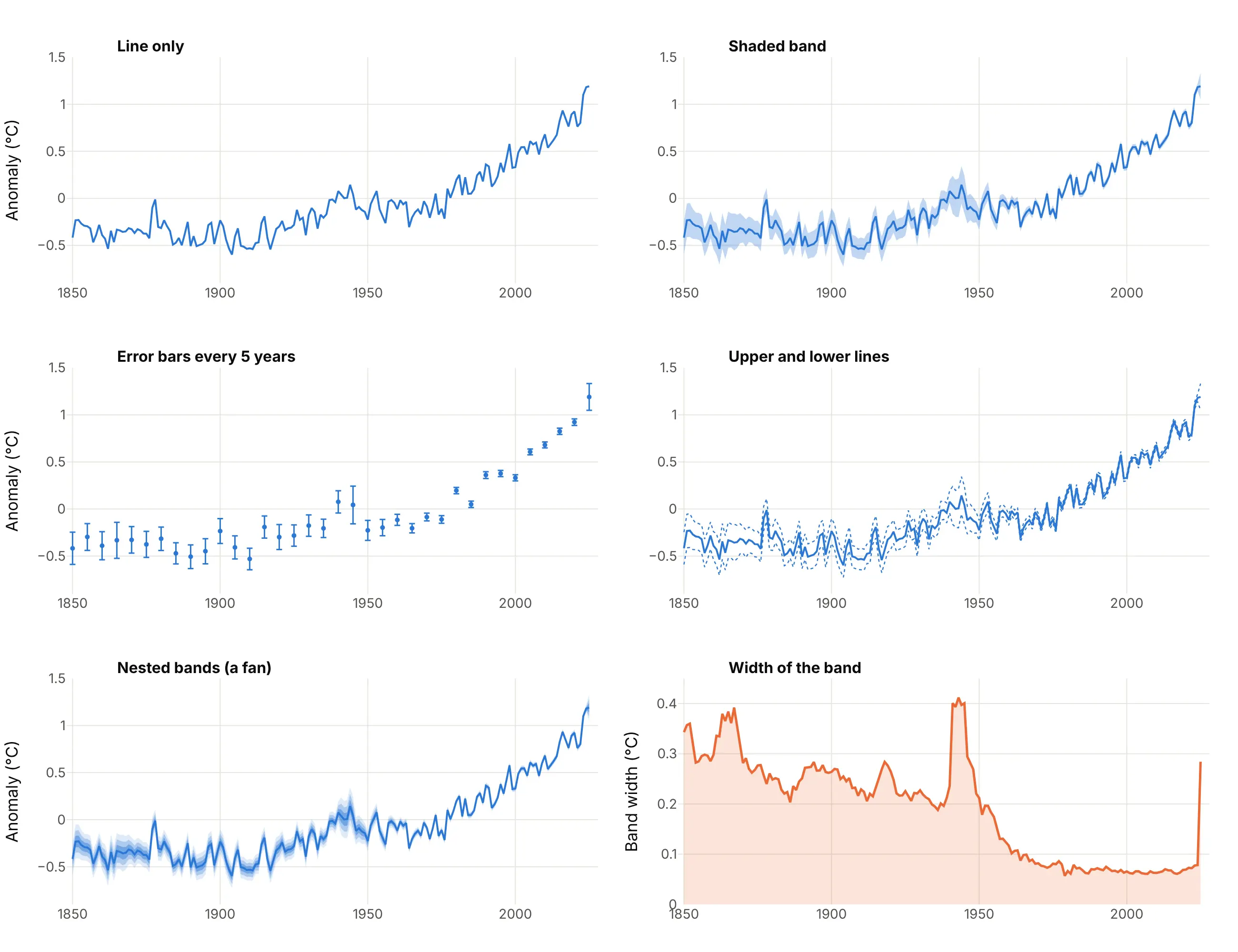
- Shaded band (best for a continuous series). It shows the estimate and its uncertainty at every x at once, and it keeps the line the first thing the eye sees.
- Line only (worse). It looks cleaner and hides everything the reader needs to know about whether a wiggle is real.
- Error bars (works too, at a few x values). They are better for exact limits at chosen points, such as every fifth year, and worse for a series with hundreds of points, where they become a picket fence.
- Upper and lower lines (works too, but harder to read). The two dotted lines carry the same limits, but they look like two more data series and they are easy to read as best and worst cases.
- Nested bands (different). A fan chart draws several levels of the same distribution, such as 50%, 80% and 95%. It is the right choice for a forecast, where the likely range matters as well as the outer limit. Here it assumes a normal curve, which we derived from the 95% limits, so it is an illustration and not a published result.
- Width of the band on its own (different). An area chart of the band width answers one question, how the uncertainty changed, which the band shows only indirectly. It makes the 1940s bump and the 2025 jump easy to see.
Confidence band or fan chart?
A fan chart is a line chart with prediction bands, so it looks like a confidence band with several shades, but the two answer different questions. A confidence band says how well an estimate of something that exists (the average of a measurement, a fitted curve, last year's temperature) is known, and it narrows as data accumulate. A fan chart says where a future value is likely to fall, it holds the scatter of a single outcome and it widens with the forecast horizon however much data you have. When the band is about the future, use the fan chart guide, and when it is about an estimate from data you already have, use a confidence band. The regression plot guide shows both bands around one fitted line.
How to make a confidence band
With AI
ChatGPT, Claude Code, GitHub Copilot, Cursor and other AI tools are excellent at writing Plotly code. Name Plotly in the prompt, and say where the band comes from:
Make a plotly line chart with a confidence band from hadcrut5.csv (columns: year, anomaly, lower, upper; lower and upper are the published 95% limits).- Draw the band first as one go.Scatter polygon with fill="toself" (the years forward along the upper limit, then backward along the lower limit),in the line color at opacity 0.25, with line width 0 and hoverinfo="skip".- Draw the anomaly as a blue line on top, with the band limits in the hover text (customdata and hovertemplate).- Add a dashed zero line labeled "1961 to 1990 average", a title that states the takeaway, and axis titles "Year" and "Temperature anomaly (°C)".- Check: print the band width for 1850, 2000 and 2025.
With Plotly Studio
Plotly Studio is a product for creating data visualizations and Dash apps and for analyzing data with AI, available as a desktop app or embedded in Dash apps. Ask for a confidence band the same way:
Show the mean change in depression score from baseline at each visit for each treatment arm, with a 95% confidence band around each line, and a dropdown to switch between 95% and 90% bands.
In Python or JavaScript
This is the code AI tools write under the hood. When the data source already gives lower and upper limits, a confidence band is two invisible lines and a fill between them. The upper line goes first, and the lower line fills up to the trace before it with fill="tonexty":
import pandas as pdimport plotly.graph_objects as godf = pd.read_csv("hadcrut5.csv") # columns: year, anomaly, lower, upper (the published 95% limits)fig = go.Figure()fig.add_trace(go.Scatter(x=df.year, y=df.upper, mode="lines", line=dict(width=0), hoverinfo="skip", showlegend=False)) # upper edge, drawn first and invisiblefig.add_trace(go.Scatter(x=df.year, y=df.lower, mode="lines", line=dict(width=0), hoverinfo="skip", showlegend=False,fill="tonexty", fillcolor="rgba(42,120,214,0.25)")) # lower edge, filled up to the trace before itfig.add_trace(go.Scatter(x=df.year, y=df.anomaly, mode="lines", line=dict(color="#2a78d6", width=2.5), name="Annual mean"))fig.update_layout(title="Global temperature anomaly with its 95% band", xaxis_title="Year", yaxis_title="Anomaly (°C)")fig.show()
When you have raw observations (one row per person or per run), compute the mean and its band first. The helper below returns a figure with the line and a 95% band from a t interval, and it draws the band as one closed polygon with fill="toself", which does not depend on the order of the traces:
import numpy as npimport pandas as pdimport plotly.graph_objects as gofrom scipy import statsdef line_with_band(df, x, y, level=0.95, color="#2a78d6"):"""Mean of y at each x with a t-based confidence band of the mean, from long data (one row per observation)."""g = df.groupby(x)[y].agg(["mean", "std", "count"])half = stats.t.ppf(0.5 + level / 2, g["count"] - 1) * g["std"] / np.sqrt(g["count"])xs = list(g.index)fig = go.Figure()fig.add_trace(go.Scatter(x=xs + xs[::-1], y=list(g["mean"] + half) + list((g["mean"] - half)[::-1]), fill="toself",fillcolor="rgba(42,120,214,0.25)", line=dict(width=0), hoverinfo="skip", name=f"{level:.0%} confidence band"))fig.add_trace(go.Scatter(x=xs, y=g["mean"], mode="lines", line=dict(color=color, width=3), name="Mean"))return figdf = pd.read_csv("fmri.csv") # columns: subject, timepoint, event, region, signalfig = line_with_band(df[(df.region == "parietal") & (df.event == "stim")], "timepoint", "signal")fig.update_layout(xaxis_title="Timepoint", yaxis_title="Signal")fig.show()
For a fitted line, statsmodels returns both the confidence band and the prediction band, so the chart can show the two together. In summary_frame, mean_ci_lower and mean_ci_upper are the confidence band of the line, and obs_ci_lower and obs_ci_upper are the prediction band for a single new observation:
import pandas as pdimport plotly.graph_objects as goimport statsmodels.api as smdf = pd.read_csv("hadcrut5.csv") # columns: year, anomaly, lower, upperdf = df[df.year >= 1980]fit = sm.OLS(df.anomaly, sm.add_constant(df.year)).fit()pred = fit.get_prediction(sm.add_constant(df.year)).summary_frame(alpha=0.05) # 95% intervalsdef band(fig, x, low, high, rgba, name):fig.add_trace(go.Scatter(x=list(x) + list(x)[::-1], y=list(high) + list(low)[::-1], fill="toself", fillcolor=rgba,line=dict(width=0), hoverinfo="skip", name=name))fig = go.Figure()band(fig, df.year, pred.obs_ci_lower, pred.obs_ci_upper, "rgba(42,120,214,0.12)", "95% prediction band") # where one new year may fallband(fig, df.year, pred.mean_ci_lower, pred.mean_ci_upper, "rgba(42,120,214,0.35)", "95% confidence band") # where the trend line isfig.add_trace(go.Scatter(x=df.year, y=df.anomaly, mode="markers", marker=dict(color="#0b0b0b", size=6), name="Annual mean"))fig.add_trace(go.Scatter(x=df.year, y=pred["mean"], mode="lines", line=dict(color="#2a78d6", width=3), name="Trend"))fig.show()
Plotly Express can draw error bars on a line but has no argument for a band. In Plotly 7.1.0, px.line(df, x="year", y="anomaly", error_y="up", error_y_minus="down") draws a bar at every point, which is the error bars chart and not a band, so build a band with the go.Scatter code above and, if you like Plotly Express for the rest, add its traces to the same figure with fig.add_traces(...).
In JavaScript, plotly.js draws the same chart with the same two-trace fill. This example uses the treatment as usual arm of the Beat the Blues trial, with the mean change in depression score and its 95% limits at each visit:
<div id="chart"></div><script src="https://cdn.plot.ly/plotly-4.1.1.min.js"></script><script>// Beat the Blues trial: mean change in depression score from baseline and its 95% confidence limits, treatment as usualconst month = [0, 2, 4, 6, 8];const mean = [0, -4.40, -6.00, -7.17, -10.52];const lower = [0, -7.16, -9.37, -11.58, -15.07];const upper = [0, -1.64, -2.63, -2.77, -5.97];Plotly.newPlot("chart", [{type: "scatter", mode: "lines", x: month, y: upper, line: {width: 0}, hoverinfo: "skip", showlegend: false}, // upper edge, invisible{type: "scatter", mode: "lines", x: month, y: lower, line: {width: 0}, fill: "tonexty", fillcolor: "rgba(235,104,52,0.25)",hoverinfo: "skip", showlegend: false}, // lower edge, filled up to the upper edge{type: "scatter", mode: "lines+markers", x: month, y: mean, line: {color: "#eb6834", width: 3}, name: "Treatment as usual"}], {width: 900, height: 520, title: {text: "Change in depression score from baseline, with a 95% band"},xaxis: {title: {text: "Months since baseline"}}, yaxis: {title: {text: "Change in score"}}});</script>
Share it
Every Plotly chart has a Share chart button (the cloud icon in its toolbar) that uploads it to Plotly Cloud and gives you a link. Only you can see it until you change its visibility.
For a live app, put the chart in a Dash app and publish it with the Plotly Cloud command-line interface (CLI). Coding agents can run these commands for you:
pip install "dash[cloud]"plotly user loginplotly app publish
If your data has to stay in your own cloud or data center, publish to Dash Enterprise instead.
Dos and don'ts
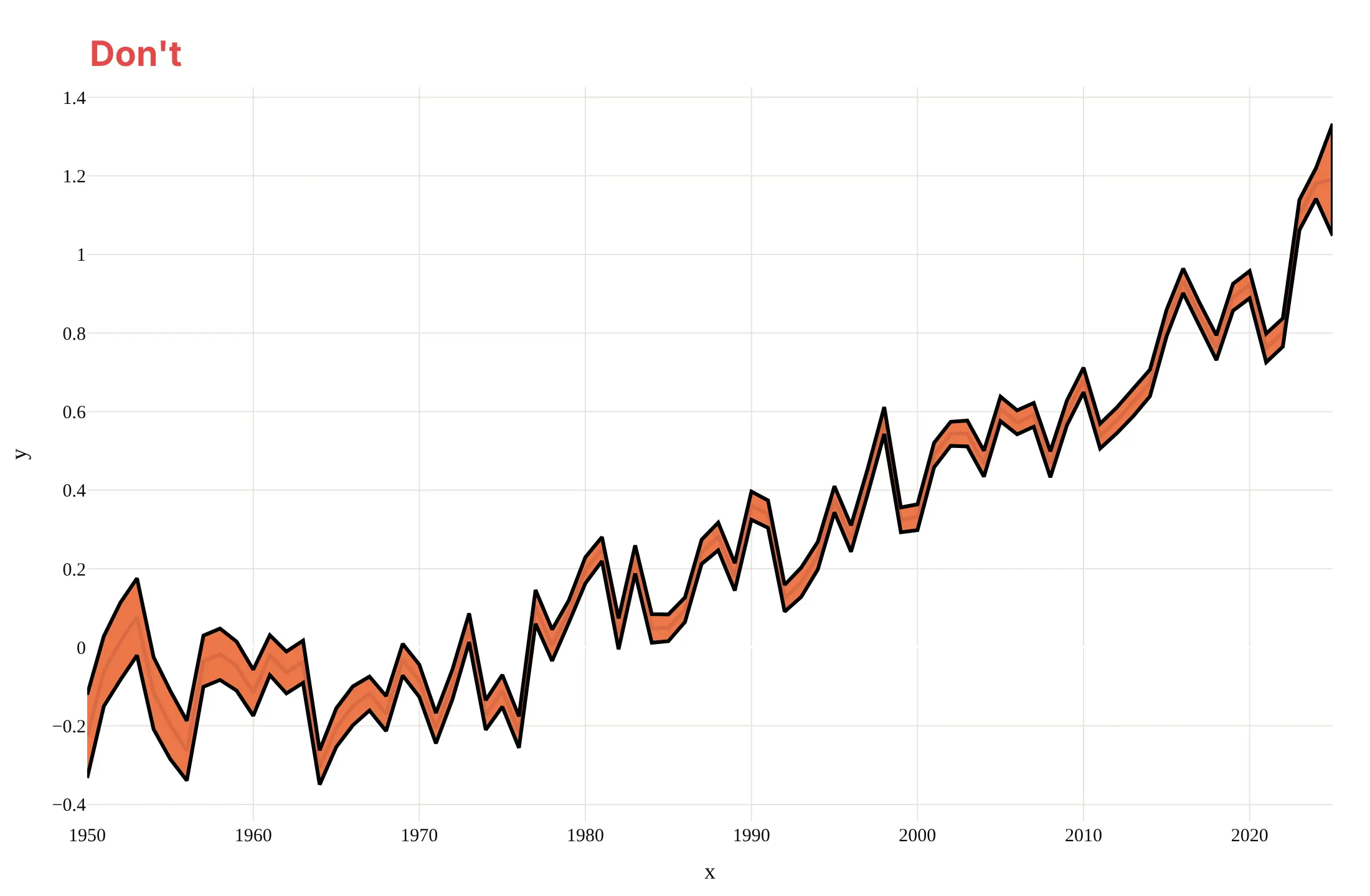
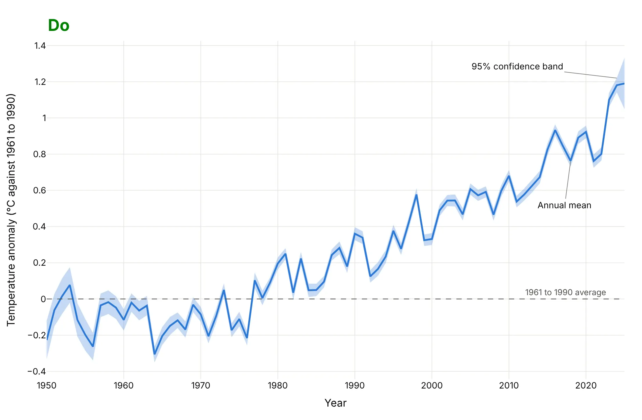
A confidence band is easy to draw and easy to draw badly, because the shading can hide the line and the reader cannot tell what the band holds. Here is the temperature record from 1950 both ways, with the same blue line and the same data.
Don't draw the band in an opaque color on top of the line, outline it with a heavy black stroke, leave the axes as x and y, keep a serif font, or leave out what the band holds:
Do draw a translucent band behind the line with no outline, label the band and the line directly, mark the zero line the reader compares with, and write axis titles in words with units:
Checklist
Do
- Say what the band is in the subtitle or a label ("95% confidence interval of the mean", "10th to 90th percentile of 1981 to 2010") and where it comes from.
- Draw the band first, translucent and without an outline, and the line on top.
- Use the same color as the line, so the band reads as part of it.
- Draw the prediction band as well when readers will use the chart to judge a single new value.
- Mark the reference the reader compares with (zero change, a target, a normal range).
- Say how many observations lie behind each point when the number changes (the n under the trial's visits).
Don't
- Call a standard deviation or a percentile band a confidence interval.
- Read overlapping bands as "no difference". Two 95% intervals can overlap while the difference between the groups is still clear, so test the difference or plot it.
- Compare the band with the individual data points as if the band were meant to hold them. A confidence band should leave most points outside.
- Hide the n. A narrow band from 5 observations and a narrow band from 5,000 are not the same claim.
More confidence band examples
Five more charts built from real public data, each with its source, the technique that makes it work and a prompt to rebuild it.
1. A forecast band from 51 ensemble members: Houston temperature
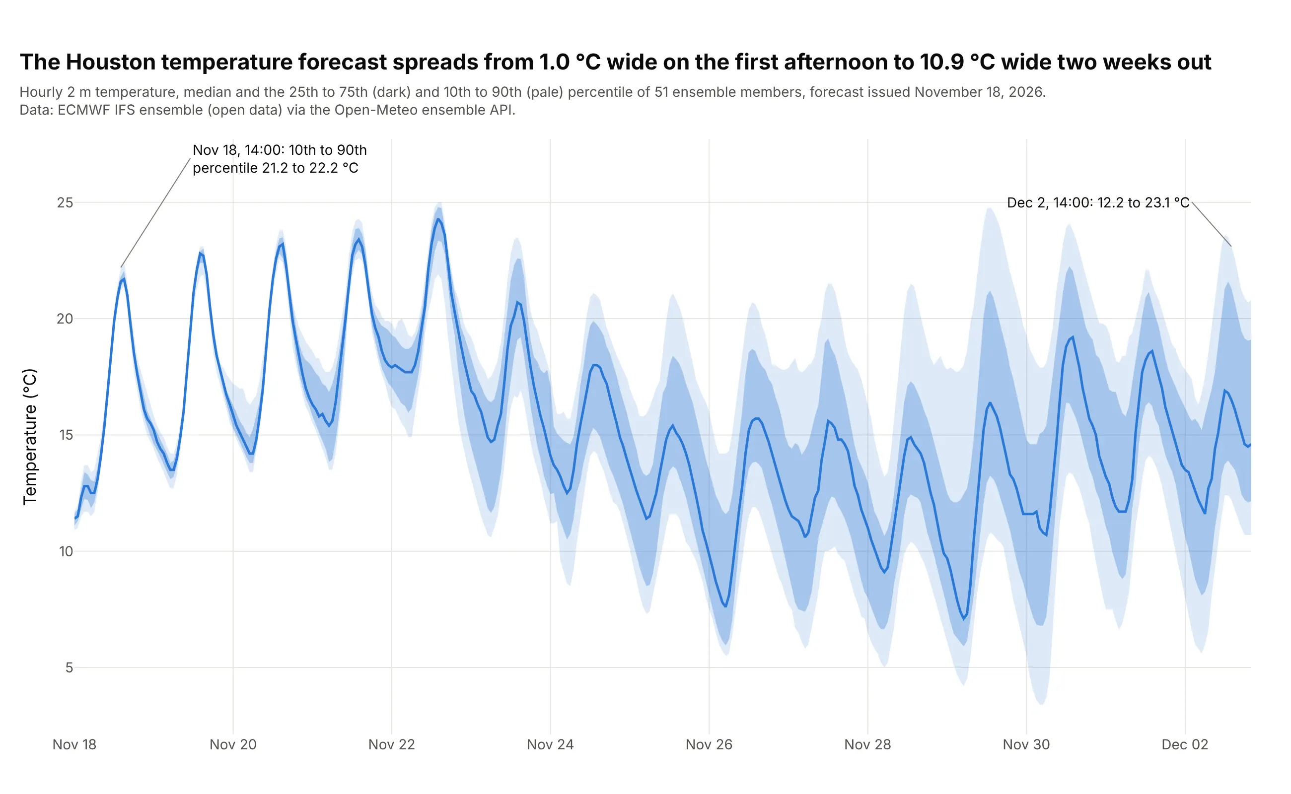
A weather forecast is run 51 times from slightly different starting conditions, and the spread between the runs is the band. The 10th to 90th percentile of the 51 members is 1.0 °C wide at 14:00 on November 18 (21.2 to 22.2 °C) and 10.9 °C wide at 14:00 on December 2 (12.2 to 23.1 °C). Temperature drives electricity and gas demand, so this is the kind of band an energy analyst would check, and the same chart works for wind speed. Data: European Centre for Medium-Range Weather Forecasts (ECMWF) IFS ensemble (open data) through the Open-Meteo ensemble API, forecast issued November 18, 2026.
Tip: use quantiles of the members and not a mean plus a standard deviation, so the band can be lopsided on a day when one weather pattern is much warmer than the rest.
Get the data from the Open-Meteo ensemble API (ensemble-api.open-meteo.com/v1/ensemble, model ecmwf_ifs025, hourly temperature_2m for Houston at 29.76, -95.37, 15 forecast days,which returns one column per ensemble member: 51 members) (columns after reshaping: time, member, temp_c).Build a plotly chart of the median across members as a blue line, with a band from the 25th to the 75th percentile and a paler band from the 10th to the 90th percentile at each hour,drawn as fill="toself" polygons in the same blue. Title it with the width of the 10th to 90th band on the first and last afternoon.
2. A range band from history: Arctic sea ice extent
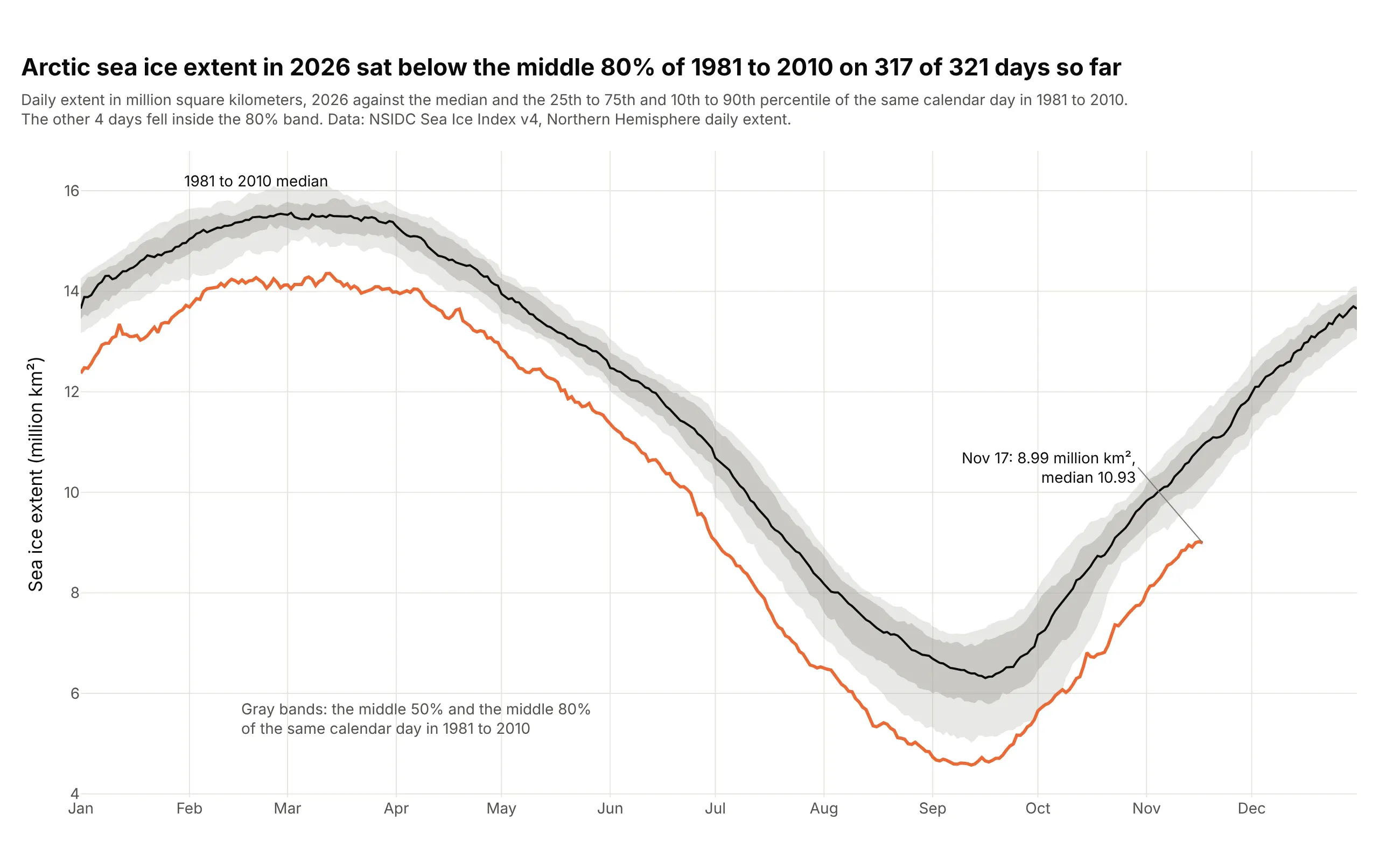
The National Snow and Ice Data Center (NSIDC) draws each year's daily sea ice extent in its Charctic graph against the median of 1981 to 2010, with the interquartile range (the middle 50% of values for that date) and the interdecile range (the middle 80%) as gray bands. In 2026 the extent was below the 10th percentile of the reference years on 317 of 321 days so far, and on November 17 it was 8.99 million square kilometers against a median of 10.93. The band describes how the reference years varied, so it is a quantile range, not a confidence interval of anything. Data: NSIDC Sea Ice Index version 4, Northern Hemisphere daily extent (every other day before mid-1987, filled by linear interpolation for the reference years).
Tip: put the current year in a strong color over a neutral gray reference band, so the eye sees "unusual against normal" before reading a number.
Get the data from the National Snow and Ice Data Center Sea Ice Index version 4: the Northern Hemisphere daily extent file N_seaice_extent_daily_v4.0.csv(columns: Year, Month, Day, Extent in million square kilometers).Build a plotly chart by calendar day: for 1981 to 2010 (drop February 29, fill the every-other-day gap before July 1987 by linear interpolation) compute the median and the 10th, 25th, 75th and 90th percentileof each day, draw the two quantile ranges as gray fill="toself" bands and the median as a black line, then draw 2026 as an orange line. Count the days below the 10th percentile and put the count in the title.
3. The seaborn default: a bootstrapped band around a brain signal
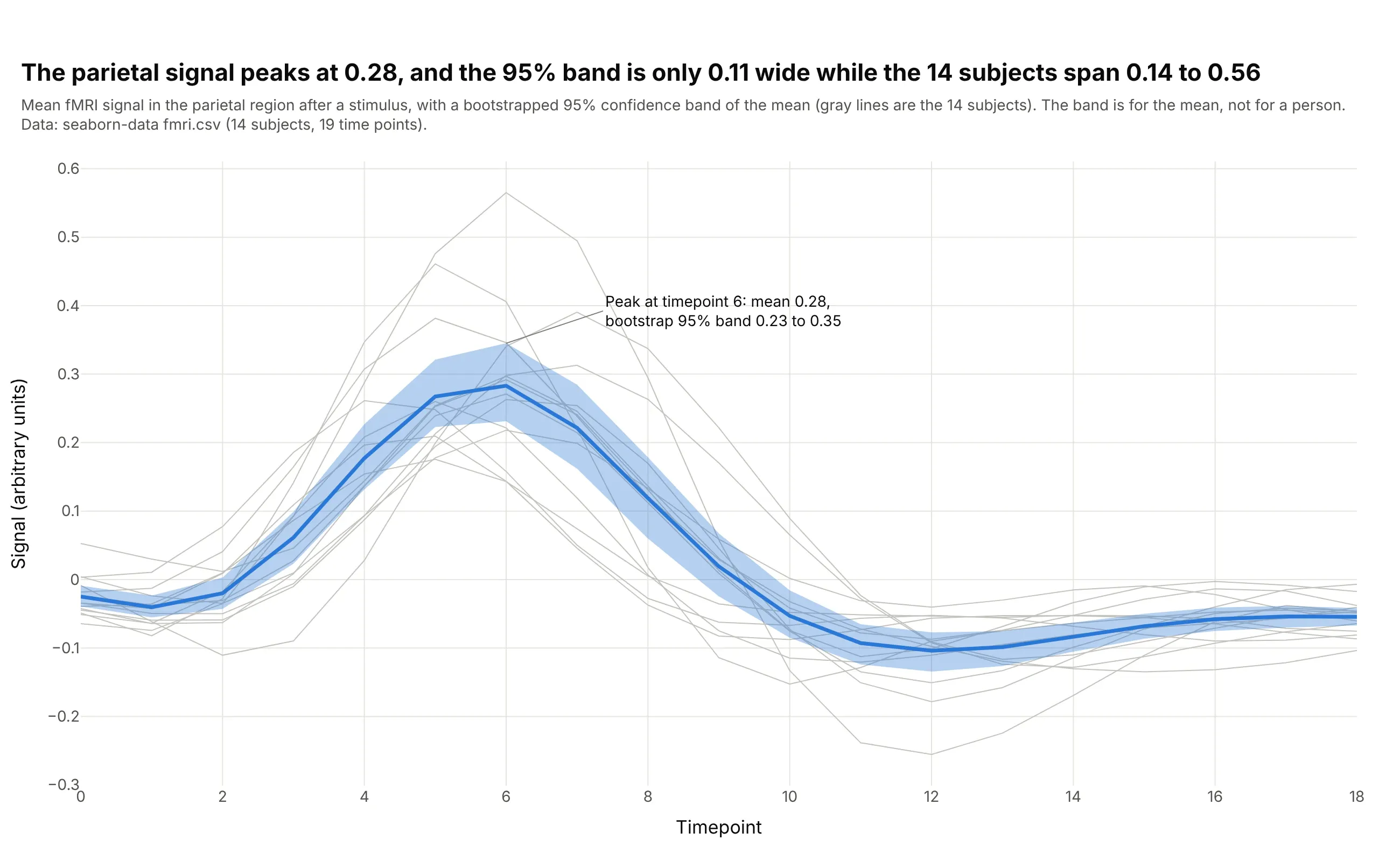
In seaborn's functional magnetic resonance imaging (fMRI) example data, 14 subjects were scanned for 19 time points after a stimulus. The mean parietal signal peaks at 0.28 at timepoint 6, and its bootstrapped 95% band is 0.23 to 0.35, which is 0.11 wide while the 14 subjects range from 0.14 to 0.56 at that point. The gray lines show why a confidence band is for the mean and not for a person. Data: seaborn-data fmri.csv (14 subjects, 19 time points, parietal region, stimulus event); the band is 2,000 bootstrap resamples at each time point with a fixed seed, and seaborn's own default is 1,000.
Tip: draw the individual subjects as thin gray lines behind the band, so the reader sees both the spread of the data and the narrower uncertainty of the mean.
Get the data from the seaborn-data repository (github.com/mwaskom/seaborn-data, file fmri.csv: subject, timepoint, event, region, signal).Build a plotly chart for region "parietal" and event "stim": draw each of the 14 subjects as a thin gray line, then the mean at each timepoint as a blue line with a 95% band from the 2.5th and 97.5th percentileof 2,000 bootstrap means (resampling the 14 values with replacement, seed 0), drawn with fill="toself". Annotate the peak with its mean and band.
4. A standard deviation band: Bollinger bands on the S&P 500
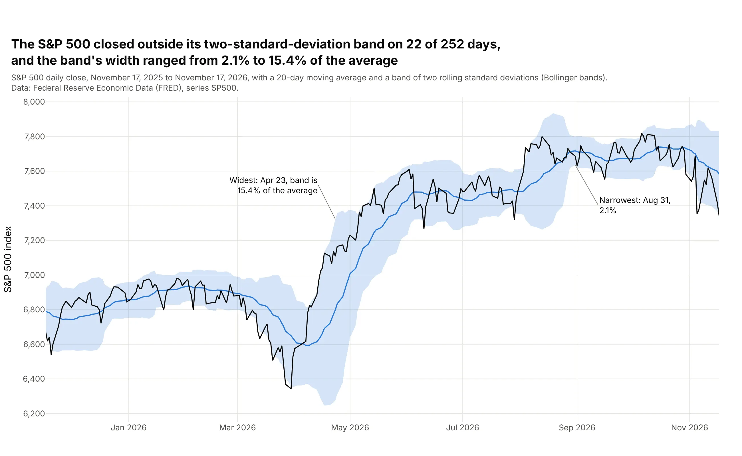
Bollinger bands put a 20-day moving average in the middle and a band two rolling standard deviations either side of it, so the band measures how much the price has been moving lately and nothing is being estimated. Over the past year the Standard & Poor's 500 (S&P 500) index of large US companies closed outside its band on 22 of 252 days (5 above and 17 below), and the band was 2.1% of the average wide on August 31 and 15.4% on April 23. Data: Federal Reserve Economic Data (FRED), series SP500, November 17, 2025 to November 17, 2026, with the standard deviation over 20 days computed as a population standard deviation (our calculation divides by 20).
Tip: state the window and the multiplier in the subtitle (20 days, two standard deviations), because the width of the band depends entirely on those two choices.
Get the data from the Federal Reserve Economic Data series SP500 (S&P 500 daily close, fred.stlouisfed.org/series/SP500) (columns: date, sp500).Build a plotly chart of the last 252 trading days: a 20-day rolling mean as a blue line, a band of plus and minus two rolling population standard deviations as a fill="toself" polygon,and the daily close in black. Count the days outside the band and annotate the widest and narrowest day (the band width divided by the average).
5. A band on a log scale: theophylline in the blood
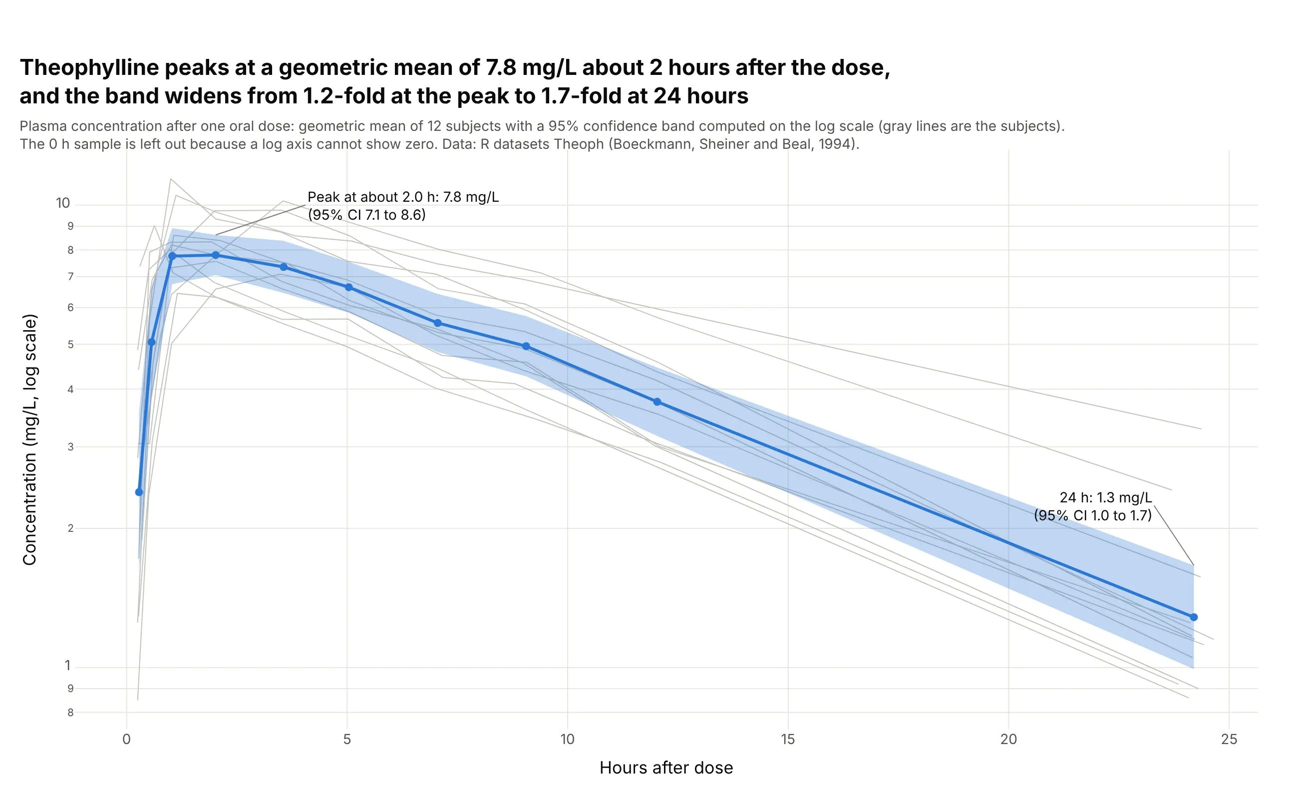
Drug concentrations are skewed and multiply from one sample to the next, so pharmacokinetics reports the geometric mean (the mean of the logarithms, converted back) with a confidence interval computed on the log scale. For 12 people given theophylline, an asthma drug, the geometric mean peaks at 7.8 mg/L about 2 hours after the dose (95% CI 7.1 to 8.6) and the band is 1.7-fold wide at 24 hours (1.0 to 1.7), against 1.2-fold at the peak. On a log axis the band is symmetric and it can never go below zero. Data: R datasets::Theoph (Boeckmann, Sheiner and Beal, 1994; a study by Dr. Robert Upton). The 0 h sample is left out because a log axis cannot show zero. See also the concentration-time curve guide.
Tip: compute the band on the logarithms and then exponentiate it, and set yaxis_type="log" so the band and the axis agree.
Get the data from the R datasets package, Theoph (Boeckmann, Sheiner and Beal, 1994: 12 subjects, theophylline concentration in mg/L over 24 hours after one oral dose)(columns: Subject, Wt, Dose, Time, conc).Build a plotly chart with a logarithmic y axis: group the samples by their position within each subject (the sampling times differ by minutes between subjects), drop the first sample, take the logarithm of conc,compute the mean and a t-based 95% interval at each position (12 subjects), exponentiate them back, and draw the geometric mean as a blue line with markers and the interval as a fill="toself" band over thin gray subject lines.
FAQ
Options to customize
A confidence band in Plotly is a filled scatter trace plus a line, so these are the options that matter most. The full lists are in the scatter trace reference, the filled area guide, the continuous error bars guide and the shapes guide.
- fill="tonexty": fills from a trace to the trace drawn before it, so an invisible upper line followed by a lower line with this option makes a band. It needs the traces in a strict order.
- fill="toself" with the x values forward and then backward: one closed polygon per band, which does not depend on trace order and is the better choice for several bands in one chart.
- fillcolor="rgba(42,120,214,0.25)": the band color with its opacity, usually the line color at 0.15 to 0.3 so the line stays the first thing the eye sees.
- line.width=0 and hoverinfo="skip": no outline on the band and no hover box on its edges, so the line carries the hover.
- showlegend=False on the edge traces, or legendgroup to link a band to its line: one legend entry per series instead of three.
- customdata and hovertemplate on the line: the band limits in the hover text, so one hover gives the value and its 95% range.
- error_y(type="data", symmetric=False, array=..., arrayminus=...): error bars at chosen x values, for the alternative that gives exact limits, and the same arguments exist in px.line as error_y and error_y_minus.
- scipy.stats.t.ppf(0.975, n - 1): the multiplier for a 95% interval of a mean, with the standard error s / sqrt(n); use scipy.stats.norm.ppf only for large samples or a known standard deviation.
- get_prediction(...).summary_frame(alpha=0.05): the confidence band (mean_ci_lower, mean_ci_upper) and the prediction band (obs_ci_lower, obs_ci_upper) of a fitted model in statsmodels.
- np.percentile(bootstrap_means, [2.5, 97.5]): a band that assumes no distribution, as in seaborn's lineplot and example 3.
- np.exp(...) on bands computed from logarithms with yaxis_type="log": bands that stay positive on skewed data, as in example 5.
- fig.add_hline(y=0), fig.add_vline(x=...) and fig.add_vrect(...): a reference line the reader compares with, a boundary between measured and forecast values and a shaded period.
- go.Scattergl: WebGL traces for line series with many points, with the caveat that a toself band of 100,000 x values failed in our test, so use the tonexty fill or the SVG trace for those bands.