Regression Plots - A Complete Guide

TL;DR

• A regression plot is a scatter plot with a fitted line or curve through it, usually an ordinary least squares (OLS) line, often with a shaded confidence band, so you can read how much y changes for each unit of x and how well that describes the points.
• Regression plots are also known as scatter plots with a trendline, regplots (after seaborn's regplot, with lmplot for several panels), fitted line plots and lines of best fit. They are similar to scatter plots, marginal plots, residual plots and binned scatter plots.
• Read the slope first (24% cheaper solar modules per doubling of installed capacity, 2.17 megawatts lost per degree of warmer air), then R², then the residuals, because four very different data sets can share one line (Anscombe's quartet).
• You can make one with Plotly in one line of code with px.scatter(df, x=..., y=..., trendline="ols"), switch to "lowess", "rolling", "ewm" or "expanding", and read the fitted model back with px.get_trendline_results.

What is a regression plot?

Regression plots look like this:

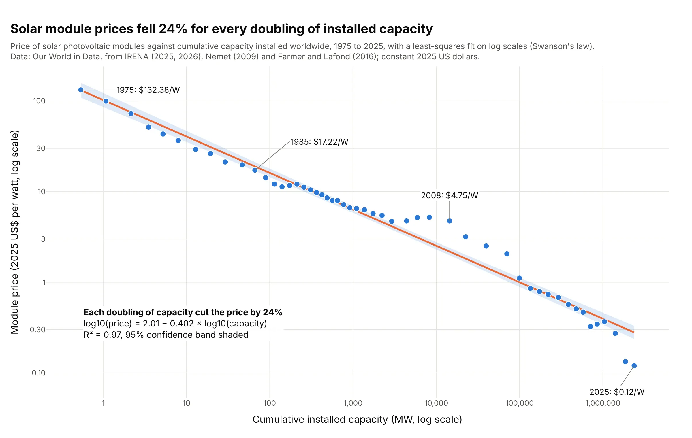
Data: Our World in Data, solar photovoltaic module prices (constant 2025 US dollars) and cumulative installed capacity, from the International Renewable Energy Agency (IRENA), Nemet (2009) and Farmer and Lafond (2016).

How do you read a regression plot? In the example above, notice these things:

• Each dot is one year from 1975 to 2025. Its x position is how many megawatts (MW) of solar panels the world had installed by then, and its y position is what a watt of module cost that year, both on log scales.
• The orange line is the least-squares fit to the logs. Its slope, −0.402, means that each doubling of installed capacity cut the price by 24% (1 − 2^−0.402), a pattern called Swanson's law.
• R² = 0.97 says the line accounts for 97% of the variation in the log price. The shaded band is the 95% confidence band for the line, and it's narrow because 51 points pin a straight line down well.
• The points the line misses tell their own story: from 2005 to 2011 prices sat well above it (2008 at $4.75 a watt, 2.2 times the fitted value), and by 2025 they were below it at $0.12, under half of the line's $0.28.

It's often used for charts like these:

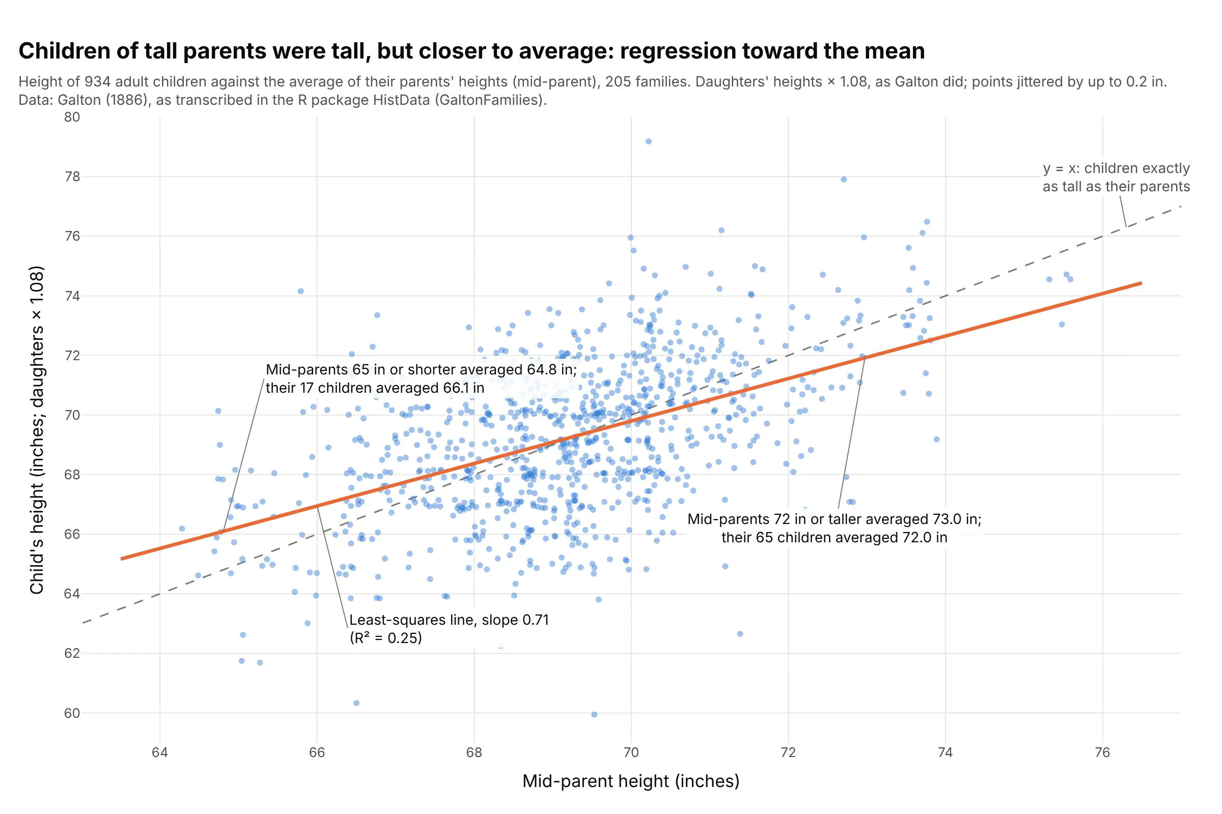
Heredity and regression toward the mean, the classic example. The least-squares line through Galton's 934 children has a slope of 0.71, flatter than the y = x line, so children of tall parents were tall but closer to average: mid-parents of 73.0 inches had children of 72.0. Data: Galton (1886), as transcribed in the R package HistData (GaltonFamilies).

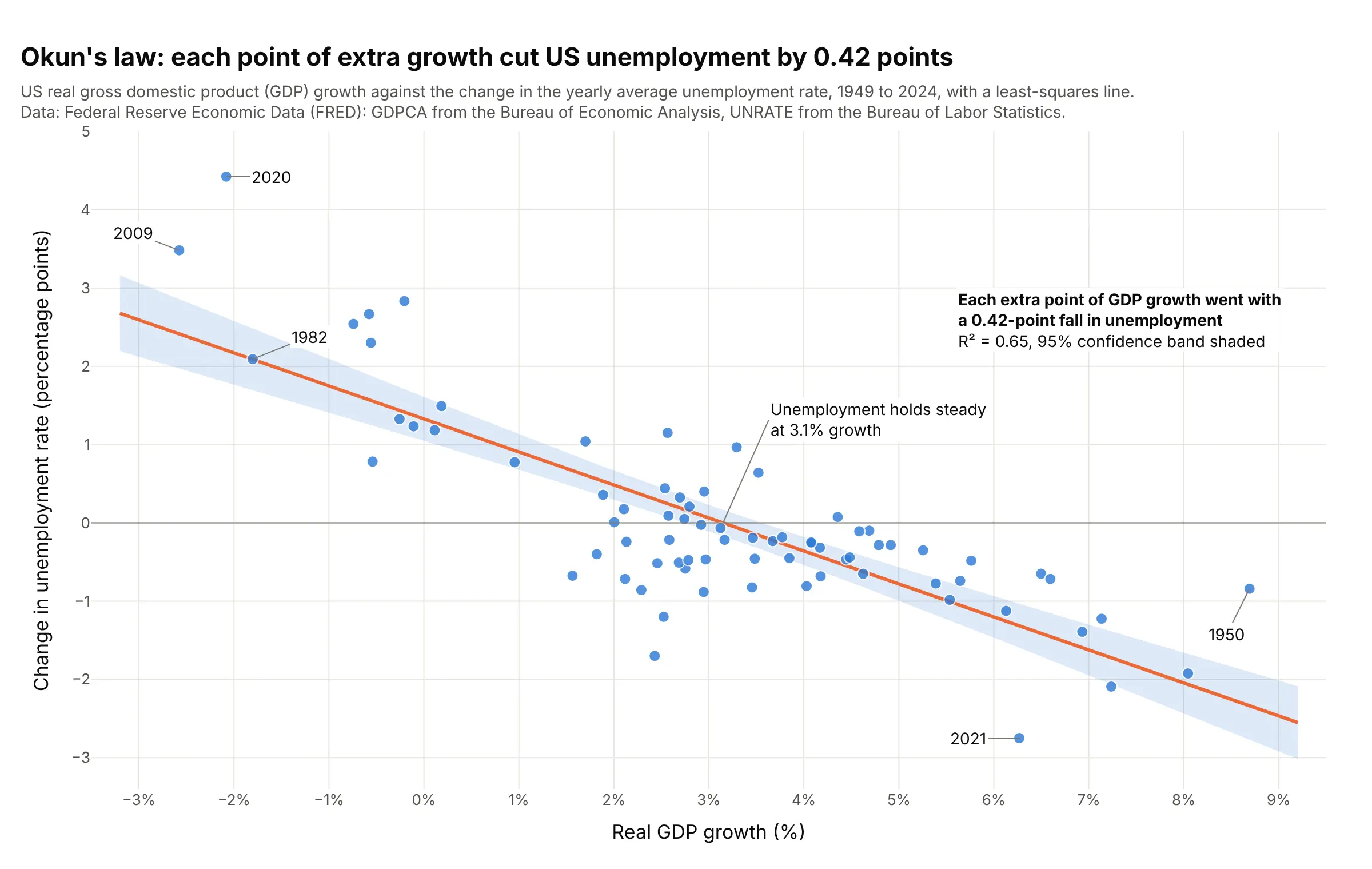
Economics and finance. Okun's law, the link between growth and jobs, is a regression line: each extra point of real gross domestic product (GDP) growth went with a 0.42-point fall in US unemployment from 1949 to 2024, and unemployment held steady at 3.1% growth. Data: Federal Reserve Economic Data (FRED), GDPCA from the Bureau of Economic Analysis and UNRATE from the Bureau of Labor Statistics.

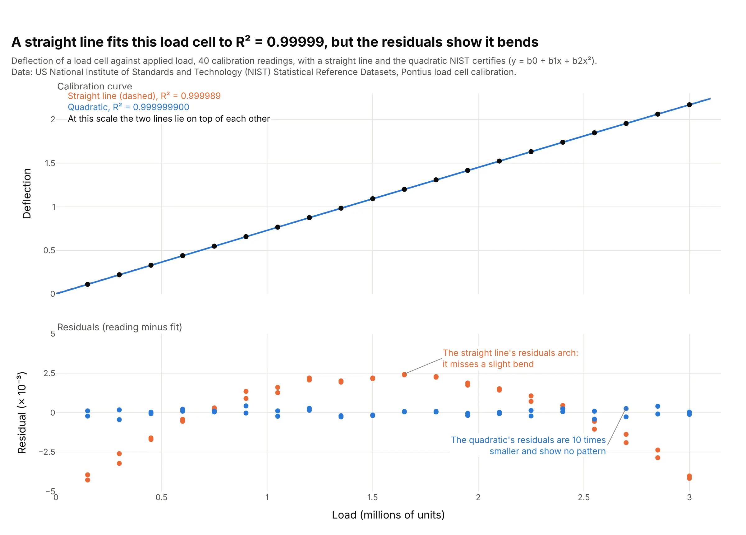
Calibration curves in labs and test benches. A straight line fits this load cell to R² = 0.99999, but its residuals arch, so the US National Institute of Standards and Technology (NIST) certifies a quadratic, whose residuals are 10 times smaller. Data: NIST Statistical Reference Datasets, Pontius load cell calibration.

How a regression line is fit

A regression plot answers one question: if x goes up by one unit, how much does y go up or down on average? The line is the answer, and the rest of the chart (the band, R², the residuals) tells you how far to trust it. These four ideas are all you need to read one, and each is shown on real data below.

Least squares: the line with the smallest squared misses

For any straight line, each point has a residual, its vertical distance from the line (observed y minus the line's y at that x). Ordinary least squares picks the one line that makes the sum of the squared residuals as small as possible. Squaring makes misses above and below the line count the same and punishes big misses more than small ones:

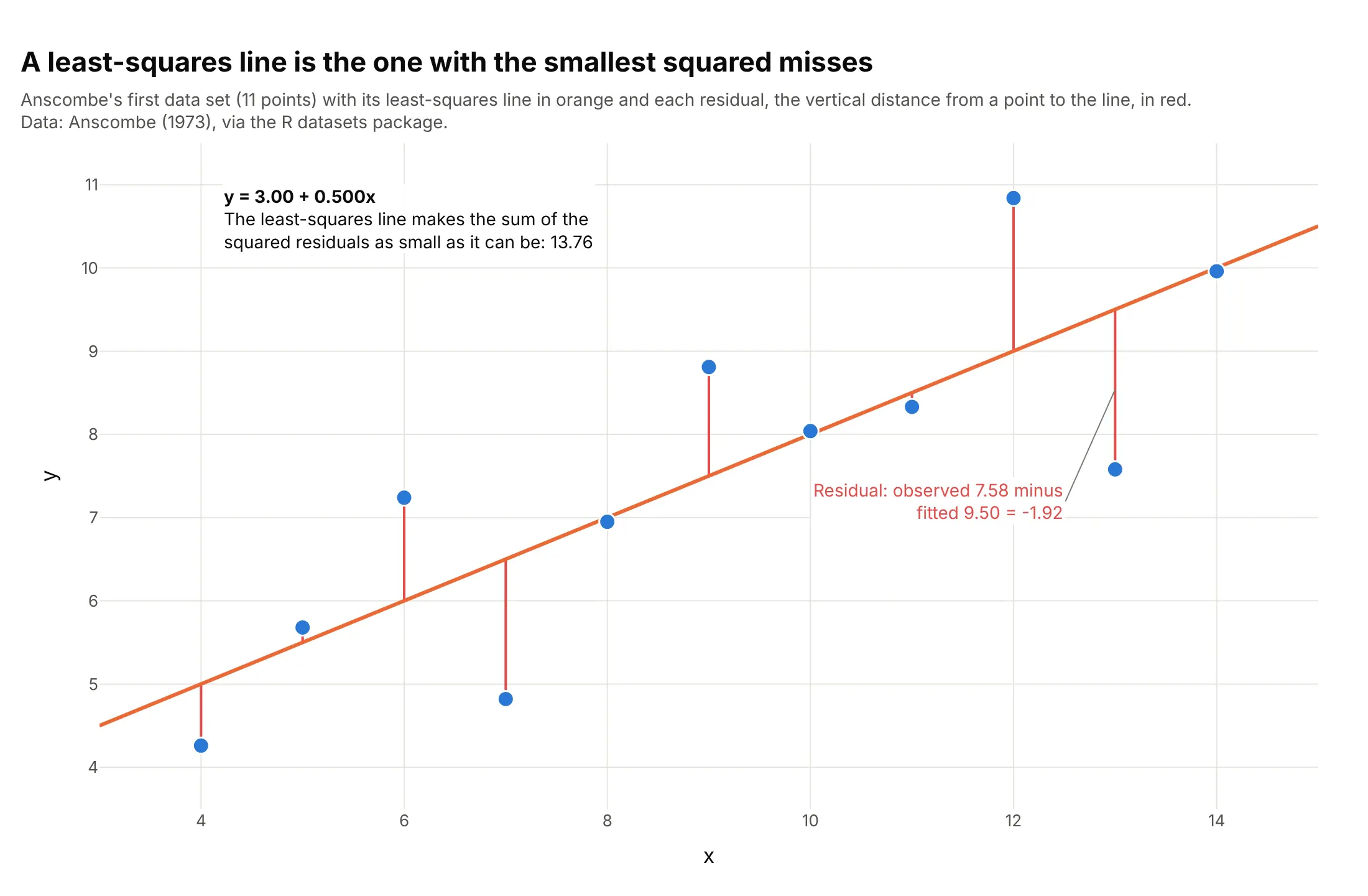
Data: Anscombe (1973), via the R datasets package.

For a straight line the answer has a short formula: the slope is the covariance of x and y divided by the variance of x, and the line passes through the point (mean of x, mean of y). Here that gives y = 3.00 + 0.500x, and no other straight line has a smaller sum of squared residuals than 13.76. Because squares grow fast, one point far from the others can pull the line toward it, which is why you look at the plot before you trust the numbers.

R²: how much of the spread the line explains

R² (R-squared, the coefficient of determination) compares two totals. The first is the sum of squared distances from each point to the mean of y, the spread you would have with no line at all. The second is the sum of squared residuals the line leaves over:

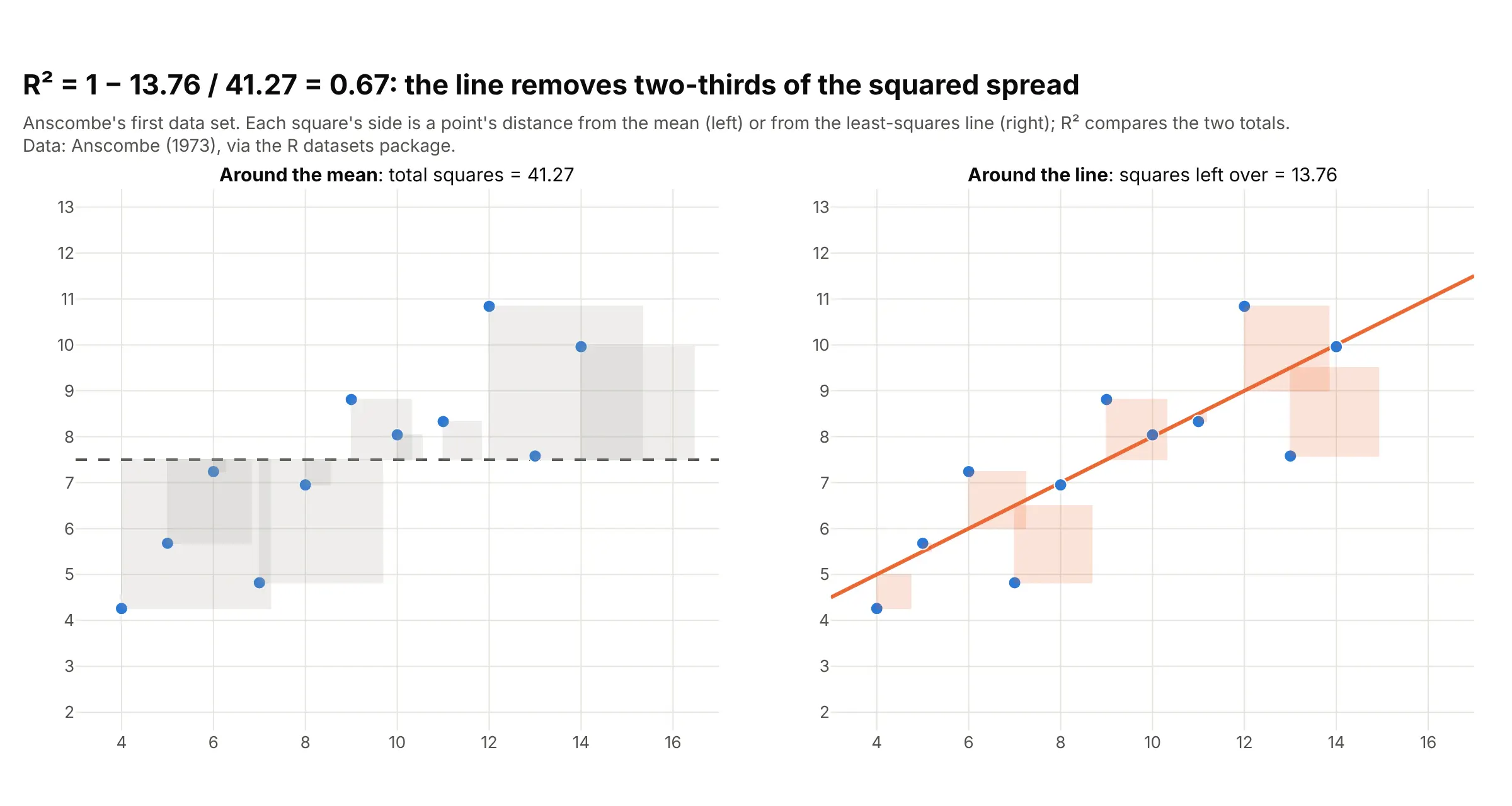
Data: Anscombe (1973), via the R datasets package.

R² is 1 minus the second total divided by the first: 1 − 13.76 / 41.27 = 0.67, so the line removes two-thirds of the squared spread. R² runs from 0 (the line does no better than the mean) to 1 (every point is on the line). What counts as high depends on the field: 0.25 for Galton's heights is normal for people, where much of the variation is individual, while a calibration curve below 0.999 would be a problem. A high R² doesn't mean a straight line is the right shape, as the load cell and Anscombe's quartet below show.

Confidence band and prediction band

The shaded band around a regression line is usually a 95% confidence band: if you collected new data the same way many times, the true line would fall inside the band 95% of the time. A prediction band is wider, because it adds the scatter of single points around the line, and it answers a different question, where the next observation is likely to land:

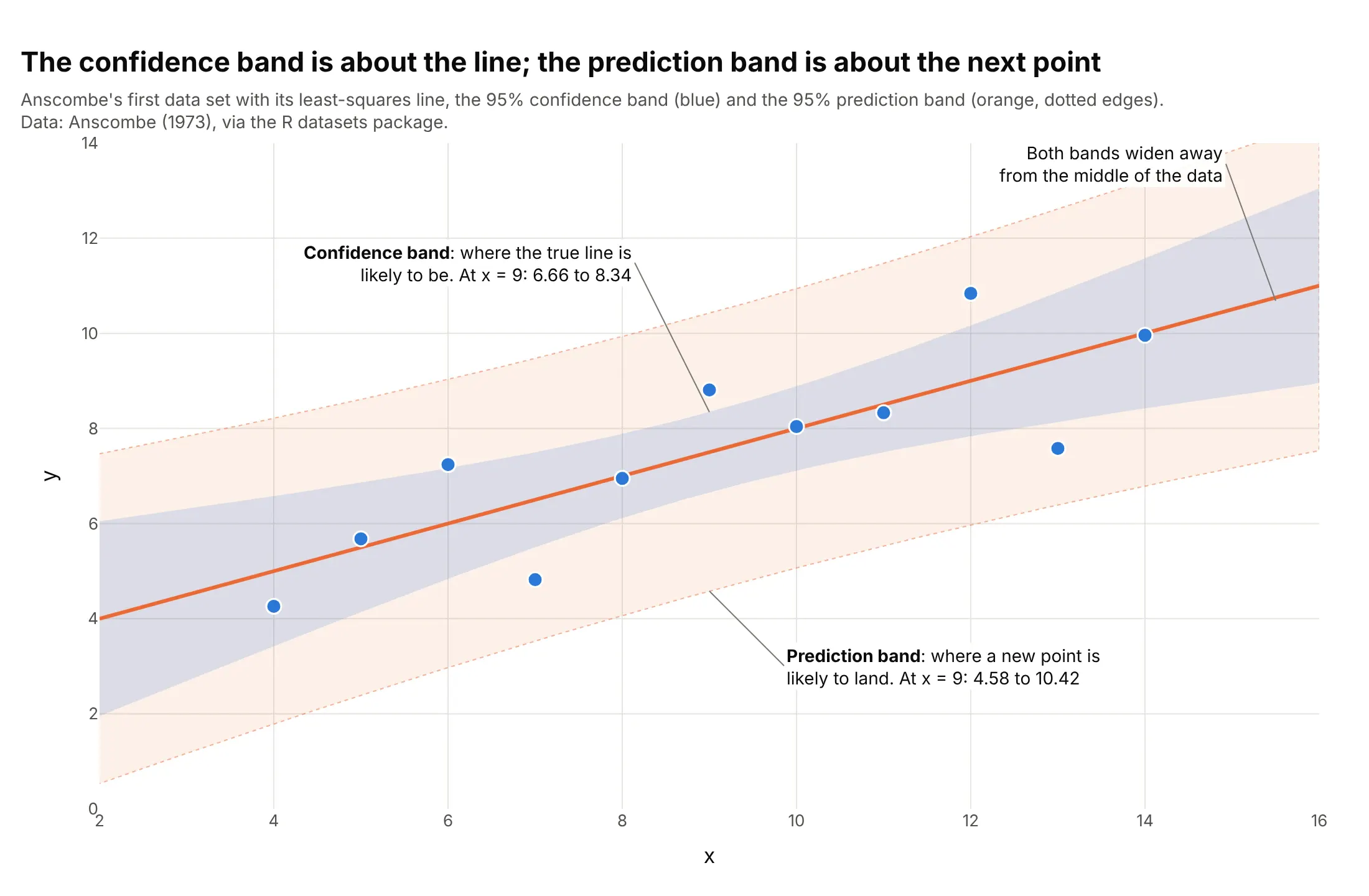
Data: Anscombe (1973), via the R datasets package.

At x = 9, the middle of the data, the line is pinned between 6.66 and 8.34, but a new point could land anywhere from 4.58 to 10.42. Both bands are narrowest at the mean of x and widen toward the ends, because a small change in the slope moves the line most far from the middle. With more points the confidence band shrinks toward the line, while the prediction band never gets narrower than the scatter itself. Use the confidence band to say how well you know the slope, and the prediction band to say how far a single season, batch or patient can stray, as in the baseball example below.

Residual plots: what the line missed

A residual plot draws the residuals against x (or against time, or against the fitted values) with a line at zero. If the model has the right shape, the residuals form a flat band with no pattern. A curve means the shape is wrong, and a funnel means the spread changes with x:

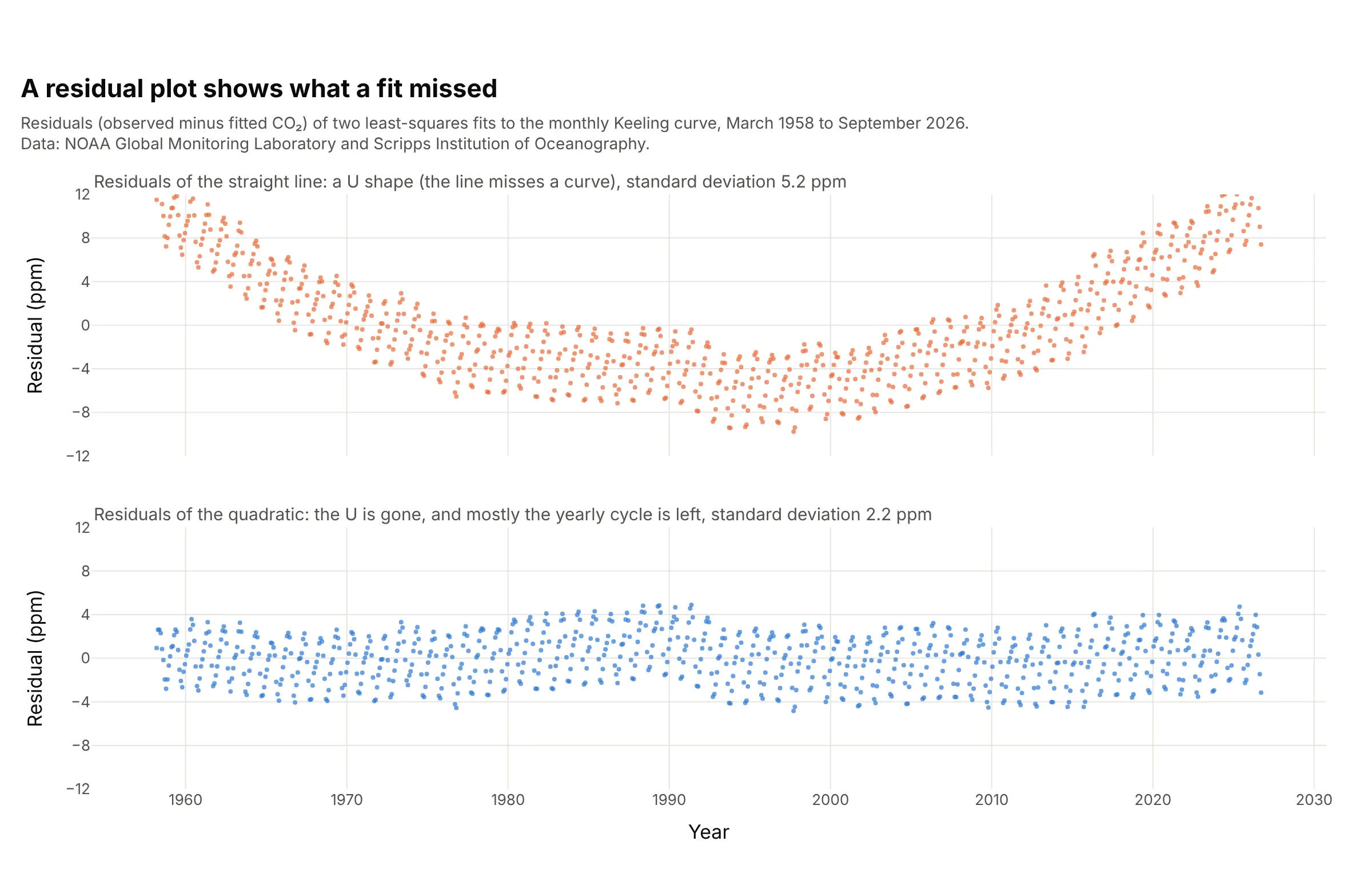
Data: NOAA Global Monitoring Laboratory and Scripps Institution of Oceanography, monthly mean carbon dioxide (CO₂) at Mauna Loa.

A straight line through 68 years of CO₂ readings has an R² of 0.975, which sounds excellent, but its residuals form a U: the line is too high in the middle and too low at both ends, because CO₂ is rising faster each decade. A quadratic, a curve with one bend, removes the U and leaves mostly the yearly cycle of plants growing and decaying, with a residual standard deviation of 2.2 parts per million (ppm) instead of 5.2. To check whether the residuals also follow a normal distribution, the assumption behind the bands, draw them on a Q-Q plot.

A short history

Adrien-Marie Legendre published the method of least squares in 1805, fitting the shape of the Earth from survey measurements, and Carl Friedrich Gauss used it for planetary orbits in 1809 (Wikipedia: Least squares). The word regression comes from Francis Galton's 1886 paper Regression towards mediocrity in hereditary stature, the heights shown above, where the fitted line was flatter than y = x. William Cleveland's LOWESS paper (1979) gave the smooth curve most tools draw today. The best-known argument for drawing the plot instead of reporting only the numbers is Francis Anscombe's 1973 quartet, redrawn here from his published values:

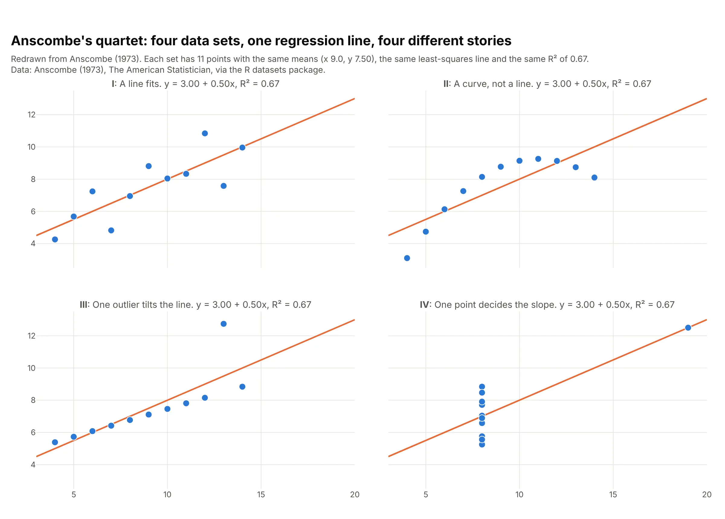
Data: Anscombe (1973), The American Statistician, via the R datasets package.

All four sets have the same means, the same least-squares line, y = 3.00 + 0.50x, and the same R² of 0.67, but only the first is described well by that line. The second needs a curve, the third has one outlier tilting the line, and in the fourth a single point decides the slope.

Alternatives to a regression plot

Here's the same 9,568 hours of a gas-fired power plant drawn six ways. Some are better for the question, some worse, some just different:

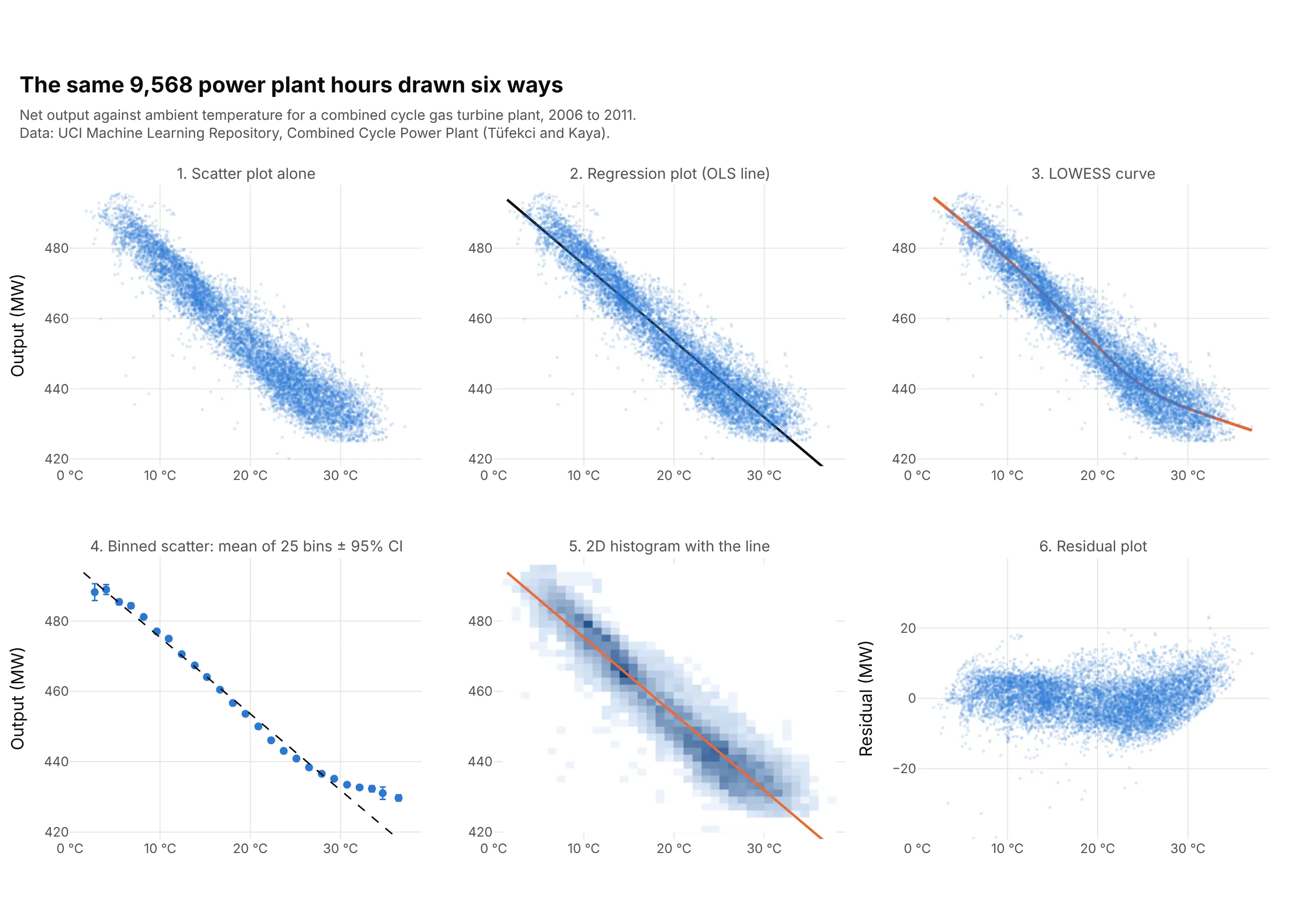
• Scatter plot alone (worse for the slope, works too for a first look). It shows the shape and the outliers, but readers have to guess the slope by eye, and with 9,568 points the dense middle hides how many points are where.
• LOWESS curve (better when the shape isn't a straight line). Locally weighted scatterplot smoothing (LOWESS) follows the data without assuming a shape. Here it shows output falling about 2.3 MW per degree up to 25 °C and only 1.1 above it, which the straight line misses. It gives no single slope to report.
• Binned scatter plot (better for big data and for showing curvature). Averaging y in 25 bins of x, with error bars, turns thousands of points into a few means you can read exactly, and it makes the flattening above 30 °C obvious. You lose the individual points and the outliers.
• 2D histogram or hexbin plot with the line (better for overplotting). Counting points per cell shows where most hours are, which a cloud of transparent dots only hints at.
• Residual plot (different, and the one to draw next). It removes the trend so you can see what's left: here the residuals sag between about 18 and 27 °C and climb above 30 °C, so a curve would fit better than a line.
• Marginal plot (works too). A histogram on each edge of a regression plot adds the distribution of each variable, like seaborn's jointplot(kind="reg").

How to make a regression plot

With AI

ChatGPT, Claude Code, GitHub Copilot, Cursor and other AI tools are excellent at writing Plotly code. Name Plotly in the prompt, and say which kind of fit you want, whether to transform the axes and which numbers from the fit to show:

With Plotly Studio

Plotly Studio is a desktop app where you point an AI at a dataset and it builds charts and a Dash app around your questions. Ask for a regression plot the same way:

Show net electrical output against ambient temperature as a regression plot with an OLS trendline and its slope in MW per °C, a dropdown to switch the trendline between OLS, LOWESS and a rolling mean, and a residual plot underneath.

Make a regression plot in Python or JavaScript

This is the code AI tools write under the hood. In Python, Plotly Express adds a fitted line to a scatter plot with the trendline argument and fits it with statsmodels, so you need pip install plotly statsmodels. The trendline documentation covers every option:

px.get_trendline_results(fig) returns a table with one fitted model per trace, so with color= or facets you get one row per group. The same argument draws five other kinds of trendline, shown here on the monthly CO₂ record:

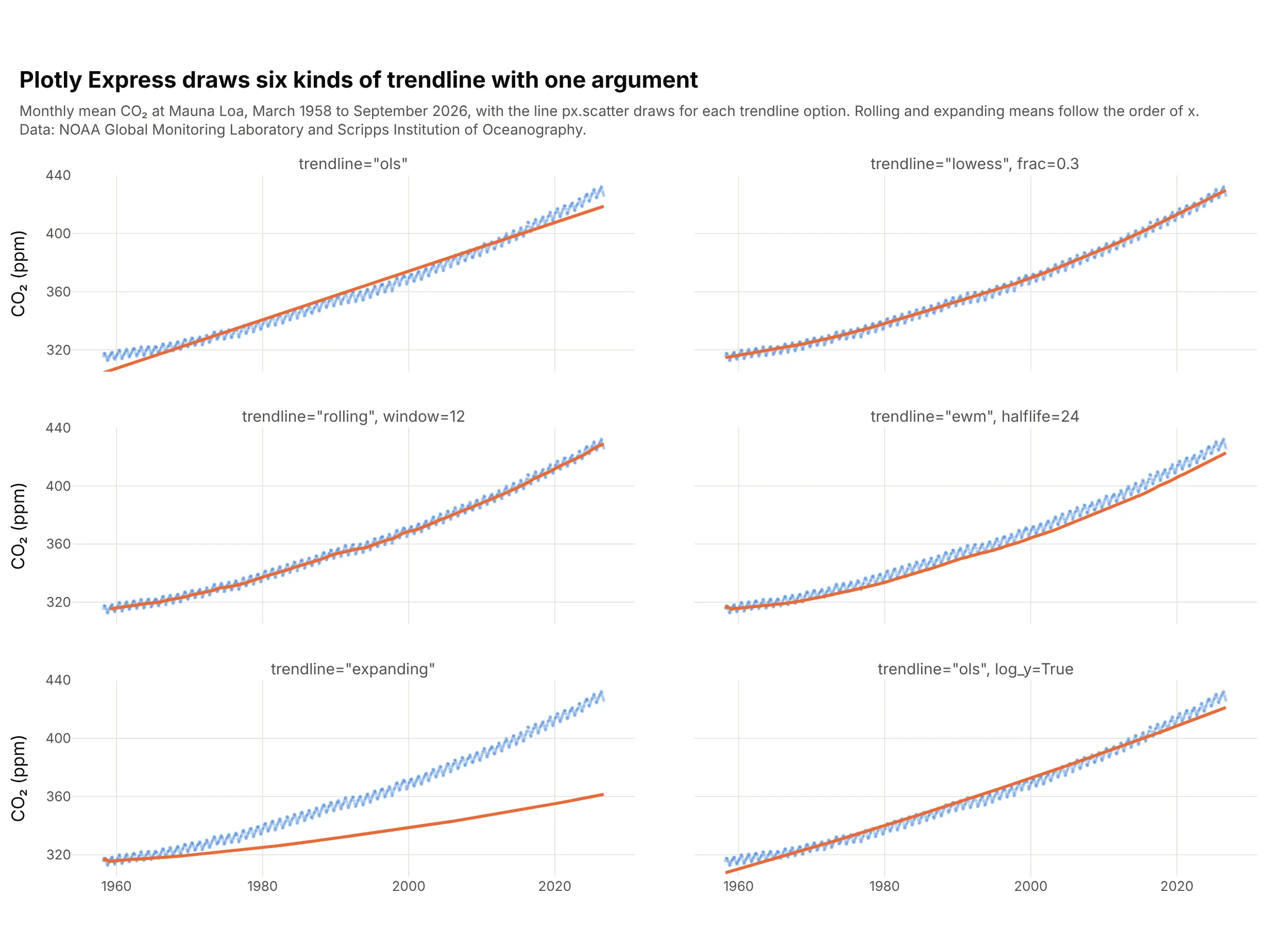
Data: NOAA Global Monitoring Laboratory and Scripps Institution of Oceanography.

"rolling" is a moving average over a window of points, "ewm" is an exponentially weighted moving average (EWM) that gives recent points more weight, and "expanding" is the running average of every point so far, which lags behind any trend and suits a stable process better. These three follow the order of the rows, so sort by x first.

Plotly Express doesn't shade a confidence band the way seaborn's regplot does, but statsmodels computes both bands and Plotly draws them as a filled trace, which also lets you choose the confidence level:

For a residual plot, fit the model with statsmodels' formula interface, which also handles curves such as I(x**2), and plot model.resid:

In JavaScript, plotly.js draws a regression plot from a markers trace and a lines trace once you've computed the least-squares line, which takes a few lines:

Share it

Every Plotly chart has a Share chart button (the cloud icon in its toolbar) that uploads it to Plotly Cloud and gives you a link. Only you can see it until you change its visibility.

For a live app, put the chart in a Dash app and publish it with the Plotly Cloud command-line interface (CLI). Coding agents can run these commands for you:

If your data has to stay in your own cloud or data center, publish to Dash Enterprise instead.

Dos and don'ts

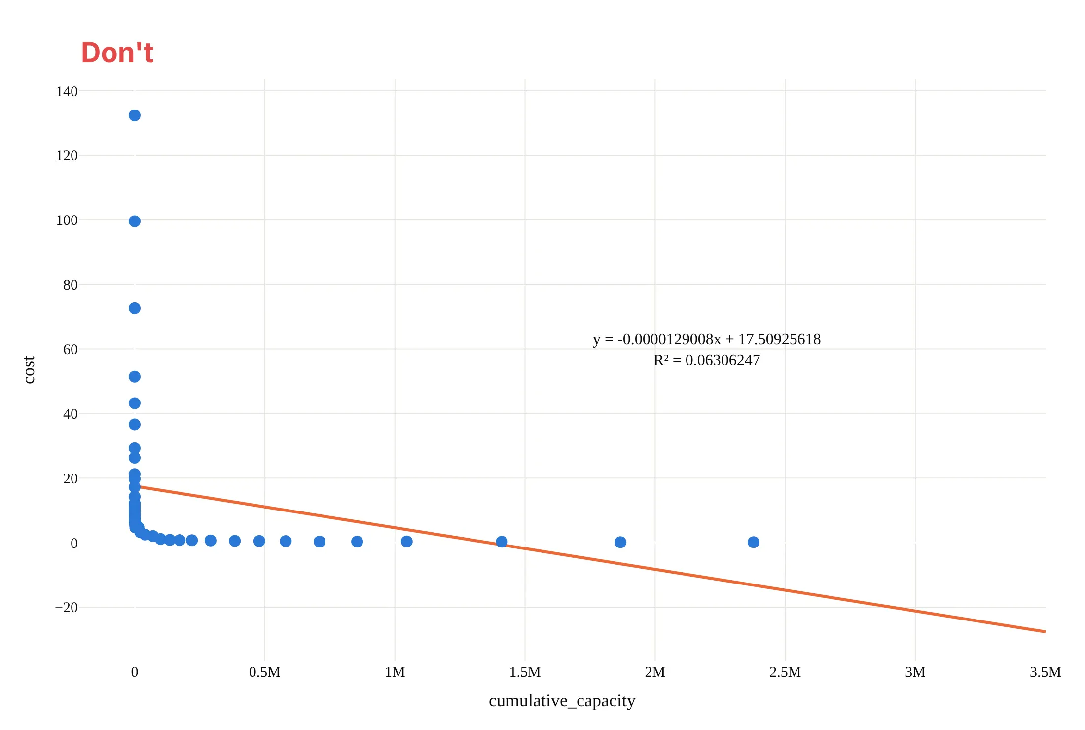
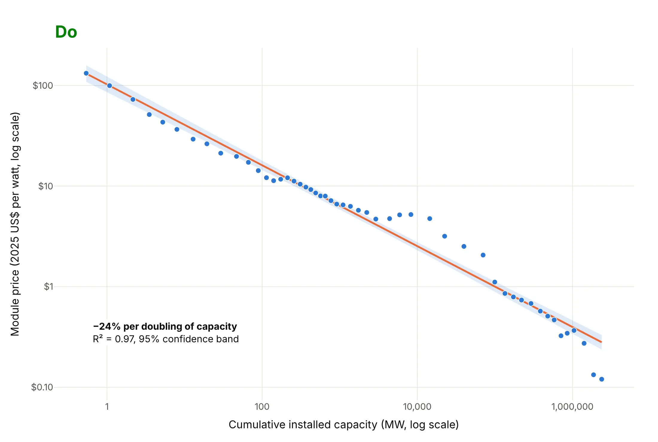
Most regression plot mistakes are about the model rather than the styling: fitting a straight line to data that isn't straight, drawing it past the data and reporting more digits than the data support. Here is the solar price data both ways, in the same colors.

Don't fit a straight line to raw values that span six orders of magnitude, extend it past the data until it predicts negative prices, print an unrounded equation and an R² of 0.06306247, keep the raw column names as axis titles or use a default serif font:

Do transform the axes until the relationship is straight (here log-log, the scale learning curves live on), fit the line on that scale, keep it within the range of the data, add a confidence band, write axis titles with units and state the fit in words:

Checklist

Do

• Plot the data before you trust the fit, and draw a residual plot when the shape matters.
• Use log axes and fit on the logs (trendline_options=dict(log_x=True, log_y=True)) for data that grows by multiples, like prices, sizes and doses.
• Say what kind of fit it is (OLS, LOWESS, a 12-month rolling mean) and what the band is (a 95% confidence or prediction band).
• Report the slope in the units readers care about (MW per °C, runs per win, % per doubling), rounded.
• Use trendline_scope="overall" or one line per group on purpose, and check whether the groups disagree.
• Use WebGL (render_mode="webgl") and low marker opacity above about 10,000 points.

Don't

• Extend the line far beyond the data; the fit says nothing about what happens there.
• Read a high R² as proof that a straight line is the right shape.
• Report R² without the slope, or a slope without its units.
• Fit one line through groups that behave differently (see the penguins example).
• Treat a regression line as cause and effect; it describes how y moves with x in this data.

Options to customize

A regression plot in Plotly is a scatter trace plus a fitted line from Plotly Express or from statsmodels, so these are the options that matter most. The full lists are in the trendline documentation, the px.scatter reference and the statsmodels regression documentation.

1. trendline: "ols" for a least-squares line, "lowess" for a smooth local fit, "rolling", "ewm" or "expanding" for moving averages.
2. trendline_options: frac for LOWESS (smaller follows the points more closely), window, halflife and other pandas arguments for the moving averages, log_x, log_y and add_constant for OLS.
3. trendline_scope: "trace" (the default) fits one line per color, symbol or facet; "overall" fits one line to all the points.
4. trendline_color_override: one color for every trendline, such as black over colored points.
5. px.get_trendline_results(fig): a table of fitted statsmodels results, one per trace, with params, rsquared, conf_int() and summary().
6. log_x, log_y: log axes, usually together with the matching trendline_options so the fit is straight on screen.
7. render_mode="webgl" and opacity: fast drawing and readable density for tens of thousands of points or more.
8. facet_col, facet_row: one panel per group with its own line, like seaborn's lmplot.
9. marginal_x, marginal_y: histograms, box plots or rugs on the edges.
10. model.get_prediction(X).summary_frame(alpha=0.05) (statsmodels): the confidence band (mean_ci_*) and prediction band (obs_ci_*) for any fitted model.
11. fill="toself" or fill="tonexty": a shaded band from the lower and upper edges.
12. smf.ols("y ~ x + np.square(x)", data=df) (statsmodels formula interface): curved and multi-variable fits, with model.resid for the residual plot.

More regression plot examples

Six more regression plots built from real public data, each with its source, the technique that makes it work and a prompt to rebuild it.

1. The Keeling curve with a curved fit

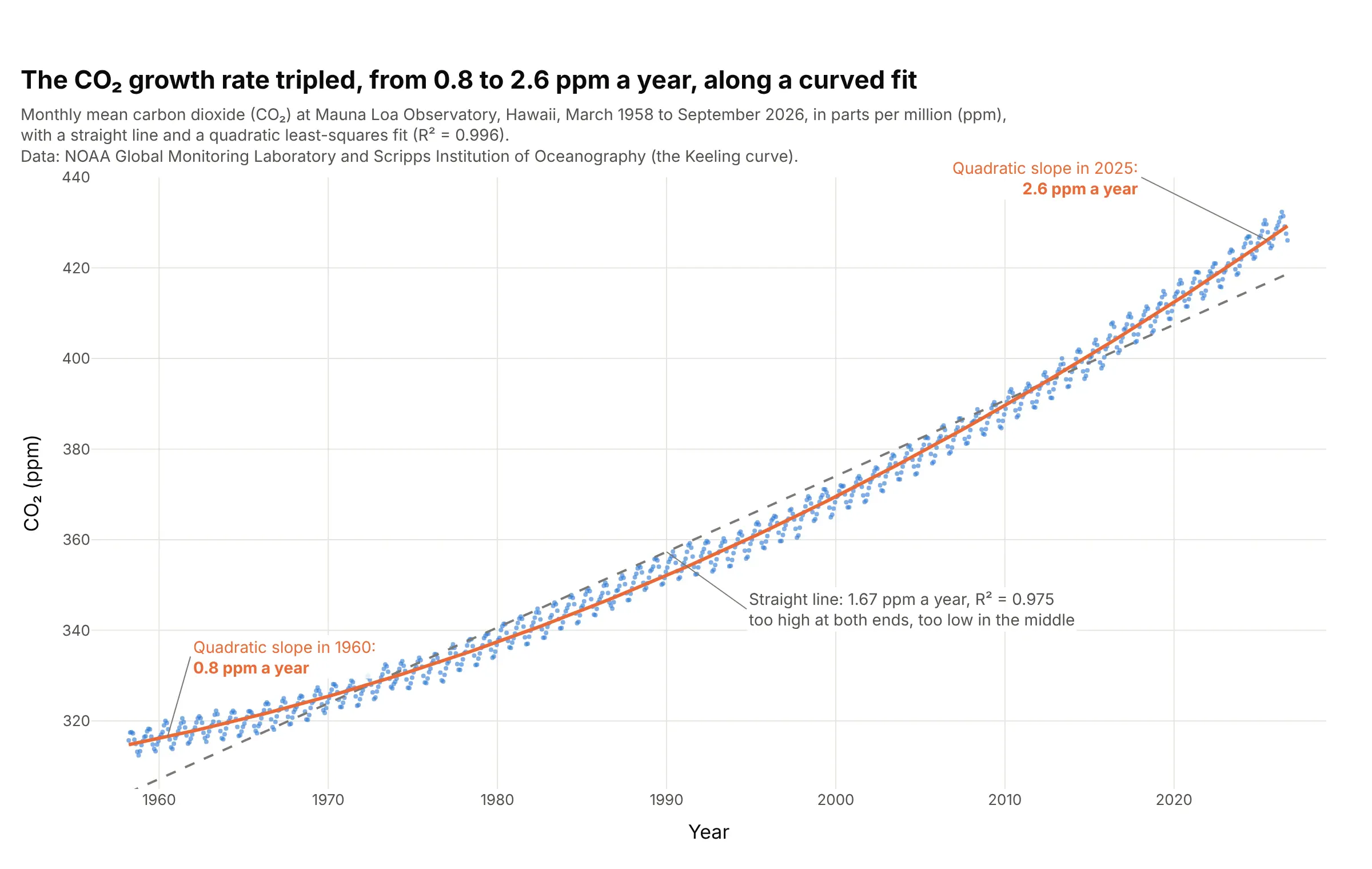
A straight line through 823 monthly CO₂ readings gives 1.67 ppm a year, but a quadratic fits better (R² 0.996) and its slope shows the growth rate itself rising, from 0.8 ppm a year in 1960 to 2.6 in 2025. Data: NOAA Global Monitoring Laboratory and Scripps Institution of Oceanography, Mauna Loa monthly mean CO₂.

Tip: the slope of a quadratic at time t is b1 + 2·b2·t, so label the curve with its slope at a few dates instead of printing the coefficients.

2. A power plant loses 2.17 MW for every degree of warmer air

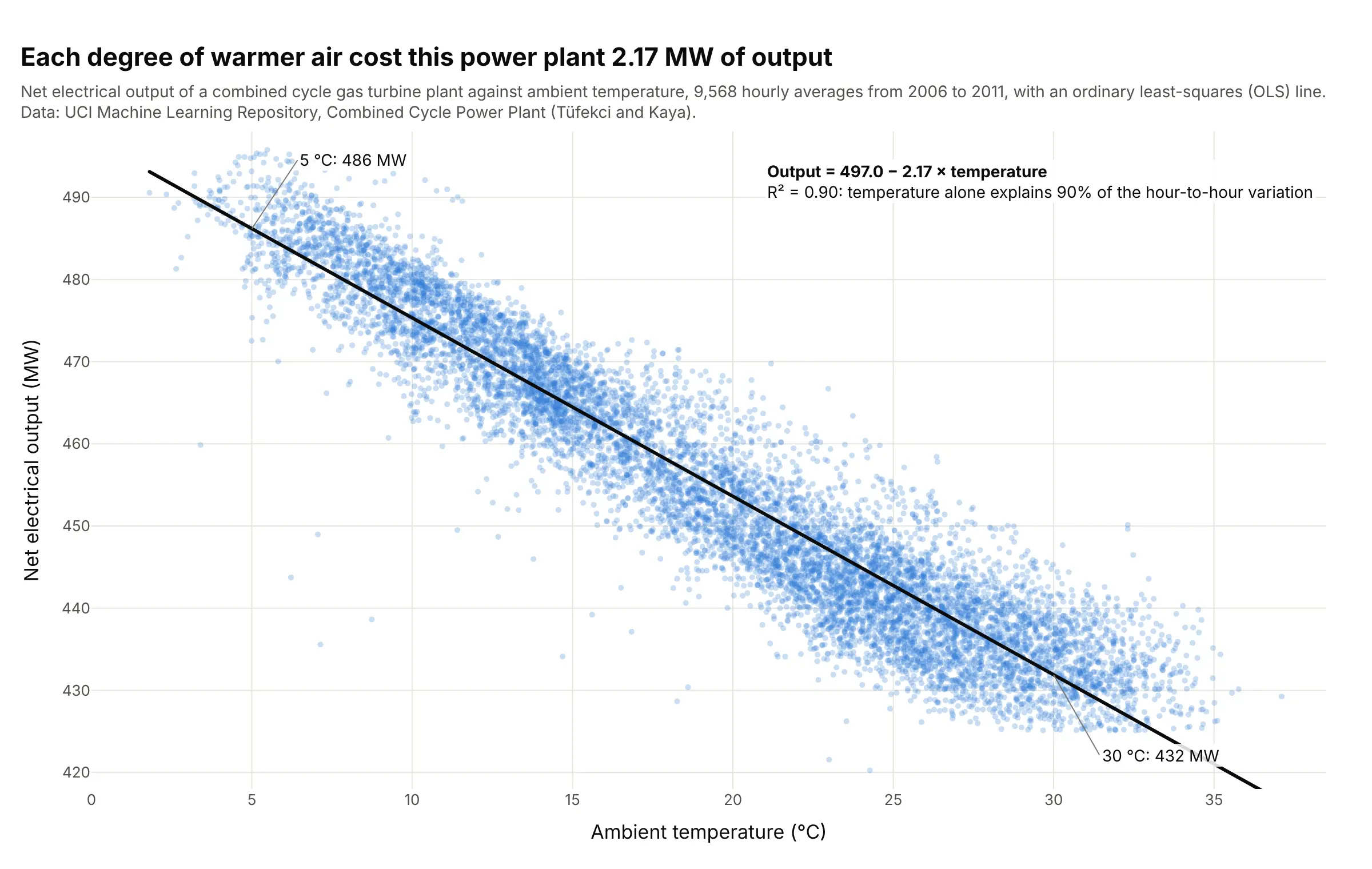
Warm air is less dense, so a gas turbine burns less of it, and across 9,568 hours this plant's output fell 2.17 MW for each degree, from 486 MW at 5 °C to 432 MW at 30 °C. Temperature alone explains 90% of the variation (R² 0.90). Data: UCI Machine Learning Repository, Combined Cycle Power Plant (creators Pınar Tüfekci and Heysem Kaya; described in Tüfekci, 2014).

Tip: with thousands of points use render_mode="webgl", opacity=0.25 and a black trendline_color_override, so the line stays visible over the cloud.

3. Penguins: one line for all species slopes the wrong way

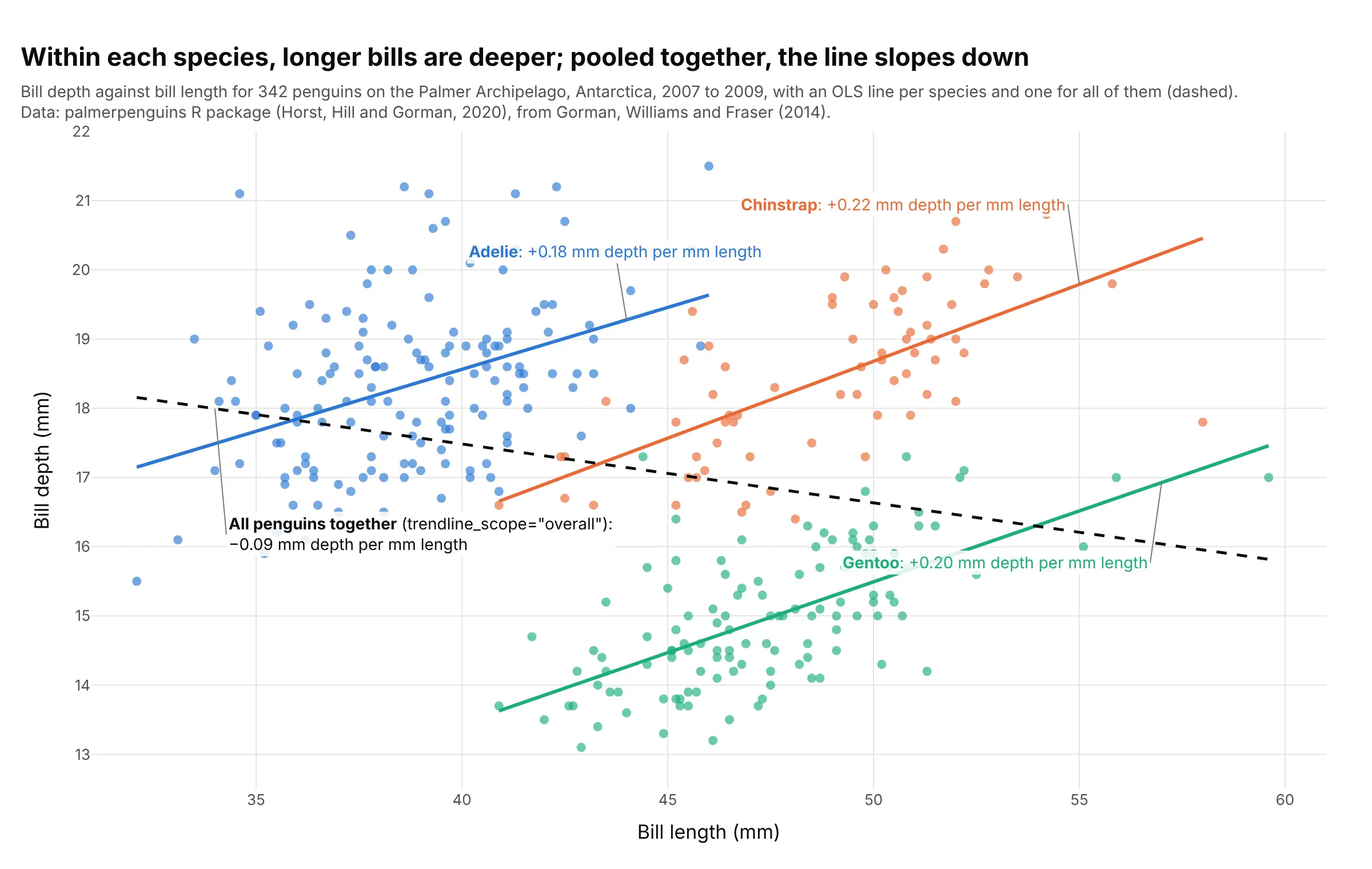
Within each species, a penguin with a longer bill has a deeper one (+0.18 to +0.22 mm per mm), but one line through all 342 birds slopes down (−0.09), because Gentoo penguins have long, shallow bills. This reversal is called Simpson's paradox. Data: palmerpenguins R package, from Gorman, Williams and Fraser (2014).

Tip: draw the per-group lines with color= and add the trendline_scope="overall" line dashed, so readers see both answers at once.

4. Kleiber's law: metabolic rate against body mass

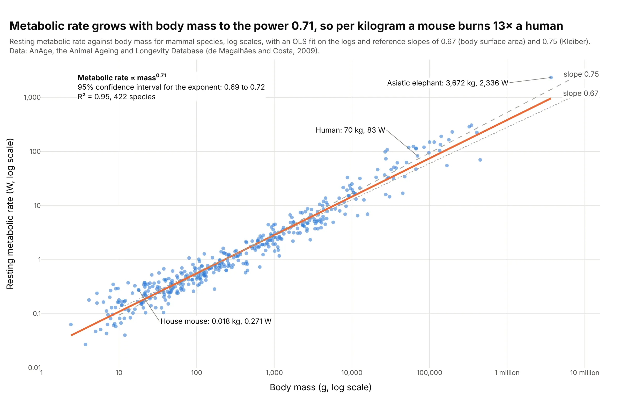
Across 422 mammals, metabolic rate grows with body mass to the power 0.71 (95% confidence interval 0.69 to 0.72), so per kilogram a mouse burns 13 times what a person does. The same scaling is why drug doses don't carry over from animals to people by weight: the US Food and Drug Administration's (FDA) first-in-human dose guidance converts by body surface area, mass to the power 0.67. Data: AnAge, the Animal Ageing and Longevity Database (de Magalhães and Costa, 2009).

Tip: trendline_options=dict(log_x=True, log_y=True) fits a power law, and its slope is the exponent, so add the textbook exponents as dashed reference lines to compare.

5. Blood pressure by age with LOWESS trendlines

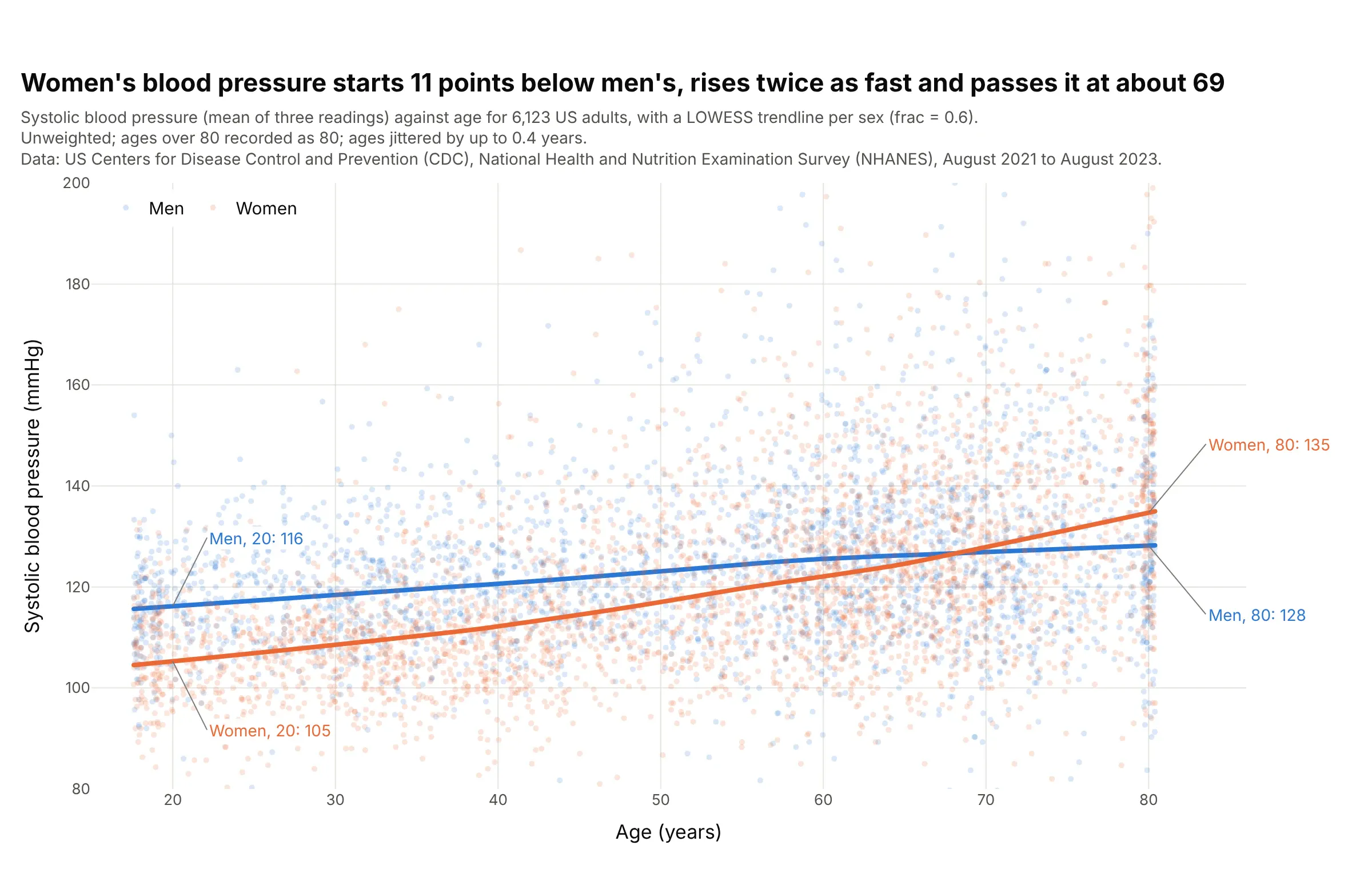
Women's systolic blood pressure starts about 11 points lower than men's at 20, rises twice as fast with age and passes it at about 69. LOWESS shows that bend without assuming a shape. Data: US Centers for Disease Control and Prevention (CDC), National Health and Nutrition Examination Survey (NHANES), August 2021 to August 2023, unweighted.

Tip: whole-number ages stack into columns, so add a small random jitter to x for display and say so in the subtitle.

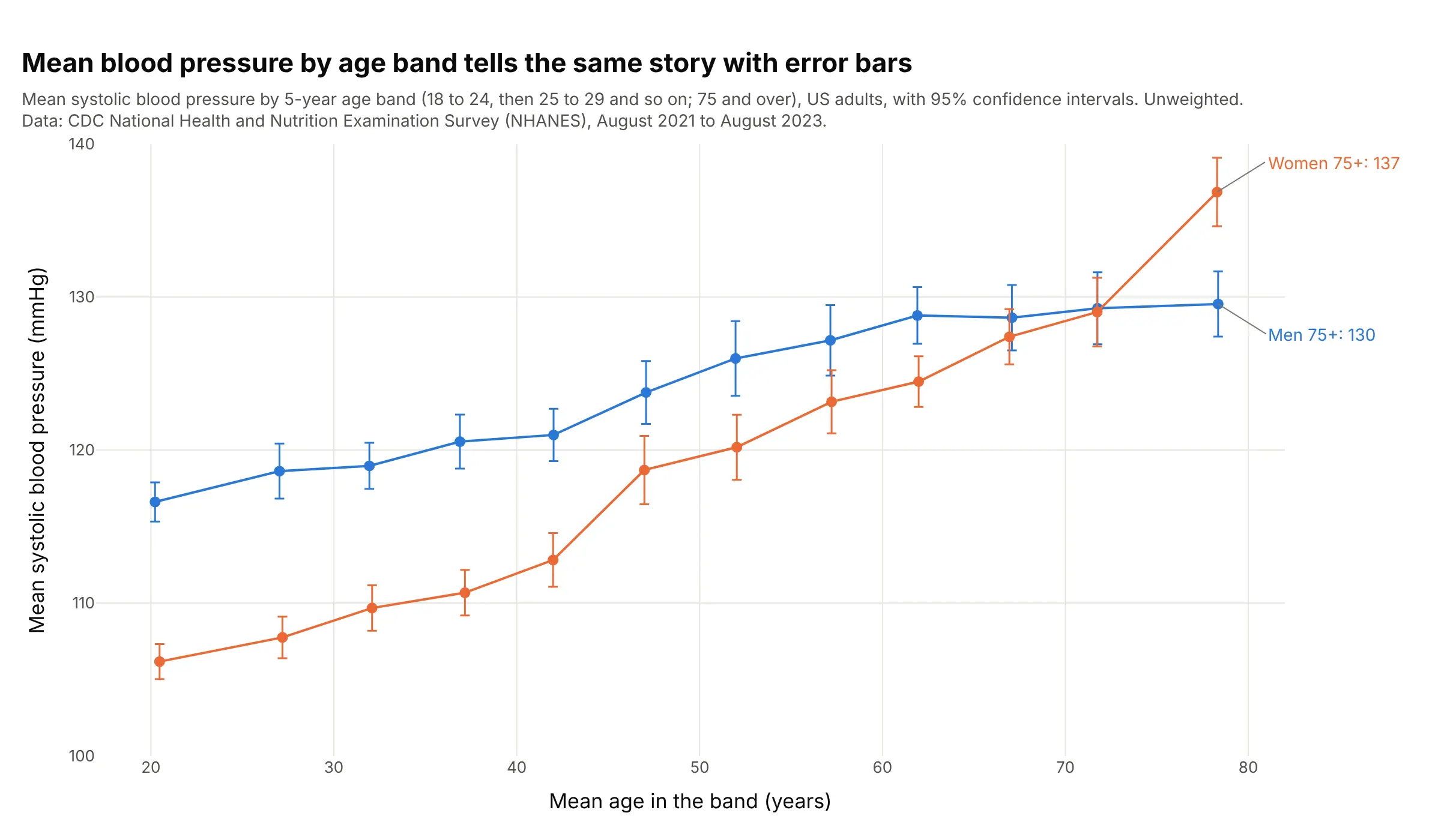
Another way to see it: a binned scatter plot, the mean of each 5-year age band with its 95% confidence interval, shows the same crossing with error bars, and shows women's average rising fastest between the early 40s and the late 40s:

6. Runs and wins in Major League Baseball, with a prediction band

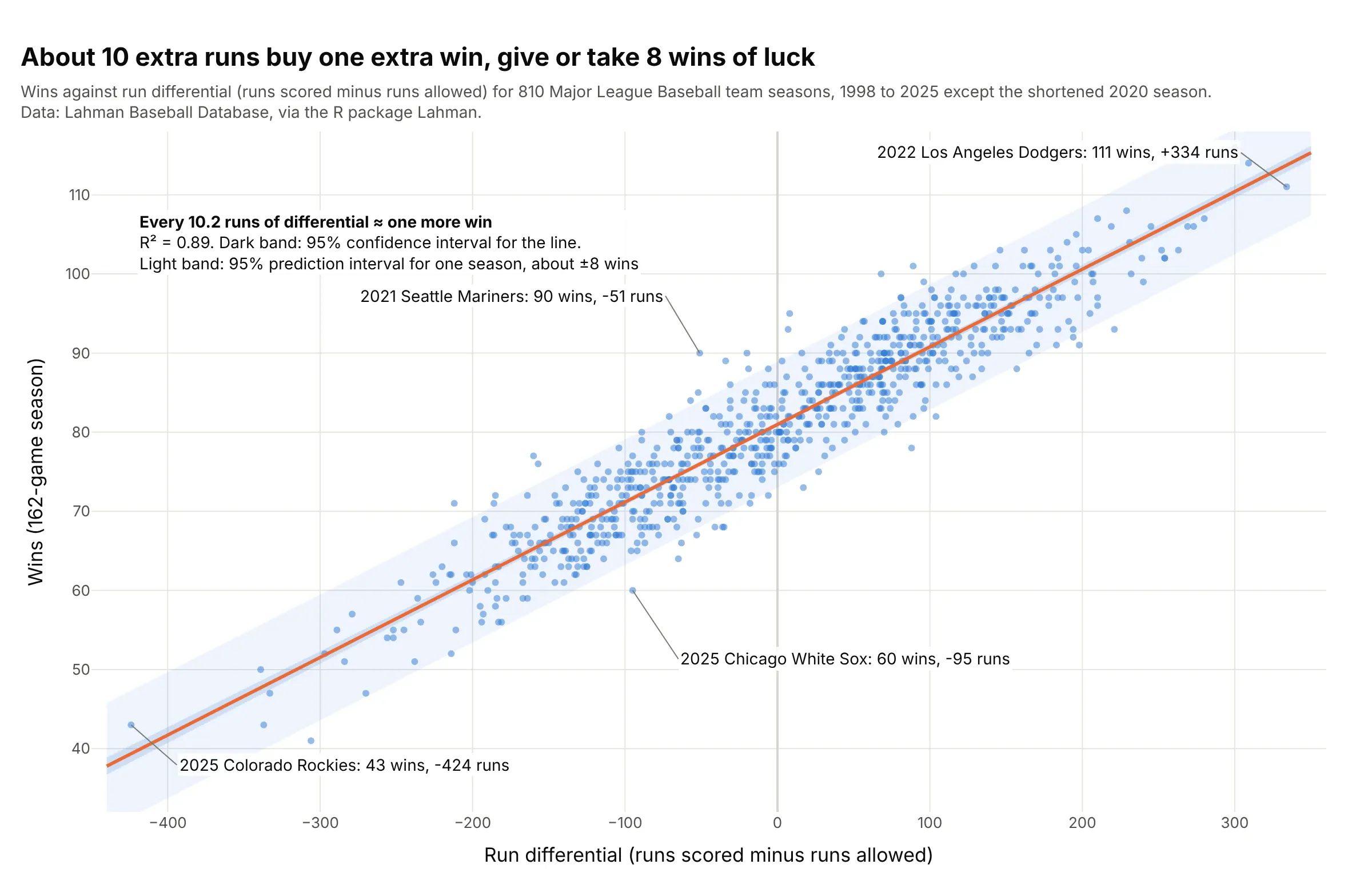
Across 810 team seasons, every 10.2 runs of run differential (runs scored minus runs allowed) was worth one more win, with R² 0.89. The 95% prediction band is about ±8 wins wide: the 2021 Seattle Mariners won 90 games while being outscored by 51 runs, 14 more than the line predicts. Data: Lahman Baseball Database, via the R package Lahman, 1998 to 2025 without the shortened 2020 season.

Tip: shade the prediction band lighter than the confidence band, so readers can see both how well the slope is known and how far a single season strays.