
Chris Parmer
November 15, 2026
Fan Charts - A Complete Guide
TL;DR
- A fan chart draws a forecast as a central line with nested shaded bands around it, each band holding a share of the probability (for example 30%, 60% and 90%), so the bands widen with the horizon and show how uncertain the future is as well as where it is most likely to go.
- A fan chart is a line chart with prediction-interval bands, so it is similar to line charts with a shaded range, error bars at a few dates and regression plots with a prediction band. The Bank of England began publishing its inflation forecast this way in February 1996, and the Federal Reserve and other central banks now draw their projections as fans too.
- Read a fan in slices: the bands at one date are a bell-shaped curve of the possible outcomes, centered on the central projection, and the middle 90% of that curve is the outer band. A band is a probability, so one outcome in ten should still fall outside the widest band.
- You can make a fan chart with Plotly in Python from a few go.Scatter traces with fill="toself", one for each band, and the bands come from a standard deviation, a fitted model's prediction intervals or the central bank's published parameters. A short helper function is below.
What is a fan chart?
Fan charts look like this:
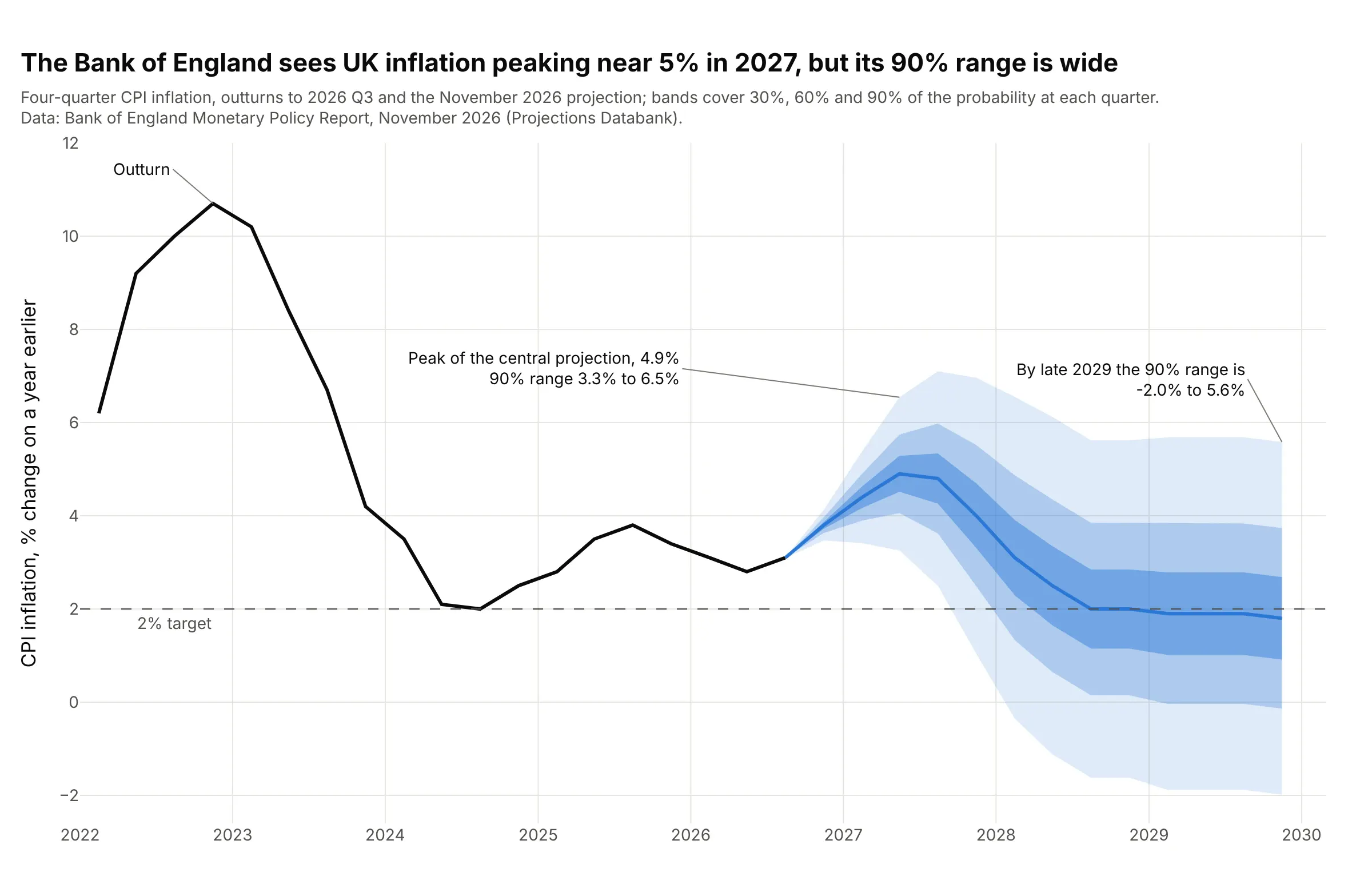
Data: Bank of England Monetary Policy Report, November 2026, Projections Databank (the central projection and the "uncertainty" parameter for each quarter; outturns of four-quarter consumer price index (CPI) inflation, the change in prices over a year).
How do you read a fan chart? In the example above, notice these things:
- The black line is what happened: UK inflation was 3.1% in 2026 Q3. The blue line is the Bank's central projection, the single most likely path (its mode). It rises to 4.9% in 2027 Q2 and returns to 2.0% by 2028 Q3.
- Each shade holds a share of the probability at that quarter. The darkest band holds 30%, the next 60% and the palest 90%, so in 2027 Q2 the 90% band runs from 3.3% to 6.5%.
- The bands widen with the horizon because the future is harder to predict the further away it is. The Bank's uncertainty parameter (a standard deviation) grows from 0.2 percentage points in 2026 Q4 to 2.3 in 2029 Q4, where the 90% band spans 7.6 points, from -2.0% to 5.6%.
- A band is also a probability you can read off. The Bank's own table gives a 97% chance that inflation is above 3% in 2027 Q2, and 30% by the end of 2029, which is the share of the fan above the 3% line at those dates.
It's often used for charts like these:
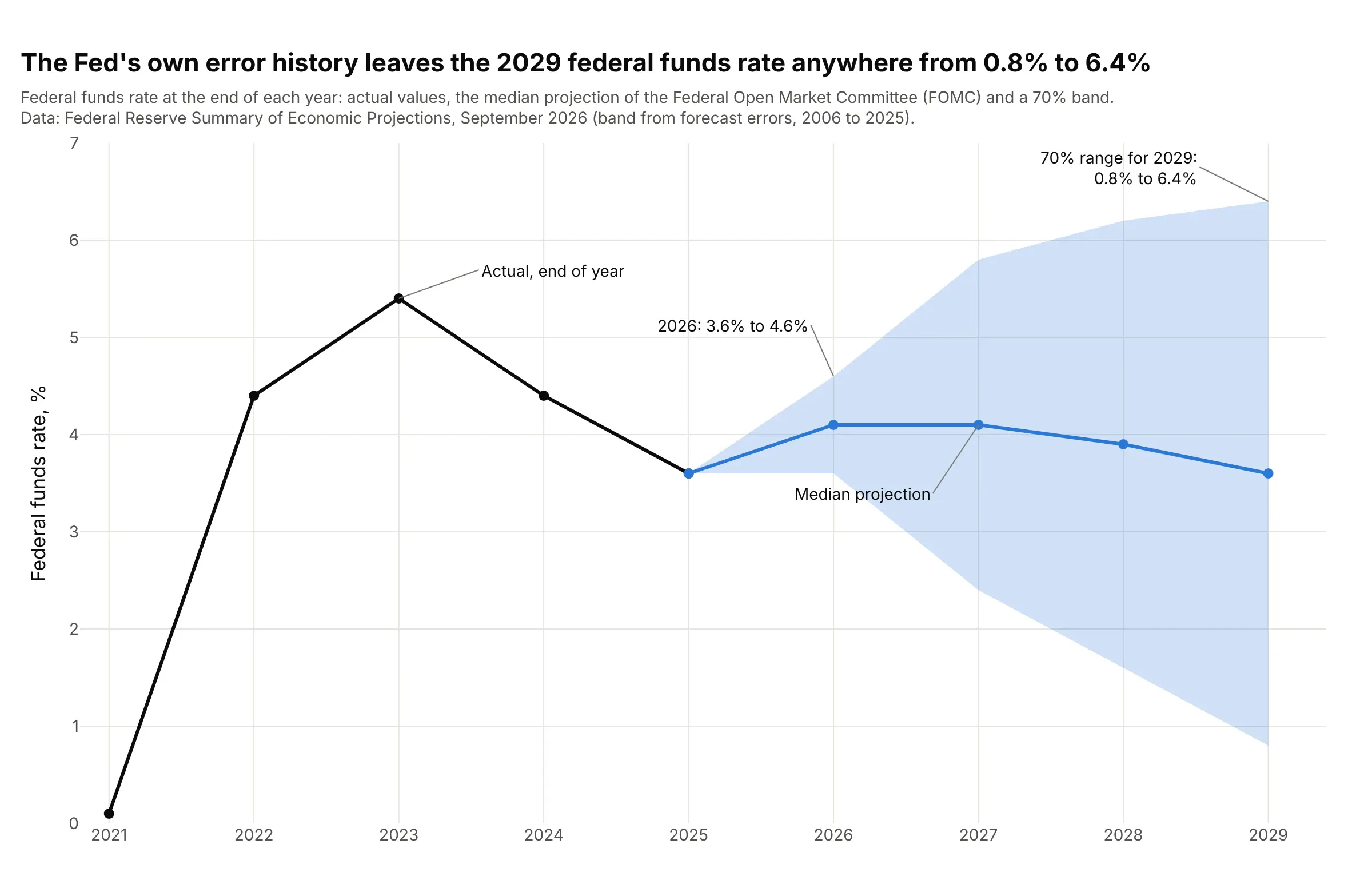
Central bank rate paths. The Federal Reserve draws its federal funds rate projection with a 70% band taken from the size of its own past forecast errors, so the median for 2029 is 3.6% but the band runs from 0.8% to 6.4%, against 3.6% to 4.6% for 2026. Data: Federal Reserve Summary of Economic Projections, September 16, 2026, Figure 5 and Table 2.
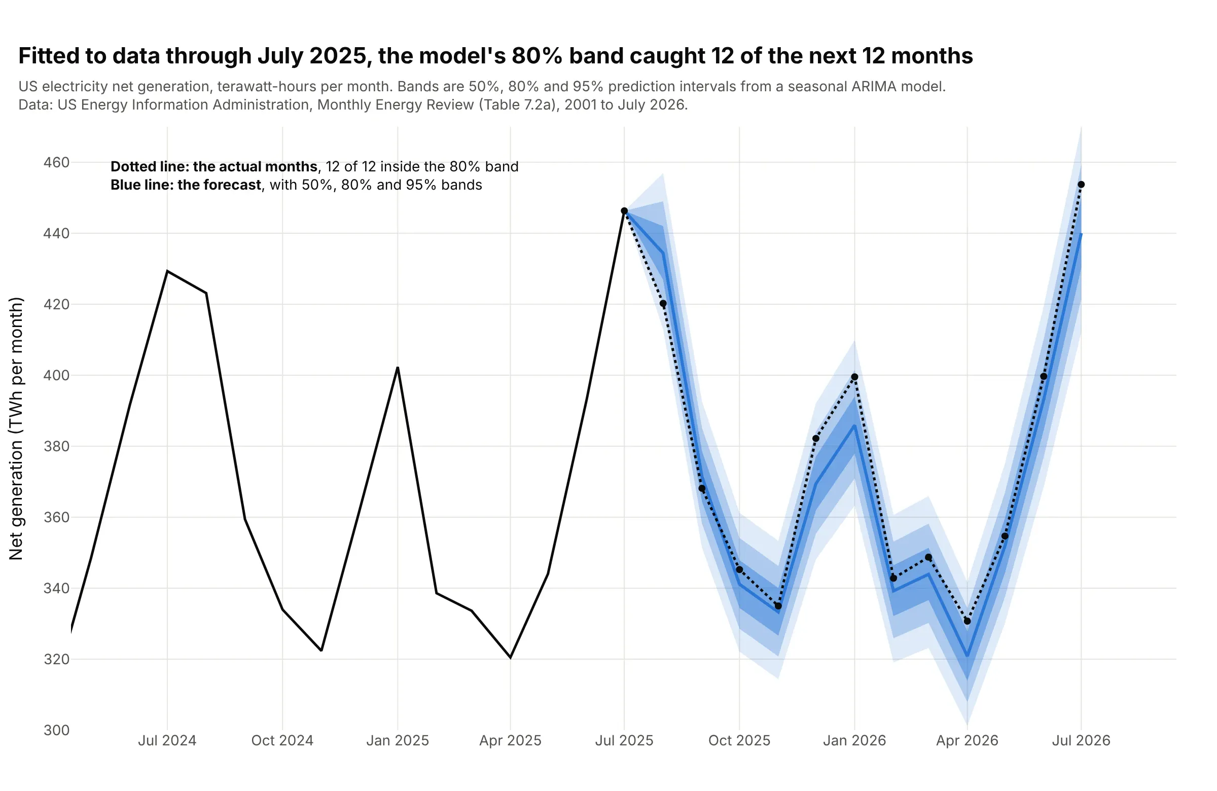
Statistical forecasts you fit yourself. A seasonal model fitted to US electricity generation through July 2025 forecast the next 12 months, and all 12 actual months landed inside its 80% band. Over 16 such forecasts since 2010 (192 months in all), the 50%, 80% and 95% bands held 52%, 83% and 96% of the months. Data: US Energy Information Administration (EIA), Monthly Energy Review, Table 7.2a.
How the bands are calculated
A fan chart looks like shading, but each band is a precise statement about a probability. Knowing where the width comes from makes it easier to trust a fan, or to doubt one, and it is the part a chart library cannot work out for you.
A slice of the fan is a probability distribution
Cut a fan vertically at one date and the bands become a bell-shaped curve. The curve says how likely each outcome is at that date, the peak is the central projection (the mode), and the width of the curve is a standard deviation, which statisticians write as sigma (σ). The Bank of England calls its σ the "uncertainty" parameter:
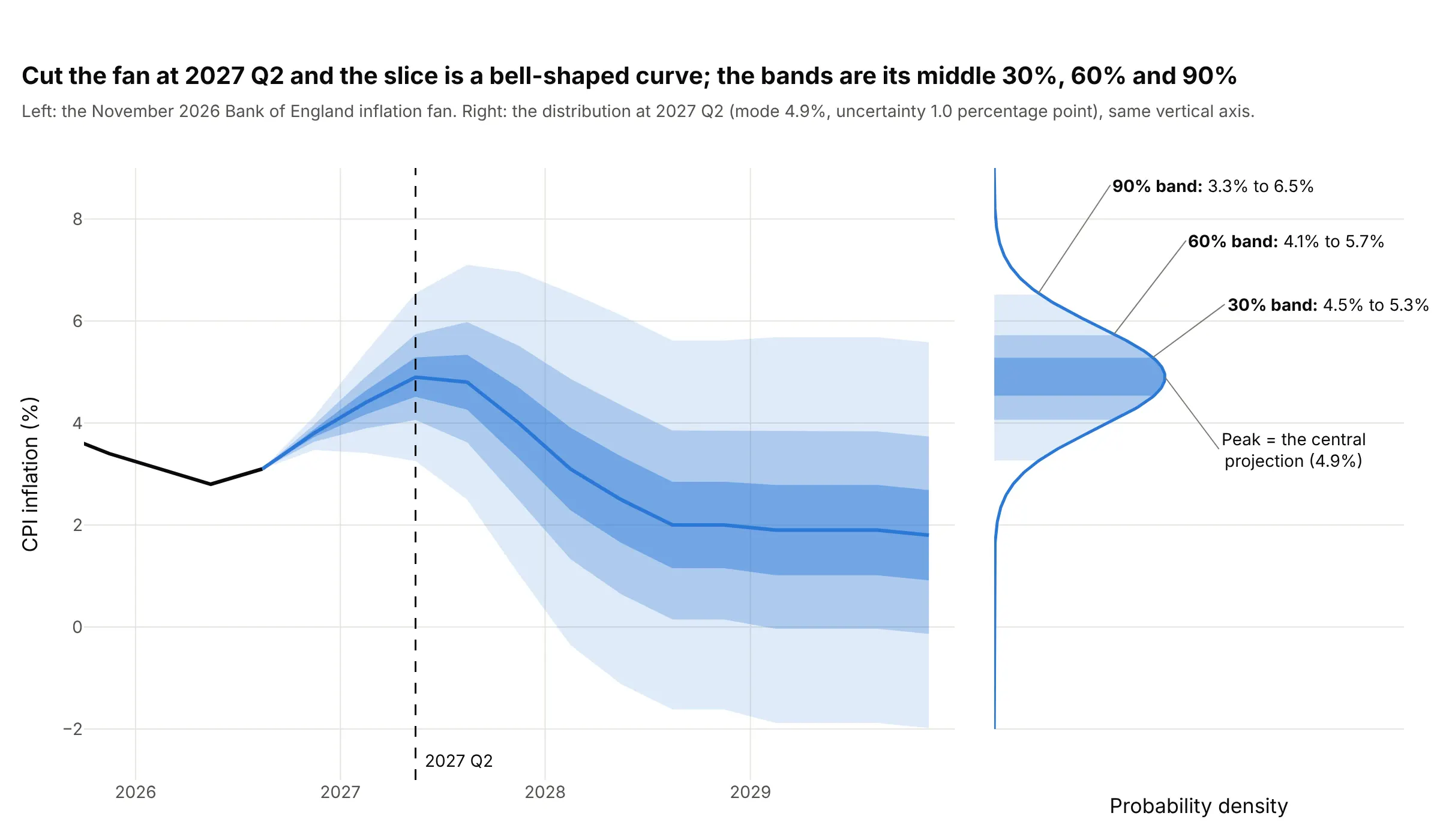
Data: Bank of England Monetary Policy Report, November 2026 (mode 4.9% and uncertainty 1.0 for 2027 Q2).
For a normal (bell-shaped) curve, the middle 30% of the probability lies within 0.385 σ of the center, the middle 60% within 0.84 σ and the middle 90% within 1.645 σ. At 2027 Q2 the mode is 4.9 and σ is 1.0, so the bands are 4.9 ± 0.385 (4.5% to 5.3%), 4.9 ± 0.84 (4.1% to 5.7%) and 4.9 ± 1.645 (3.3% to 6.5%). Those multipliers come from scipy.stats.norm.ppf(0.5 + level / 2), and the check is the Bank's published table: a normal curve with mode 4.9 and σ 1.0 puts 97.1% of the probability above 3%, and the table says 97%.
Where the width comes from
The central line is a forecast. The width is a separate claim about how wrong the forecast tends to be, and the fans in this guide get it in four different ways:
- From past forecast errors. The Federal Reserve takes the root mean squared error (RMSE) of private and government forecasts made in the fall of 2006 through 2025, which grows from 0.5 percentage points for the current year to 2.8 for the fourth year for short-term interest rates (Reifschneider and Tulip, 2017). A band of plus or minus one RMSE holds about 70% of a normal distribution.
- From a fitted model. A time series model such as ARIMA (autoregressive integrated moving average) or exponential smoothing estimates how much random variation is left after fitting, and compounds it step by step, so its prediction intervals widen on their own (examples 3, 4, 6 and 7 below).
- From the market. The Cboe Volatility Index (VIX) is a volatility implied by index option prices, and it converts directly into a width for the next month (example 5).
- From judgment. The Bank of England's Monetary Policy Committee starts from past errors and adjusts the uncertainty and the skew for what it thinks is different this time, which is why its widths change from Report to Report.
Skew and the two-piece normal
If the risks lean one way, the bands should too. The Bank of England draws a bell curve that is wider on one side of its peak, a two-piece normal (or split normal) distribution, which joins two halves of normal curves with the same peak and different spreads (John, 1982). It publishes three numbers for each quarter, the mode, the uncertainty and the skew, defined as the mean minus the mode in percentage points:
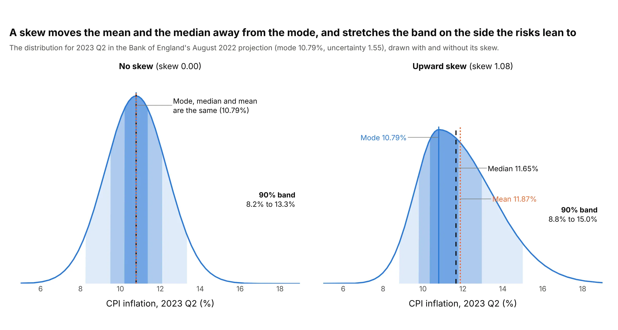
Data: Bank of England parameters for the August 2022 Monetary Policy Report (mode 10.79, uncertainty 1.55, skew 1.08 for 2023 Q2).
With no skew, the mode, median and mean are the same number. With an upward skew, the long tail is on the high side, so the mean sits above the median and both sit above the mode, and the 90% band stretches 4.2 points above the mode but only 2.0 below it. The Bank also draws its bands as the shortest interval holding each share of the probability, so both ends of a band sit at the same height on the curve, which keeps the bands tight around the mode when the curve is lopsided.
What the bands do not say
- Each date has its own bands. A 90% band at one quarter does not mean the whole path stays inside the fan with 90% probability, because a path can leave the fan at one date and come back.
- A band is a probability, not a bound. One outcome in ten should fall outside a 90% band, and example 2 below counts how often that happened.
- A prediction interval is wider than a confidence interval. A confidence interval says how well the average is known, and a prediction interval also holds the scatter of a single future value. A fan shows the second one, as example 7 shows for a trend line. The regression plot and error bars guides explain the difference for fitted lines.
- The width depends on assumptions. A fan from past errors assumes the future is about as hard to predict as the past, and a Bank of England projection is conditional on the interest rates, exchange rates and energy prices it assumes.
A short history
Before 1996, the Bank of England's inflation forecast was a line with a shaded area drawn from the average size of past forecast errors, which readers often took for upper and lower bounds. From February 1996 the Bank published its forecast as a probability distribution drawn as a fan, and in 1998 Erik Britton, Paul Fisher and John Whitley described how it is made: a central projection as the mode, an uncertainty taken from past errors and a skew for the balance of risks, drawn in 10% bands out to 90%. Wikipedia credits the Bank with the name fan chart. Sweden's Riksbank described its own uncertainty bands for inflation forecasts in a 1998 working paper (Blix and Sellin), the Federal Reserve draws a fan built from historical errors in its Summary of Economic Projections, and Guy Abel's fanplot package brought the chart to the R language. We couldn't find the data behind the 1996 chart in a public form to redraw it, so example 1 below draws the same kind of chart for the Bank's August 2022 projection from its published parameters.
Alternatives to a fan chart
Here's the same Bank of England projection drawn six ways. Some are better for the question, some worse, some just different:
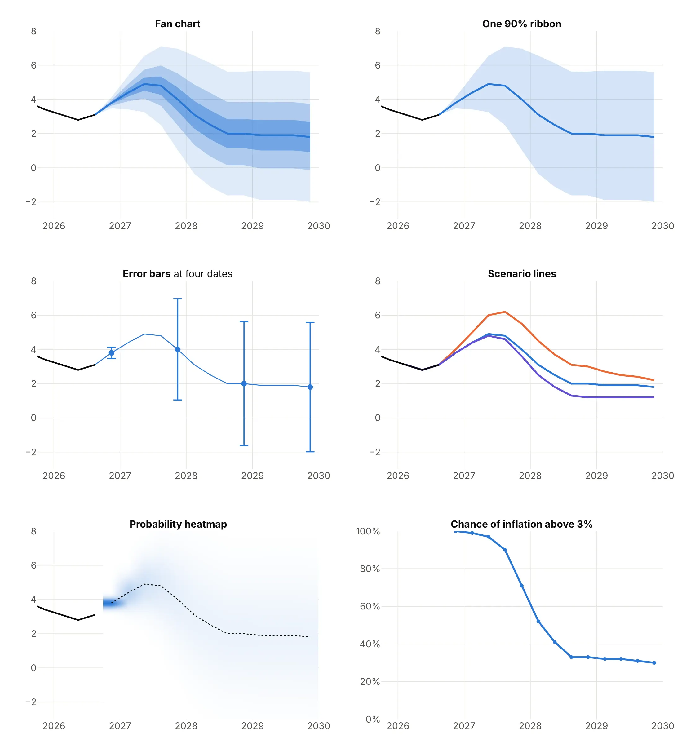
- Fan chart (best for a forecast with its uncertainty). It shows the central path, the spread and how the spread grows, for every date at once.
- One 90% ribbon (works too, for one question). A line chart with a shaded range is simpler and fine when only the outer limit matters, but it hides where the likely outcomes are and makes the edge look like a bound.
- Error bars (works too, at a few dates). They give exact ranges at chosen dates, such as 3.5% to 4.1% in 2026 Q4 and -2.0% to 5.6% in 2029 Q4, but lose the continuous widening.
- Scenario lines (different). The Bank's weaker demand and adverse inflation scenarios peak at 4.8% and 6.0% in 2027 Q2 against 4.9% in the central projection. Scenarios answer "what if?" with a few named stories and say nothing about how likely each one is.
- Heatmap of probability (works too, harder to read). Color shows the probability at every value and quarter, which is the most complete picture, but readers cannot read a band's edges off a color scale.
- Probability of crossing a threshold (different). The Bank's table gives a 97% chance of inflation above 3% in 2027 Q2, falling below 50% by 2028 Q2. It answers one question precisely, and the fan answers that question and every other one.
How to make a fan chart
With AI
ChatGPT, Claude Code, GitHub Copilot, Cursor and other AI tools are excellent at writing Plotly code. Name Plotly in the prompt, and say where the bands come from and how wide each one should be:
Make a plotly fan chart from cpi_projection.csv (columns: quarter, kind, value, uncertainty; kind is "outturn" or "projection").- Draw the outturns as a black line, then the projection as a blue line with three bands around it:value +/- z x uncertainty, with z = scipy.stats.norm.ppf(0.5 + level / 2) for levels 0.9, 0.6 and 0.3.- Draw each band as one go.Scatter polygon with fill="toself", widest first, in the same blue at opacity 0.15, 0.28 and 0.45.- Start the bands at the last outturn with zero width so the fan grows out of the history.- Add a dashed line at 2 (the target), a title that states the takeaway, and an axis title "CPI inflation (%)".- Check: print the 90% band for the quarter with the highest value.
With Plotly Studio
Plotly Studio is a product for creating data visualizations and Dash apps and for analyzing data with AI, available as a desktop app or embedded in Dash apps. Ask for a fan chart the same way:
Show a fan chart of the next 12 months of US electricity generation from a seasonal model, with 50%, 80% and 95% prediction bands in one blue, the actual months as a dotted line, and a dropdown to switch between the 12-month and 24-month horizon.
In Python or JavaScript
This is the code AI tools write under the hood. In Python, a fan chart is a set of filled polygons, one per band, with a line on top. The helper below takes a central path and a standard deviation at each step, and draws the widest band first so the narrower ones sit on top:
import numpy as npimport pandas as pdimport plotly.graph_objects as gofrom scipy import statsdef add_band(fig, x, low, high, alpha, name=None):"""One shaded band between two paths, drawn as a closed polygon."""fig.add_trace(go.Scatter(x=list(x) + list(x)[::-1], y=list(high) + list(low)[::-1], fill="toself",fillcolor=f"rgba(42,120,214,{alpha})", line=dict(width=0), hoverinfo="skip", name=name))def fan_chart(x, center, sigma, levels=(0.9, 0.6, 0.3)):"""Nested bands around a central path. sigma is the standard deviation at each x."""center, sigma = np.asarray(center), np.asarray(sigma)fig = go.Figure()for lv, alpha in zip(levels, (0.15, 0.28, 0.45)): # widest band first, so the narrow ones sit on topz = stats.norm.ppf(0.5 + lv / 2) # 1.645 for 90%, 0.84 for 60%, 0.385 for 30%add_band(fig, x, center - z * sigma, center + z * sigma, alpha, f"{lv:.0%} band")fig.add_trace(go.Scatter(x=x, y=center, mode="lines", line=dict(color="#2a78d6", width=3), name="Central projection"))return figdf = pd.read_csv("cpi_projection.csv") # columns: quarter, kind ("outturn" or "projection"), value, uncertaintyhist, proj = df[df.kind == "outturn"].tail(8), df[df.kind == "projection"]fig = fan_chart(proj.quarter, proj.value, proj.uncertainty)fig.add_trace(go.Scatter(x=hist.quarter, y=hist.value, mode="lines", line=dict(color="black", width=3), name="Outturn"))fig.update_xaxes(categoryorder="category ascending")fig.update_layout(yaxis_title="CPI inflation (%)")fig.show()
When the bands come from a fitted model, skip the standard deviation and pass the model's prediction intervals to add_band. With statsmodels, get_forecast(...).conf_int(alpha=...) returns the lower and upper bound of an interval for each step, and the code below draws 50%, 80% and 95% bands for a seasonal model of electricity generation:
import numpy as npimport pandas as pdimport plotly.graph_objects as gofrom statsmodels.tsa.statespace.sarimax import SARIMAXy = pd.read_csv("generation.csv", parse_dates=["month"]).set_index("month").gwh.asfreq("MS") # columns: month, gwhfit = SARIMAX(np.log(y), order=(1, 1, 1), seasonal_order=(0, 1, 1, 12)).fit(disp=False) # a model of the log of generationforecast = fit.get_forecast(12)fig = go.Figure()for level, alpha in ((0.95, 0.15), (0.8, 0.28), (0.5, 0.45)):ci = np.exp(forecast.conf_int(alpha=1 - level)) # prediction interval, back on the original scaleadd_band(fig, ci.index, ci.iloc[:, 0], ci.iloc[:, 1], alpha, f"{level:.0%} band") # add_band is defined abovefig.add_trace(go.Scatter(x=y.index[-36:], y=y[-36:], mode="lines", line=dict(color="black"), name="Actual"))fig.add_trace(go.Scatter(x=forecast.predicted_mean.index, y=np.exp(forecast.predicted_mean), mode="lines",line=dict(color="#2a78d6", width=3), name="Forecast"))fig.show()
Fitting the model to the log of the series keeps the bands positive and makes them lopsided on the original scale, which is what example 6 relies on. For skewed fans like the Bank of England's, compute the band edges from the two-piece normal instead of from norm.ppf; the options at the end link the reference pages.
In JavaScript, plotly.js draws the same thing with one filled scatter trace per band. The bands are mode plus or minus z times the uncertainty, with the z scores for 90%, 60% and 30% written out:
<div id="chart"></div><script src="https://cdn.plot.ly/plotly-4.1.1.min.js"></script><script>// Bank of England, November 2026 Monetary Policy Report: four-quarter CPI inflation (%)const past = {q: ["2024Q4", "2025Q1", "2025Q2", "2025Q3", "2025Q4", "2026Q1", "2026Q2", "2026Q3"],y: [2.5, 2.8, 3.5, 3.8, 3.4, 3.1, 2.8, 3.1]};const quarters = ["2026Q4", "2027Q1", "2027Q2", "2027Q3", "2027Q4", "2028Q1", "2028Q2", "2028Q3", "2028Q4", "2029Q1", "2029Q2", "2029Q3", "2029Q4"];const mode = [3.8, 4.4, 4.9, 4.8, 4.0, 3.1, 2.5, 2.0, 2.0, 1.9, 1.9, 1.9, 1.8]; // central projectionconst sigma = [0.2, 0.6, 1.0, 1.4, 1.8, 2.1, 2.2, 2.2, 2.2, 2.3, 2.3, 2.3, 2.3]; // "uncertainty": the standard deviation// z scores for the middle 90%, 60% and 30% of a normal distributionconst bands = [{z: 1.645, alpha: 0.15, name: "90% band"}, {z: 0.842, alpha: 0.28, name: "60% band"}, {z: 0.385, alpha: 0.45, name: "30% band"}];const x = [past.q[past.q.length - 1], ...quarters]; // start the fan at the last outturn, with zero widthconst m = [past.y[past.y.length - 1], ...mode], s = [0, ...sigma];const fan = bands.map(b => ({type: "scatter", mode: "lines", name: b.name, hoverinfo: "skip",x: [...x, ...[...x].reverse()],y: [...m.map((v, i) => v + b.z * s[i]), ...m.map((v, i) => v - b.z * s[i]).reverse()],fill: "toself", fillcolor: `rgba(42,120,214,${b.alpha})`, line: {width: 0}}));Plotly.newPlot("chart", [{type: "scatter", mode: "lines", x: past.q, y: past.y, name: "Outturn", line: {color: "black", width: 3}},...fan,{type: "scatter", mode: "lines", x: x, y: m, name: "Central projection", line: {color: "#2a78d6", width: 3}}], {width: 900, height: 520, yaxis: {title: {text: "CPI inflation (%)"}}, xaxis: {type: "category"},title: {text: "Bank of England CPI inflation projection, November 2026"}});</script>
Share it
Every Plotly chart has a Share chart button (the cloud icon in its toolbar) that uploads it to Plotly Cloud and gives you a link. Only you can see it until you change its visibility.
For a live app, put the chart in a Dash app and publish it with the Plotly Cloud command-line interface (CLI). Coding agents can run these commands for you:
pip install "dash[cloud]"plotly user loginplotly app publish
If your data has to stay in your own cloud or data center, publish to Dash Enterprise instead.
Dos and don'ts
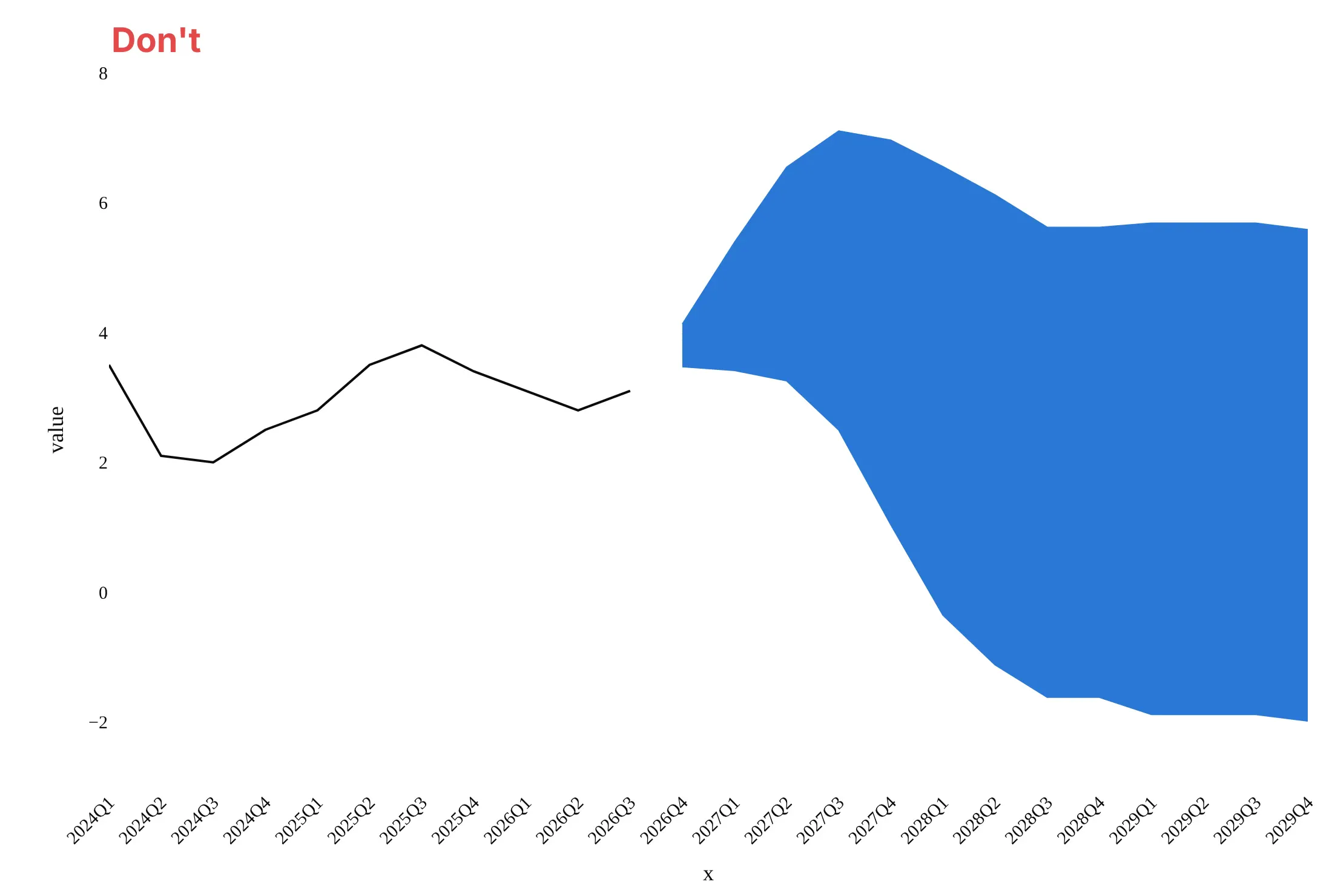
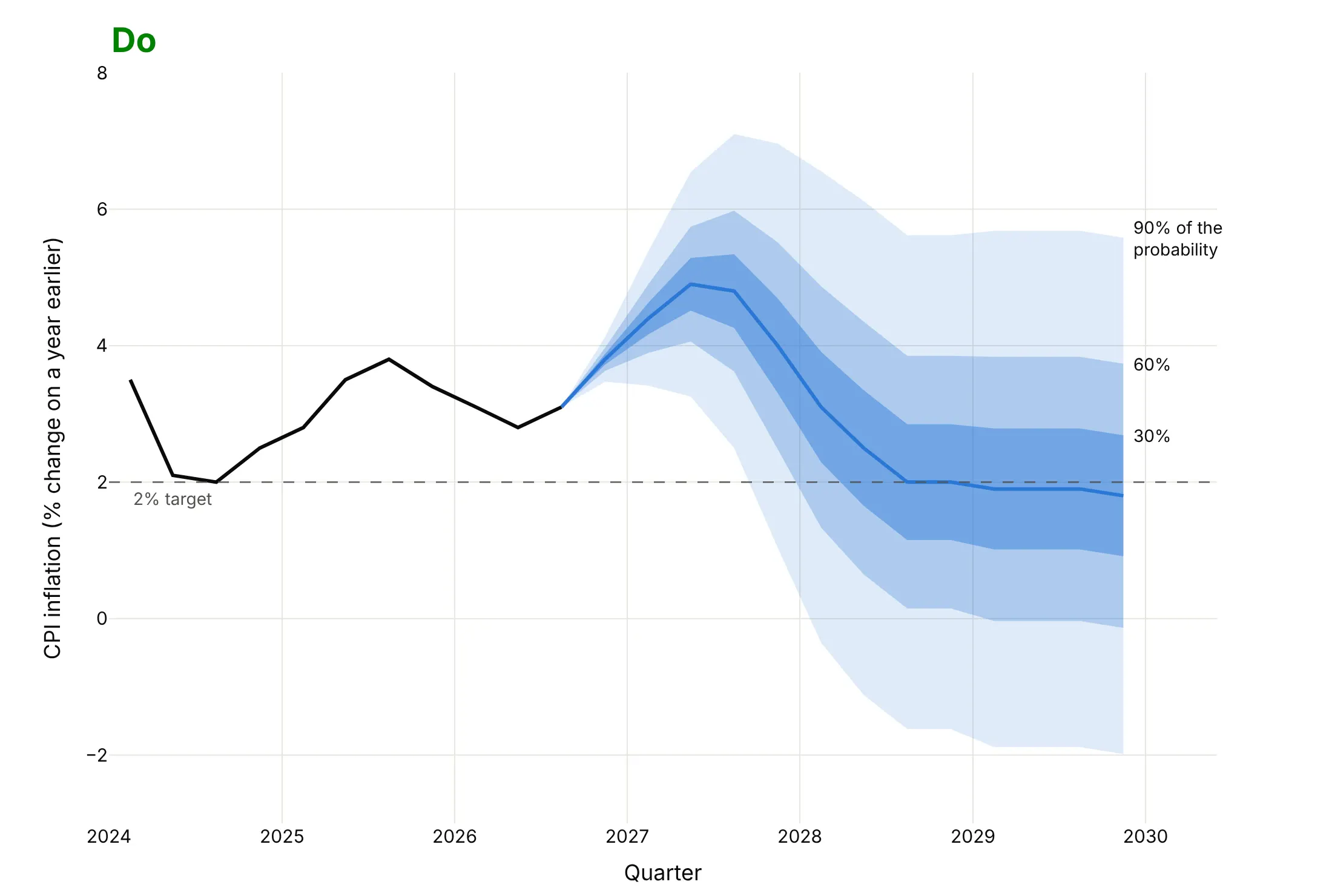
A fan chart is easy to get technically right and hard to read, because the shading carries the meaning. Here is the Bank of England projection both ways, in the same blue.
Don't draw the bands in one opaque color so the nesting disappears, leave a gap between the history and the fan, leave out the central line and the target, use column names as axis titles, or keep a default serif font:
Do draw translucent bands that get lighter outward, start the fan at the last observation, draw the central projection, mark the target, label what each band holds and write axis titles in words with units:
Checklist
Do
- Say what the bands hold ("30%, 60% and 90% of the probability") and where the width comes from (past errors, a model, the market or judgment).
- Use one hue, lighter toward the outside, and no more than four bands.
- Start the fan at the last observation with zero width, so it grows out of the history.
- Draw the central line, and mark a target, threshold or zero line the reader will compare with.
- Model positive data such as prices on a log scale, so the fan stays above zero and shows the long upper tail.
- Check the fan against outcomes (examples 2, 4, 5 and 6) before you trust its width.
Don't
- Draw only the upper and lower lines of the widest band, which reads as best and worst case.
- Call a 90% band a range outcomes will stay in, or read the fan as a set of possible paths.
- Use a symmetric band when the risks are not symmetric, such as a rate that cannot fall below zero.
- Hide the assumptions the projection is conditioned on, such as interest rates or energy prices.
More fan chart examples
Seven more fan charts built from real public data, each with its source, the technique that makes it work and a prompt to rebuild it.
1. A skewed fan: the Bank of England's August 2022 projection
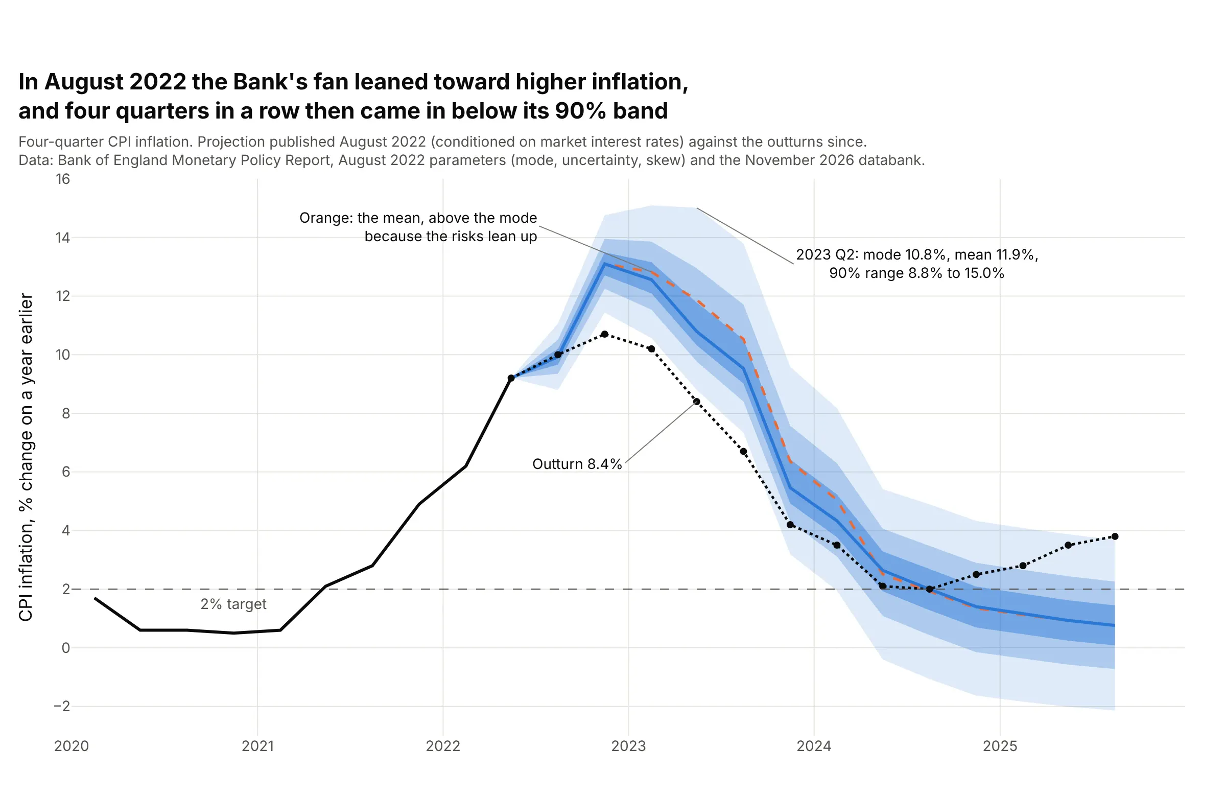
In August 2022 the Bank's fan was wider above its central projection than below it (skew 1.08 in 2023 Q2), which put the mean 1.1 points above the mode. Inflation then came in below the 90% band for four quarters in a row, from 10.7% against a band starting at 11.4% in 2022 Q4 to 6.7% against 7.3% in 2023 Q3. Data: Bank of England parameters for the August 2022 projection (published in the August 2025 download) and outturns from the November 2026 Projections Databank.
Tip: draw the mean as a second dashed line next to the mode, so a skew shows up as a gap between them.
Get the data from the Bank of England: the "Parameters for MPC CPI inflation projections from February 2004" workbook in theAugust 2025 Monetary Policy Report download (sheet CPI Forecast, the projection conditioned on market interest rates: mode, median,mean, uncertainty and skew for each quarter of each Report) and the outturns of four-quarter CPI inflation from the November 2026Projections Databank (columns: report, quarter, mode, mean, uncertainty, skew, outturn).Build a plotly fan chart for the August 2022 Report: split the uncertainty and skew into the two standard deviations of a two-piecenormal, draw the 30%, 60% and 90% bands as the shortest intervals (equal density at both ends), the mode as a blue line, the meanas a dashed orange line and the outturns as a dotted black line, and label the first quarter where the outturn leaves the 90% band.
2. How often did inflation land inside the Bank of England's bands?
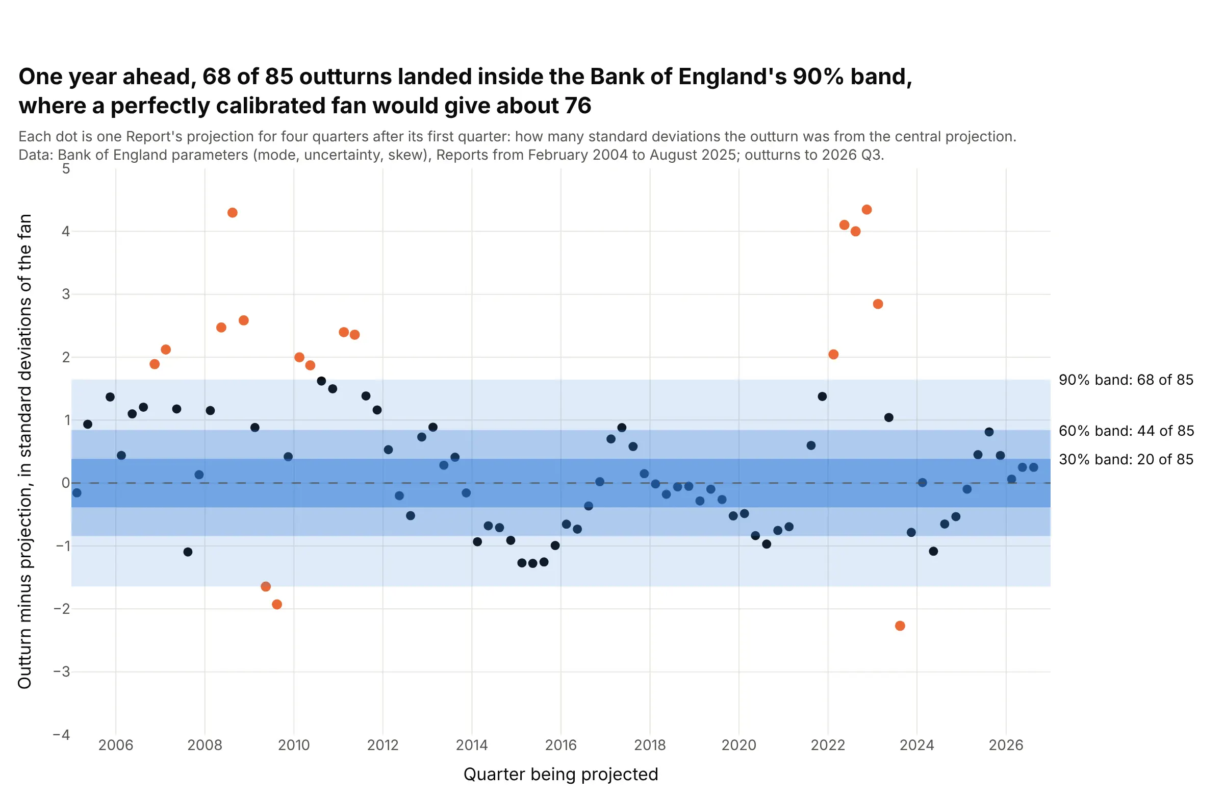
Of 85 Reports from February 2004 to August 2025, the inflation outturn four quarters after the first projected quarter landed inside the 90% band 68 times, where a perfectly calibrated fan would give about 76, and inside the 30% band 20 times, where it would give about 25. Of the 17 misses, 14 were above the fan, clustered from 2007 to 2011 and in 2022. Data: Bank of England projection parameters and outturns, as in example 1.
Tip: divide each miss by the fan's own width (a z score), so every Report shares one set of bands and the pattern over time is visible.
Get the data from the Bank of England: the "Parameters for MPC CPI inflation projections from February 2004" workbook in theAugust 2025 Monetary Policy Report download (mode, uncertainty and skew by quarter for each Report, market-conditioned) and theoutturns of four-quarter CPI inflation from the November 2026 Projections Databank (columns: report, quarter, mode, uncertainty, skew, outturn).For the quarter four after each Report's first, compute the outturn's position in the two-piece normal distribution (its probabilityintegral transform), turn it into a z score with scipy.stats.norm.ppf, and build a plotly scatter of z against the quarter withhorizontal bands at +/-0.385, 0.84 and 1.645 for 30%, 60% and 90%, points outside the 90% band in orange, and the count inside each band annotated.
3. A fan that crosses zero: the Bank of England's GDP projection
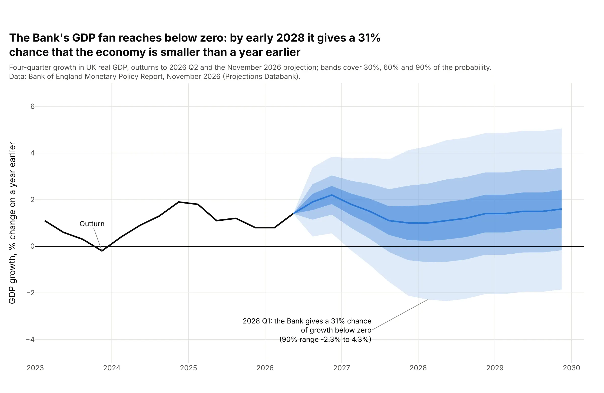
The Bank's central projection for four-quarter gross domestic product (GDP) growth never falls below 1.0%, but its uncertainty reaches 2.0 points by 2028 Q1, so the 90% band spans -2.3% to 4.3% and the Bank gives a 31% chance that the economy is smaller than a year earlier. Data: Bank of England Monetary Policy Report, November 2026 (Projections Databank, GDP growth and its distribution).
Tip: draw the zero line heavier than the grid and annotate the published probability, so readers can tell the shaded area below zero is a number.
Get the data from the Bank of England November 2026 Monetary Policy Report "Projections Databank" workbook: sheet "2. GDP growth" (last row:outturns then the central projection of four-quarter GDP growth) and sheet "40. GDP growth distribution" (the uncertainty by quarter and thepublished probability of growth below 0%) (columns: quarter, kind, value, uncertainty, prob_below_zero).Build a plotly fan chart from 2023: 30%, 60% and 90% bands as mode +/- z x uncertainty, a heavy line at zero, and an annotation ofthe published probability of growth below zero for 2028 Q1 with the 90% range.
4. Carbon dioxide at Mauna Loa: a fan that holds its width and misses its trend
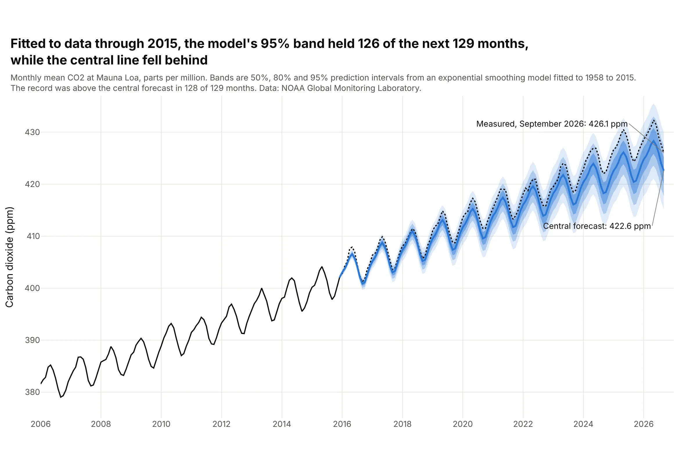
An exponential smoothing model fitted to the Mauna Loa record through 2015 forecast the next 129 months. The 95% band held 126 of them (98%) and the 80% band 119, but the record was above the central line in 128, and only 24 months fell inside the 50% band, because growth sped up after 2015: 426.1 parts per million (ppm) in September 2026 against 422.6 forecast. Data: National Oceanic and Atmospheric Administration (NOAA) Global Monitoring Laboratory, Mauna Loa monthly mean CO2.
Tip: fit on the past only and overlay the measured values, so the reader sees what the bands got right (the spread) and what they missed (the trend).
Get the data from NOAA Global Monitoring Laboratory: the Mauna Loa Observatory monthly mean carbon dioxide record(https://gml.noaa.gov/webdata/ccgg/trends/co2/co2_mm_mlo.csv, "average" column in ppm, since March 1958) (columns: month, ppm).Fit statsmodels ETSModel(error="add", trend="add", seasonal="add", seasonal_periods=12) on data through December 2015, get 50%, 80% and95% prediction intervals to September 2026 with get_prediction().summary_frame(alpha), and build a plotly fan chart with the measuredrecord as a dotted line and the count of months inside the 95% band in the title.
5. The S&P 500 over the next month, from the VIX
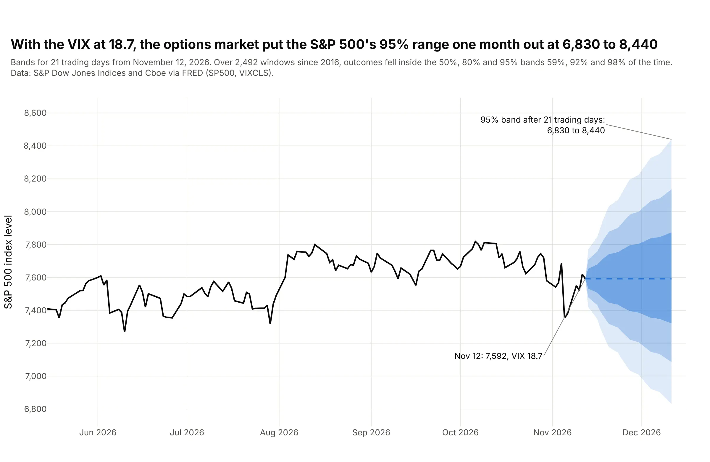
With the VIX at 18.7 on November 12, 2026, a log-normal price distribution puts the S&P 500's 95% range 21 trading days out at 6,830 to 8,440, from 7,592 today. Over 2,492 such windows since 2016 the outcomes fell inside the 50%, 80% and 95% bands 59%, 92% and 98% of the time, so the options market's width was a little too wide. Data: S&P Dow Jones Indices (S&P 500) and Cboe (VIX) via Federal Reserve Economic Data (FRED).
Tip: scale the width with the square root of time (VIX / 100 x sqrt(n / 252)) and exponentiate the bands, so the fan flares from a point and stays positive.
Get the data from Federal Reserve Economic Data (FRED): series SP500 (S&P 500 index, daily, last ten years) and VIXCLS (CboeVolatility Index close) (columns: date, sp500, vix).Build a plotly fan chart for the next 21 trading days from the last date: median at today's level, log-normal bands at 50%, 80% and95% with sigma = vix/100 x sqrt(n/252), six months of history in black, and in the subtitle the share of all past 21-day windowswhose outcome fell inside each band.
6. Natural gas prices: a fan that is skewed because prices stay positive
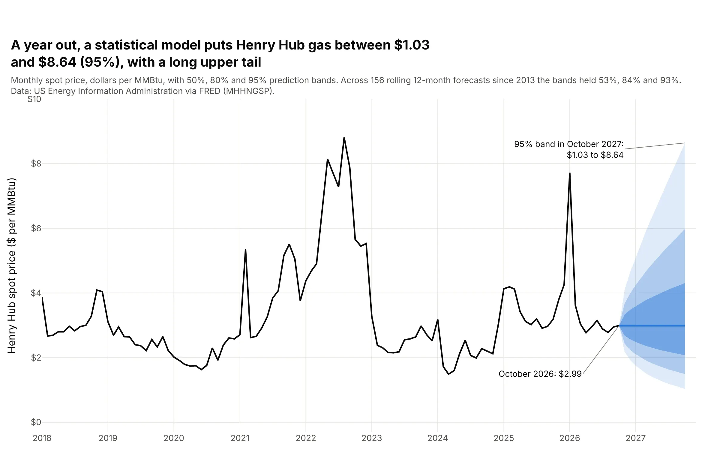
A model of the log of the Henry Hub natural gas price puts the 95% band for October 2027 at $1.03 to $8.64 per million British thermal units (MMBtu), against $2.99 in October 2026, which leaves $1.96 of room below the central line and $5.65 above it. Across 156 rolling 12-month forecasts since 2013, the 50%, 80% and 95% bands held 53%, 84% and 93% of the months. Data: EIA, Henry Hub spot price via FRED.
Tip: fit the model to the log of the price and exponentiate the bands, so the lower edge cannot fall below zero.
Get the data from the US Energy Information Administration: the monthly Henry Hub natural gas spot price, dollars per MMBtu(FRED series MHHNGSP) (columns: month, price).Fit statsmodels ARIMA(1,1,0) to the log of the price from 2000, get 50%, 80% and 95% prediction intervals for the next 12 months,exponentiate them and build a plotly fan chart with the history from 2018, and check the intervals by rolling origin: fit on data toeach October from 2013 to 2025 and count the share of the next 12 months inside each interval.
7. A trend and its two kinds of uncertainty: global temperature
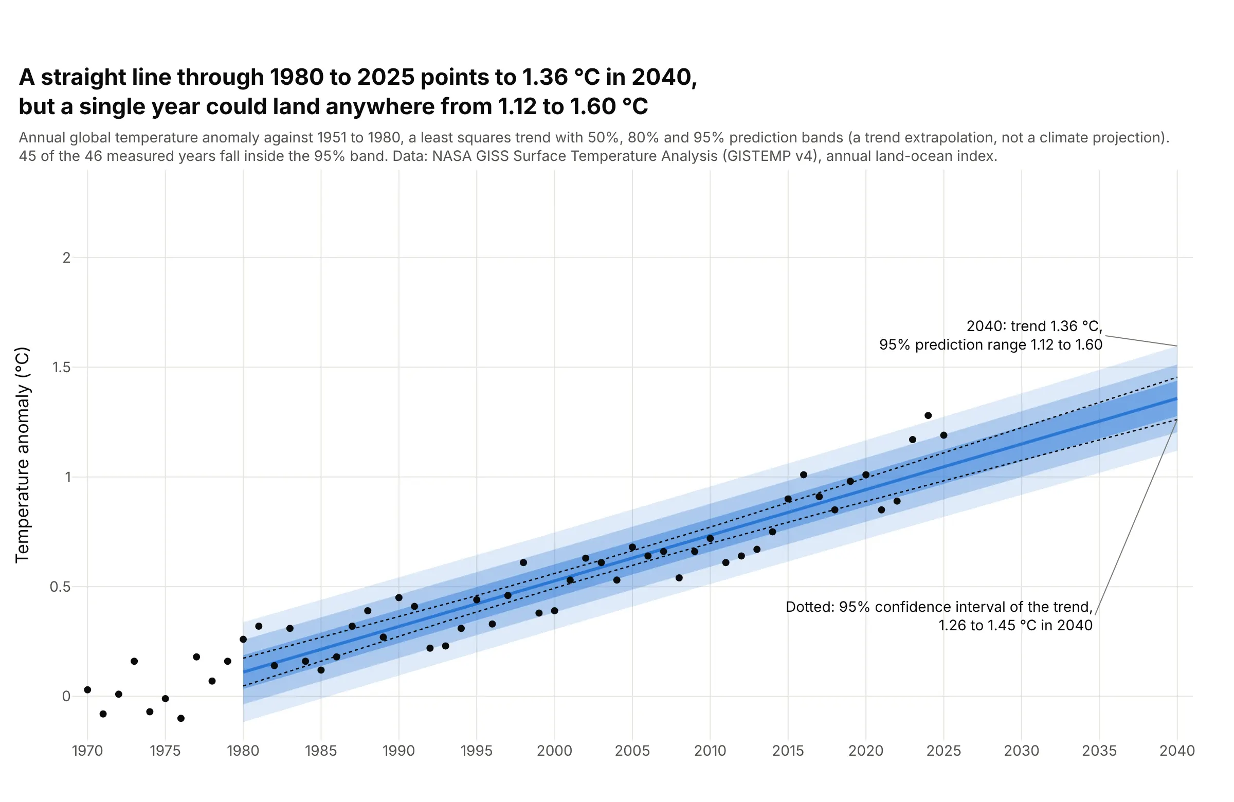
A straight line through the 1980 to 2025 anomalies warms by 0.21 °C per decade and reaches 1.36 °C in 2040. The 95% confidence interval of that line is 1.26 °C to 1.45 °C, but a single year's 95% prediction range is 1.12 °C to 1.60 °C, and 45 of the 46 measured years fall inside it. This is a trend extrapolation and not a climate projection. Data: NASA Goddard Institute for Space Studies, GISTEMP v4 annual global land-ocean temperature index.
Tip: draw the confidence interval of the trend as thin dotted lines inside the fan, so the gap between the two kinds of interval is the lesson.
Get the data from NASA Goddard Institute for Space Studies, GISTEMP v4 global-mean annual (J-D) land-ocean temperature index in degreesCelsius against 1951 to 1980 (https://data.giss.nasa.gov/gistemp/tabledata_v4/GLB.Ts+dSST.csv) (columns: year, anomaly).Fit statsmodels OLS of anomaly on year for 1980 to 2025, call get_prediction on the years 1980 to 2040, and build a plotly chart with50%, 80% and 95% prediction bands (obs_ci_lower and obs_ci_upper) as a fan, the 95% confidence interval of the mean as dotted lines,the yearly values as dots from 1970 and the 2040 values annotated.
FAQ
Options to customize
A fan chart in Plotly is a few filled scatter traces plus a line, so these are the options that matter most. The full lists are in the scatter trace reference, the scattergl trace reference, the filled area guide and the shapes guide.
- fill="toself" with the x values forward and then backward: one closed polygon per band, which handles bands of any shape and any order of drawing.
- fill="tonexty": the alternative, with an upper line and then a lower line for each band, so the lower trace fills up to the one before it. It needs the traces in a strict order.
- fillcolor="rgba(42,120,214,0.15)": the band color with its opacity, lighter for the wider bands so the nesting reads as depth.
- line.width=0 and hoverinfo="skip": no outline on a band and no hover box on its edges, so the central line carries the hover.
- scipy.stats.norm.ppf(0.5 + level / 2): the z multiplier for a central band of a normal distribution; for skewed fans use the two-piece normal's own quantiles.
- get_forecast(...).conf_int(alpha=...): a fitted model's prediction interval at each step, in statsmodels, and ETSModel(...).fit().get_prediction().summary_frame(alpha) for exponential smoothing.
- np.exp(...) on bands fitted to a log series: bands that stay positive and lean toward the upper tail, as in the natural gas example.
- fig.add_hline(y=2), fig.add_vline(x=...) and fig.add_vrect(...): a target line, a boundary between history and forecast and a shaded forecast period.
- error_y(type="data", symmetric=False, array=..., arrayminus=...): error bars at chosen dates, for the alternative that gives exact ranges.
- go.Scattergl: WebGL traces for line series with many points, with the caveat that filled bands of 100,000 steps failed in our test, so draw those bands with the SVG trace.
- fig.add_annotation(...) with ax and ay: labels with leader lines for the peak, the band edges at a date and the probability of crossing a threshold.
- customdata and hovertemplate on the central line: the band edges in the hover text, so one hover gives the value and its 90% range.
- xaxis.categoryorder="category ascending": keeps quarter codes such as 2026Q4 in order when the history and the projection are separate traces.