
Chris Parmer
November 18, 2026
3D Scatter Plots - A Complete Guide
TL;DR
- A 3D scatter plot places each observation as a point at three coordinates (x, y and z), so you can rotate the cloud and see structure that two axes hide. It works best when all three axes are real dimensions, such as longitude, latitude and depth, or when the question is about the shape of a point cloud.
- 3D scatter plots are also known as 3D scatterplots and 3D point clouds, and the same chart drawn with lines between the points is a 3D line chart or 3D line plot (MATLAB calls them scatter3 and plot3). They are similar to scatter plots, scatter plot matrices, bubble charts and 3D surface plots.
- They are easy to misread: points in front hide points behind them, and a still image from the wrong angle can make clusters look merged or separate. For precise comparisons, a scatter plot with color for the third variable, a scatter plot matrix or small multiples are easier to read, and a good 3D scatter plot is one you can rotate.
- You can make a 3D scatter plot with Plotly from px.scatter_3d or go.Scatter3d (and a 3D line chart with mode="lines"), in Python or JavaScript. In our test, 100,000 points drew in about 1 second and 500,000 in about 5 seconds.
What is a 3D scatter plot?
3D scatter plots look like this:
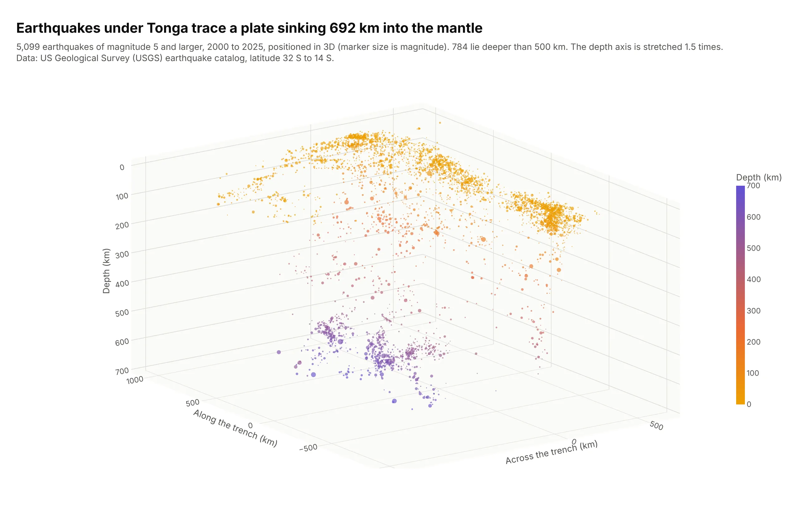
Data: US Geological Survey (USGS) earthquake catalog, magnitude 5 and larger, latitude 32 S to 14 S, 2000 to 2025. Positions are kilometers from 23 S, 177 W, rotated 15 degrees so that the trench runs roughly along the "along" axis.
How do you read a 3D scatter plot? In the example above, notice these things:
- Each point is one earthquake, placed by three distances in kilometers (km): across the trench, along it, and depth below the surface (the depth axis is flipped so deeper is lower). Marker area shows magnitude and color repeats the depth, which helps when you look at the chart from above. The depth axis is stretched 1.5 times compared with the other two so the slab is easier to see, and the chart says so.
- The shallow points form a curved sheet at the top: 3,326 of the 5,099 earthquakes (65%) are 50 km deep or less, and their median position is 169 km on the across axis.
- The sheet continues downhill to the left as a tilted slab of points. The earthquakes at 500 to 600 km have a median position of -276 km, about 445 km west of the shallow ones, because the Pacific plate is sliding west beneath Tonga and sinking into the mantle. Seismologists call this tilted zone a Wadati-Benioff zone, after Kiyoo Wadati and Hugo Benioff, whose 1949 paper "Seismic evidence for the fault origin of oceanic deeps" described it.
- The slab has a gap in the middle: 244 earthquakes between 300 and 500 km, against 570 between 500 and 600 km. The largest point is the magnitude 8.2 earthquake of August 19, 2018, which the catalog places at a depth of 600 km.
- The camera is orthographic, which draws equal distances at equal sizes, and it looks from a corner so the slab shows its tilt. A map view of the same points would show where the earthquakes are but not that they form a slab.
It's often used for charts like these:
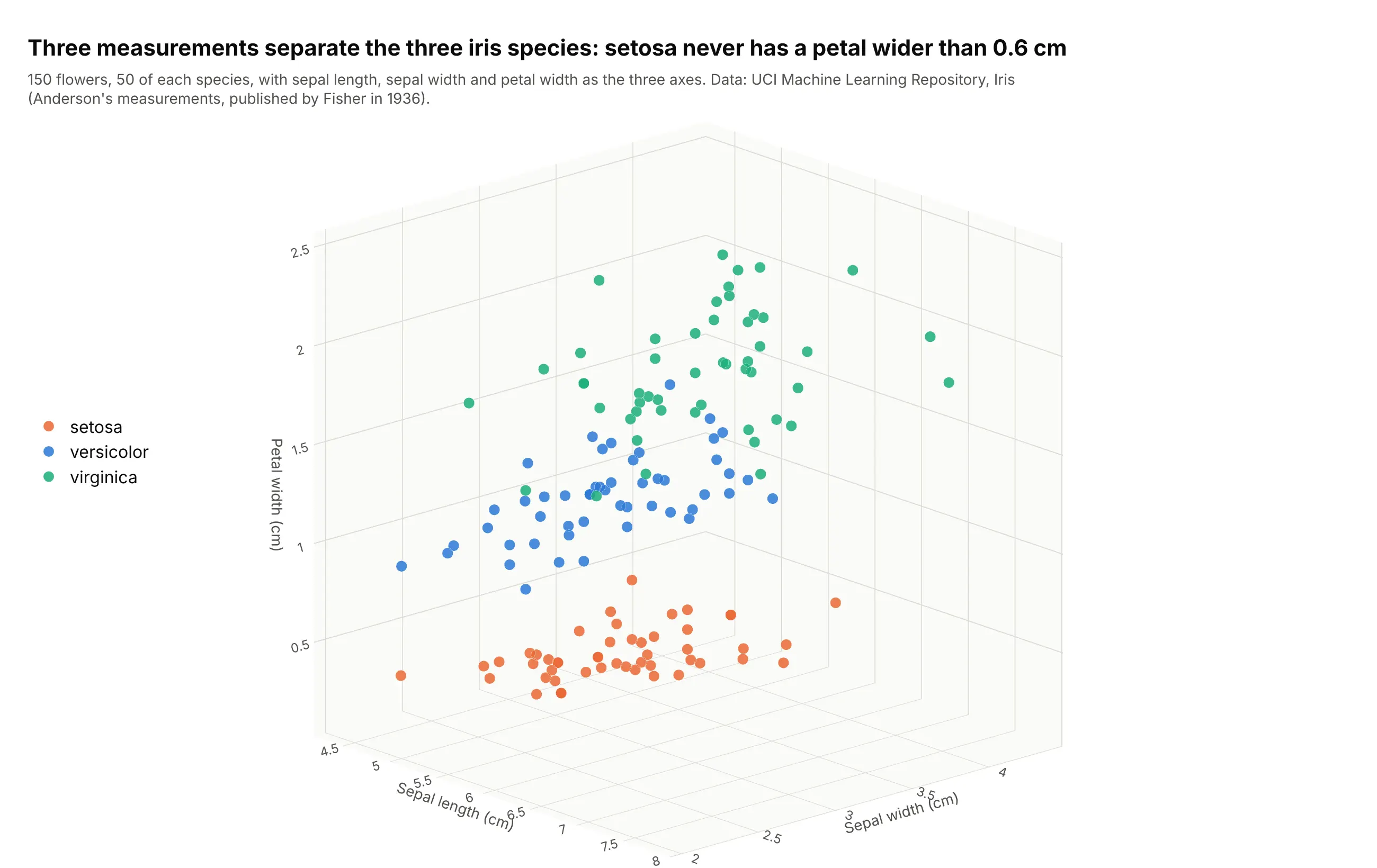
Three measurements on every sample, the classic textbook use. The iris data (150 flowers, three species) is the example in Plotly's own px.scatter_3d documentation and in MATLAB-style tutorials for scatter3: setosa never has a petal wider than 0.6 cm, while versicolor (1.0 to 1.8 cm) and virginica (1.4 to 2.5 cm) overlap between 1.4 and 1.8 cm. Data: UCI Machine Learning Repository, Iris (Fisher 1936).
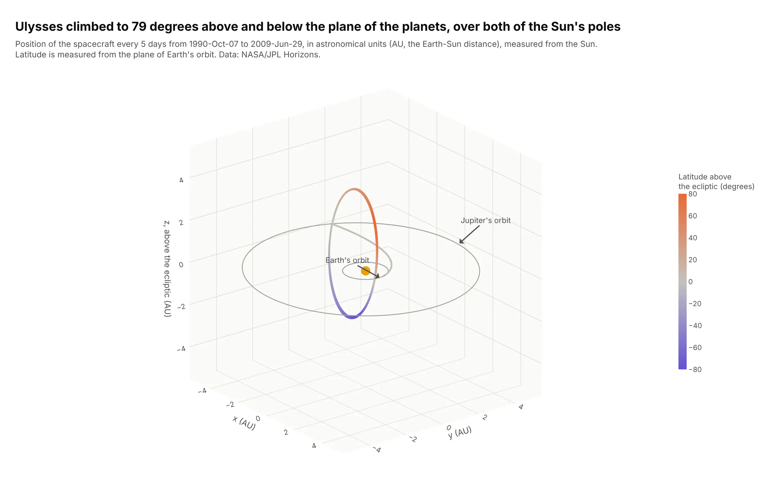
3D line charts of a trajectory. A 3D scatter plot with lines between the points in time order is a 3D line chart (MATLAB's plot3). The Ulysses spacecraft swung past Jupiter in 1992 to leave the plane of the planets, and it reached 79 degrees of latitude above that plane in 1995 and 79 degrees below it in 1994. Data: NASA/JPL Horizons system, one position every 5 days.
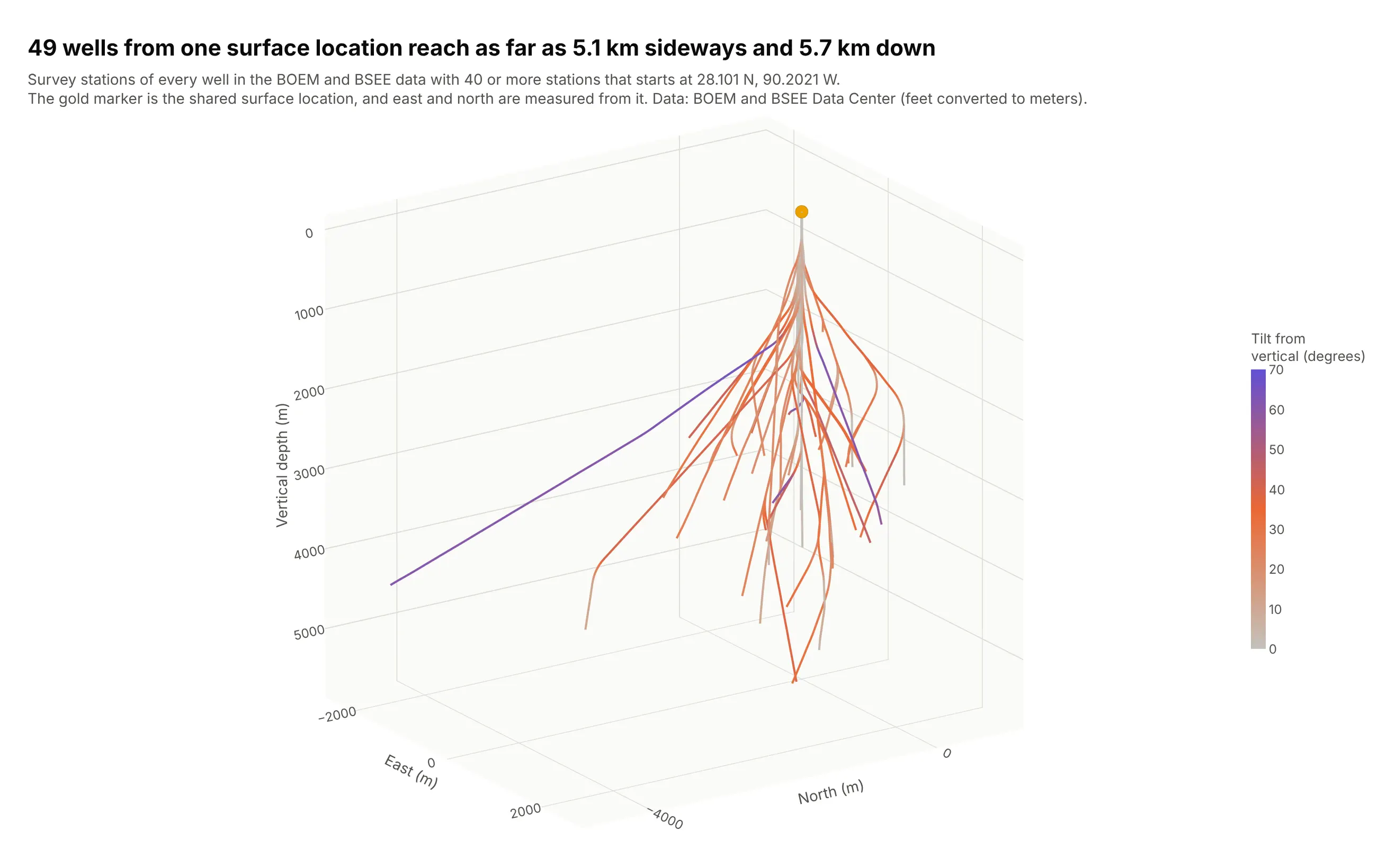
Well paths in 3D. Drillers steer wells sideways toward targets that are not straight below the platform, so each well is a 3D line through survey stations (a depth, an inclination and a direction measured along the hole). These 49 wells share one surface location and spread to a median of 953 m and a maximum of 5.1 km away, down to 5.7 km deep. Data: US Bureau of Ocean Energy Management (BOEM) and Bureau of Safety and Environmental Enforcement (BSEE) Data Center, directional survey points.
When 3D works and when it hurts
A 3D scatter plot has to squeeze three dimensions onto a flat screen, and that costs something. Three things go wrong, and they are the reason this guide recommends 2D alternatives for many cases.
Points hide each other. A point in front covers the points behind it, and a dense cloud turns into a blob from most angles. The same 5,099 earthquakes look very different from three angles:
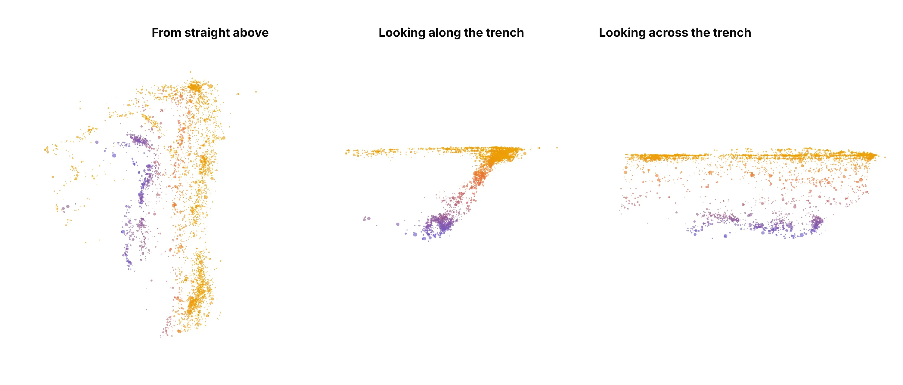
From above, depth disappears and the picture is a map. Looking along the trench (from the south) the slab appears as a tilted band that you can measure. Looking across the trench (from the east) the tilt disappears: the points spread out along the trench, and you see a shallow layer and a deep layer with a gap between them. A still image can only show one angle, so a published 3D scatter plot should be picked to show the structure the text talks about, or left interactive so readers can rotate it.
Distances are hard to compare. With perspective, which is Plotly's default camera, points that are farther away look smaller and closer together. Set scene_camera_projection_type="orthographic" (as every chart in this guide does) so equal distances are drawn equal. Even then, reading a coordinate off a 3D chart is much less precise than reading it off a 2D axis. In a set of experiments by Tory and colleagues (2006), 3D displays were effective for approximate positioning when cues such as shadows were present, but "not effective for precise navigation and positioning", and views that combined 2D and 3D worked as well or better.
A still image loses the main benefit. Depth in a 3D scatter plot comes mostly from motion. In an experiment by Sollenberger and Milgram (1993) rotating displays beat flat ones in tracing a 3D path, and they beat stereoscopic ones too. So use a 3D scatter plot where readers can drag it, and for a static page or a PDF, prefer a 2D chart or show two or three 2D views next to each other.
When does 3D earn its place? When the three axes are physical dimensions, as with earthquake depth, a drill path or a map of stars, or when the question is about the shape of a cloud, such as clusters, a tilted sheet or an outlier far from the rest. When the third variable is a measurement (a price, a score, a concentration), color or marker size on a 2D scatter plot usually says the same thing more clearly.
A short history
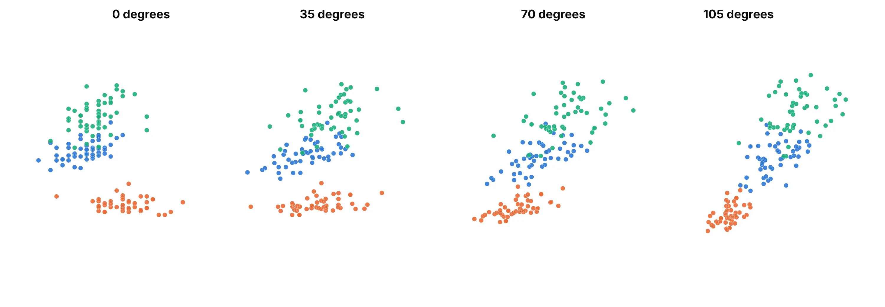
Rotating a cloud of points to see its depth goes back to the first interactive graphics systems. In April 1974, Mary Anne Fisherkeller, Jerome Friedman and John Tukey at the Stanford Linear Accelerator Center described PRIM-9, a system whose operator could rotate a point cloud in real time. Their report explains that "from the parallax effect, arising from the dynamic aspect of this continuous rotation, one perceives a third dimension (depth into the screen)", and the system handled data in up to nine dimensions. Here is that idea redrawn: the same cloud of iris flowers (not PRIM-9's own data, which we don't have) at four angles, where the apparent positions of the three groups shift from view to view, which is how the eye reads depth from rotation:
The tools most people use today came later: MATLAB's scatter3 ("3-D scatter plot") and plot3 ("3-D line plot") are both listed as introduced before R2006a, matplotlib's Axes3D.scatter draws a static 3D scatter plot, and the R package scatterplot3d "plots a three dimensional (3D) point cloud". Plotly's scatter3d trace, drawn with WebGL (the browser's graphics interface), made the same chart interactive in a web page.
Alternatives to a 3D scatter plot
Here are the same Tonga earthquakes drawn six ways. Some are better for the question, some worse, some just different:
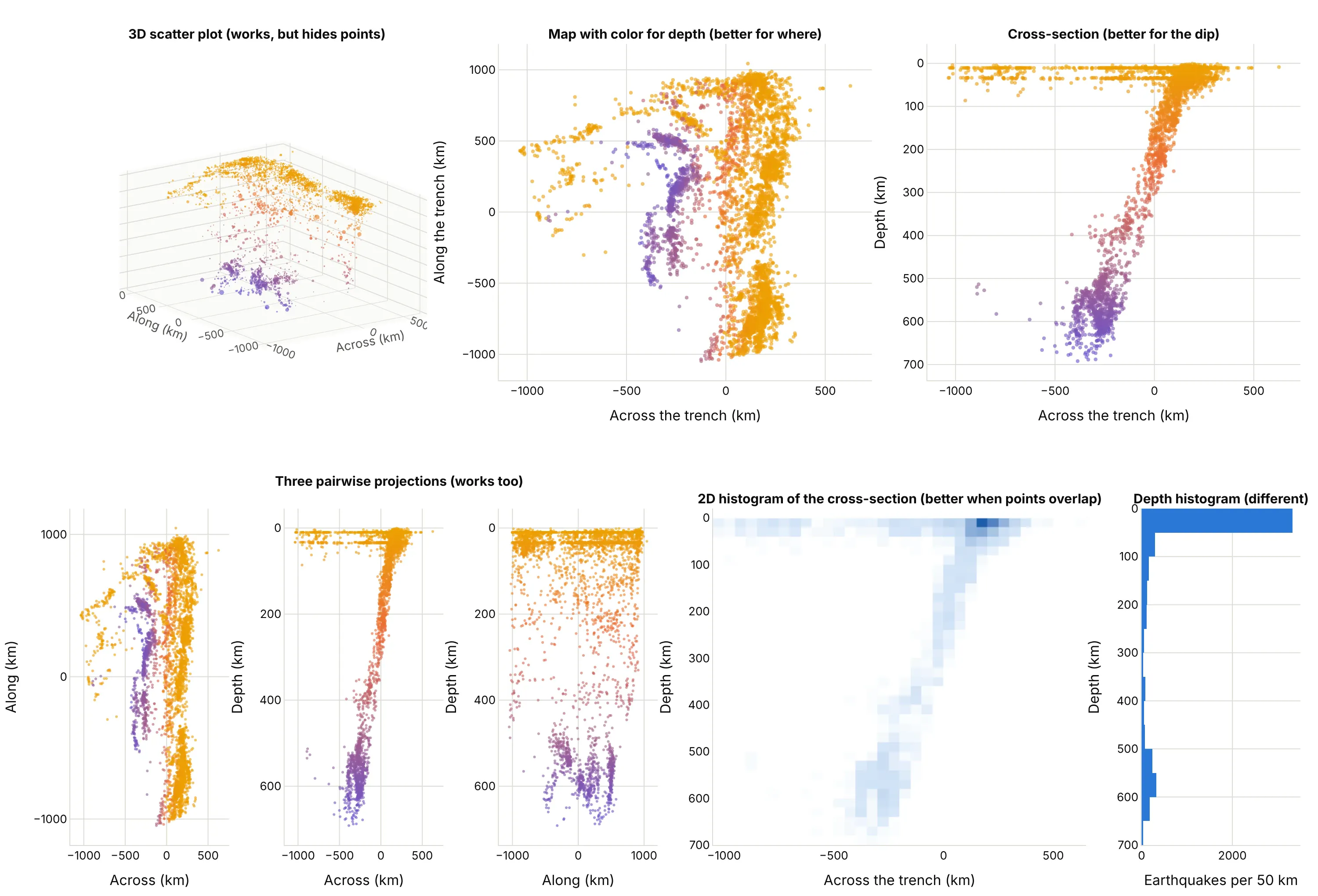
- Scatter plot with color for the third variable (better for where). The map view shows the position of every earthquake exactly, and the color gives the depth. You lose the sense of a surface, but the position and the depth both read off without rotating.
- A 2D cross-section (better for the dip). Plotting depth against the distance across the trench makes the slab a clear diagonal line you can measure. When you know which two variables matter most, this beats any 3D angle. It is also how seismologists draw it.
- Pairwise projections, or a scatter plot matrix (works too). One flat scatter plot for each pair of variables, so every coordinate reads off an axis. You need to combine the panels in your head, which gets hard with many variables, but it never hides points behind other points.
- 2D histogram or heatmap (better when points overlap). With thousands of points, counting them in cells shows where they pile up instead of drawing every marker on top of the last one.
- Bubble chart (different). A 2D scatter plot with marker size for the third variable. It fits a measurement better than a coordinate, at the cost of less precise reading.
- Small multiples (works too). A grid of 2D charts, one for each slice (for example, one map for each depth range), which keeps every point visible and the same scale.
- 3D surface plot (different). When z is a function of x and y on a grid, such as terrain or a risk surface, a surface shows it as a sheet; a 3D scatter plot is for points that don't sit on a grid. For counts in a grid, a 3D bar chart is the 3D relative.
- Isosurface or volume plot (different). When you measured a quantity everywhere in space (temperature in a room), draw the field itself and not a point for each sample.
For a 3D line chart, the flat alternatives are three line charts of x, y and z against time, or a map view with color for time. A 3D line is worth keeping when the path itself is the object, as in the Ulysses and well examples.
How to make a 3D scatter plot
With AI
ChatGPT, Claude Code, GitHub Copilot, Cursor and other AI tools are excellent at writing Plotly code. Name Plotly in the prompt, and say what the axes mean, because the defaults (a cube, a perspective camera, a depth axis that runs upward) are wrong for most real data:
Make a plotly 3D scatter plot from quakes.csv (columns: across_km, along_km, depth_km, mag, time, place).- px.scatter_3d with x=across_km, y=along_km, z=depth_km, marker size from mag and color from depth_km.- Flip the depth axis so deeper is lower, use scene aspectmode "data" so kilometers have the same length on every axis,and an orthographic camera.- Axis titles with units, 0.7 opacity, a hover label with time, magnitude and depth, and a title that statesthe takeaway. Then also show a 2D cross-section of depth against across_km next to it.
With Plotly Studio
Plotly Studio is a product for creating data visualizations and Dash apps and for analyzing data with AI, available as a desktop app or embedded in Dash apps. Ask for a 3D scatter plot the same way:
Plot these earthquakes as a 3D scatter plot of longitude, latitude and depth with the depth axis flipped, marker size by magnitude, a year slider, and a 2D map view of the same points next to it.
Make a 3D scatter plot in Python or JavaScript
This is the code AI tools write under the hood. In Python, px.scatter_3d takes a table and the names of three columns:
import pandas as pdimport plotly.express as pxdf = pd.read_csv("quakes.csv") # columns: across_km, along_km, depth_km, mag, time, placefig = px.scatter_3d(df, x="across_km", y="along_km", z="depth_km", color="depth_km", size="mag",size_max=10, opacity=0.7, hover_name="place",labels={"across_km": "Across the trench (km)", "along_km": "Along the trench (km)", "depth_km": "Depth (km)"})fig.update_scenes(zaxis_autorange="reversed", aspectmode="data")fig.update_layout(scene_camera_projection_type="orthographic")fig.show()
go.Scatter3d gives you every option, and mode="lines" turns the same data into a 3D line chart. This one draws a spacecraft path and colors it by latitude:
import numpy as npimport pandas as pdimport plotly.graph_objects as godf = pd.read_csv("ulysses.csv") # columns: date, x, y, z in astronomical units (AU), from the Sundf["latitude"] = np.degrees(np.arcsin(df.z / np.sqrt(df.x**2 + df.y**2 + df.z**2)))fig = go.Figure(go.Scatter3d(x=df.x, y=df.y, z=df.z, mode="lines",line=dict(width=6, color=df.latitude, colorscale="Portland", colorbar=dict(title="Latitude")),text=df.date, hoverinfo="text"))fig.update_layout(scene=dict(aspectmode="cube", camera=dict(projection=dict(type="orthographic"))))fig.show()
If you're coming from matplotlib, ax.scatter(x, y, z) on a projection="3d" axis maps to px.scatter_3d(x=, y=, z=), and ax.plot(x, y, z) to mode="lines"; the difference is that matplotlib draws a static image, while the Plotly chart rotates, zooms and shows a hover label for each point. MATLAB's scatter3(X, Y, Z, S, C) corresponds to size (S) and color (C), and plot3(X, Y, Z) to mode="lines".
In JavaScript, plotly.js draws the same chart from a scatter3d trace. This example plots the 12 largest earthquakes in the Tonga data:
<div id="chart"></div><script src="https://cdn.plot.ly/plotly-4.1.1.min.js"></script><script>// The 12 largest earthquakes in the USGS catalog under Tonga and Fiji, 2000 to 2025const across = [-254, 271, 165, 204, -491, 35, -286, -421, 233, 252, 37, 24];const along = [491, 932, -725, 377, 387, -334, 73, -214, 57, -681, 854, -1002];const depth = [600, 18, 29, 55, 671, 152, 580, 675, 31, 17, 210, 152];const mag = [8.2, 8.1, 8.1, 8.0, 7.9, 7.8, 7.7, 7.7, 7.6, 7.6, 7.6, 7.4];Plotly.newPlot("chart", [{type: "scatter3d", mode: "markers", x: across, y: along, z: depth,text: mag.map((m, i) => `M${m}, ${depth[i]} km deep`), hoverinfo: "text",marker: {size: mag.map(m => (m - 6.5) * 6), color: depth, colorscale: "Portland", opacity: 0.8,colorbar: {title: {text: "Depth (km)"}}}}], {width: 800, height: 600,scene: {xaxis: {title: {text: "Across the trench (km)"}}, yaxis: {title: {text: "Along the trench (km)"}},zaxis: {title: {text: "Depth (km)"}, autorange: "reversed"},aspectmode: "data", camera: {projection: {type: "orthographic"}}}});</script>
Share it
Every Plotly chart has a Share chart button (the cloud icon in its toolbar) that uploads it to Plotly Cloud and gives you a link. Only you can see it until you change its visibility.
For a live app, put the chart in a Dash app and publish it with the Plotly Cloud command-line interface (CLI). Coding agents can run these commands for you:
pip install "dash[cloud]"plotly user loginplotly app publish
If your data has to stay in your own cloud or data center, publish to Dash Enterprise instead.
Dos and don'ts
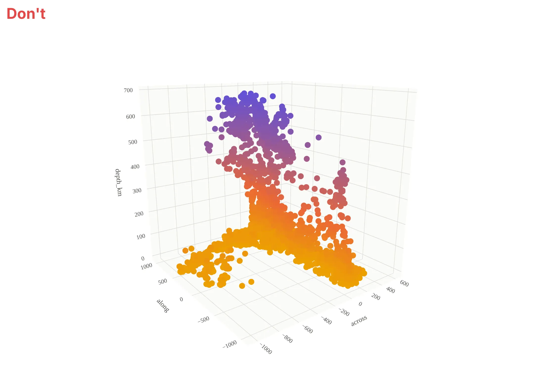
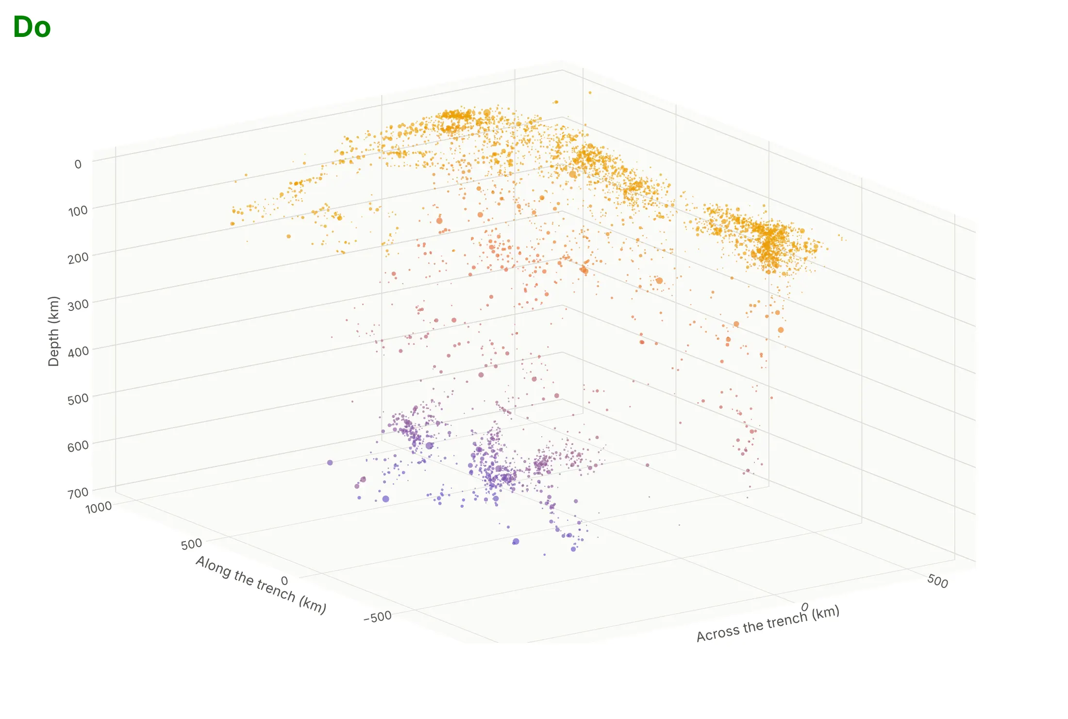
Most of what goes wrong with a 3D scatter plot is about geometry and overlap, so the fixes are about axes, camera and markers. Here are the Tonga earthquakes both ways, in the same colors.
Don't leave the depth axis running upward so that deeper earthquakes appear higher, accept the default cube that squeezes kilometers into a shape that isn't the real one, draw every earthquake as the same large opaque marker so they cover each other, leave the column names as axis titles with no units, keep the default perspective camera and use a serif font:
Do flip the depth axis, set the box proportions from the data (here depth is stretched 1.5 times, and the main chart says so), size the markers by magnitude and make them slightly transparent, name the axes in words and units, and use an orthographic camera at an angle that shows the slab's tilt:
Checklist
Do
- Make the three axes physical dimensions, or the question about a cloud's shape; otherwise use color or size on a 2D chart.
- Use an orthographic camera so equal values look equal, and set aspectmode="data" when all axes share a unit (or stretch one axis on purpose and say so).
- Flip the axis (autorange="reversed") when the variable is depth.
- Make markers small and a little transparent (opacity 0.6 to 0.8), and put the points of each group in one trace, never one trace per point.
- Leave the chart interactive, and for a still image choose the camera angle that shows what the text says.
- Add hover text with the exact values, because coordinates are hard to read off a 3D axis.
- Show a 2D view (a cross-section, a map or a scatter plot matrix) when exact positions matter.
Don't
- Use 3D for two variables; a flat scatter plot says the same thing more clearly.
- Publish a still 3D image where points hide the ones you discuss.
- Encode a measurement (price, score) as z when color on a 2D scatter plot would do.
- Draw one trace per point or one trace per row; it is many times slower than one trace per group.
- Mix units (kilometers against degrees) on axes that share a box without setting the proportions.
More 3D scatter plot examples
Six more 3D scatter plots and 3D line charts built from real public data, each with its source, the technique that makes it work and a prompt to rebuild it.
1. Wine chemistry as three principal components
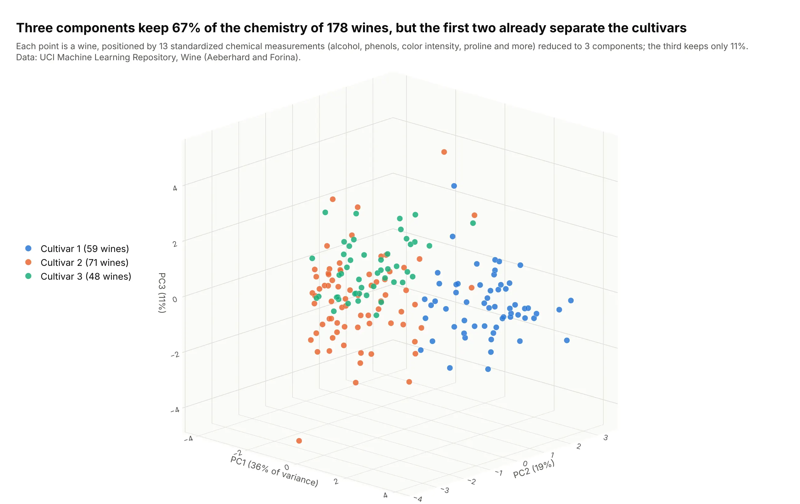
Principal component analysis (PCA) turns 13 chemical measurements of 178 wines into new axes that keep as much of the variation as possible; the first three keep 67% (36%, 19% and 11%). The first two components already pull the three cultivars apart (cultivar 1 averages 2.3 on PC1, cultivar 3 averages -2.8), and the third adds little, which a 3D view can't make obvious. Data: UCI Machine Learning Repository, Wine (Aeberhard and Forina).
Tip: standardize each measurement before PCA, otherwise proline (hundreds) outweighs hue (about one).
Get the data from the UCI Machine Learning Repository wine data set (wine.data: 178 rows, the first column is thecultivar 1 to 3, then 13 chemical measurements such as alcohol, flavanoids, color intensity and proline).Standardize the 13 measurements, run a 3-component PCA with scikit-learn, and make a plotly px.scatter_3d of thecomponents colored by cultivar, with the share of variance in each axis title, an orthographic camera and atitle that says what the components separate.
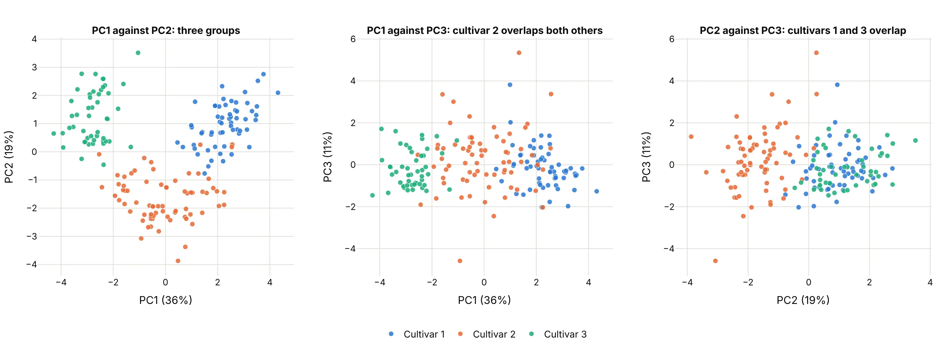
Another way to see it: the three 2D projections of the same components. The first panel (PC1 against PC2) shows three groups, while the panels with PC3 overlap more (cultivar 2 overlaps both others against PC1, and cultivars 1 and 3 overlap against PC2), so the third axis adds little and costs some occlusion:
2. Industries on the three Fama/French factors
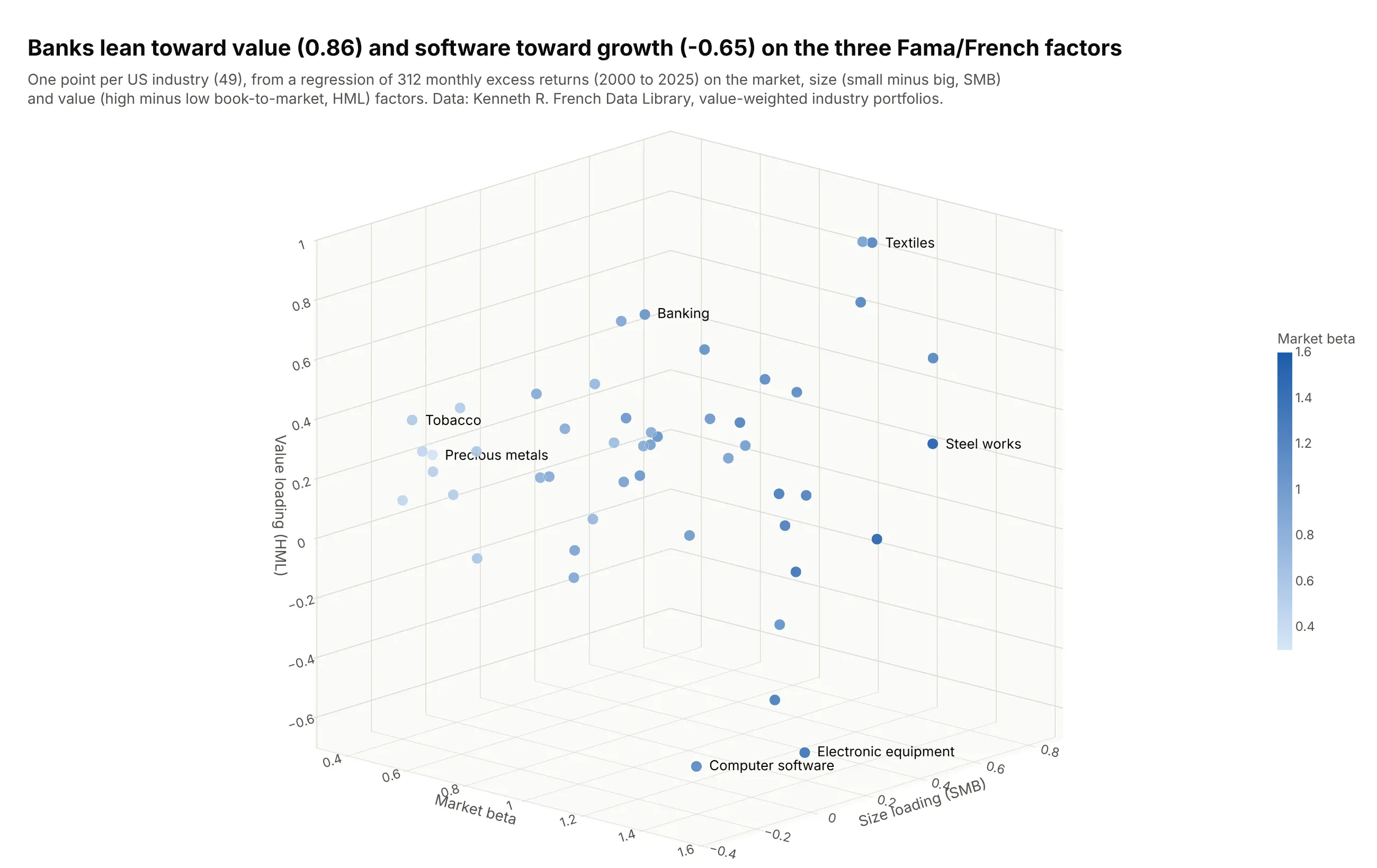
The Fama/French model explains stock returns with three factors: the market, size (small companies minus big ones, SMB) and value (cheap minus expensive companies by book-to-market ratio, HML). Regressing 312 monthly returns on them places each industry at three loadings: banking has a value loading of 0.86 and computer software has -0.65, while precious metals have a market beta of just 0.33 against 1.59 for steel works. Data: Kenneth R. French Data Library, value-weighted returns of 49 industry portfolios, January 2000 to December 2025.
Tip: label only the extremes; a label on every one of 49 points covers the points.
Get the data from the Kenneth R. French Data Library: the monthly value-weighted returns of the 49 industry portfoliosand the Fama/French 3 factors (Mkt-RF, SMB, HML, RF), January 2000 to December 2025.For each industry regress the excess return (industry minus RF) on the three factors with numpy least squares, and makea plotly px.scatter_3d of the three loadings, with the market beta as the color, text labels only for the industrieswith the most extreme loadings, an orthographic camera and a title with the highest and lowest value loadings.
3. The Sun's neighborhood in 3D
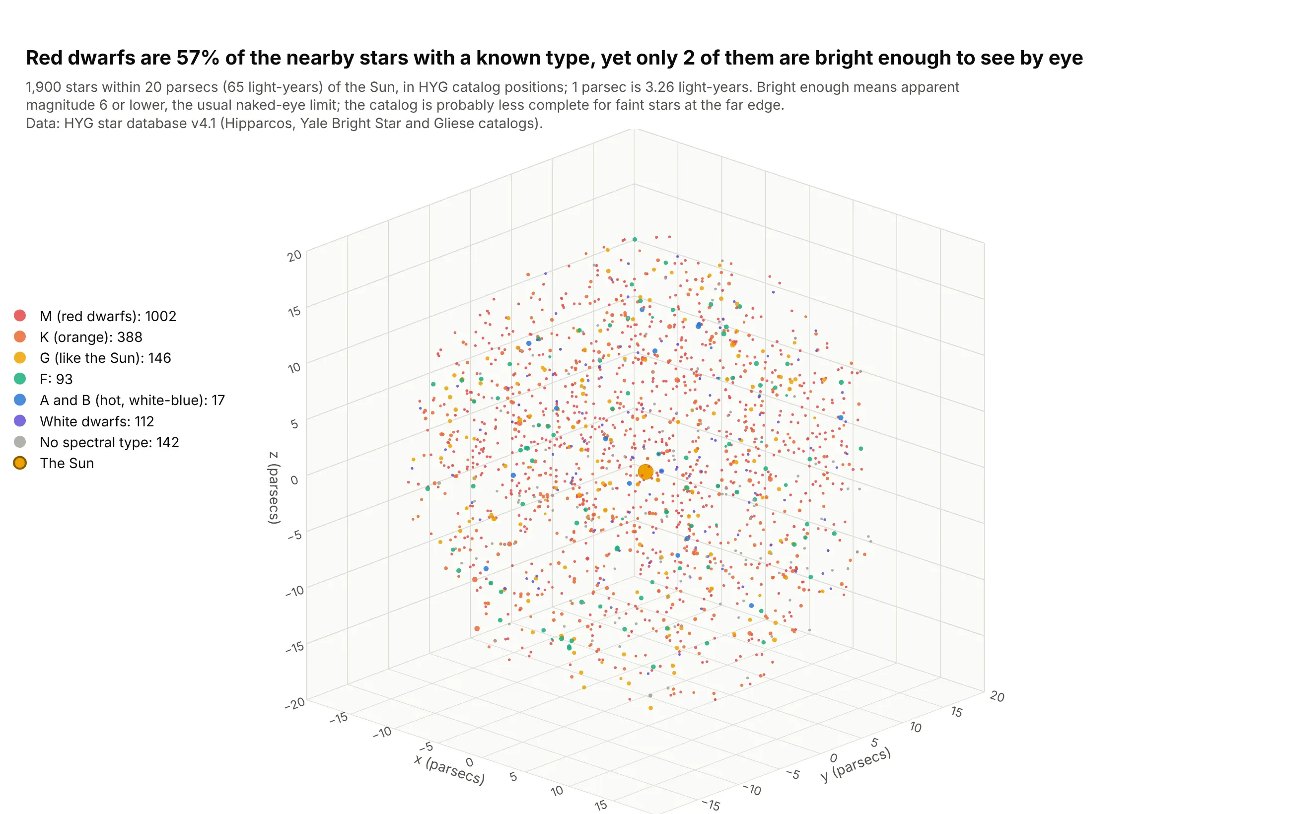
The 1,900 stars within 20 parsecs (65 light-years) of the Sun in this catalog are mostly red dwarfs: they make up 57% of the 1,758 with a spectral type, yet only 2 of them are bright enough to see without a telescope (apparent magnitude 6 or lower), against 224 stars of all types. All three axes are in parsecs, so a cube is the honest shape. Data: HYG star database v4.1, which combines the Hipparcos, Yale Bright Star and Gliese catalogs.
Tip: when the axes share a unit and no direction is special, use aspectmode="cube" and draw a reference point such as the Sun.
Get the data from the HYG star database v4.1 (hygdata_v41.csv on GitHub, astronexus/HYG-Database): keep stars withdist <= 20 parsecs, excluding the Sun (columns: proper, dist, x, y, z, mag, absmag, spect).Make a plotly 3D scatter plot of x, y, z with one trace for each spectral class taken from the first letter ofspect (M, K, G, F, A and B, D for white dwarfs), marker size from absmag, the Sun as a gold marker at the origin, acube aspect mode and an orthographic camera.
4. A glider's dives through the Caribbean
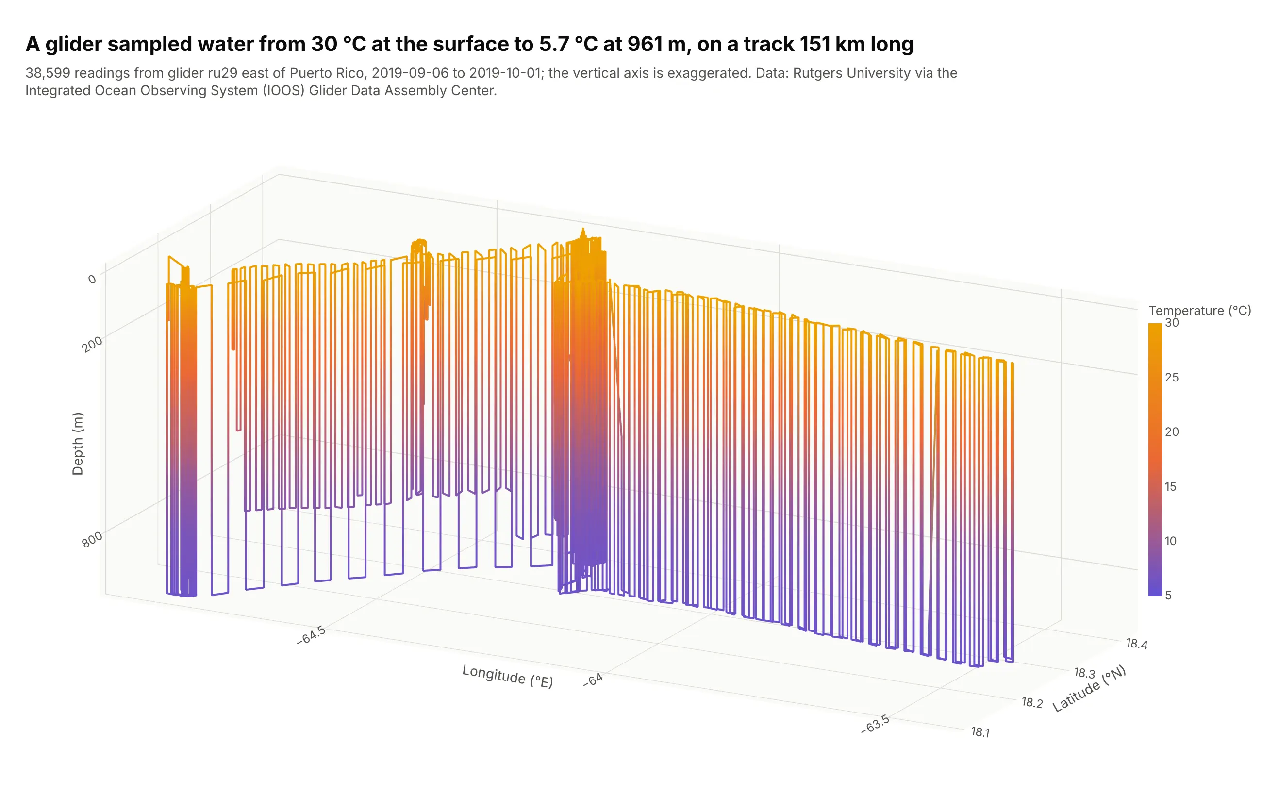
A Rutgers University glider is an autonomous underwater vehicle that zigzags between the surface and about 1,000 m as it travels. This 25-day mission covers about 151 km east to west and 38,599 readings, with water from 30.1 °C at the surface to 5.7 °C at 961 m, so the line colored by temperature shows the warm layer on top and the cold water below. Data: Rutgers University glider ru29, deployment ru29-20190906T1535, via the Integrated Ocean Observing System (IOOS) Glider Data Assembly Center; the dataset notes say the data may be redistributed and used without restriction.
Tip: exaggerate the vertical axis for tracks that are wide and shallow; a true-scale box would squash a 961 m dive against 151 km of travel into a flat line.
Get the data from the IOOS Glider Data Assembly Center ERDDAP server (gliders.ioos.us/erddap), datasetru29-20190906T1535, as CSV (columns: time, latitude, longitude, depth, temperature, salinity).Make a plotly go.Scatter3d with mode="lines" of longitude, latitude and depth with the depth axis flipped and theline colored by temperature, a manual aspect ratio that exaggerates the vertical axis, and a hover label with time,depth and temperature.
5. 100,000 galaxies
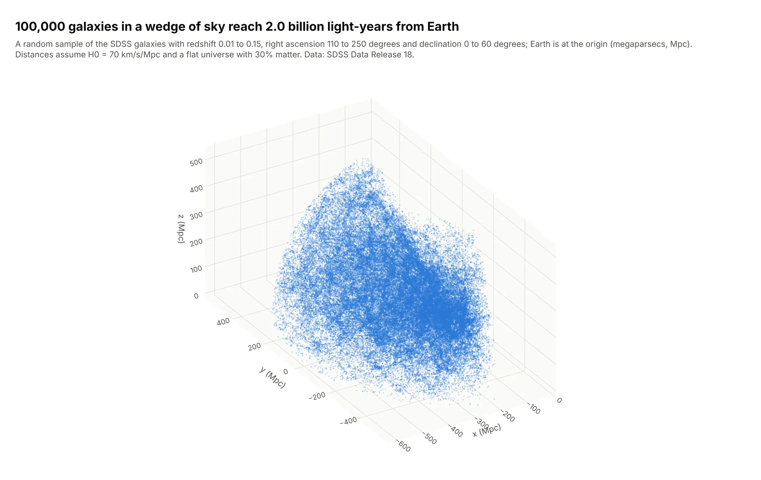
A galaxy survey is a literal 3D map: a sky position and a redshift (how far the light has been stretched, which gives distance) become coordinates in megaparsecs. This sample of 100,000 of the 473,601 galaxies the query returned reaches 620 Mpc, or 2.0 billion light-years, and draws as one WebGL trace. The density thins with distance, probably because a survey only catches the brighter galaxies far away (our reading, not a measurement). Data: Sloan Digital Sky Survey (SDSS) Data Release 18, SpecObj table, redshift 0.01 to 0.15, right ascension 110 to 250 degrees and declination 0 to 60 degrees.
Tip: at this size use size of 1 to 2 pixels and an opacity near 0.3 so dense regions build up instead of saturating.
Get the data from the Sloan Digital Sky Survey DR18 SkyServer SQL search (SpecObj table: class = 'GALAXY',zWarning = 0, sciencePrimary = 1, z between 0.01 and 0.15, ra between 110 and 250, dec between 0 and 60), columns ra, dec, z.Convert the redshift to a comoving distance in Mpc for H0 = 70 and a flat universe with 30% matter, then to x, y, zfrom ra and dec, and make a plotly go.Scatter3d of a 100,000 galaxy random sample with 1.3 pixel markers at 0.28opacity, equal axes and an orthographic camera.
6. A drug bound to its target protein
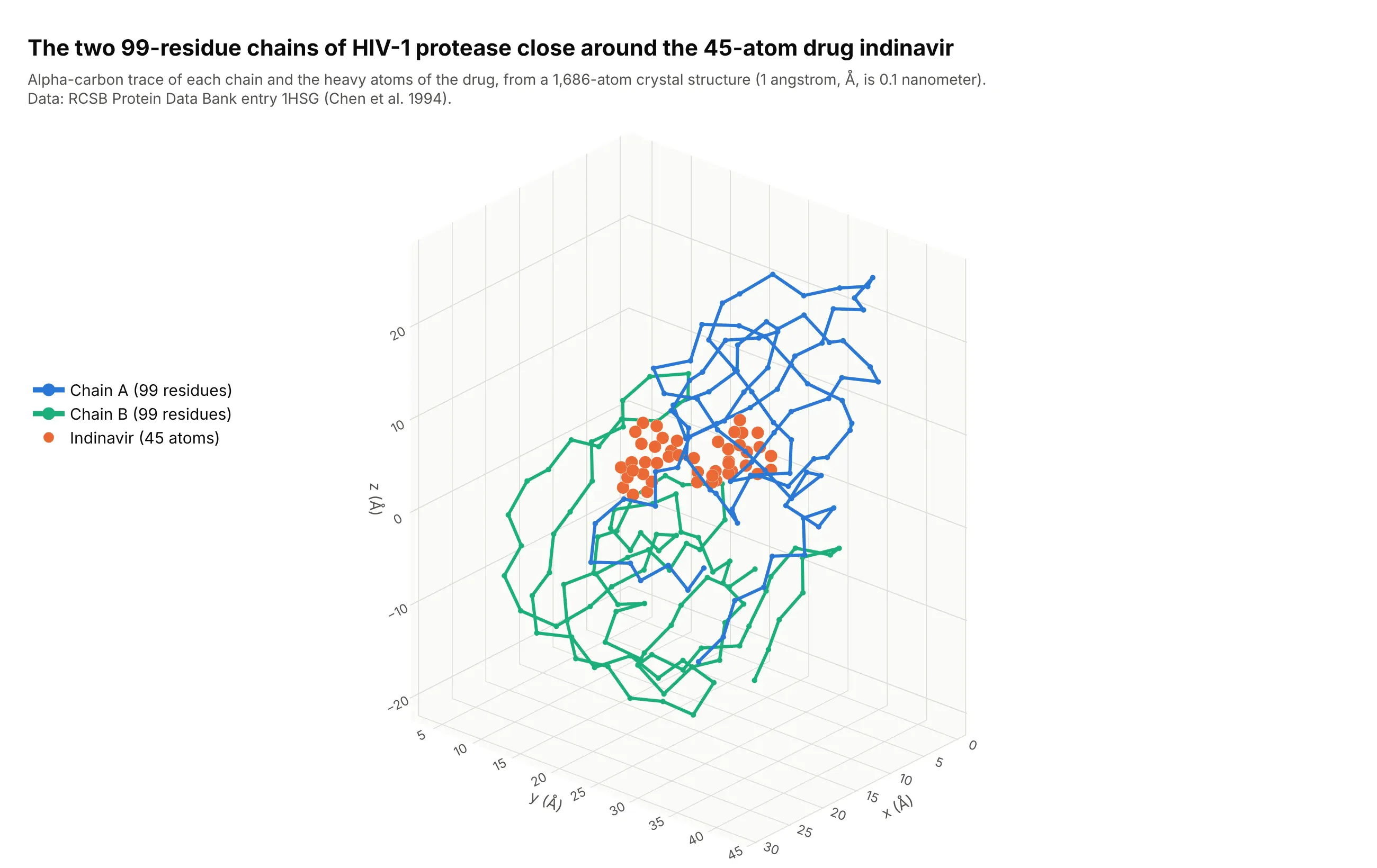
A crystal structure is a list of atoms with x, y and z coordinates in angstroms (Å, a tenth of a nanometer), which makes it a point cloud by nature. This entry, 1HSG, has 1,686 atoms: 99 residues in each of the two chains of HIV-1 protease, and the 45 heavy atoms (36 carbon, 5 nitrogen and 4 oxygen) of the drug indinavir. Drawing a line through each chain's alpha carbons shows how it folds around the drug. Data: RCSB Protein Data Bank entry 1HSG, Chen et al. (1994), Journal of Biological Chemistry 269, 26344.
Tip: draw the backbone as lines+markers on the alpha carbons only; drawing all 1,514 protein atoms hides the drug.
Get the data from the RCSB Protein Data Bank entry 1HSG (files.rcsb.org/download/1HSG.pdb): parse the ATOM and HETATMlines into columns record, atom name, residue, chain, residue number, x, y, z.Make a plotly 3D chart with one go.Scatter3d of mode "lines+markers" through the alpha carbons (atom name CA) ofeach chain in a different color, one go.Scatter3d of markers for the ligand MK1 in orange, axes in angstroms withequal scale, and an orthographic camera.
FAQ
Options to customize
A 3D scatter plot in Plotly is a scatter3d trace inside a 3D scene, so these are the options that matter most. The full lists are in the scatter3d trace reference and the 3D scene layout reference.
- x, y, z: the coordinates of each point; one array per axis (or column names in px.scatter_3d).
- mode: "markers", "lines", "text" or a combination joined with +; "lines" makes a 3D line chart, and the default is "lines+markers".
- marker.size and marker.sizemode: marker size in pixels (a single number or an array for a fourth variable); sizemode is "diameter" or "area". In px.scatter_3d, use size and size_max.
- marker.color, marker.colorscale, cmin and cmax: color by value on a color scale, and fix the range so several charts share one scale.
- marker.opacity and marker.line: transparency so dense clouds show their density, and a thin white outline so overlapping markers stay distinct.
- marker.symbol: one of the eight 3D symbols (circle, circle-open, cross, diamond, diamond-open, square, square-open, x), for a category.
- line.width, line.color and line.dash: width, color (a single color or an array to color along the line) and dash style for 3D lines.
- text, hovertext and hoverinfo: the label for each point on hover, and text with mode="text" for permanent labels.
- error_x, error_y and error_z: error bars along each axis.
- projection (with x, y and z): draws the shadow of the points or line on the walls of the scene.
- scene.camera.projection.type: "orthographic" draws equal distances at equal sizes; the default is "perspective".
- scene.camera.eye, center and up: where the camera stands, what it looks at and which way is up.
- scene.aspectmode and aspectratio: "data" for true proportions, "cube" for equal lengths, "manual" with a ratio of your choice.
- scene.zaxis.autorange="reversed": flips an axis, which is how you draw depth.
- scene.xaxis.range, type="log" and tickvals: set limits, use a log scale or place your own ticks on any 3D axis.
- px.scatter_3d parameters color, size, symbol, animation_frame and hover_name: the Plotly Express shortcuts that make one trace per group and wire the legend.