Isosurface and Volume Plots - A Complete Guide

TL;DR

• An isosurface plot draws the surface where a 3D scalar field (a number measured at every point in space, such as the temperature of the ocean at every longitude, latitude and depth) equals one chosen value, the 3D version of a contour line. A volume plot stacks many translucent isosurfaces so the field reads like a cloud.
• Isosurfaces are also known as level sets, and are similar to contour plots, 3D surface plots, image plots with imshow and vector field plots.
• Use one when the shape of a boundary in 3D is the finding: a thermocline, a jet stream, a molecular orbital, a metal part in a computed tomography (CT) scan or a channel of sand in a reservoir. Use slices or contours when readers need the exact values.
• You can make both with Plotly in Python or JavaScript, from go.Isosurface and go.Volume, and draw slices through the same cube. Both take a flat list of x, y, z positions and one value per position, and run in the browser with WebGL.
• Plotly draws a few hundred thousand cells smoothly. For a bigger scan, compute the surface once with marching cubes and draw it as go.Mesh3d, as the FAQ measures below.

What is an isosurface plot?

Isosurface plots look like this:

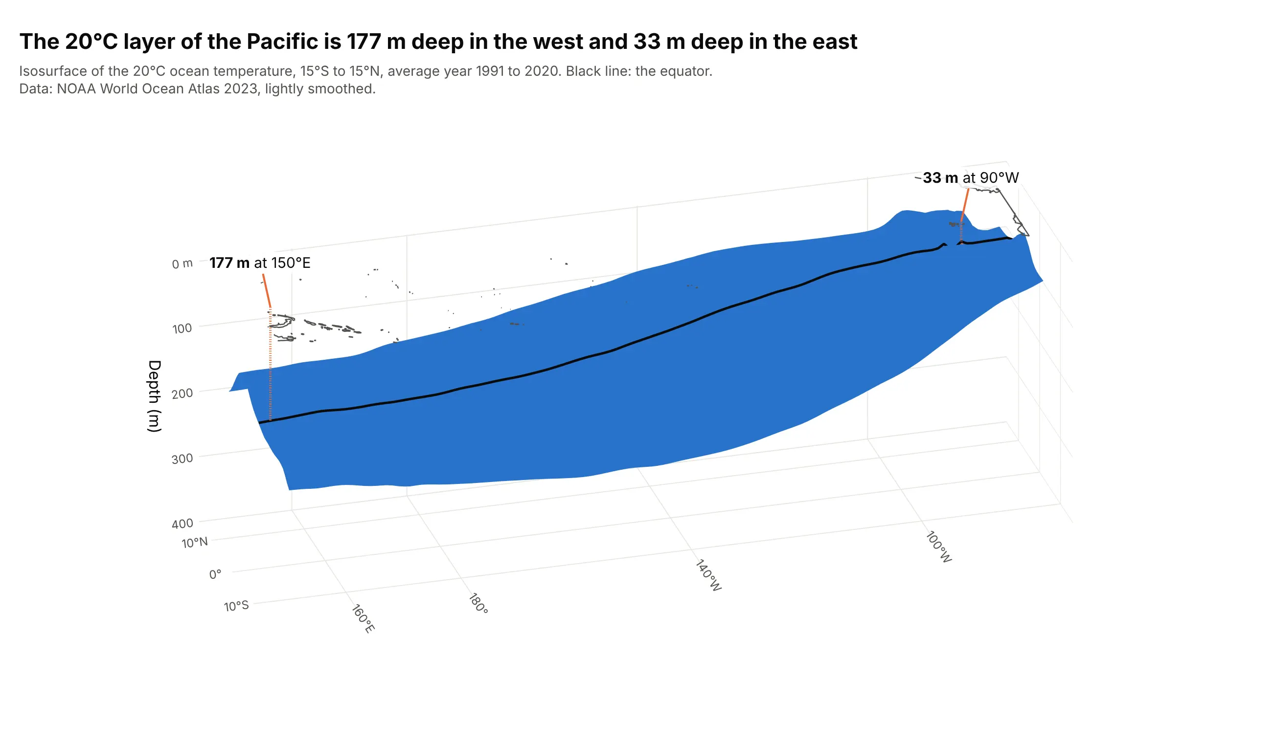
Data: National Oceanic and Atmospheric Administration (NOAA) World Ocean Atlas 2023, annual mean temperature for 1991 to 2020 on a 1 degree grid, 132 x 30 x 37 cells. Land and sea-floor cells are filled with the nearest ocean value, and the cube is interpolated to 5 m depth steps and lightly smoothed (Gaussian filter) so the surface is one smooth sheet. The depths quoted below come from the unsmoothed data.

A 3D scalar field is a number at every point of a 3D grid, here the temperature at each longitude, latitude and depth. An iso-value is one chosen number from that field, and the isosurface is every place where the field equals it, in the same way a contour line on a map joins every place with the same elevation. How do you read an isosurface plot? In the example above, notice these things:

• Every point on the blue sheet is exactly 20°C. Water above it is warmer and water below it is colder, so the sheet is a boundary and not a thing.
• Position carries the data. The sheet's depth, read on the vertical axis, is the depth of the 20°C layer, which sits at 177 m at 150°E and 33 m at 90°W along the equator.
• That 144 m tilt across the basin is the tilt of the ocean's thermocline, the transition layer between warm surface water and cold deep water. NOAA describes the thermocline this way, and its Climate Prediction Center publishes the depth of the 20°C isotherm as a routine monitoring product.
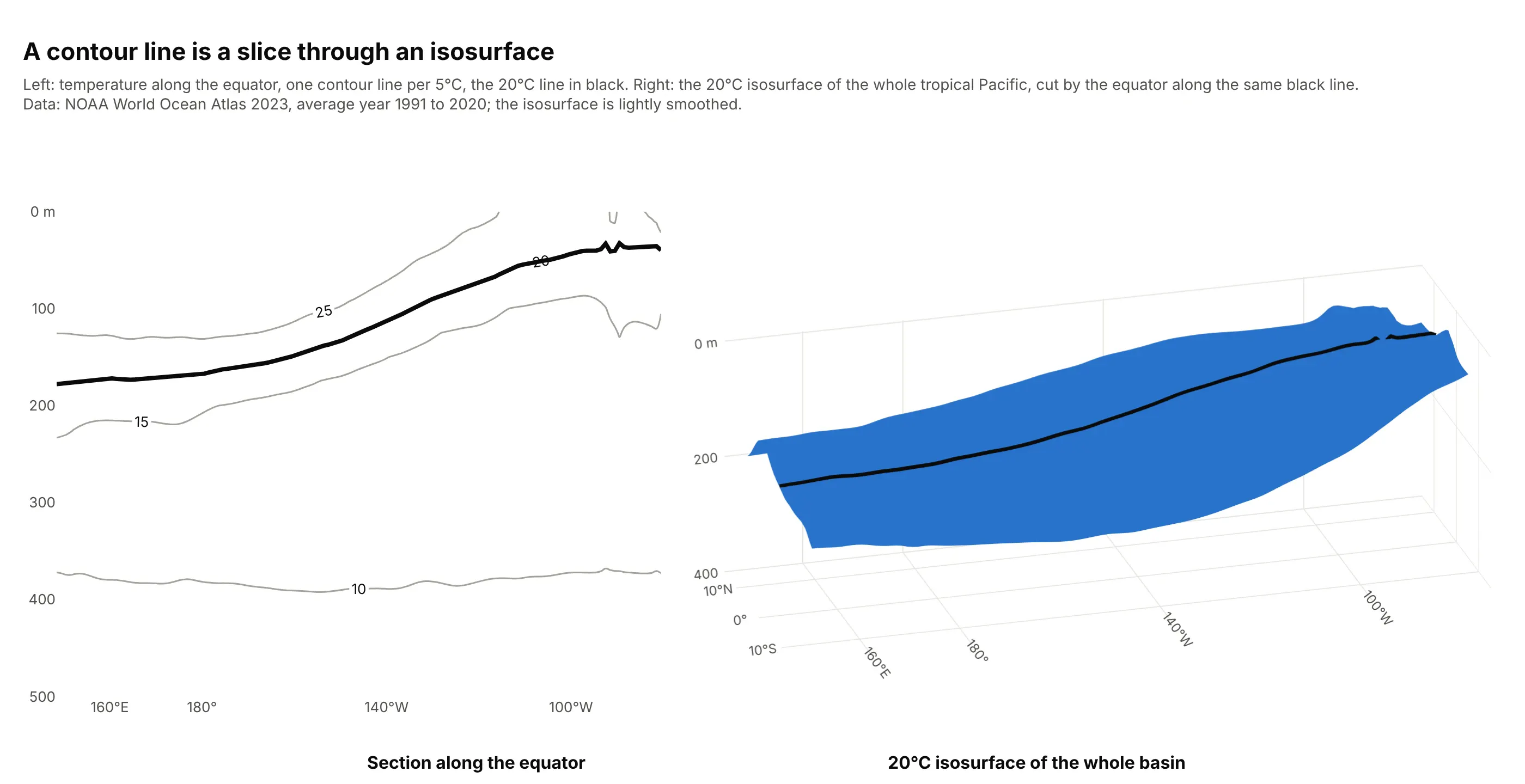
• The black line is where the equator's vertical section cuts the surface. It is the same 20°C contour line you would draw on a 2D section, which is how an isosurface relates to a contour plot.

It's often used for charts like these:

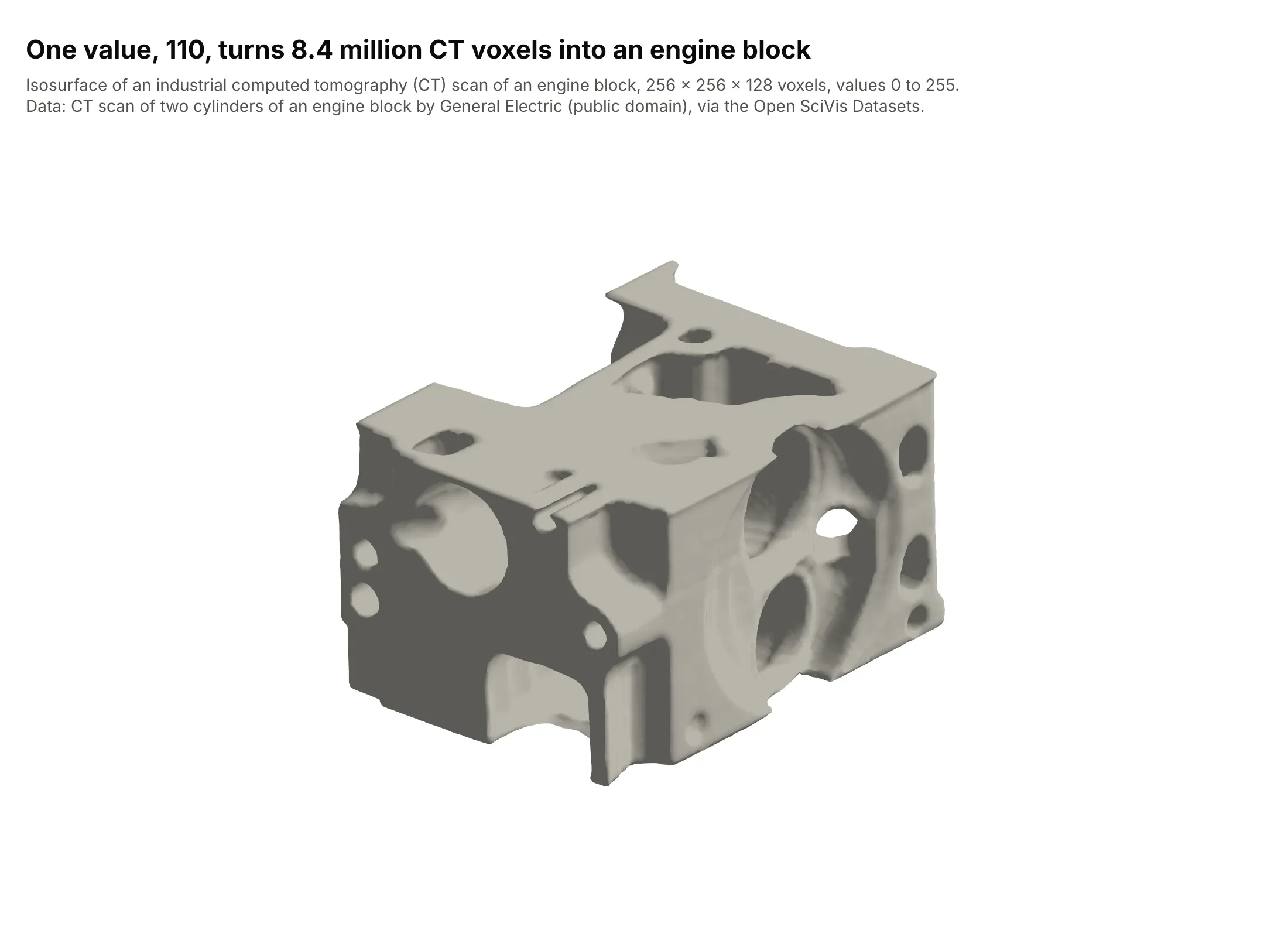
Engineering inspection. One value, 110, turns 8.4 million CT voxels into an engine block, with its bores, ports and bolt holes. Marching cubes was introduced for medical scans, and industrial scans of castings and printed parts use the same method. Data: CT scan of two cylinders of an engine block, General Electric (public domain), 256 x 256 x 128 voxels, via the Open SciVis Datasets and the Stanford volume data archive.

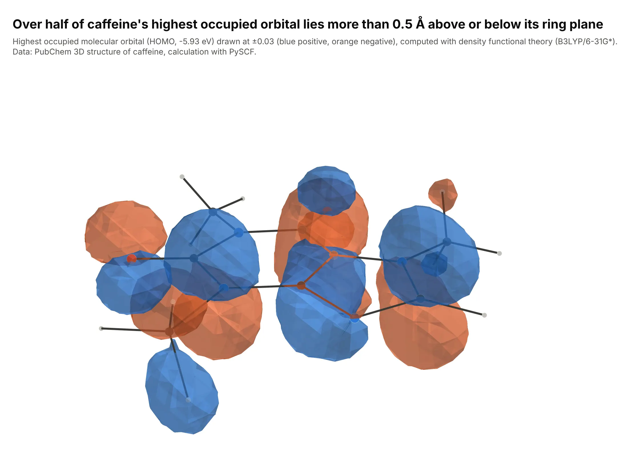
Quantum chemistry. Chemists draw an orbital as two isosurfaces at the same absolute value, one per sign of the wavefunction. More than half of caffeine's highest occupied molecular orbital lies over 0.5 Å from the plane of its rings, which is why the lobes sit above and below it. Data: PubChem 3D structure, calculation with PySCF.

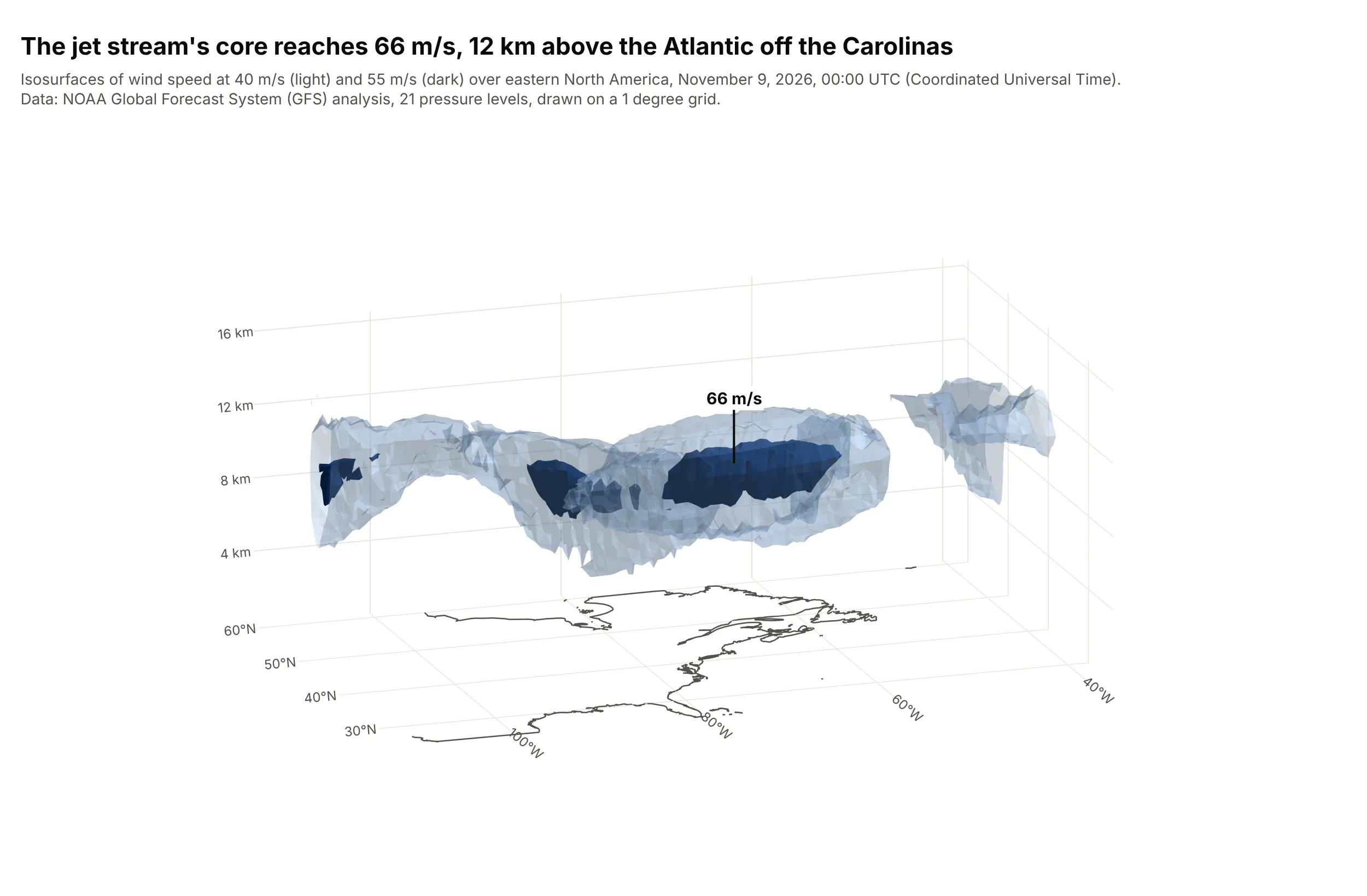
Weather. The jet stream is a tube of fast air, and nested isosurfaces at 40 and 55 meters per second show its outline and its core, which reaches 66 m/s at 12 km, in a model analysis of November 9, 2026. Data: NOAA Global Forecast System (GFS) analysis.

A short history

The standard way to compute an isosurface is marching cubes, published in 1987 by William Lorensen and Harvey Cline to build triangle models of constant-density surfaces from 3D medical scans (ACM SIGGRAPH, doi:10.1145/37402.37422). The algorithm visits every small cube of the grid, checks which corners are above the iso-value, and adds the triangles that separate them. Tools such as MATLAB (isosurface(X,Y,Z,V,isovalue)), the Visualization Toolkit (VTK) and Plotly all produce the same kind of surface. Medical imaging came first, and the engine block above shows the same method on an industrial part.

Alternatives to an isosurface plot

Here's the same ocean temperature cube drawn six ways. Some are better for the question, some worse, some just different:

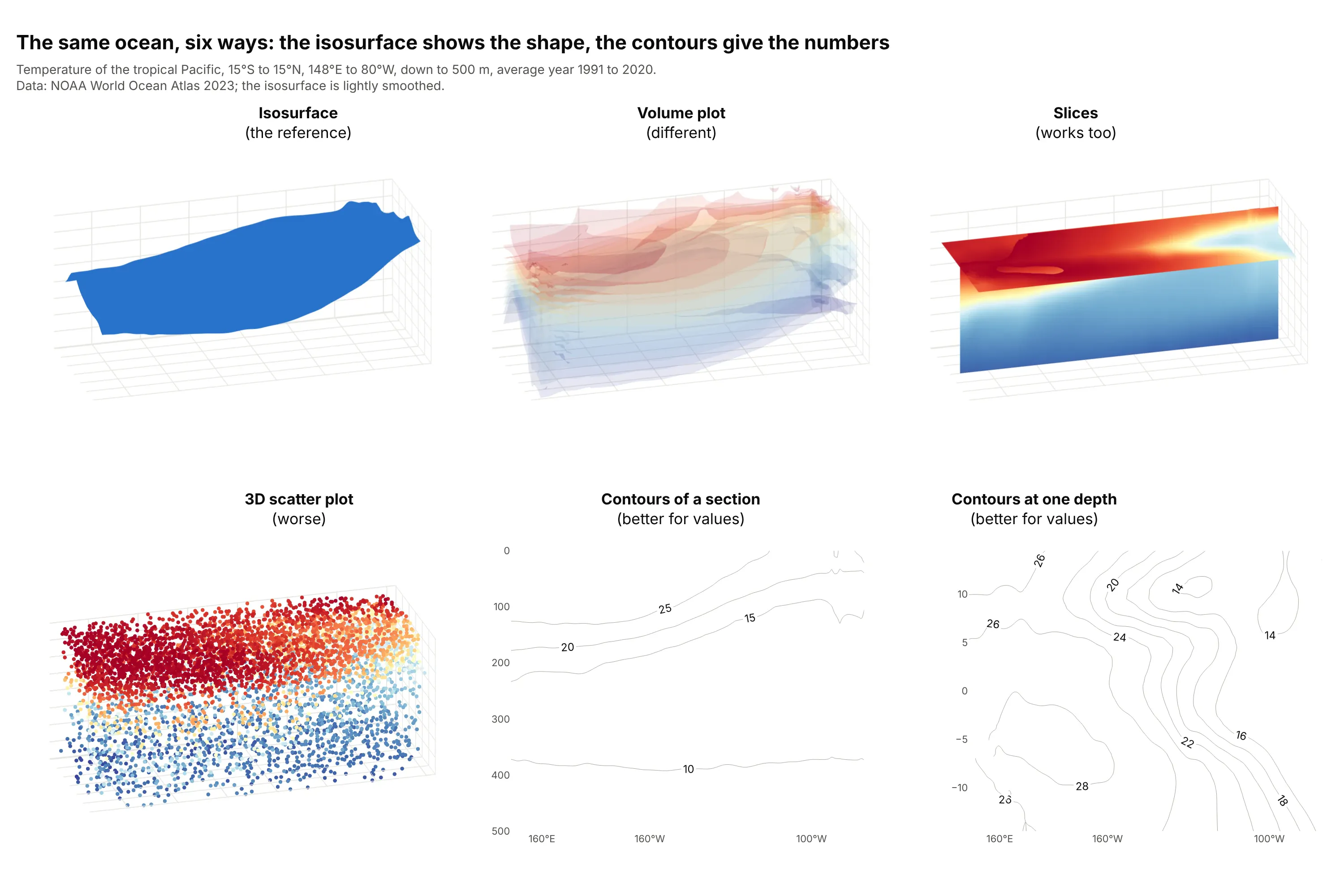
• Isosurface (the reference). One surface at one value, best for the shape of a boundary and the one number it needs.
• Volume plot (different). Many translucent surfaces at once, so the whole range of values shows as a cloud. It reads as a feeling for the structure, and the exact depth of any layer is harder to find.
• Slices (works too). A plane through the cube colored by the actual values. Slices carry every value on the plane and need no iso-value, which suits a field with no single threshold of interest, as in example 6 below.
• 3D scatter plot (worse). Sampled cells as colored dots. Dots hide each other, and sampling leaves holes where the surface should be.
• Contours of a section (better for values). A contour plot of one vertical plane, as in the figure below. It gives the exact depth of every level and needs no 3D camera.
• Contours at one depth (better for values). A map of one level with labeled lines. When the field is a function of two coordinates only, a 3D surface plot fits better than an isosurface, and for a CT or magnetic resonance imaging (MRI) slice an image plot shows the pixels directly.

A contour plot of a section is the slice of an isosurface, which is how the two charts relate. Here is the same 20°C line as a contour on the equator's section and as part of the whole surface:

How to make an isosurface plot

With AI

ChatGPT, Claude Code, GitHub Copilot, Cursor and other AI tools are excellent at writing Plotly code. Name Plotly in the prompt, and say which iso-values to draw and how to label the axes:

With Plotly Studio

Plotly Studio is a desktop app where you point an AI at a dataset and it builds charts and a Dash app around your questions. Ask for an isosurface the same way:

Show the 20°C isosurface of the tropical Pacific from the World Ocean Atlas file as a 3D chart with depth in meters, a slider that moves the iso-value from 10 to 28°C, and a label on the equator's depth at 150°E and 90°W.

Make an isosurface plot in Python or JavaScript

This is the code AI tools write under the hood. In Python, go.Isosurface takes the position of every cell as flat lists and one value per cell, and the Plotly isosurface documentation covers more of the options:

For a volume plot, swap in go.Volume with the same arguments, a range such as isomin=12, isomax=28, surface_count=12 and opacity=0.1. In JavaScript, plotly.js draws both from the same trace types:

You can make a volume plot or slices with the same data: use type: "volume" with opacity and surface.count, or slices: {z: {show: true, locations: [0]}} on an isosurface trace with surface: {show: false}.

Share it

Every Plotly chart has a Share chart button (the cloud icon in its toolbar) that uploads it to Plotly Cloud and gives you a link. Only you can see it until you change its visibility.

For a live app, put the chart in a Dash app and publish it with the Plotly Cloud CLI. Coding agents can run these commands for you:

If your data has to stay in your own cloud or data center, publish to Dash Enterprise instead.

Dos and don'ts

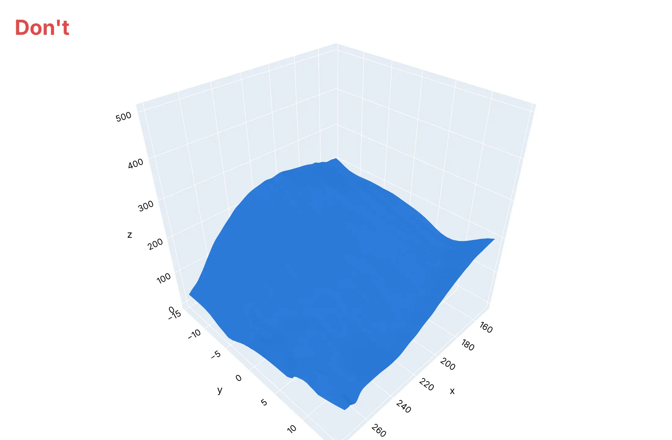
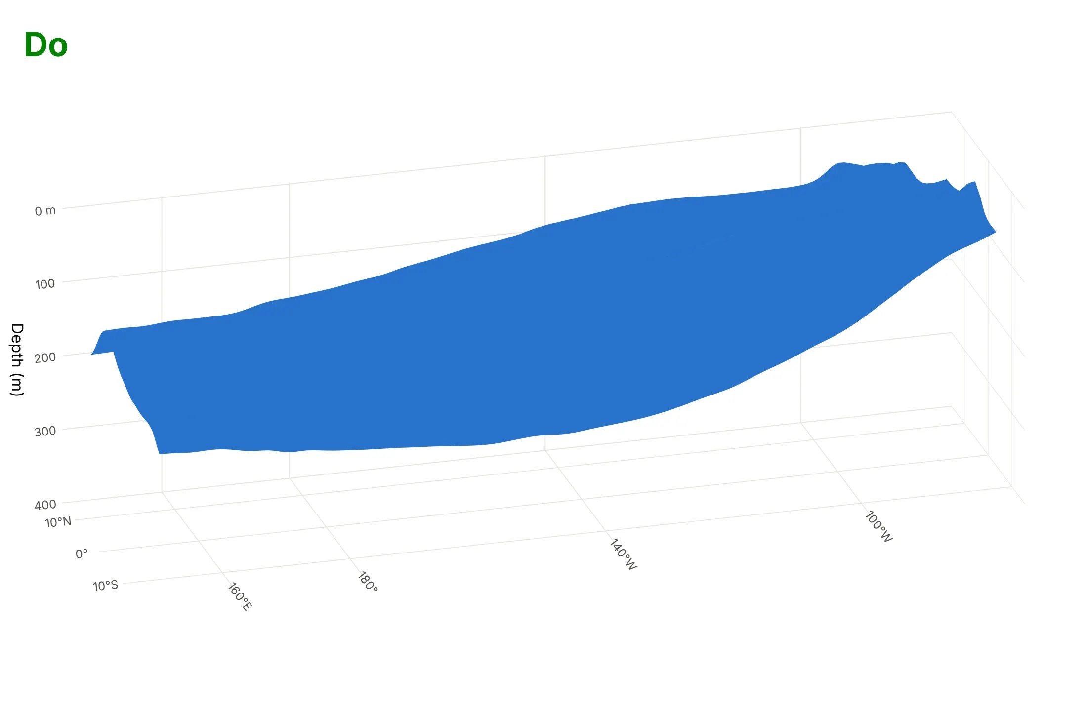
Most of the work in a readable isosurface is the axes: the depth direction, the units and the proportions of the box. Here is the same 20°C surface both ways, in the same blue.

Don't plot depth as a positive number so the sea surface ends up at the bottom, leave the default cube aspect ratio that squeezes 131 degrees of longitude into the same length as 500 m of depth, keep the default axis titles x, y and z with raw decimal ticks, and leave the shaded background panes:

Do plot depth as negative z with ticks in meters, show degrees on the horizontal axes, set the aspect ratio so the layer's tilt is visible, use an orthographic camera and drop the background panes:

Checklist

Do

• Say the iso-value and its unit in the title or subtitle.
• Put depth, height or time in the direction readers expect, and give every axis units.
• Set aspectmode="manual" or "data", and say so when you exaggerate a direction.
• Use a few surfaces with different opacity when you compare levels, and a single opaque one when you show a shape.
• Mark a reference (the equator, a molecule's atoms, a coastline on the floor) so readers can orient themselves.
• Prefer an orthographic camera for measurement and a perspective camera for a feeling of depth.

Don't

• Draw many opaque nested surfaces; the outer ones hide the inner ones.
• Leave isomin and isomax unset unless you want the default surfaces near the extremes of the data.
• Pass NaN cells to go.Isosurface; fill or mask them first.
• Choose an iso-value without checking its effect; example 3 shows how much it can change the result.

Options to customize

A Plotly isosurface is go.Isosurface and a volume plot is go.Volume, and they share most options. The full lists are in the isosurface reference and the volume reference.

1. x, y, z, value: flat arrays with one entry per grid cell; the grid must be complete, with every combination of positions present.
2. isomin, isomax: the range of iso-values to draw; set both to the same number for one surface.
3. surface_count (surface.count): how many surfaces are spread between isomin and isomax.
4. surface_show: turn the surfaces off, to show only caps or slices.
5. surface_fill, surface_pattern: how much of a surface is filled, from 0 to 1, and which parts are drawn.
6. caps: x_show, y_show and z_show draw the faces of the box where the field is in range; turn them off to show only the surface.
7. slices_x, slices_y, slices_z: planes through the cube at given locations, colored by the field.
8. opacity: the opacity of every surface; for a volume plot, one surface adds only a little.
9. opacityscale (go.Volume): a transfer function that sets opacity by value, such as "extremes", "min", "max", "uniform" or your own list.
10. colorscale, cmin, cmax, showscale, colorbar: how values map to color; a two-color scale draws positive and negative lobes in different colors.
11. flatshading, lighting, lightposition: smooth or faceted shading and how the surface catches light.
12. contour: lines drawn where a surface meets the box.
13. scene.aspectmode, scene.aspectratio, scene.camera.projection: the proportions of the box and an orthographic or perspective camera.
14. go.Mesh3d with intensity: draw a surface you computed with marching cubes, colored by another field, as in example 5.

More isosurface and volume plot examples

Six more plots built from real public data, from medicine-adjacent crystallography to oil reservoirs, with the technique that makes each one work and a prompt to rebuild it.

1. A drug inside its electron density

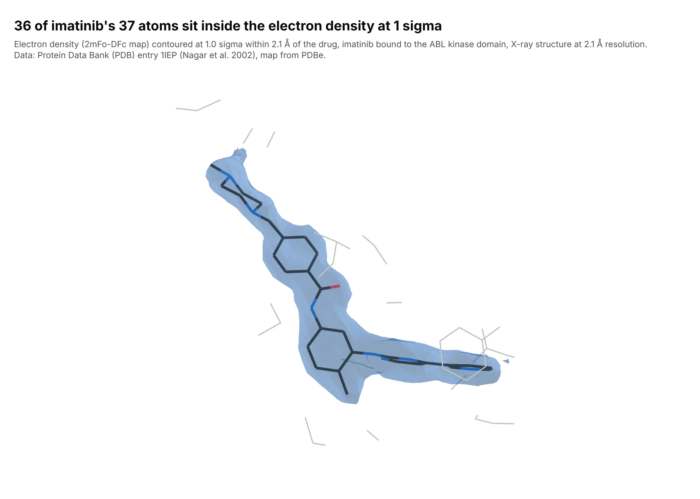
X-ray crystallographers judge a drug's fit by drawing the electron density map at 1 sigma, one root mean square (rms) of the map, and checking that the atoms sit inside the surface. 36 of imatinib's 37 non-hydrogen atoms do, and the 37th sits at 0.99 sigma. Data: Protein Data Bank entry 1IEP (Nagar et al., 2002, Cancer Research 62:4236), map from the Protein Data Bank in Europe (PDBe) at 2.1 Å resolution.

Tip: draw only the density within about 2 Å of the ligand, which crystallographers call carving, so the protein's density doesn't bury it.

2. Rock porosity on the faces of a reservoir model

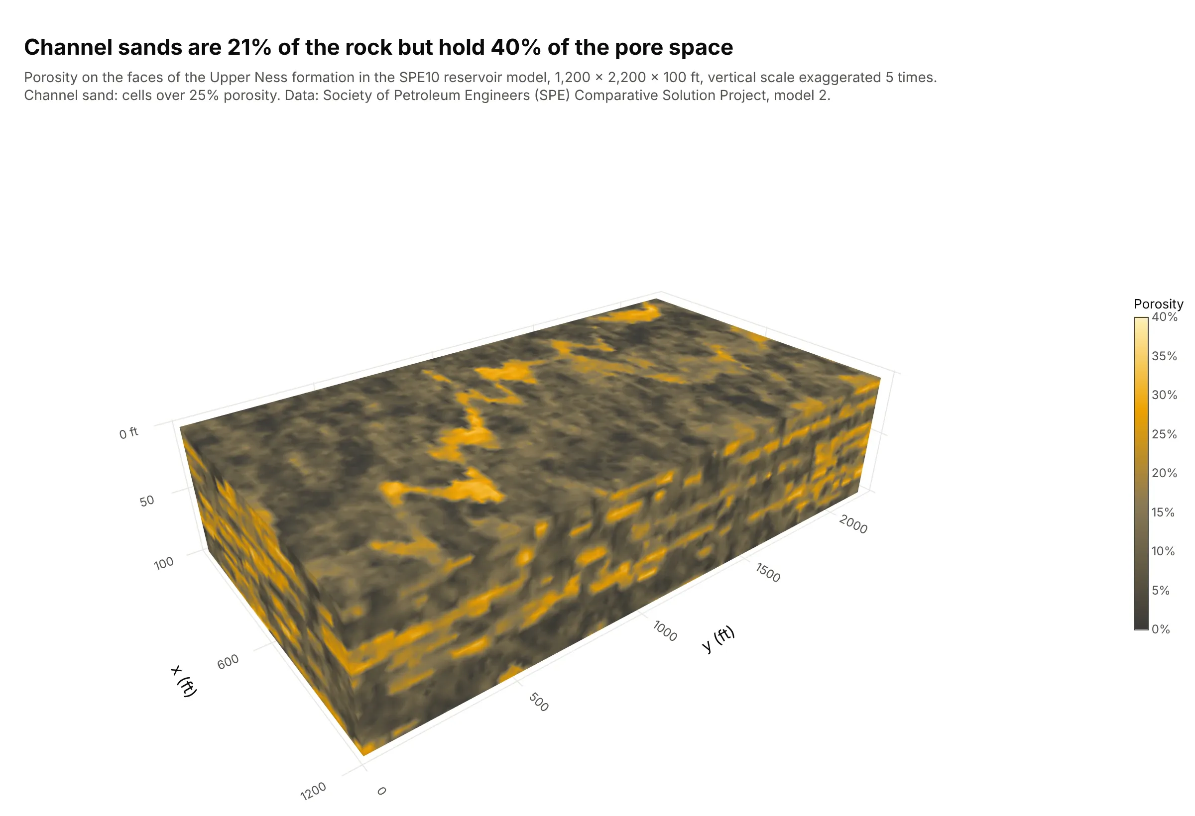
Reservoir engineers inspect a grid property as a colored block. Cells over 25% porosity, the channel sands, are 21% of the Upper Ness formation's rock but hold 40% of its pore space. Data: Society of Petroleum Engineers (SPE) Comparative Solution Project, model 2 (SPE10; Christie and Blunt, 2001).

Tip: surface_show=False with the caps on draws the outside faces of a block colored by value, which is the common way to look at a reservoir grid.

3. How the iso-value changes the connected sand

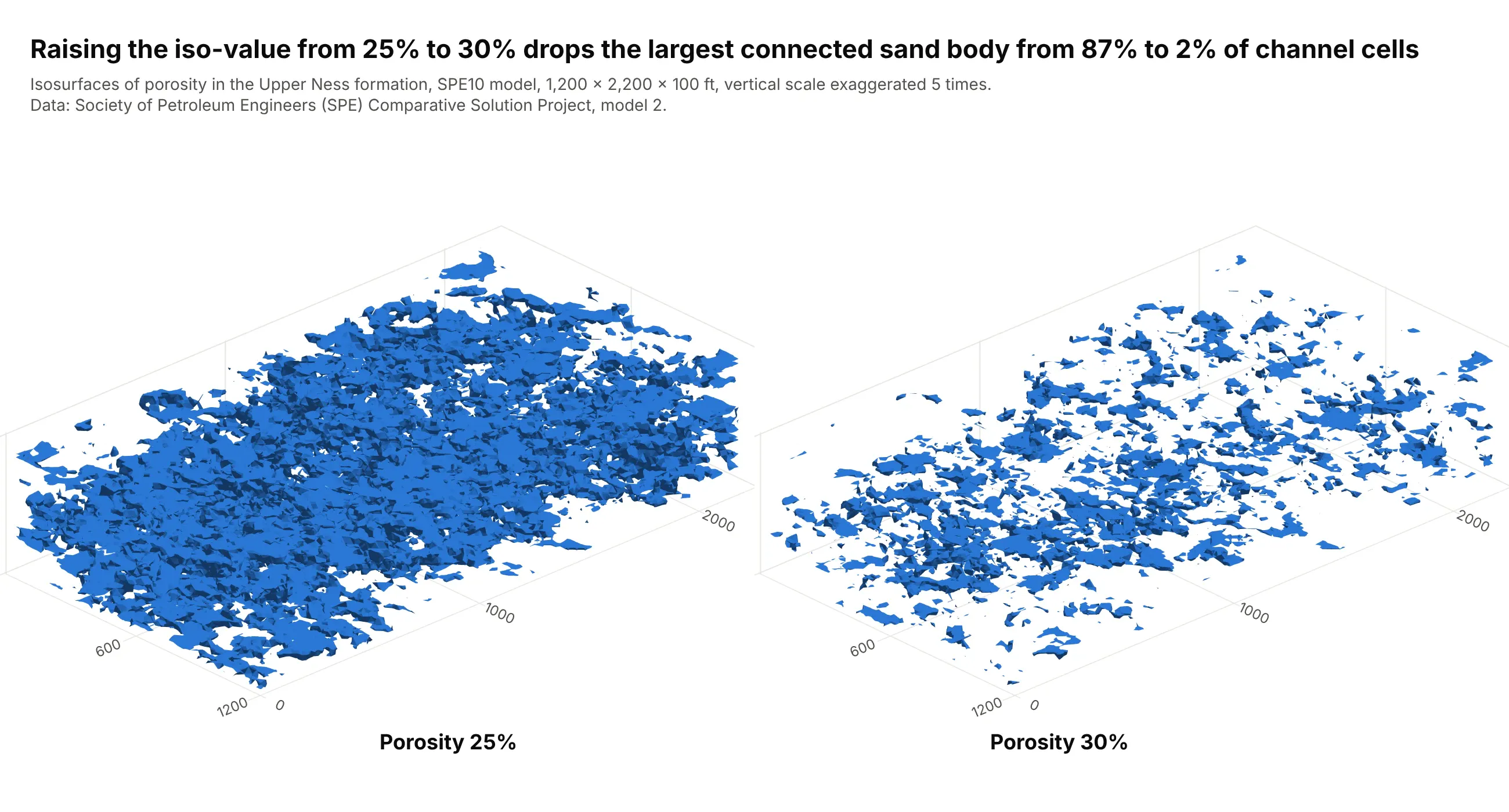
The same model at two iso-values shows why the choice matters: at 25% porosity, 87% of the channel cells belong to one connected body, and at 30% the largest body holds 2%. Oil only flows through connected sand, so the threshold changes the answer. Data: SPE10 model 2, connected bodies counted on the full grid with cells that share a face (scipy.ndimage.label).

Tip: put two iso-values in two scenes with the same camera when a result depends on the threshold.

4. The electron cloud of aspirin

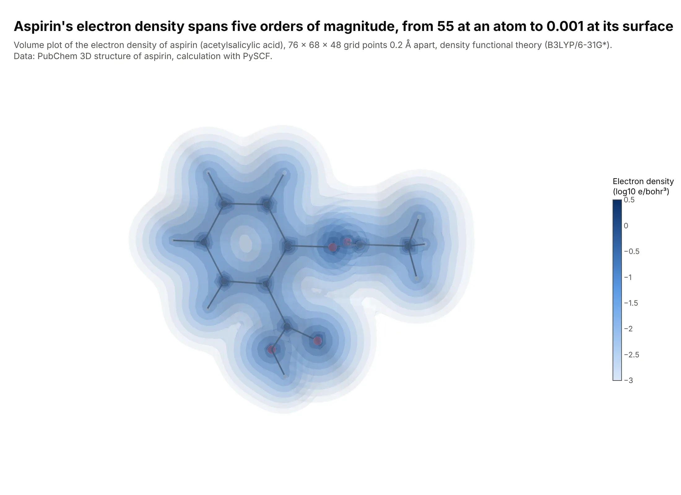
An electron density has no edge, so a volume plot of ten translucent shells shows it better than one surface. The density falls from 55 electrons per cubic bohr at an atom to 0.001, the value chemists use to define a molecule's surface. Data: computed with density functional theory (B3LYP/6-31G*) in PySCF at the PubChem 3D structure of aspirin.

Tip: plot the logarithm of a field that spans orders of magnitude, so the shells are spread evenly.

5. Coloring a surface by another field

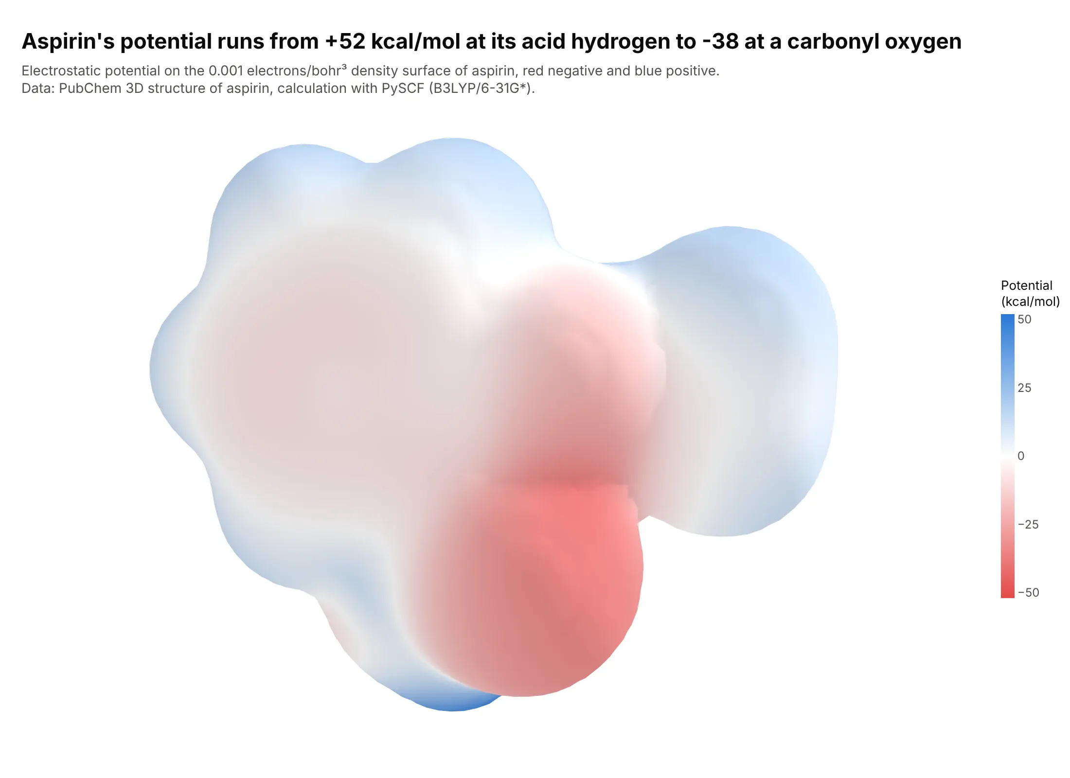
An isosurface is colored by the field that defines it, so to color it by a second field you compute the surface once and draw it as go.Mesh3d with intensity. Here the surface is the density at 0.001, and the color is the electrostatic potential, from +52 kcal/mol at aspirin's acid hydrogen to -38 at a carbonyl oxygen. Data: computed with PySCF (B3LYP/6-31G*) at the PubChem 3D structure of aspirin.

Tip: center a diverging scale on zero with cmin and cmax of the same size, and follow the chemists' habit of red for negative.

6. Slices through the salinity of the North Atlantic

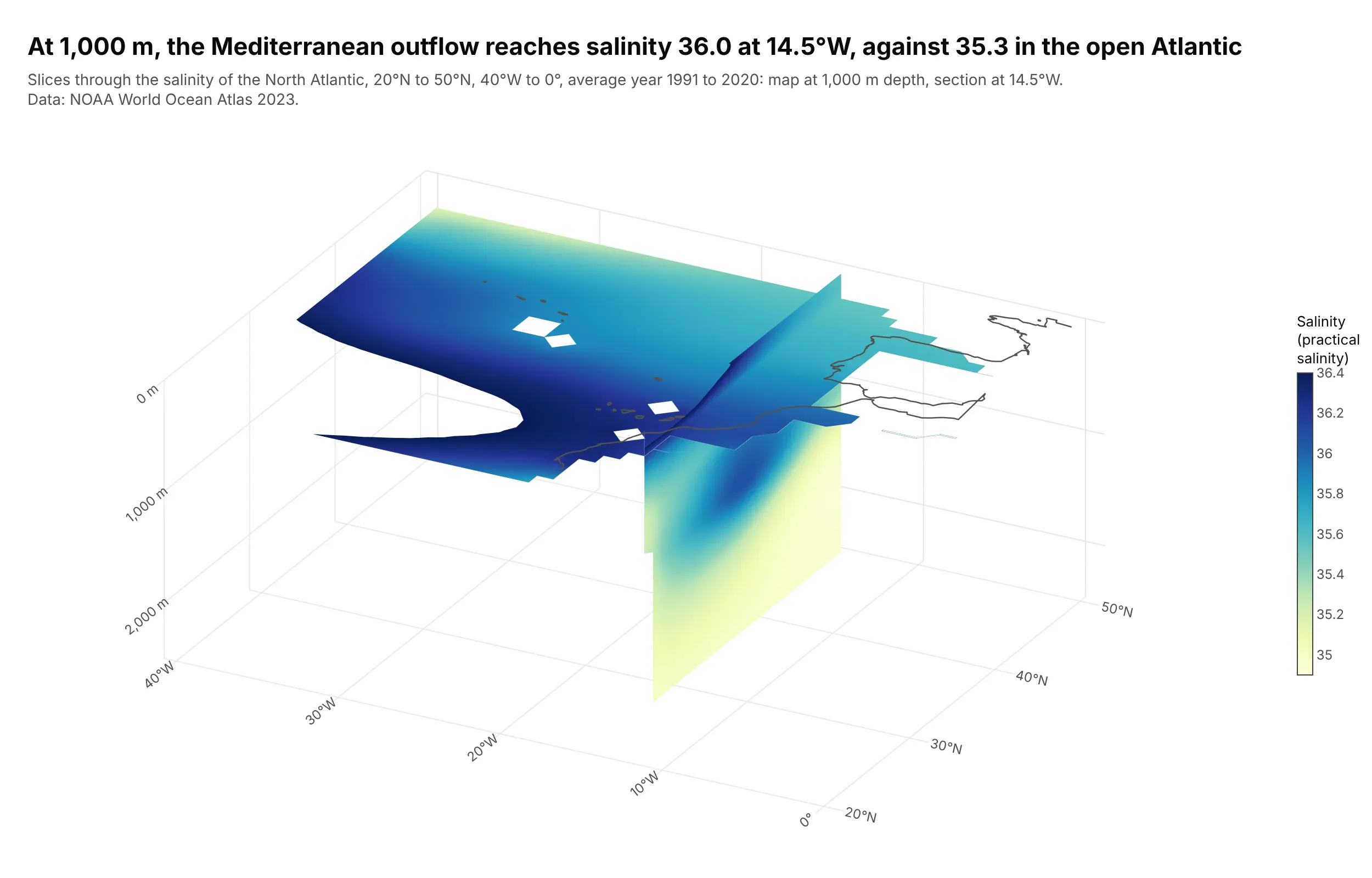
Slices carry every value on the plane, so they suit a field with no single threshold of interest. The salty water that leaves the Mediterranean spreads west at about 1,000 m, reaching a salinity of 36.0 at 14.5°W against 35.3 in the open Atlantic at the same depth. Data: NOAA World Ocean Atlas 2023, annual mean salinity, 1991 to 2020.

Tip: set the color limits isomin and isomax to the range you care about, and set land cells to a value outside it so they are cut out of the slice.