2D Histograms and Density Contour Plots - A Complete Guide

TL;DR

• A 2D histogram splits the plane of two numeric variables into a grid of cells and colors each cell by how many points fall in it, so hundreds of thousands of overlapping points become a readable picture of where the data is dense. A 2D histogram contour plot (density contour) draws the same counts as lines or bands of equal count.
• 2D histograms are also known as density heatmaps and bivariate histograms, and with a histogram of each variable in the margins as joint plots; the contour version is also called a density contour plot. They are similar to marginal plots, hexbin plots, 2D density plots, heatmaps, and contour plots.
• The setting that changes what you see is the cell size: too small and the chart turns into noise, too big and the groups melt together. Pick it yourself, and use a log color scale when the busiest cells hold thousands of times more points than the rest.
• In Python, px.density_heatmap and px.density_contour make one in one line of code (the histogram2d and histogram2dcontour traces), with marginal_x and marginal_y for histograms in the margins. Plotly drew 10 million points as a 2D histogram in 2.6 seconds in our test.

What is a 2D histogram?

2D histograms look like this:

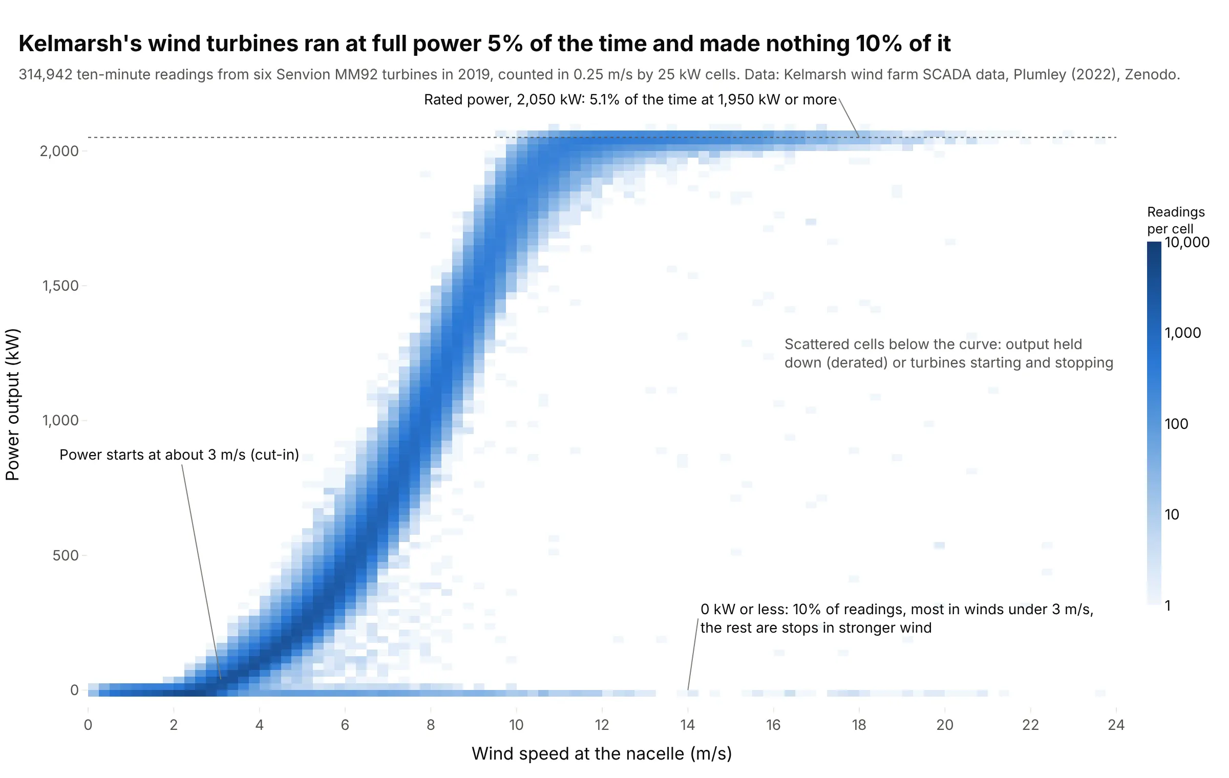
Data: Kelmarsh wind farm SCADA data 2019, Plumley (2022), Zenodo, CC BY 4.0.

How do you read a 2D histogram? In the example above, notice these things:

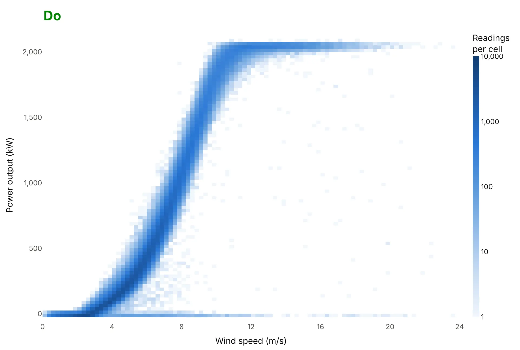
• Each small rectangle is a cell 0.25 m/s wide and 25 kW tall, and its color is how many of the 314,942 ten-minute readings fell in it. Each reading is a 10-minute average logged by the turbine’s supervisory control and data acquisition (SCADA) system.
• The color scale is logarithmic: each step on the color bar is 10 times more readings. The dark S is the turbines’ power curve, where most readings sit, and the pale cells around it hold one to a few readings each.
• Power starts at about 3 m/s and reaches the rated 2,050 kW near 11 m/s. The flat band at the top shows the turbines at full power, 5.1% of the time.
• The row along 0 kW holds 10% of the readings. Most of them are calm periods under 3 m/s, and the rest are stops in stronger wind, which a scatter plot of 300,000 dots would hide under the curve.

It’s often used for charts like these:

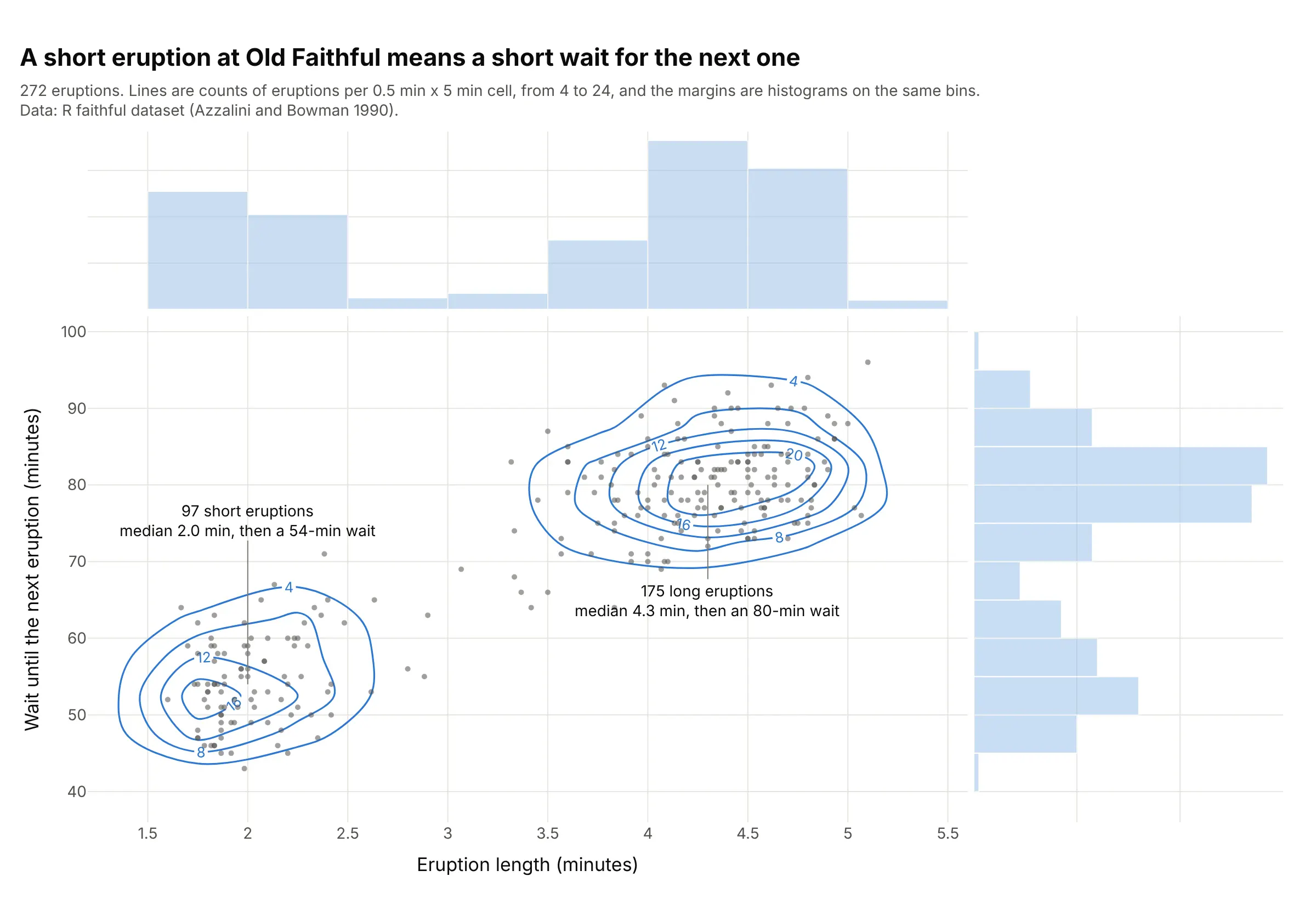
The classic: two groups in two variables. Old Faithful’s 97 short eruptions are followed by a median wait of 54 minutes and its 175 long ones by 80 minutes, so the length of one eruption predicts the wait for the next. Data: R dataset faithful, Azzalini and Bowman (1990).

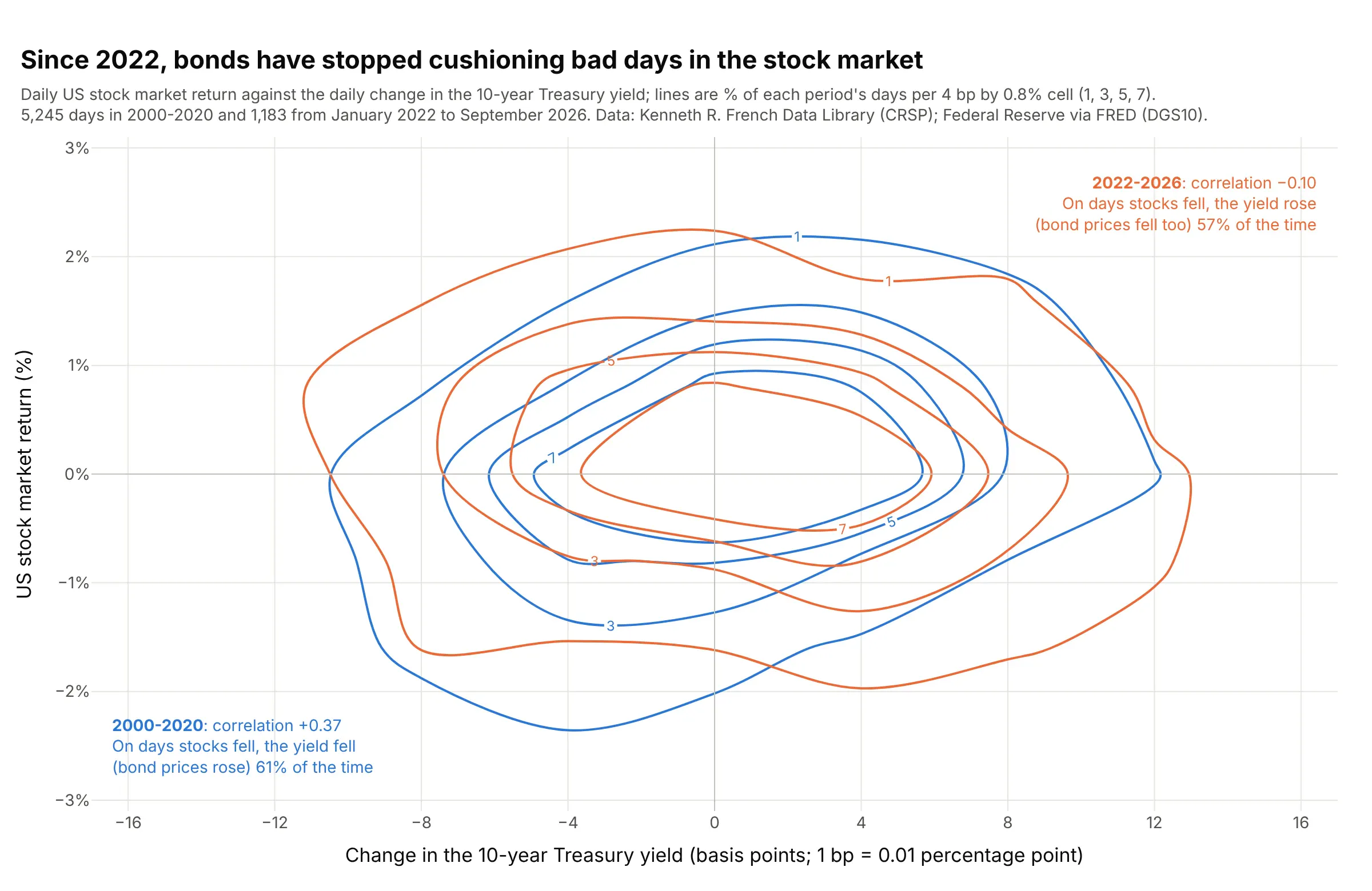
The joint distribution of two returns. From 2000 to 2020, the 10-year Treasury yield fell (so bond prices rose) on 61% of the days the stock market fell; since 2022 it rose on 57% of them, so bonds fell along with stocks. Data: Kenneth R. French Data Library (the Center for Research in Security Prices (CRSP) market return) and Federal Reserve Economic Data (FRED, series DGS10).

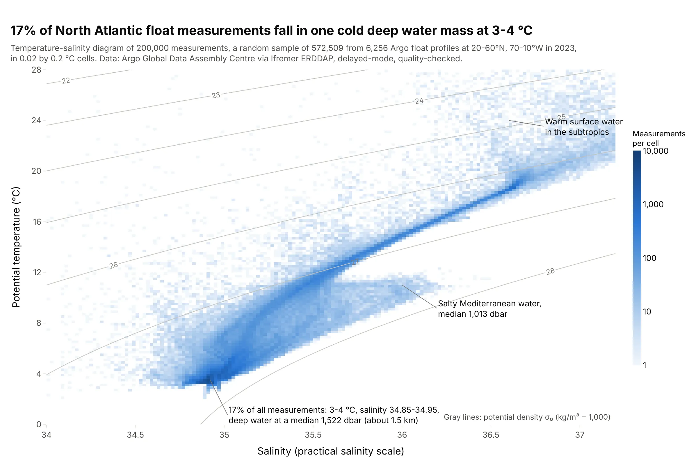
Temperature-salinity (T-S) diagrams in oceanography. Oceanographers recognize water masses as dense clusters on a T-S diagram: 17% of these North Atlantic measurements fall at 3-4 °C and a salinity of 34.85-34.95, at a median depth of about 1.5 km, and salty Mediterranean water shows up as a tongue near 1,000 m. Data: Argo floats via Ifremer’s data server, 2023.

How a 2D histogram counts points

A one-dimensional histogram splits one axis into bins and counts the values in each. A 2D histogram does the same on two axes at once, so the bins become a grid of rectangles, and a contour plot of it joins places with equal counts.

Step 1: draw a grid and count. Here are Old Faithful’s 272 eruptions in cells 0.5 minutes wide and 5 minutes tall. The busiest cells hold 23 and 24 eruptions, and most of the grid is empty:

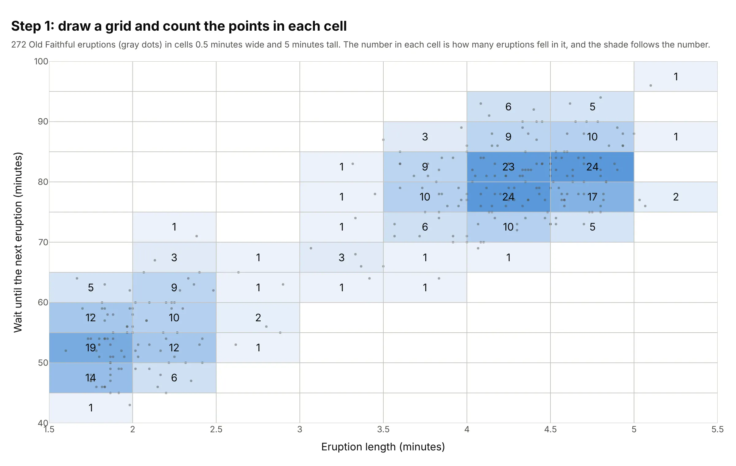
Step 2: draw lines through equal counts. A 2D histogram contour plot takes the same counts, treats each as a height at the middle of its cell, and draws contour lines through the places where the count would be 4, 8, 12, and so on, filling the bands between them. The contour levels are counts per cell, so the labels change if you change the cell size:

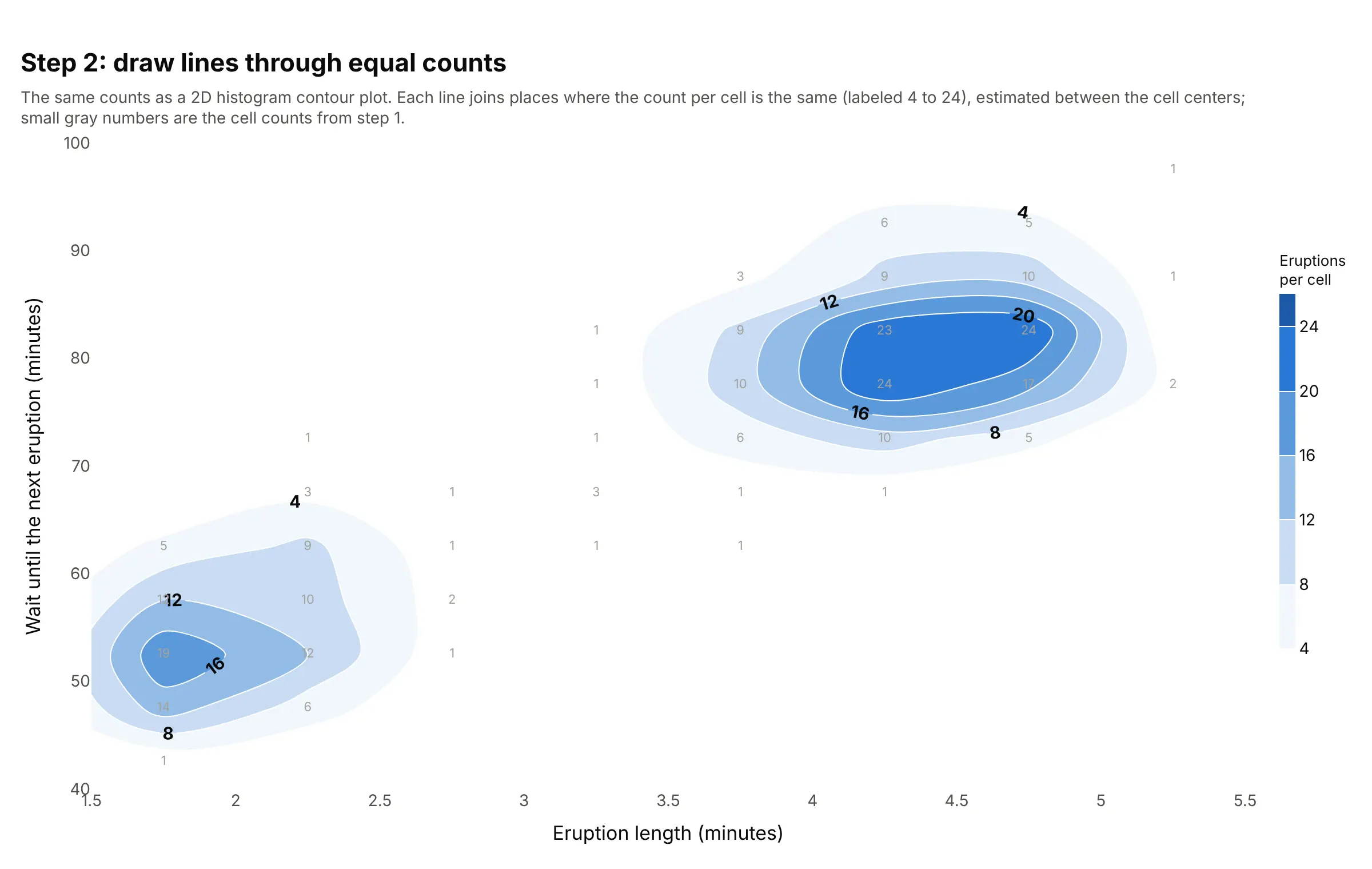
The lines are smooth only because they are interpolated between cell centers; the information is still the counts of step 1. That’s the main difference from a 2D kernel density estimate (KDE), which puts a small smooth bump on every point and adds them up, so its contours don’t depend on a grid at all.

Choosing the cell size

The cell size plays the part that the bin width plays in a histogram. With cells that are too small, each cell holds zero or one point and the chart is noise. With cells that are too big, the shape of each group disappears into a few blocks:

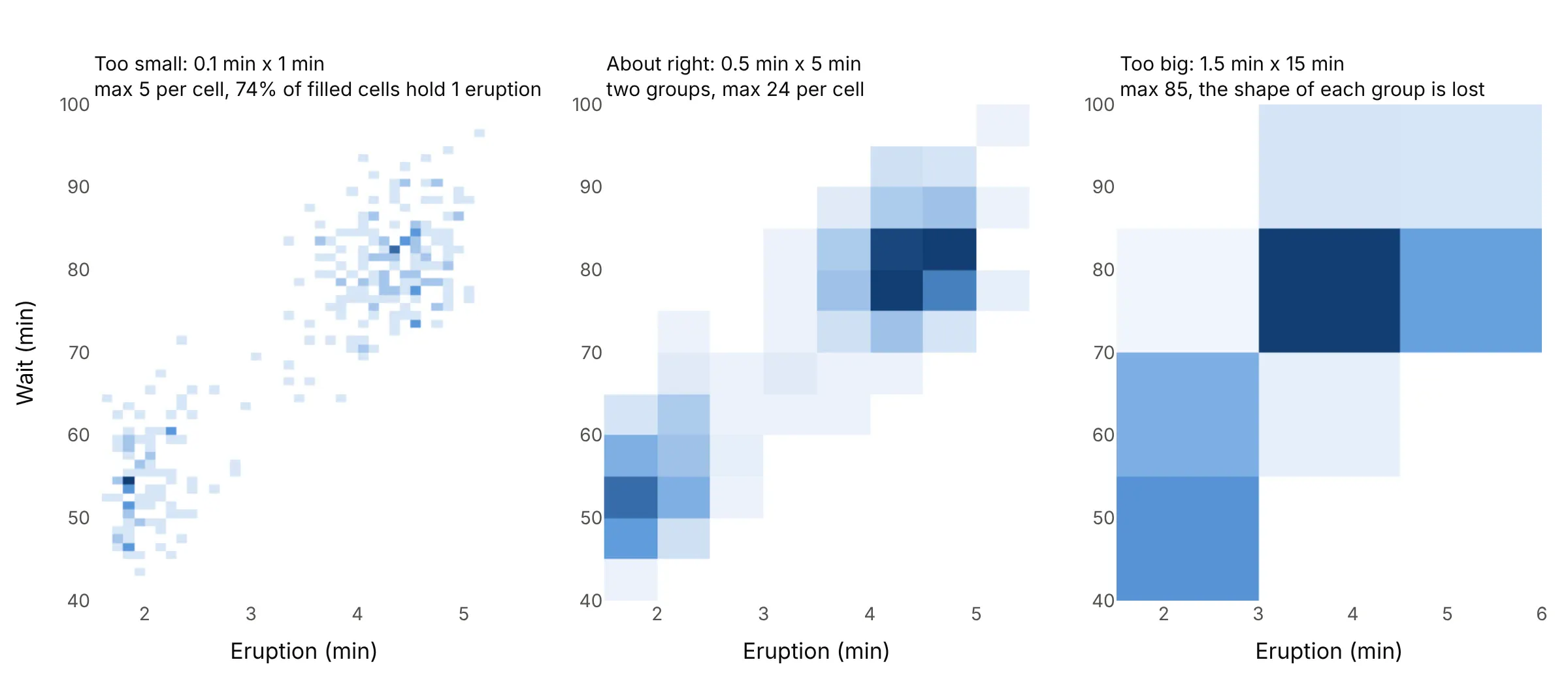
A few rules help:

• Aim for the busiest cells to hold at least 10 to 20 points; with 272 points, that means a grid of about eight by 12 cells, not 40 by 60.
• MATLAB’s histogram2 offers Scott’s rule, a cell width of 3.5 × standard deviation × n^(−1/4) on each axis. For Old Faithful it gives 0.98 by 11.7 minutes, which is too coarse for data with two groups, so treat it as a starting point and try half of it.
• Use round numbers that match the data’s resolution: 0.25 m/s for wind speed, 1 mmHg for blood pressure, and 1 second for a wave period. If the data are rounded, like Old Faithful’s waits in whole minutes, make the cell a multiple of the rounding or some cells will get more values than others.
• With hundreds of thousands of points, you can afford small cells; then use a log color scale so the sparse cells still show.

A short history

Francis Galton made one of the first 2D histograms in 1886, a table of 928 adult children’s heights against their mid-parent’s height in one-inch classes, in “Regression towards mediocrity in hereditary stature”. He smoothed it by writing at each corner “the sum of the entries in the four adjacent squares”, and noticed that “lines drawn through entries of the same value formed a series of concentric and similar ellipses”, which led him to the idea of regression (Friendly and Denis 2005 trace the story). This is his table redrawn with Plotly, with contours through the same four-cell sums:

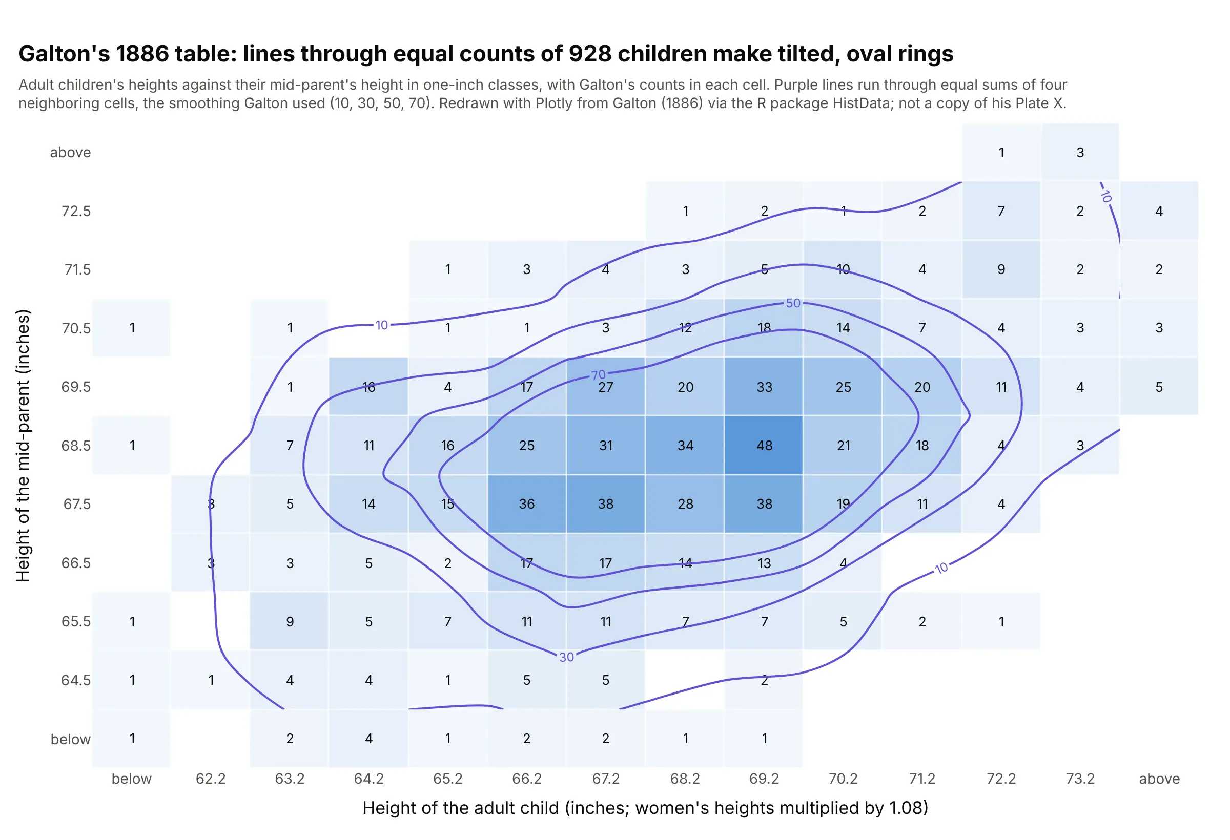
Data: Galton (1886), Table I, via the R package HistData (Galton). A redraw from his data, not a copy of his Plate X.

Hexagonal bins followed a century later, when Daniel Carr and colleagues proposed them for scatter plots with too many points (Carr et al. 1987).

Alternatives to a 2D histogram

Here’s the same set of 314,942 turbine readings drawn six ways. Some are better for the question, some worse, some just different:

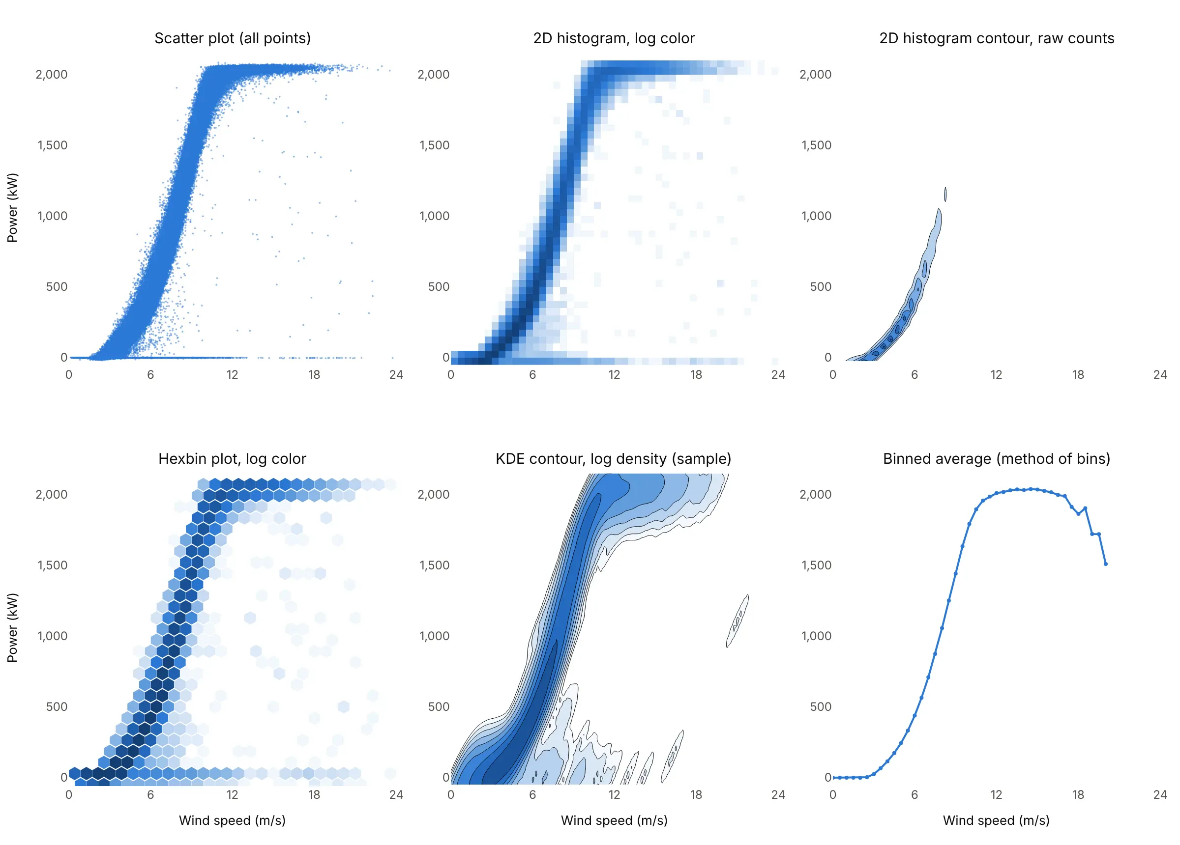
• Scatter plot (worse above about 10,000 points, better below). It shows every point, including the rare ones, but here the curve is a solid band and you can’t tell 10 readings from 10,000.
• 2D histogram contour of the raw counts (worse here, better for data within one order of magnitude). The busiest cells hold over 5,000 readings, so linear contour levels only show the low-wind end of the curve. It works well when the counts are similar in size, as in the Old Faithful and stock market examples.
• Hexbin plot (works too). Hexagons count the same points with less visible grid structure, and every neighboring cell is the same distance away. With Plotly you draw the hexagons from your own bins, while a 2D histogram is one trace.
• 2D density plot, a KDE contour (works too, for smooth shapes). It needs no grid and gives smooth contours, but evaluating it took seconds on a 20,000-point sample, and it blurs the sharp edge at rated power and the row at 0 kW.
• Binned average line (better for the question “what does the turbine produce at each wind speed”). This is the method of bins that power curve tests use. It summarizes each column in one number, but the average hides the spread, and above 17 m/s a few stops pull it down to 1,510 kW at 20 m/s.
• Heatmap of a matrix (different). A heatmap colors cells by a value you already have, such as a correlation matrix or prices by hour and day. A 2D histogram computes its value by counting points; once counted, you can draw it with go.Heatmap, as several examples here do. A contour plot is the same relationship for contours: go.Contour draws a grid you give it, go.Histogram2dContour makes the grid from points.

How to make a 2D histogram

With AI

ChatGPT, Claude Code, GitHub Copilot, Cursor, and other AI tools are excellent at writing Plotly code. Name Plotly in the prompt, and say what the cells should be and how to color the counts:

With Plotly Studio

Plotly Studio is a desktop app where you point an AI at a dataset and it builds charts and a Dash app around your questions. Ask for a 2D histogram the same way:

Show a 2D histogram of wind speed against power output for each turbine, with a log color scale, a slider for the cell size, and a dropdown to pick the turbine.

Make a 2D histogram in Python or JavaScript

This is the code AI tools write under the hood. In Python, Plotly Express makes a 2D histogram with px.density_heatmap and a 2D histogram contour plot with px.density_contour, and both take marginal_x and marginal_y for histograms in the margins (marginal plots):

Set xbins and ybins yourself rather than nbinsx and nbinsy, which Plotly treats as a maximum and rounds to nice sizes. Start the contour’s bins one cell before the data and end one after, so the lines close around the groups instead of stopping at the edge.

For hundreds of thousands of points, or for a log color scale, count the cells with NumPy and draw only the counts. The browser then gets 8,544 cells instead of 314,942 points:

In JavaScript, plotly.js bins the points itself with a histogram2dcontour (or histogram2d) trace:

Share it

Every Plotly chart has a Share chart button (the cloud icon in its toolbar) that uploads it to Plotly Cloud and gives you a link. Only you can see it until you change its visibility.

For a live app, put the chart in a Dash app and publish it with the Plotly Cloud command-line interface (CLI). Coding agents can run these commands for you:

If your data has to stay in your own cloud or data center, publish to Dash Enterprise instead.

Dos and don’ts

Most of what makes a 2D histogram readable is the cell size, the color scale, and the labels. Here are the turbine readings both ways, with the same blue color scale.

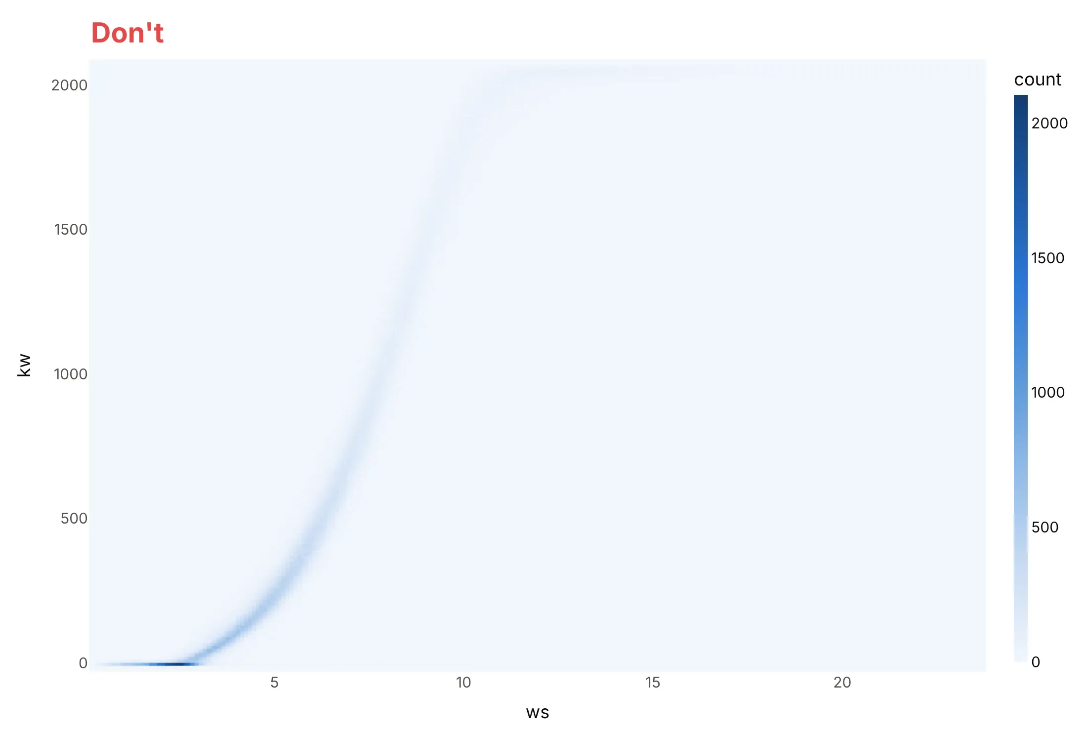
Don’t let a few hundred tiny cells and a linear color scale decide the chart. The busiest cells, idle turbines in calm wind, hold thousands of readings, so everything else fades to the palest blue, and the raw column names ws and kw leave the reader guessing at units:

Do pick cells that match the data’s resolution, color the counts on a log scale with empty cells left white, and write axis and color bar titles in words with units:

Checklist

Do

• Set the cell size yourself (xbins, ybins or np.histogram2d edges) and say it in the subtitle.
• Use a log color scale when counts span more than about two orders of magnitude, and label the color bar in real counts (1, 10, 100).
• Leave empty cells white (NaN), so “no data” doesn’t look like “a little data”.
• Use histnorm="percent" or "probability" when you compare groups of different sizes, as in the stock market example.
• Draw the points under density contours when there are fewer than a few thousand, so readers see how few points the outer lines rest on.
• Add marginal histograms when each variable’s own distribution matters (see the marginal plot guide).

Don’t

• Compare colors between two charts with different cell sizes; the counts per cell change with the area of the cell.
• Use histfunc="avg" on go.Histogram2d without checking the empty cells: they are drawn as an average of 0. Compute averages with pandas and draw them with go.Heatmap (example 3 below).
• Read structure into cells that hold one or two points.
• Use a rainbow color scale for counts; a single-hue scale from light to dark reads as more and less.

Options to customize

A 2D histogram in Plotly is a histogram2d trace (px.density_heatmap) and the contour version a histogram2dcontour trace (px.density_contour). These are the options that matter most; the full lists are in the histogram2d reference and the histogram2dcontour reference.

1. xbins, ybins (start, end, size): the cell edges. Set them yourself; use the same bins for every trace you compare.
2. nbinsx, nbinsy: a maximum number of bins that Plotly rounds to nice sizes. Fine for a first look.
3. histfunc ("count", "sum", "avg", "min", "max") with z: aggregate a third variable per cell instead of counting points.
4. histnorm ("percent", "probability", "density", "probability density"): normalize counts, to compare groups of different sizes or cells of different areas.
5. marginal_x, marginal_y in Plotly Express ("histogram", "box", "violin", "rug"): a distribution of each variable in the margins, the joint plot layout.
6. contours (start, end, size, coloring="fill", "lines" or "heatmap", showlabels, labelfont): the contour levels, which are counts per cell, and how they are drawn.
7. ncontours with autocontour=True: a maximum number of levels when you don’t set them.
8. colorscale, zmin, zmax, reversescale: the color mapping; set zmax when comparing charts.
9. texttemplate="%{z}": print the count in each cell, as in a scatter diagram table.
10. xgap, ygap on go.Heatmap: thin white lines between cells, useful when the cells are few and large.
11. coloraxis: one shared color scale for several 2D histograms in subplots.
12. numpy.histogram2d plus go.Heatmap or go.Contour: bin in Python for log color scales, millions of points, or masks on sparse cells.

More 2D histogram examples

Six more 2D histograms and density contour plots built from real public data, each with its source, the technique that makes it work, and a prompt to rebuild it.

1. Blood pressure categories in US adults

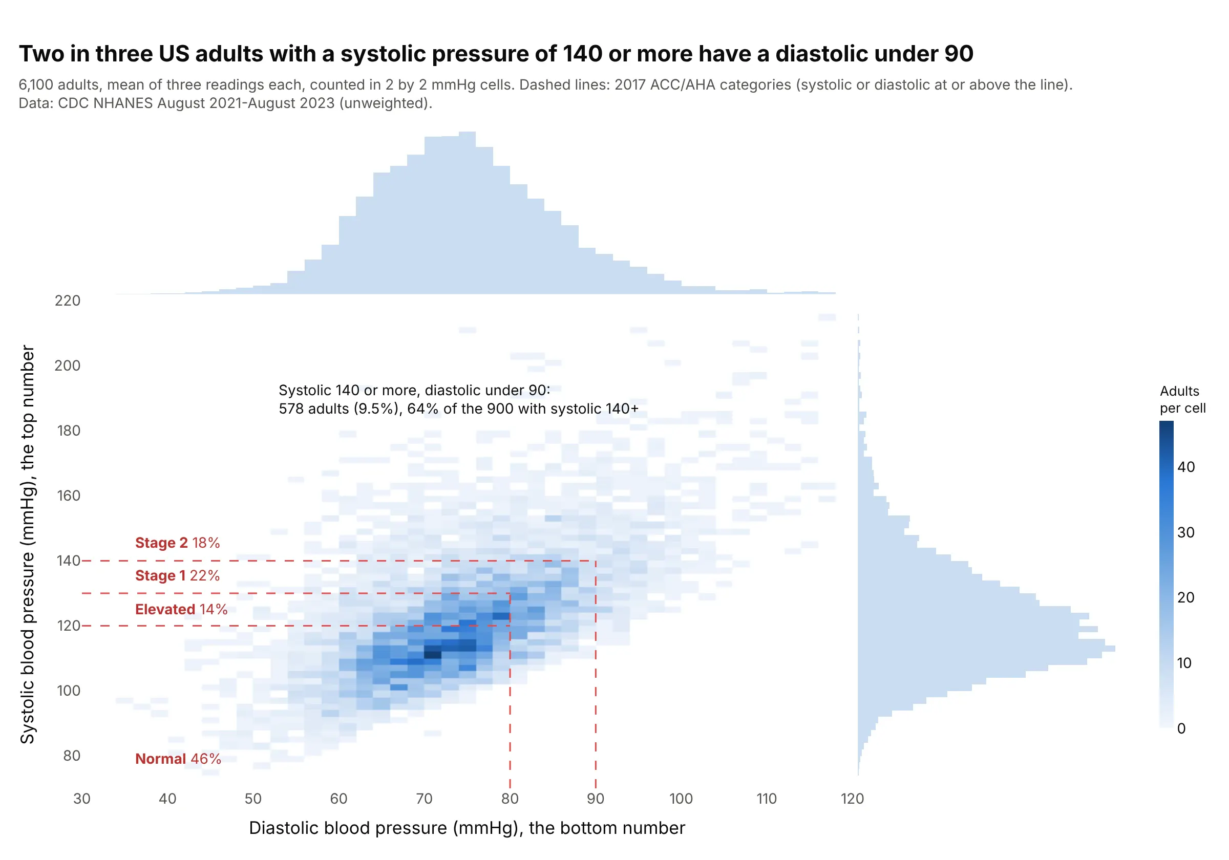
Blood pressure categories are regions of this plane, so the cells show who falls where: 18% of 6,100 adults are in stage 2 hypertension, and of the 900 with a systolic reading of 140 or more, 64% have a diastolic under 90. Data: US Centers for Disease Control and Prevention (CDC), National Health and Nutrition Examination Survey (NHANES) August 2021-August 2023; categories from the 2017 American College of Cardiology and American Heart Association (ACC/AHA) guideline.

Tip: draw guideline thresholds as L-shaped lines, because a category defined by “either number at or above” is a corner, not a box.

2. German power prices by hour of day

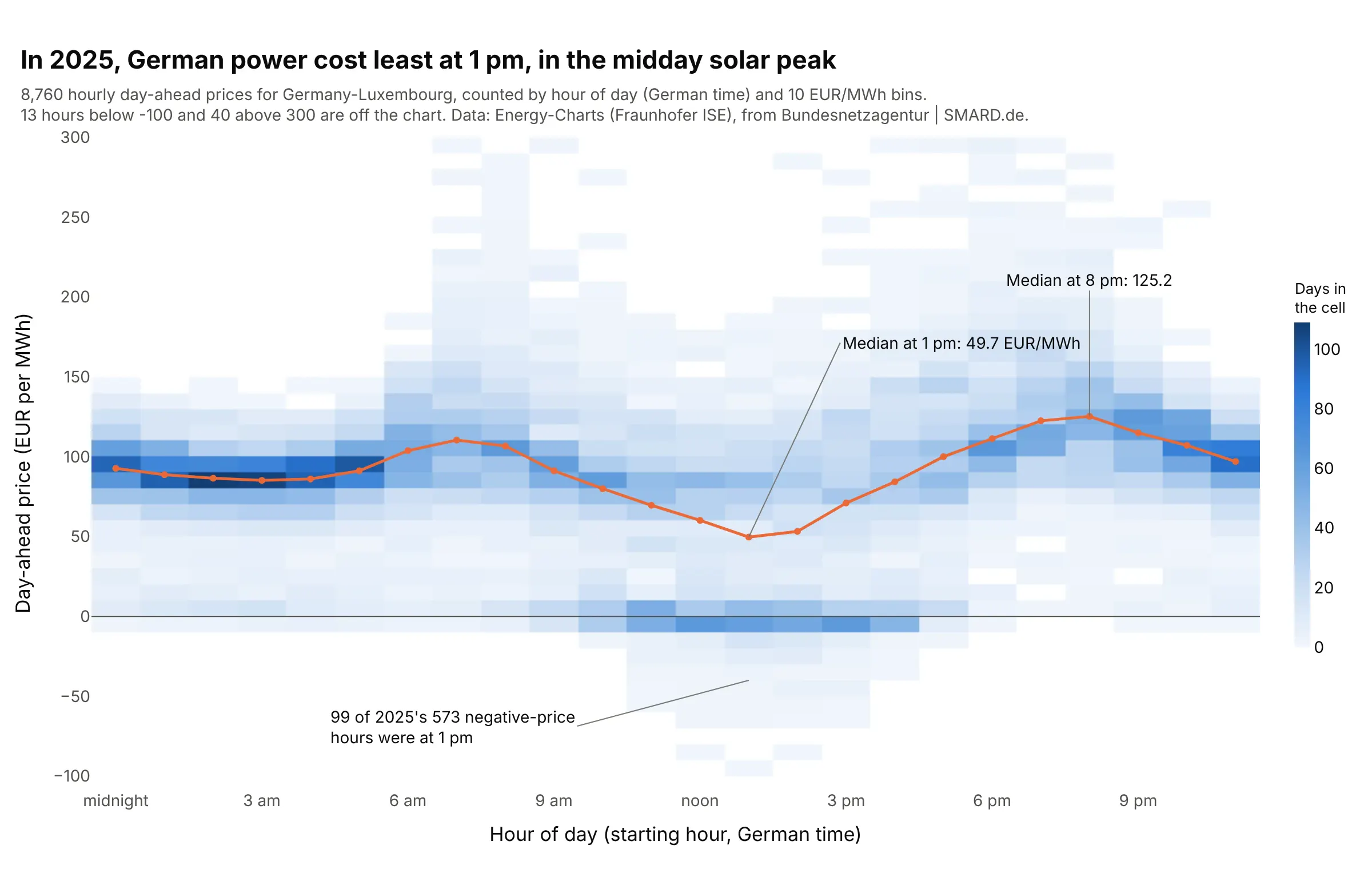
With the hour on the x axis, each column is a year of prices for that hour. The median fell to 49.7 EUR/MWh at 1 pm, in the midday solar peak, and 99 of 2025’s 573 negative-price hours were at 1 pm. Data: Energy-Charts (Fraunhofer ISE), prices from Bundesnetzagentur | SMARD.de.

Tip: when one axis is time of day, every column has the same number of points (365 here), so the counts compare directly without normalizing.

3. Power prices against wind and solar output and demand

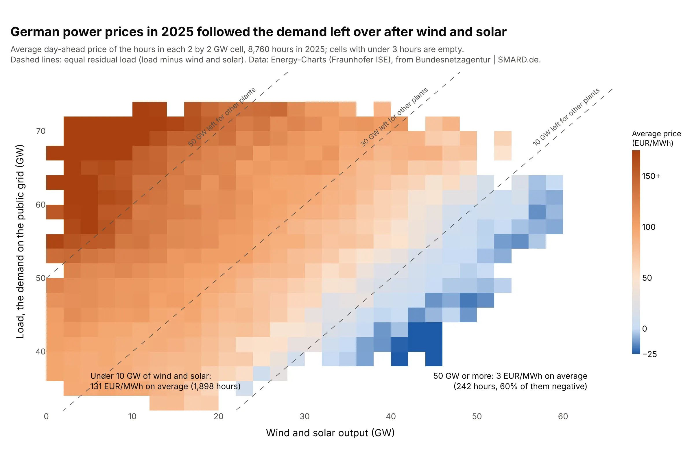
Instead of counting hours, each cell shows their average price. Hours with under 10 GW of wind and solar averaged 131 EUR/MWh and hours with 50 GW or more averaged 3, and the colors follow the diagonals of equal residual load, the demand left for other plants. Data: Energy-Charts (Fraunhofer ISE), 8,760 hours in 2025.

Tip: compute averages with pandas and draw them with go.Heatmap, leaving cells with under three hours empty, because histfunc="avg" paints empty cells as 0.

4. Where home runs come from

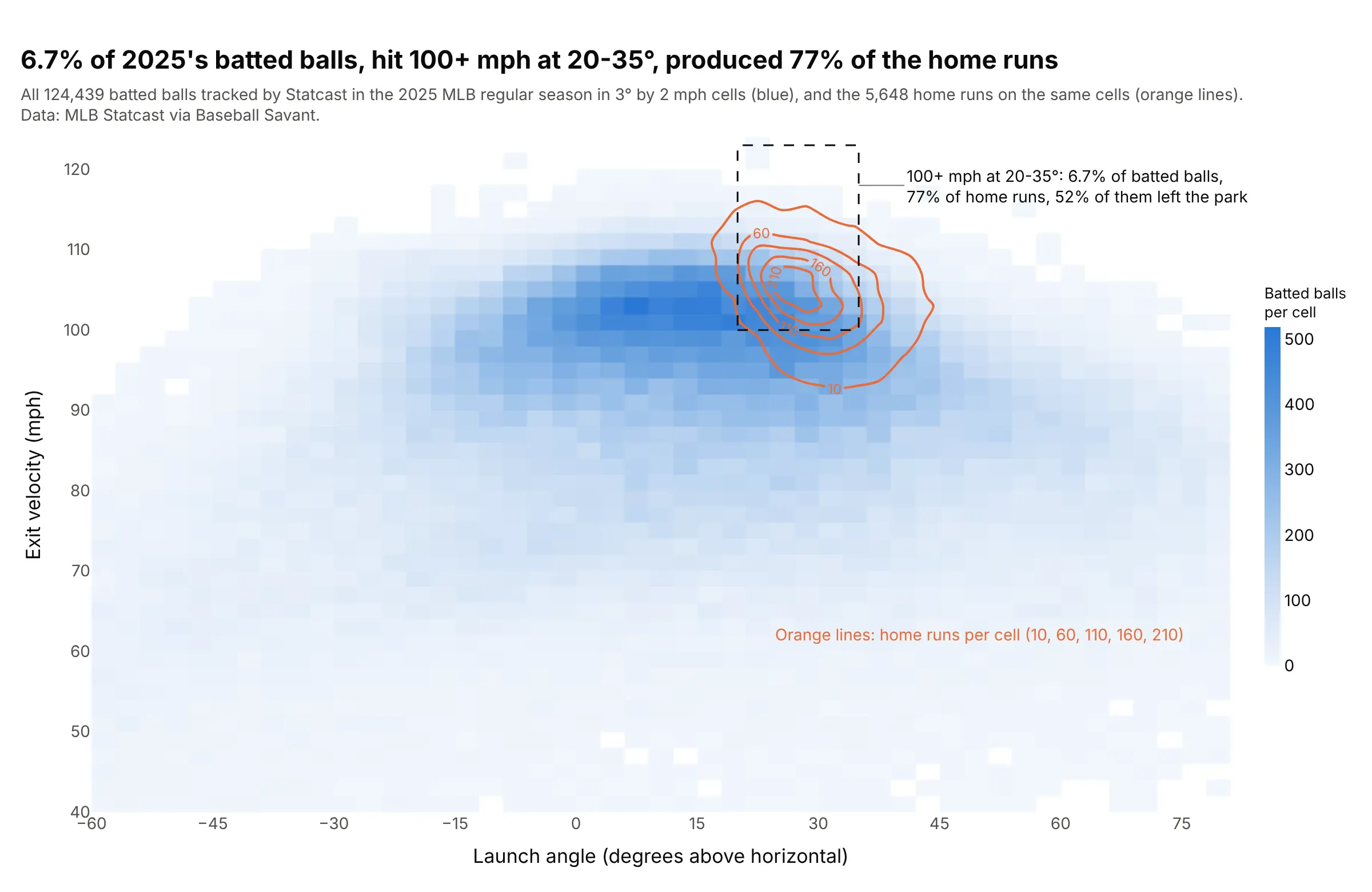
The blue cells are every batted ball tracked in the 2025 Major League Baseball (MLB) regular season, and the orange lines are the home runs alone. Balls hit 100 mph or harder at 20-35 degrees were 6.7% of all batted balls but 77% of the 5,648 home runs, and 52% of them left the park. Data: MLB Statcast via Baseball Savant.

Tip: to compare a subset with the whole, draw the whole as a 2D histogram and the subset as contour lines on the same bins, so neither hides the other.

5. A wave scatter diagram for an offshore site

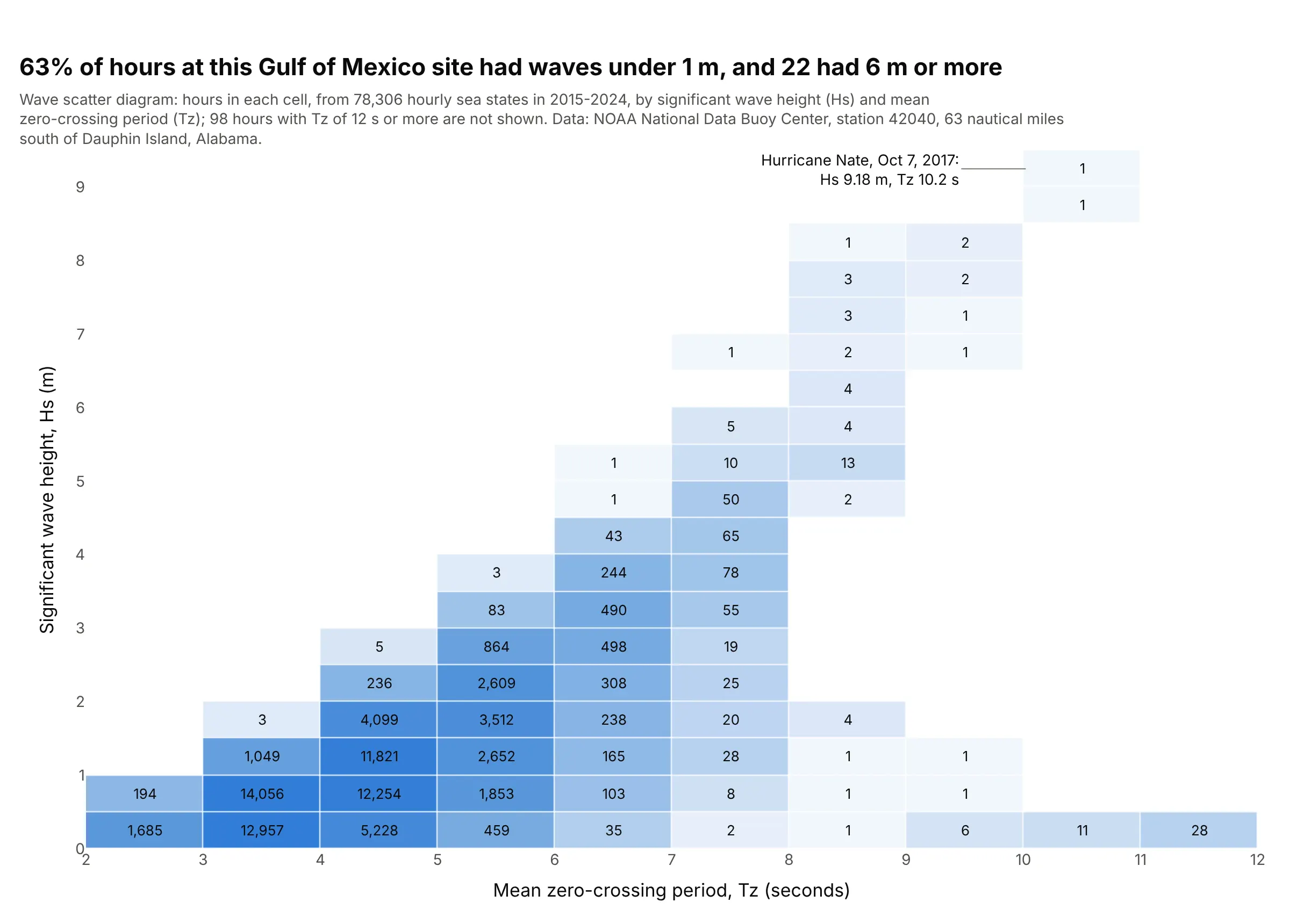
Offshore engineers size platforms and plan vessel operations from a scatter diagram, the hours a site spends in each cell of significant wave height (Hs) and mean zero-crossing period (Tz). At this Gulf of Mexico buoy, 63% of 78,306 hours had waves under 1 m and 22 hours had 6 m or more, the highest 9.18 m during Hurricane Nate in 2017. Data: US National Oceanic and Atmospheric Administration (NOAA), National Data Buoy Center, station 42040.

Tip: print the count in every filled cell and leave the empty ones blank, the table layout of offshore standards such as DNV-RP-C205, with a light color scale behind the numbers.

6. Exoplanet masses and orbits

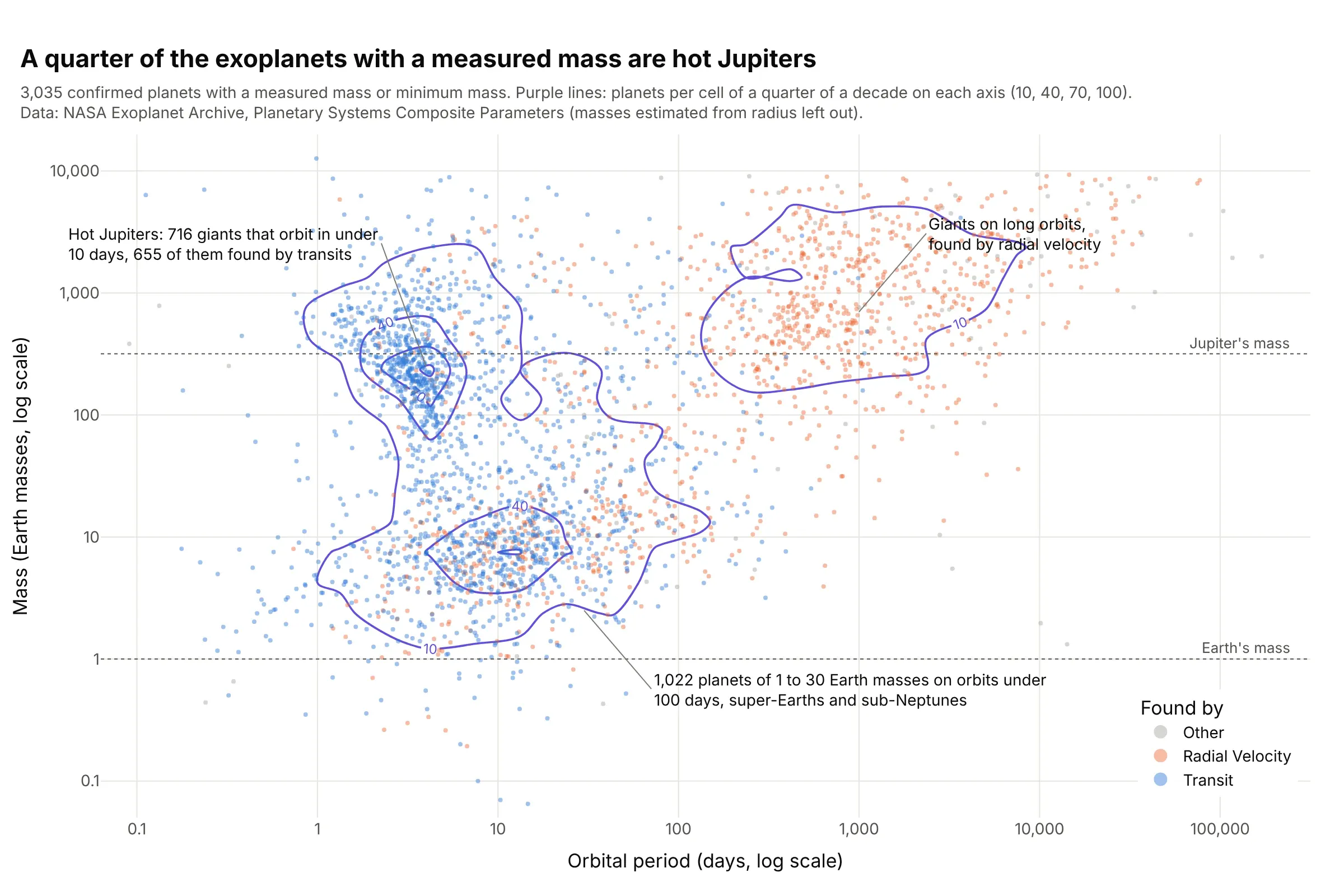
Of 3,035 exoplanets with a measured mass, 716 (24%) are hot Jupiters, giants that orbit in under 10 days, and 655 of those were found by transits, which favor big planets on short orbits. The contour lines show three crowds, and the dot colors show how much each owes to the detection method. Data: NASA Exoplanet Archive, Planetary Systems Composite Parameters.

Tip: bin the log10 of both variables and relabel the ticks as real numbers, because Plotly’s histogram bins are linear even on a log axis.