3D Surface Plots - A Complete Guide

TL;DR

• A 3D surface plot draws a value measured over a grid of two variables (z over x and y) as a sheet, so the shape of the whole grid is visible at once: ridges, valleys, slopes and cliffs.
• 3D surface plots are also known as surface plots, surface charts and 3-D surface charts, and are similar to contour plots and heatmaps.
• Use one when the shape is the point: terrain, volatility surfaces, yield curves over time, dose-response matrices, power output by hour and day.
• 3D hides whatever sits behind a peak and makes exact values hard to read, so choose the camera on purpose, add contour lines, and pair the surface with a heatmap or line chart when readers need numbers. Interactive HTML, where readers can rotate it, is where a surface works best.
• Any coding agent can make one with Plotly in a minute. In Python it's go.Figure(go.Surface(z=grid)).

What is a 3D surface plot?

3D surface plots look like this:

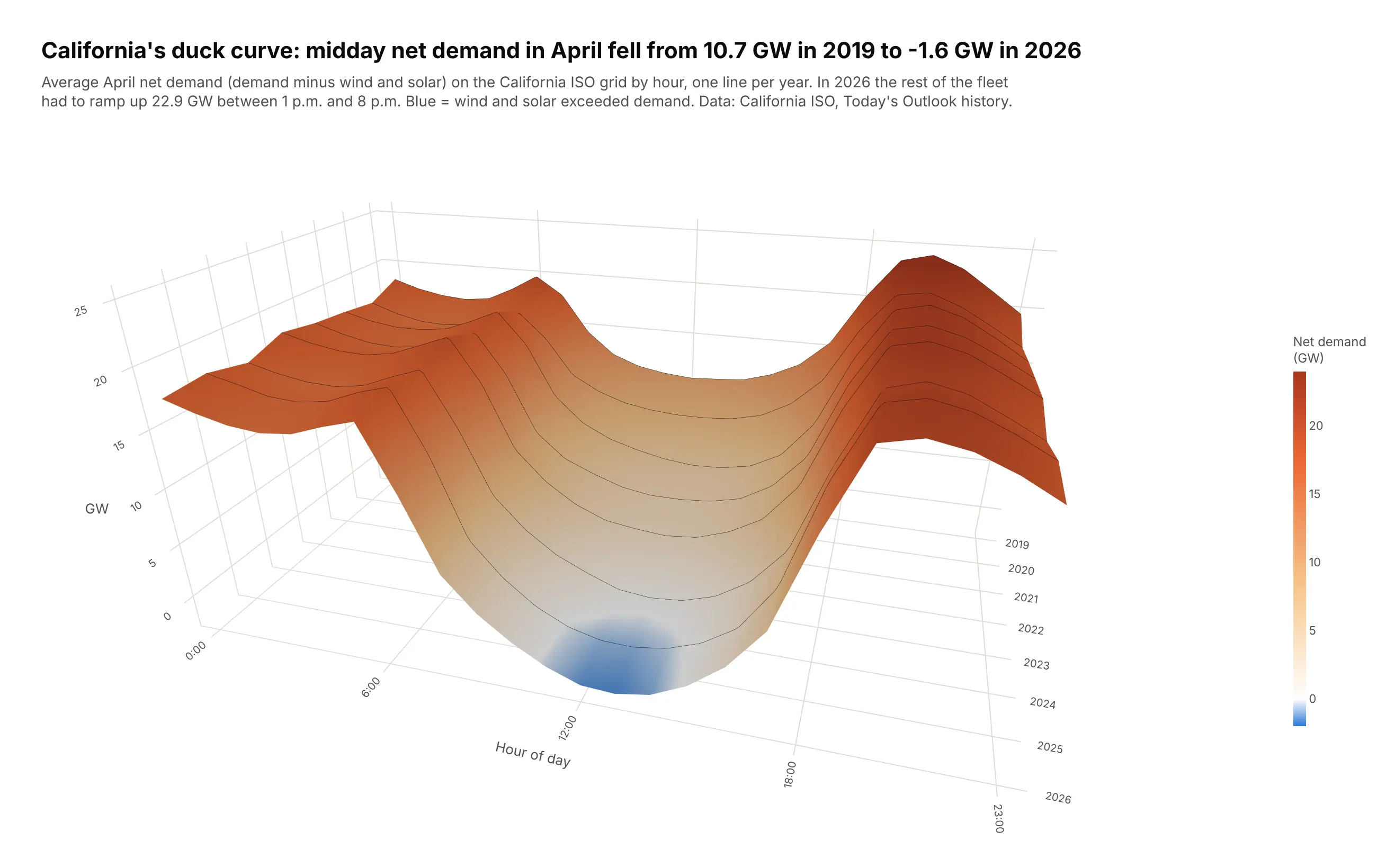
Data: California ISO, Today's Outlook history.

How do you read a 3D surface plot? In the example above, notice these things:

• The two flat axes are the grid the data lives on, with the hour of day running left to right and the year running from the oldest at the back to the newest at the front. Each thin black line across the surface is one year's average April day on the California grid.
• The height of the surface is net demand, the power other plants still had to supply after wind and solar. Color repeats the height, so the orange ridges are the night and evening hours and the pale middle of the day is where wind and solar cover more than half of the load.
• Reading from back to front shows the change over time. The midday valley gets deeper every year, which is the "duck curve" growing as wind and solar cover a larger share of the midday demand each year.
• The blue patch at the front of the valley is where net demand went below zero, meaning wind and solar produced more than all of the demand. It first shows up at midday in 2025.
• Watch out for perspective, because a 3D view makes rows near the front look bigger and can hide low points behind high ones. Use the colorbar, or hover over the surface in an interactive version, for exact values such as the 2026 evening ramp that the subtitle puts at 22.9 GW.

It's often used for charts like these:

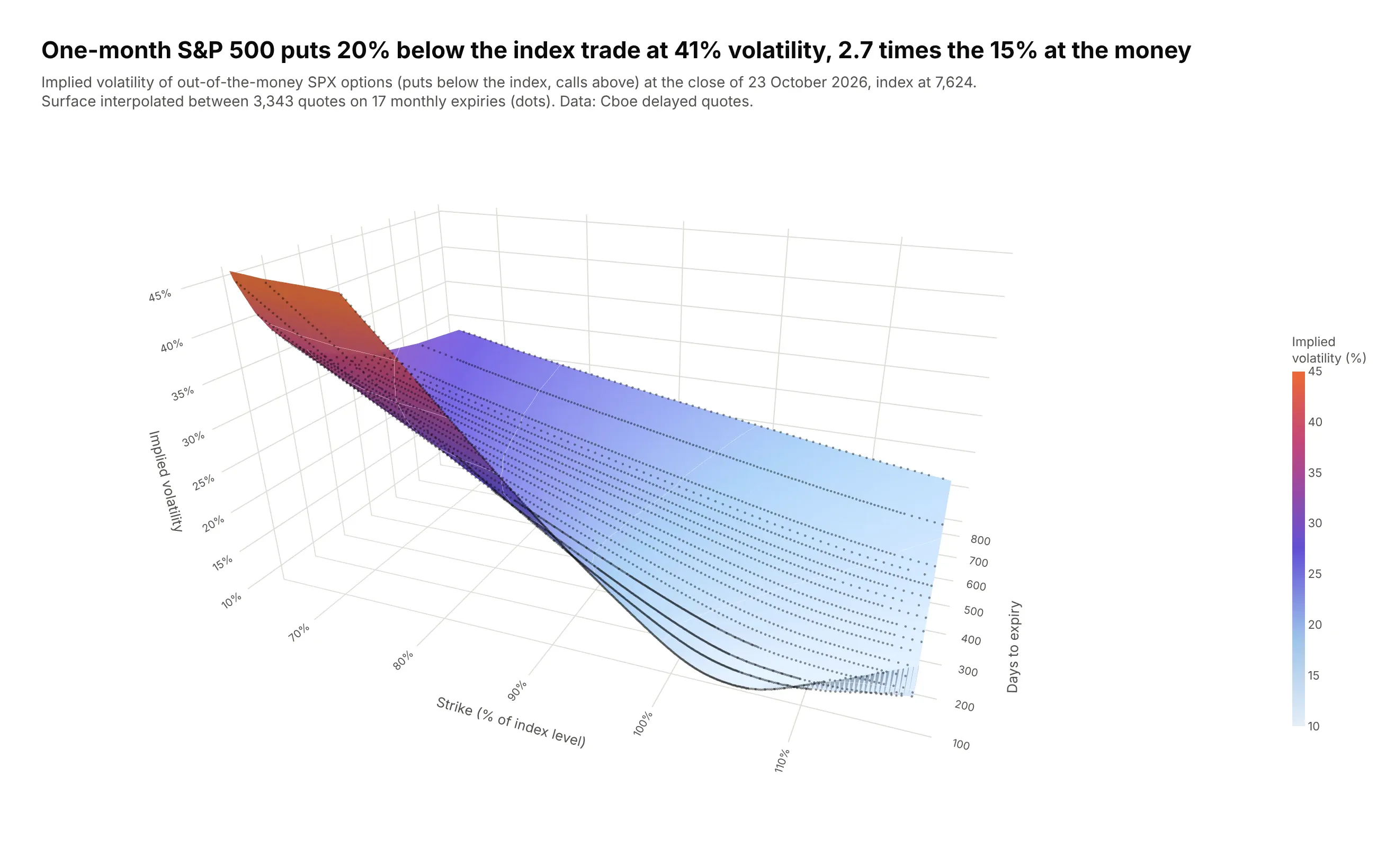
An implied volatility surface. One-month S&P 500 puts 20% below the index traded at 41% implied volatility on 23 October 2026, 2.7 times the 15% at the money. Data: Cboe delayed quotes for SPX options.

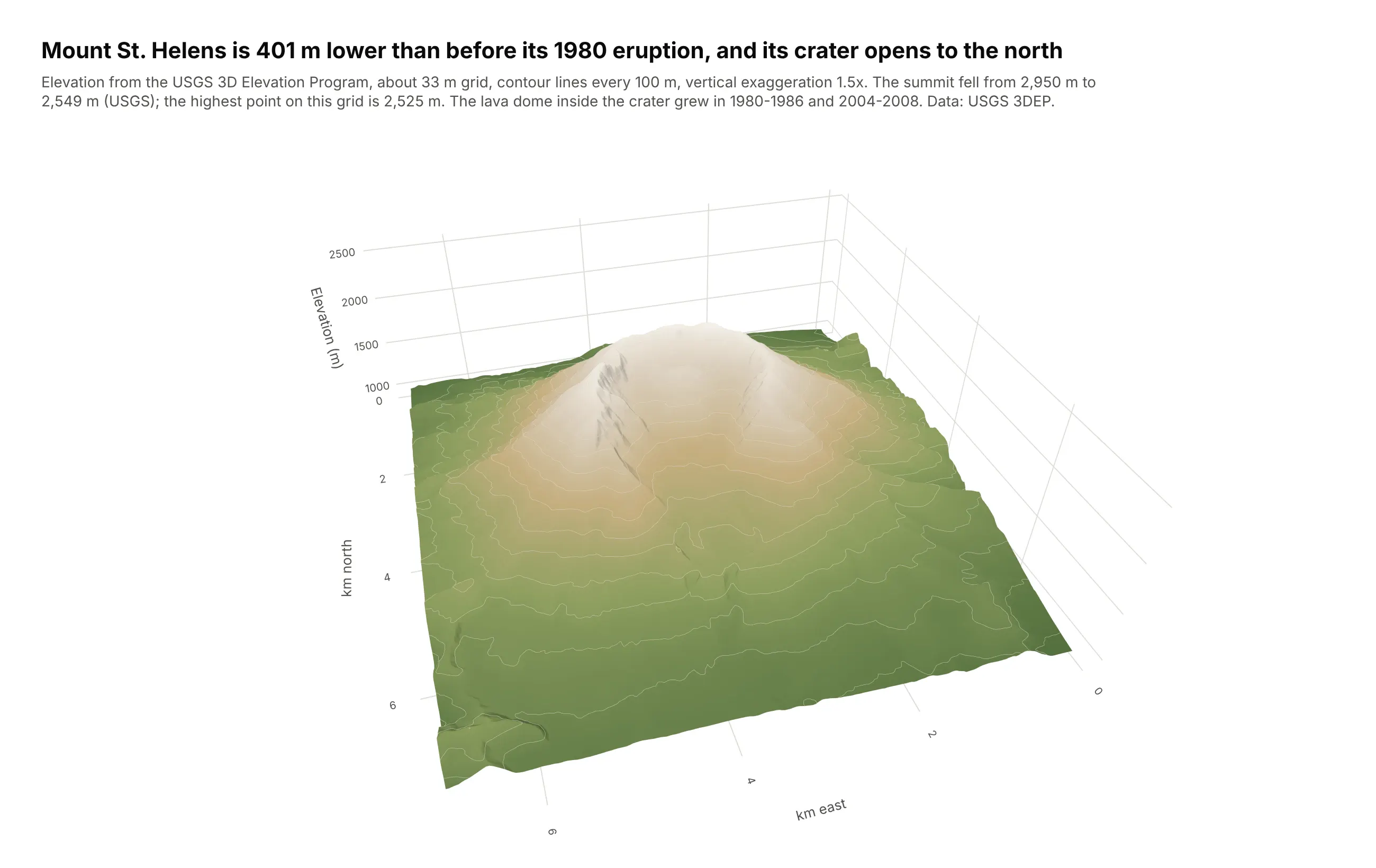
Terrain. Mount St. Helens is 401 m lower than before its 1980 eruption (USGS), and its horseshoe crater opens to the north. Data: USGS 3D Elevation Program.

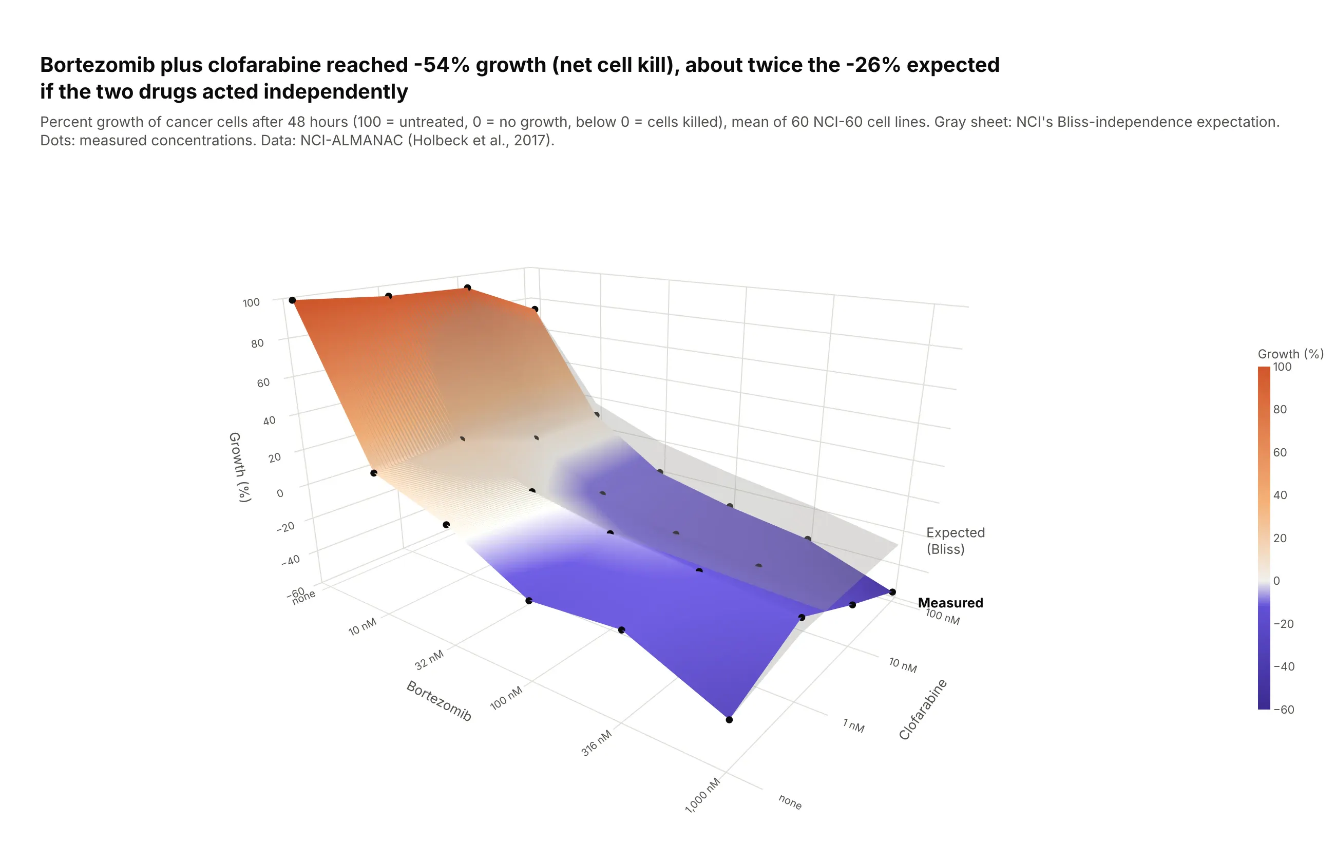
A dose-response surface. At the highest doses, bortezomib plus clofarabine brought average cancer cell growth to -54% (cells killed), about twice the -26% expected if the two drugs acted independently. Data: NCI-ALMANAC (Holbeck et al., 2017).

A short history

In 1879 the Italian statistician Luigi Perozzo drew Sweden's census population for 1750 to 1875 as a 3D surface of age by year, one of the best-known early stereograms of statistical data (Friendly and Denis, Milestones). Here is his layout redrawn with Plotly on Statistics Sweden's single-age series, which starts in 1860:

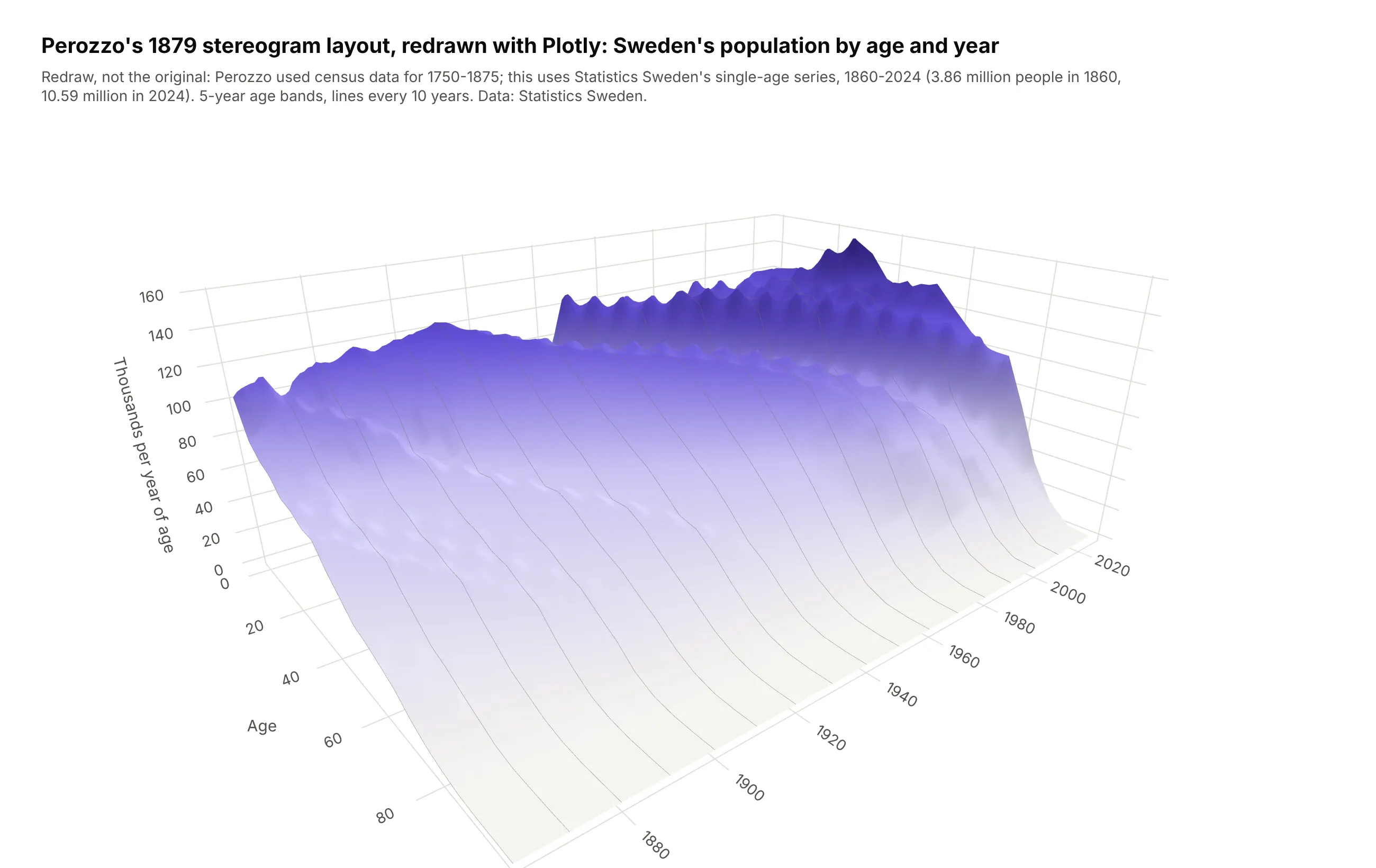
Depth has a mixed record since then. When Michael Siegrist tested pie and bar charts with and without it, readers judged 3D pie charts less accurately and took longer on 3D bar charts (Siegrist, 1996), so use 3D for grids that really have two dimensions, never to decorate a flat chart.

Alternatives to a 3D surface plot

Here's the same duck curve drawn four ways. Some are better for the question, some worse, some just different:

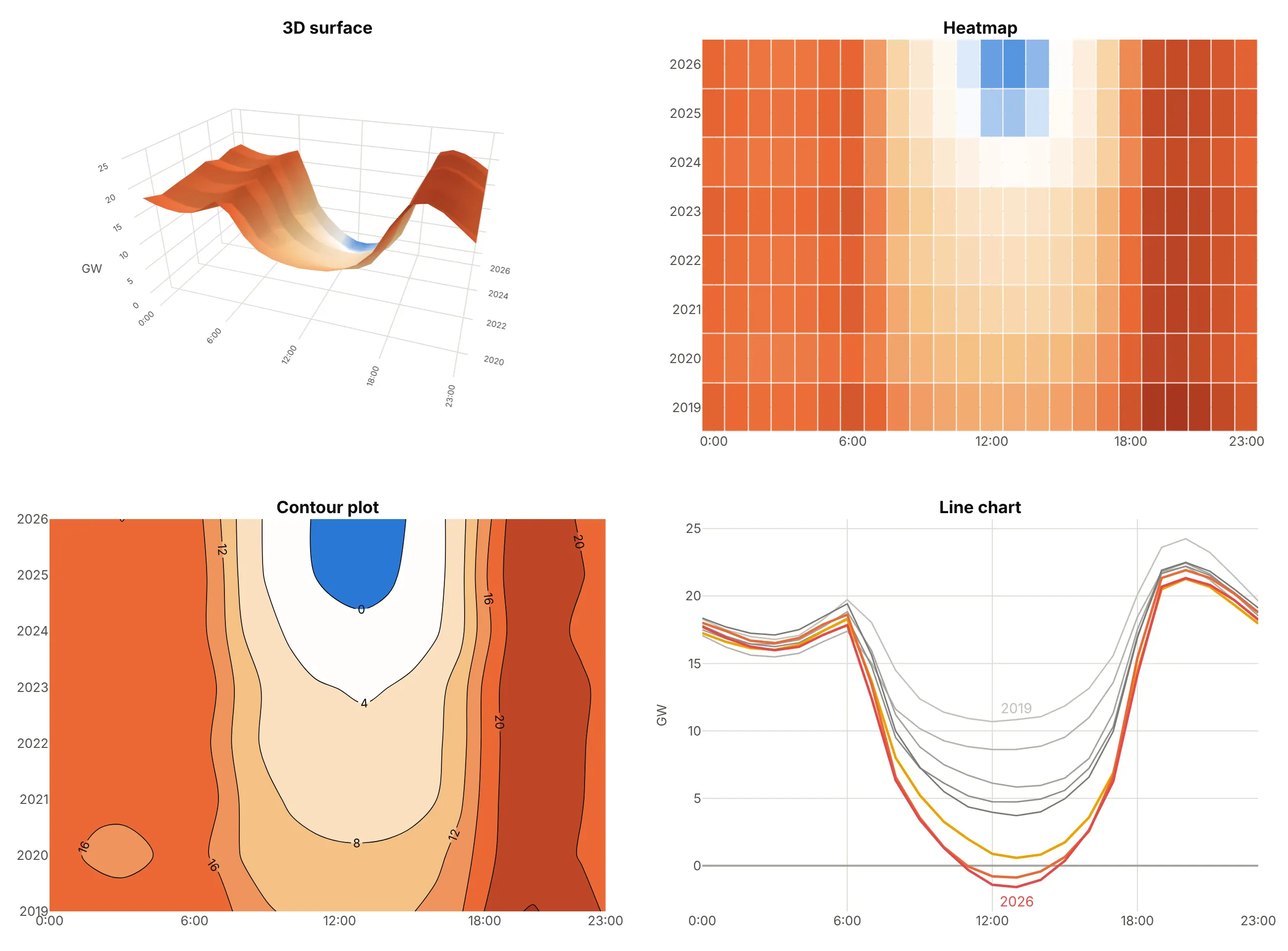
• Heatmap (better for reading values). Every cell is visible and nothing hides behind a peak, though color is less precise than height or position. See our heatmap guide.
• Contour plot (works too). Lines of equal value show where a level is crossed, the way topographic maps show terrain, and you can label them. See our contour plot guide.
• Line chart (better for a few rows). One line per year gives exact values and makes the 2025-2026 drop below zero obvious. Past about ten lines it gets crowded.
• 3D surface (different). It shows the overall shape fastest and is the most engaging, especially when readers can rotate it, but it's the hardest to read precisely.

How to make a 3D surface plot

With AI

ChatGPT, Claude Code, GitHub Copilot, Cursor and other AI tools are excellent at writing Plotly code. Name Plotly in the prompt, say what's on each axis and what the color means, and list the checks you want:

With Plotly Studio

Plotly Studio is a desktop app where you point an AI at a dataset and it builds charts and a Dash app around your questions. Ask for a surface the same way:

Show a 3D surface of hourly solar output by hour of day and day of the year, with a white-to-orange colorscale where zero is white, viewed from the morning side, and a heatmap of the same data next to it.

Make a 3D surface plot in Python or JavaScript

This is the code AI tools write under the hood. In Python, go.Surface needs only a 2D array; this is Mount Bruno's elevation grid from Plotly's documentation:

If your data is in long format, one row per measurement, pivot it first with df.pivot(index="y", columns="x", values="z") and pass the column and index values as x and y.

In JavaScript, plotly.js takes z as an array of rows, one per y value. These are California's April net demand numbers from the chart at the top:

Share it

Every Plotly chart has a Share chart button (the cloud icon in its toolbar) that uploads it to Plotly Cloud and gives you a link. Only you can see it until you change its visibility. For a 3D surface this is the best way to share it, because readers can rotate it and hover for values.

For a live app, put the chart in a Dash app and publish it with the Plotly Cloud CLI. Coding agents can run these commands for you:

If your data has to stay in your own cloud or data center, publish to Dash Enterprise instead.

Dos and don'ts

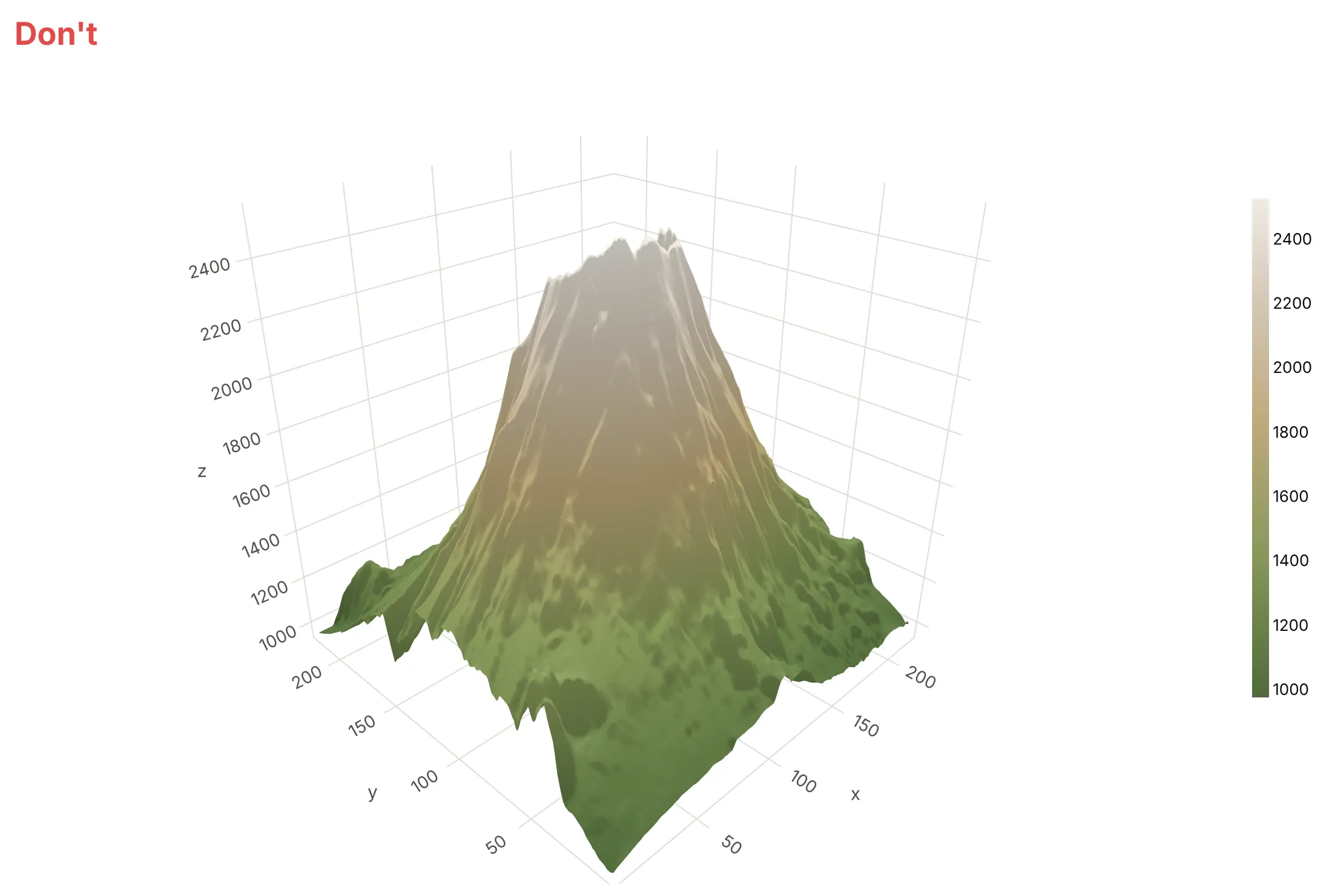
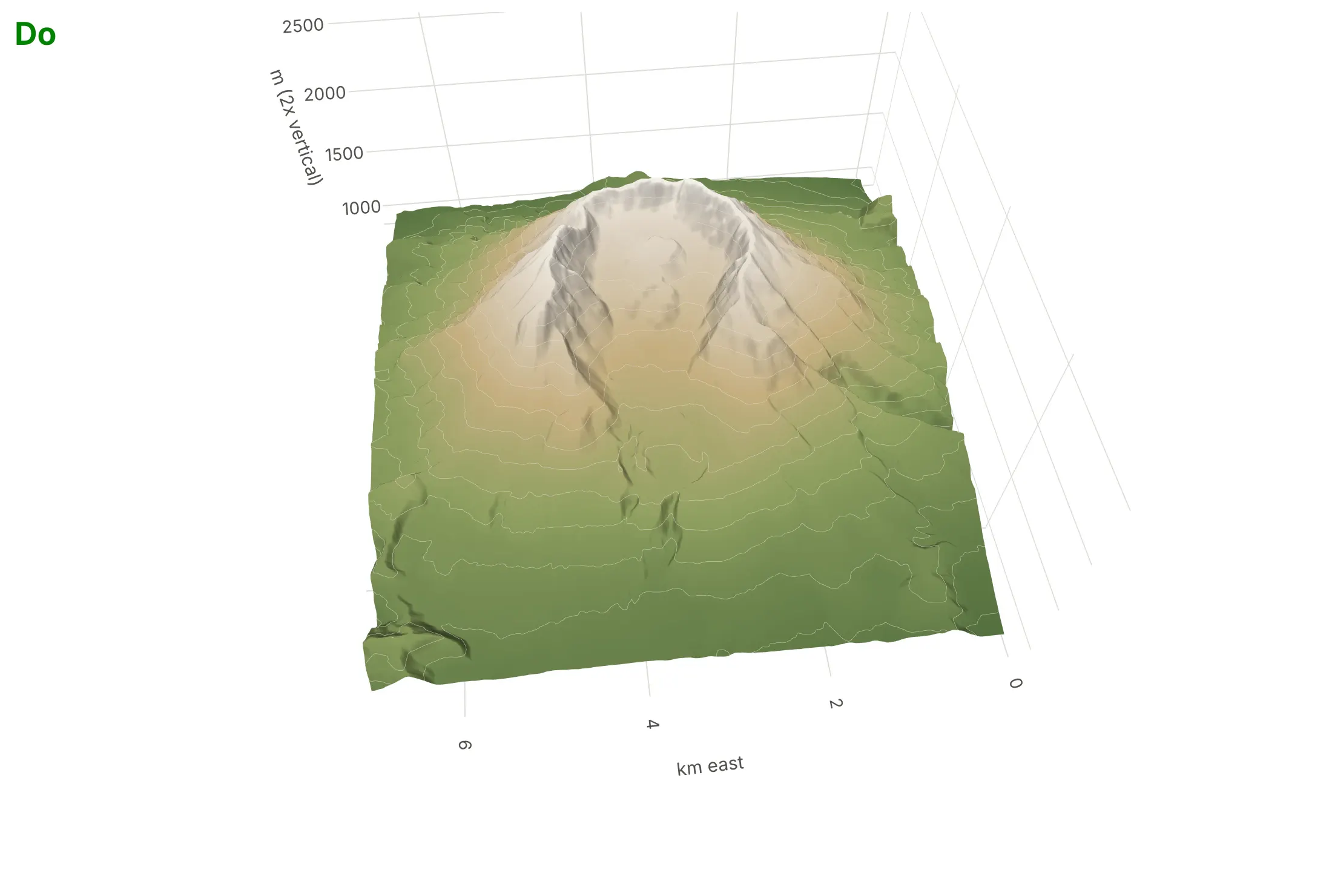
Plotly's defaults are made for exploring, and a surface on its own looks fine until you ask what a reader can actually see. Here is the same Mount St. Helens elevation grid, in the same colors, both ways.

Don't leave the box as a cube, which stretches this mountain about 4.5 times without saying so, label the axes with grid indexes, skip contour lines, or look from the side where the crater is hidden:

Do use real units with true proportions and state any exaggeration, add contour lines, light it softly, and point the camera at the feature that matters:

Choose the camera on purpose

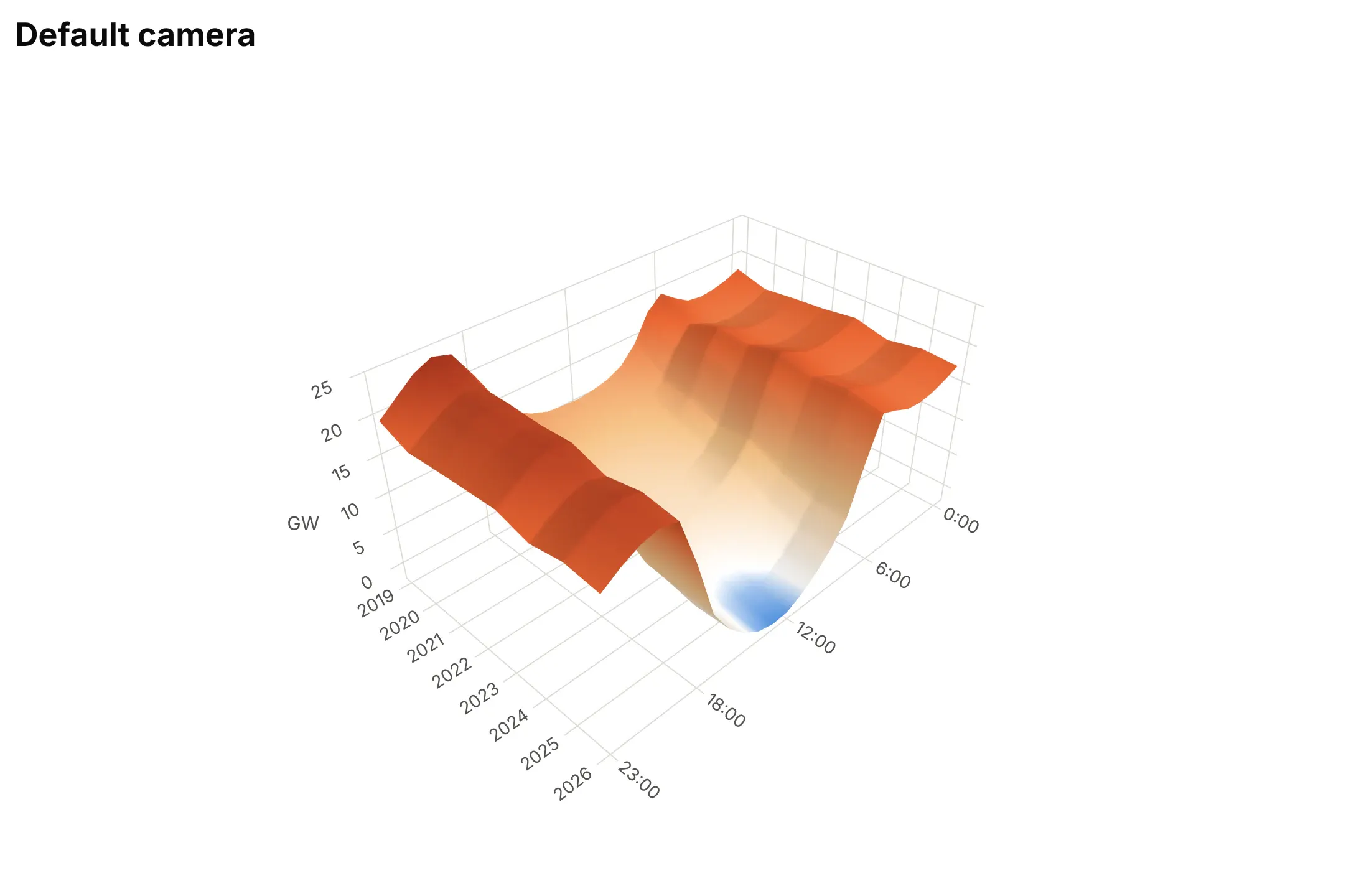
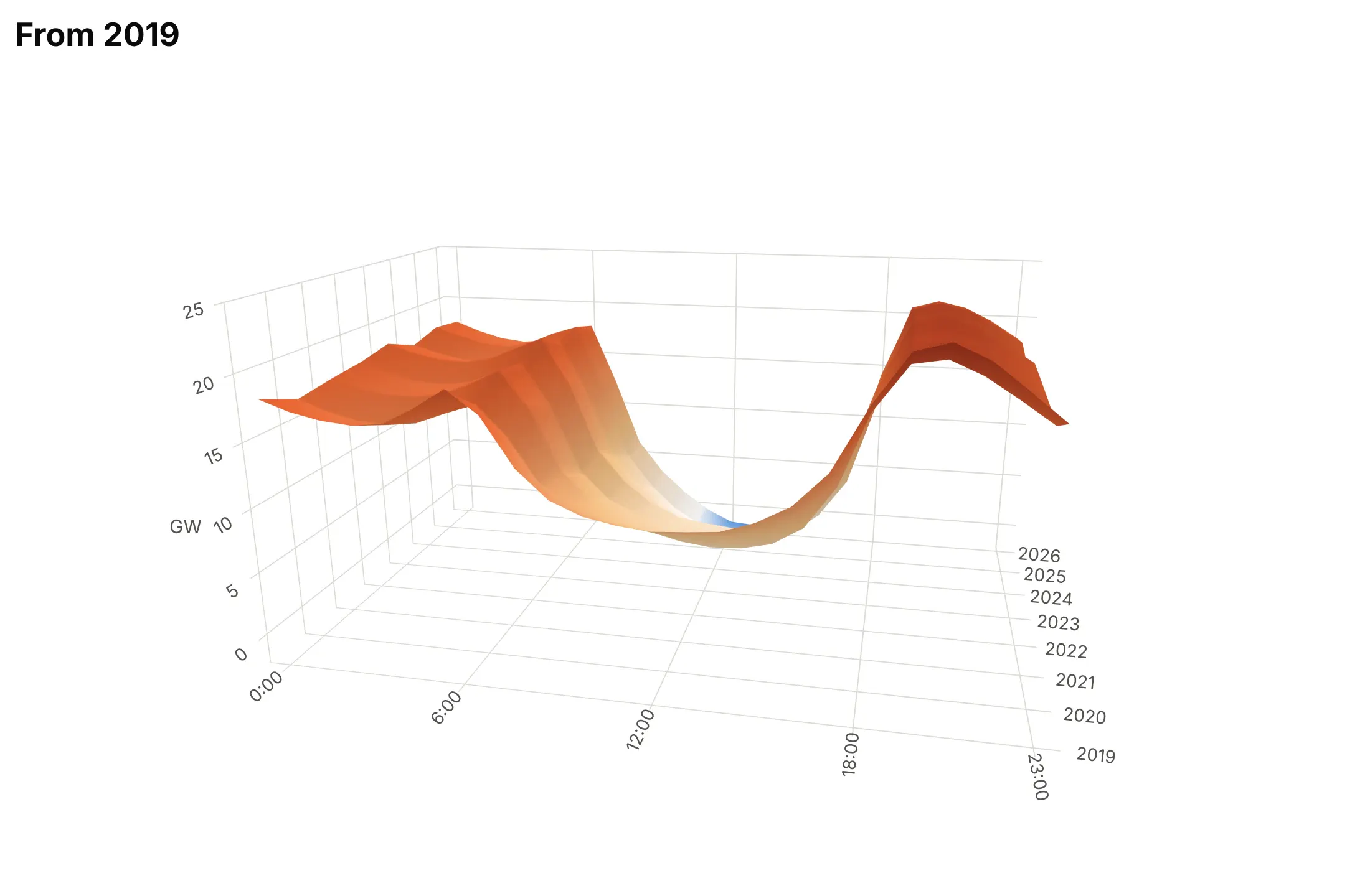
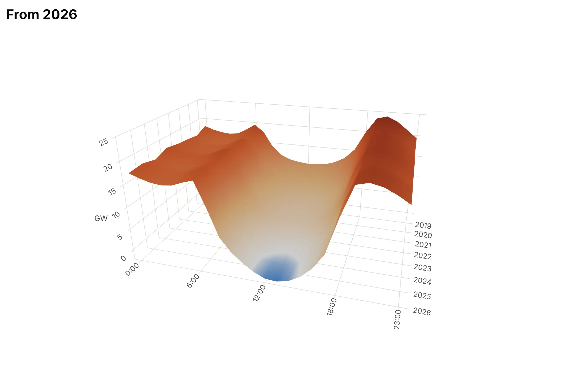
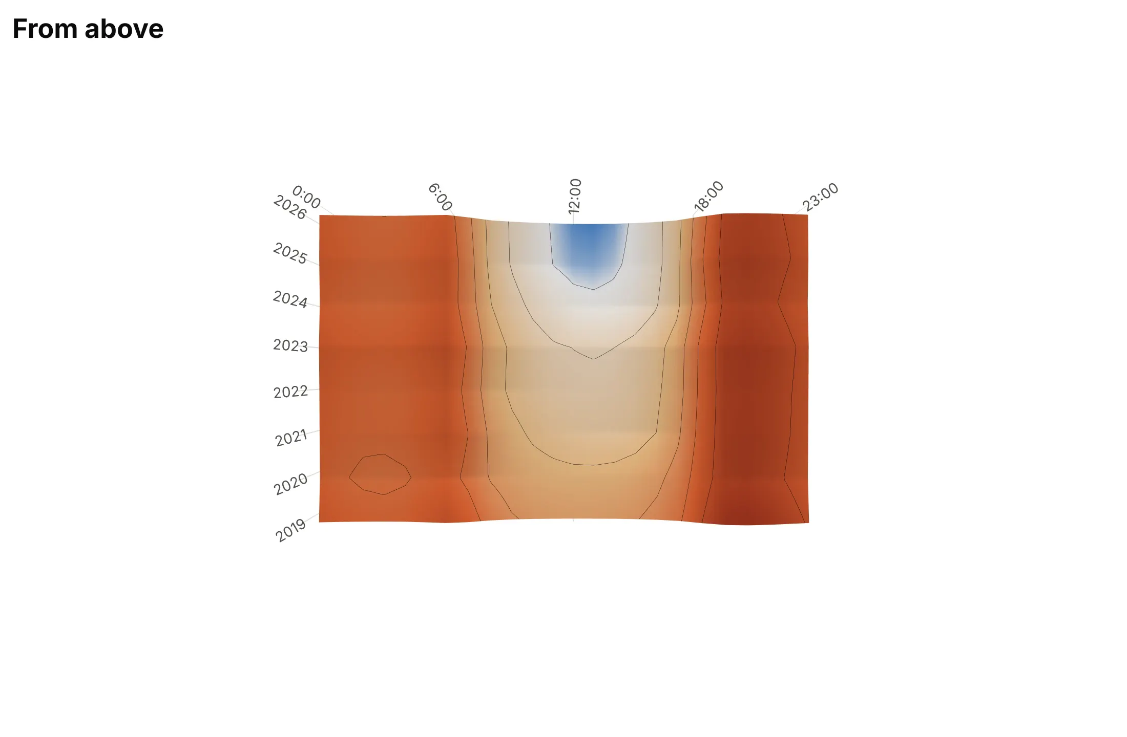
In a static image the camera decides what is in front and what is hidden. Here are four cameras on the duck curve.

Plotly's default angle. It's a reasonable start, but here it looks from the late-evening corner, so time runs away from the reader and the evening ramp overlaps the midday dip.

From 2019 (avoid). The oldest and highest curve is in front, so it hides the deeper recent years.

From 2026, with the x axis reversed (best here). The deepest curve is in front, every year is visible, and the day still runs left to right.

From straight above. The surface becomes a heatmap with contour lines, so nothing is hidden but the shape is gone.

Checklist

Do

• Write a title that states the takeaway with a number.
• Try at least three cameras with scene.camera.eye and keep the one that hides nothing important.
• Set aspectmode="manual" and aspectratio, and state any vertical exaggeration.
• Add contour lines with contours.z, and use surfacecolor when a second variable deserves the color.
• Keep missing cells as NaN so they show as holes, and mark measured points when the surface is interpolated.
• Publish the interactive HTML too, and pair the surface with a heatmap or line chart when readers need numbers.

Don't

• Use a surface when either axis is a category, or for a handful of curves.
• Use a rainbow colorscale such as Jet, which creates false boundaries.
• Trust the default cube, which stretches flat data and squashes tall data.
• Let a peak hide the part of the data that matters.

Options to customize

These are the go.Surface options, and the 3D scene settings around it, that matter most. The full list is in the Plotly 3D surface documentation.

1. z: a 2D array of values, one row per y and one column per x.
2. x, y: the coordinates of the columns and rows; 2D arrays make a parametric surface such as a polar grid.
3. surfacecolor: a second 2D array that sets the color instead of z, for a second variable.
4. colorscale, cmin, cmax, cmid: the color mapping; cmid=0 for signed data, or set cmin and cmax to put a color break at sea level.
5. contours.x, contours.y, contours.z: lines of equal value (show, start, end, size, color, width).
6. contours.z.project.z, usecolormap: copy the contours onto the floor of the box.
7. contours.z.highlight: lines that follow the mouse in the interactive version.
8. hidesurface: draw only the contour lines, for a wireframe look.
9. opacity: transparency, for a second, reference surface.
10. lighting: ambient, diffuse, specular, roughness and fresnel; low specular and high roughness avoid a plastic look.
11. lightposition: where the light comes from, such as the northwest for terrain.
12. hovertemplate, customdata: hover text with units, labels and counts.
13. scene.camera.eye, center, up: the camera position and target.
14. scene.camera.projection.type: orthographic removes perspective, so equal heights look equal.
15. scene.aspectmode, aspectratio: the box proportions.
16. scene.xaxis.type (and y, z): linear, log, date or category; a log z axis suits rates.
17. scene.xaxis.autorange="reversed": flip an axis to keep the reading direction when the camera turns around.
18. scene.annotations: text with arrows anchored to 3D points.
19. go.Mesh3d (x, y, z, i, j, k, delaunayaxis, alphahull, intensity): a surface from triangles or scattered points, for data that isn't on a grid.

More 3D surface plot examples

Ten more surfaces built from real public data, each with its source, the technique that makes it work and a prompt to rebuild it.

1. The US Treasury yield curve since 1982

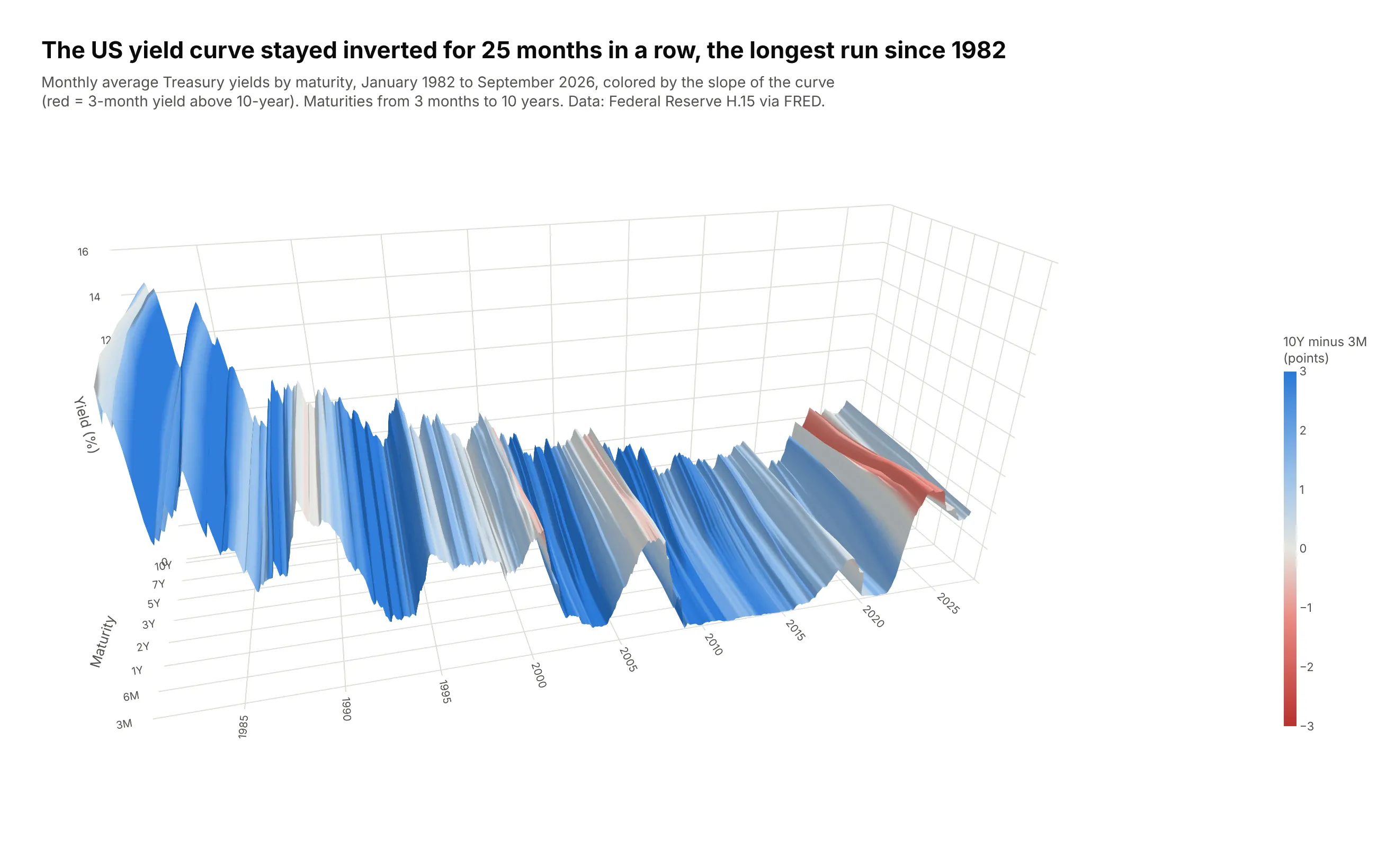
Each of the 537 months is one yield curve from 3 months to 10 years, and side by side they show the 40-year fall in rates and the jump in 2022. The 3-month yield sat above the 10-year for 25 months in a row, from November 2022 to November 2024, the longest run since at least 1982. Data: Federal Reserve H.15 via FRED, monthly averages.

Tip: the color comes from surfacecolor set to the 10-year minus 3-month spread, so every inverted month is a red band whatever its height.

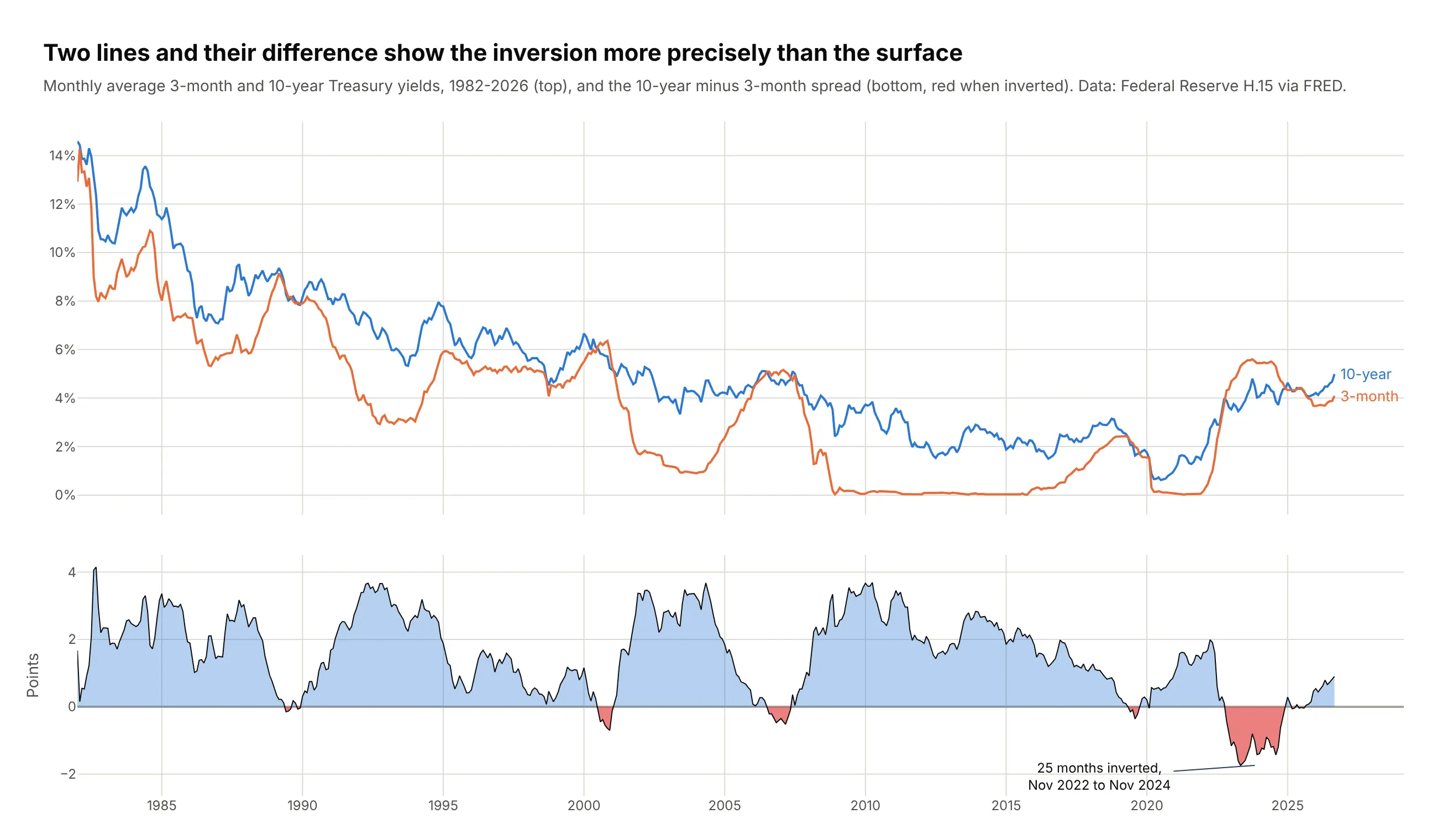
Another way to see it: two lines and their difference read more precisely than the surface. The spread fell to -1.74 points in May 2023, a number the surface can't give you.

2. California's solar output, hour by hour, for a year

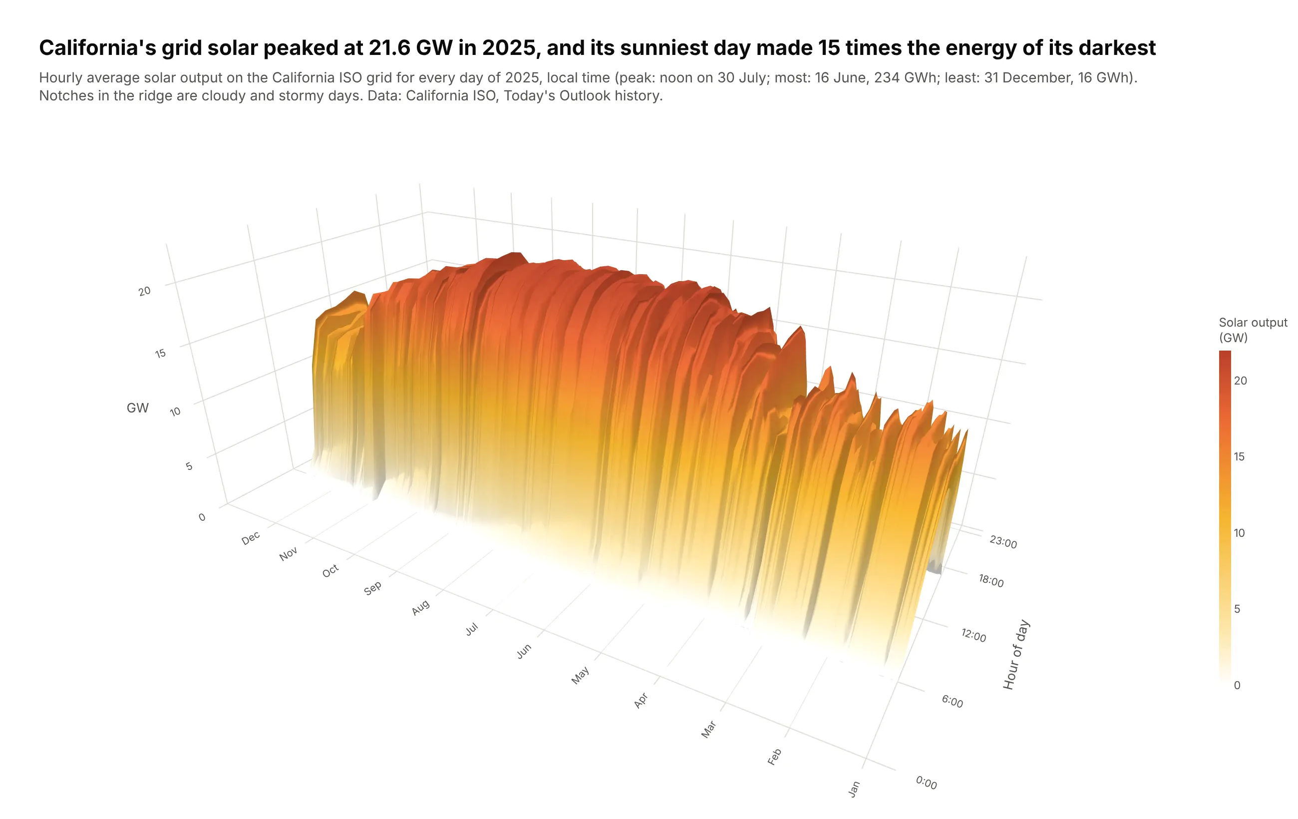
Every day of 2025 is one bell curve of solar output, and together they form a ridge that is wide in summer and narrow in winter. The grid's solar peaked at 21.6 GW at noon on 30 July, and the sunniest day (16 June, 234 GWh) made 15 times the energy of the darkest (31 December, 16 GWh). Data: California ISO, Today's Outlook history.

Tip: the camera looks from the morning side with a light from the same direction (lightposition), so the notches left by storms are shaded.

3. Where a wind farm's energy comes from

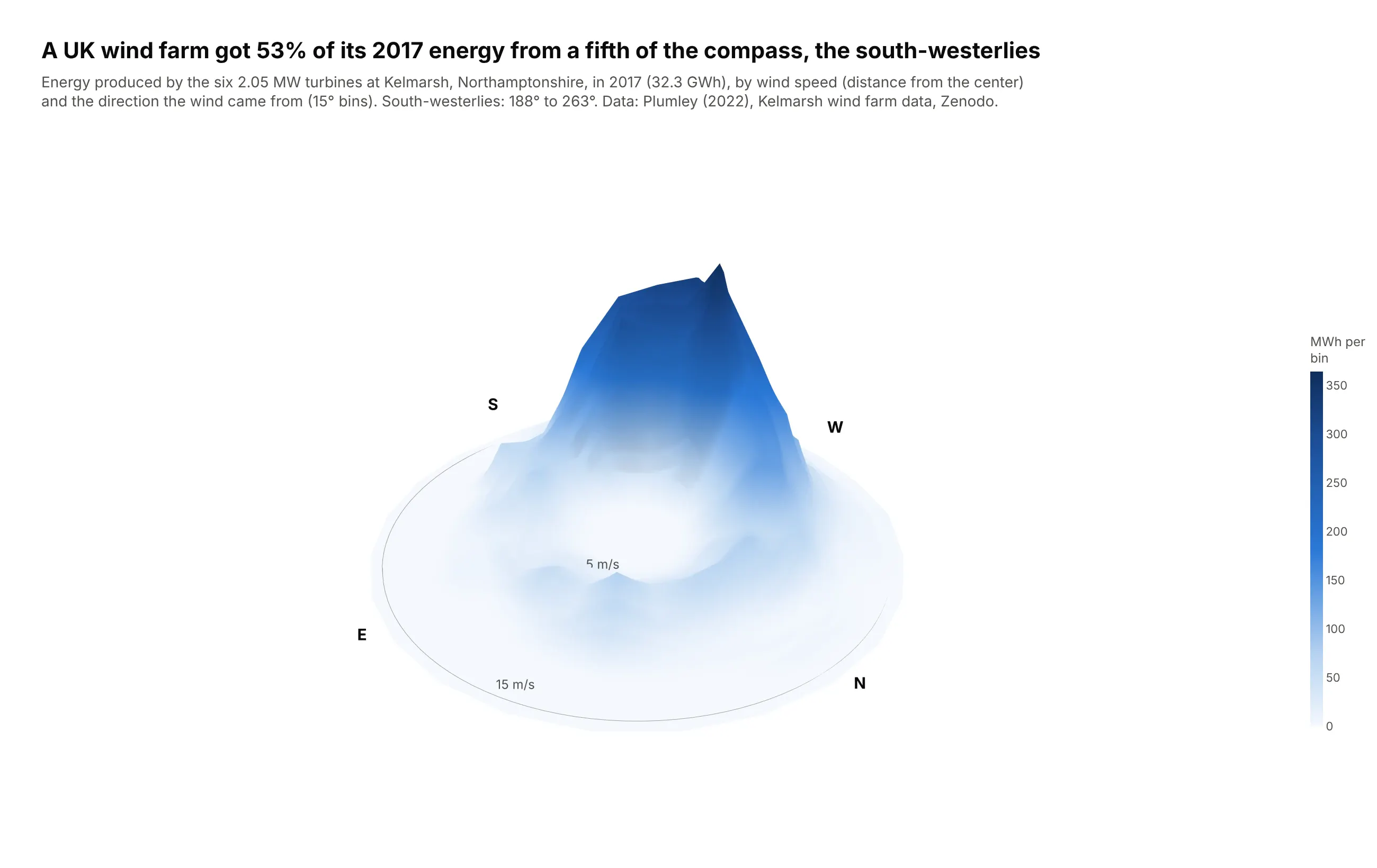
This is a wind rose with height: each cell is the energy the six Kelmarsh turbines produced at that wind speed and direction in 2017. Winds from 188 to 263 degrees, a fifth of the compass, produced 53% of the 32.3 GWh. Data: Plumley (2022), Kelmarsh wind farm data, Zenodo, 10-minute SCADA records.

Tip: a parametric surface, where x, y and z are all 2D arrays (x = speed × sin(direction), y = speed × cos(direction)), draws a polar grid.

4. Every US flu season since 1997

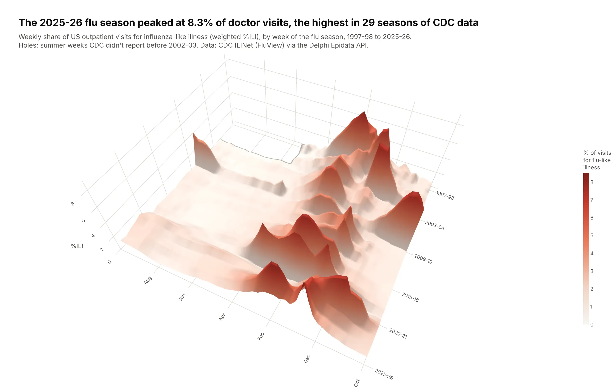
Folding 29 years of weekly data into season by week lines up the winter peaks. The 2025-26 season peaked at 8.3% of outpatient visits in late December, the highest in the record, ahead of 2024-25 (7.8%) and the October 2009 H1N1 pandemic wave (7.7%). Data: CDC ILINet (FluView), weighted %ILI, via the Delphi Epidata API.

Tip: the summer weeks CDC didn't report before 2002-03 are NaN and draw as holes instead of fake zeros.

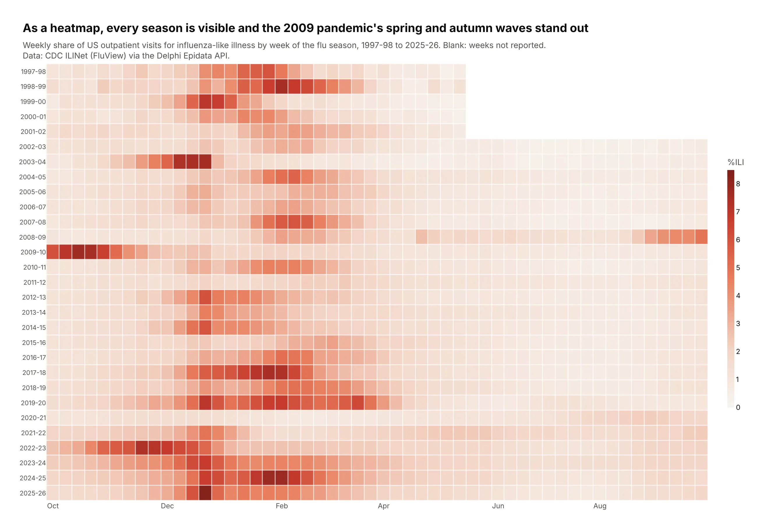
Another way to see it: as a heatmap every season is visible, including the spring and autumn waves of the 2009 pandemic and the flat 2020-21 season.

5. US death rates by age and year

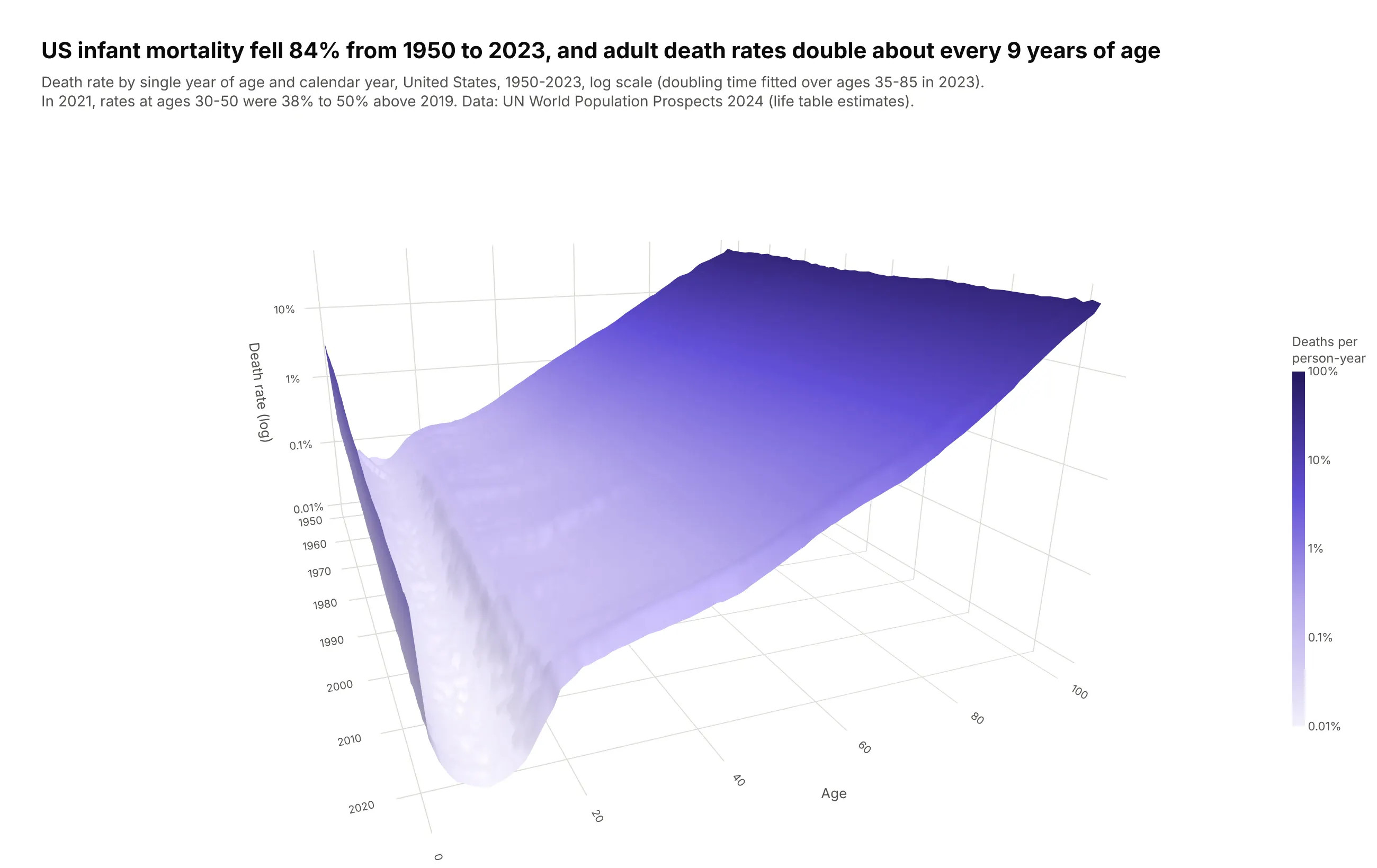
Demographers call this a Lexis surface. US infant mortality fell 84% from 1950 to 2023, and on a log scale adult death rates rise in a straight line, doubling about every 9 years of age. In 2021, rates at ages 30 to 50 were 38% to 50% higher than in 2019. Data: UN World Population Prospects 2024, life tables (estimates).

Tip: rates span four orders of magnitude, so scene.zaxis.type="log" and surfacecolor=np.log10(rate) make equal steps of height and color equal ratios.

6. What makes a batted ball a hit

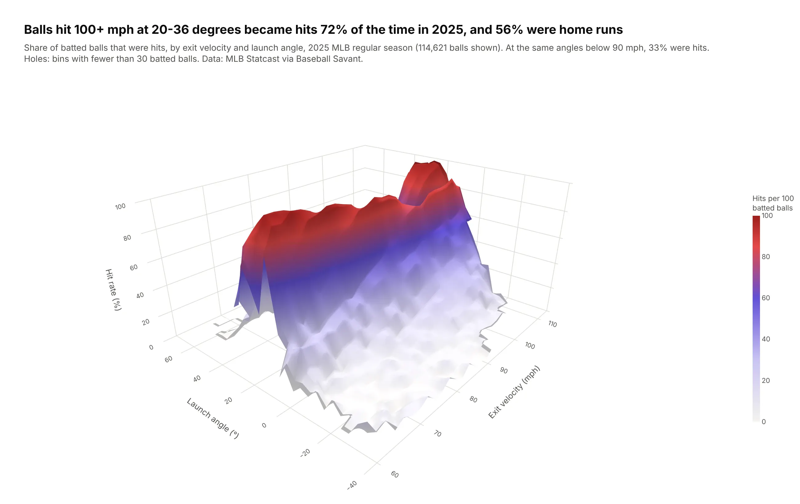
Statcast measures every batted ball's speed and angle, and the chance of a hit rises steeply with both. In 2025, balls hit at 100 mph or more between 20 and 36 degrees became hits 72% of the time and home runs 56% of the time, against 33% hits at the same angles below 90 mph. Data: MLB Statcast via Baseball Savant, 120,216 batted balls.

Tip: bins with fewer than 30 balls are set to NaN, so the surface has holes instead of spikes from three or four batted balls.

7. The Island of Hawai'i from the seafloor

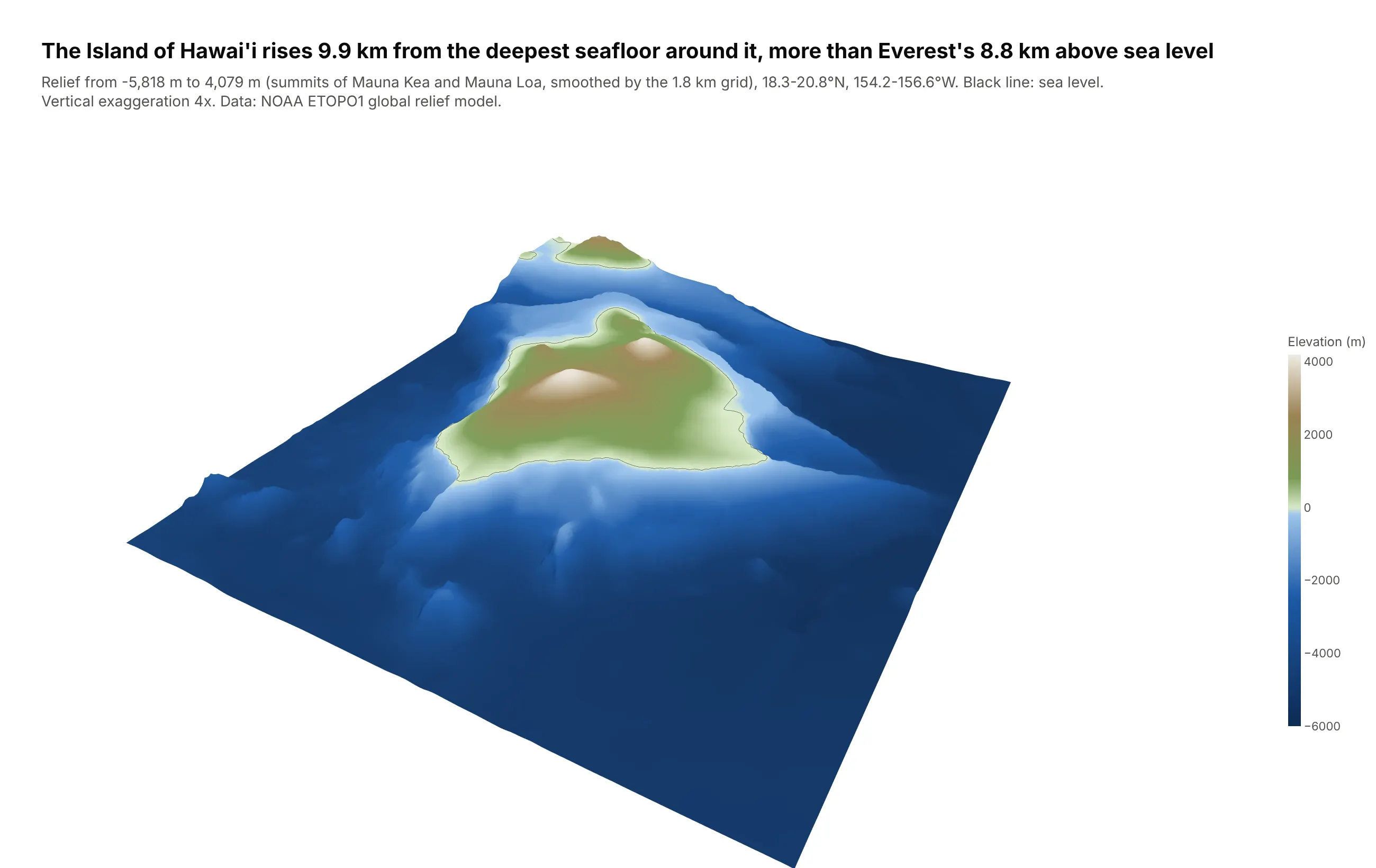
Most of the island is under water. On this grid it rises 9.9 km from the deepest seafloor nearby to the summits of Mauna Kea and Mauna Loa, more than Everest's 8.8 km above sea level, which is why Mauna Kea is often called the tallest mountain on Earth from base to summit. Data: NOAA ETOPO1 global relief model, 1 arc-minute.

Tip: with cmin=-6000 and cmax=4200, the colorscale changes from blues to greens exactly at sea level, and a single contours.z line at 0 draws the coastline.

8. The slab of ocean floor sinking under Tonga

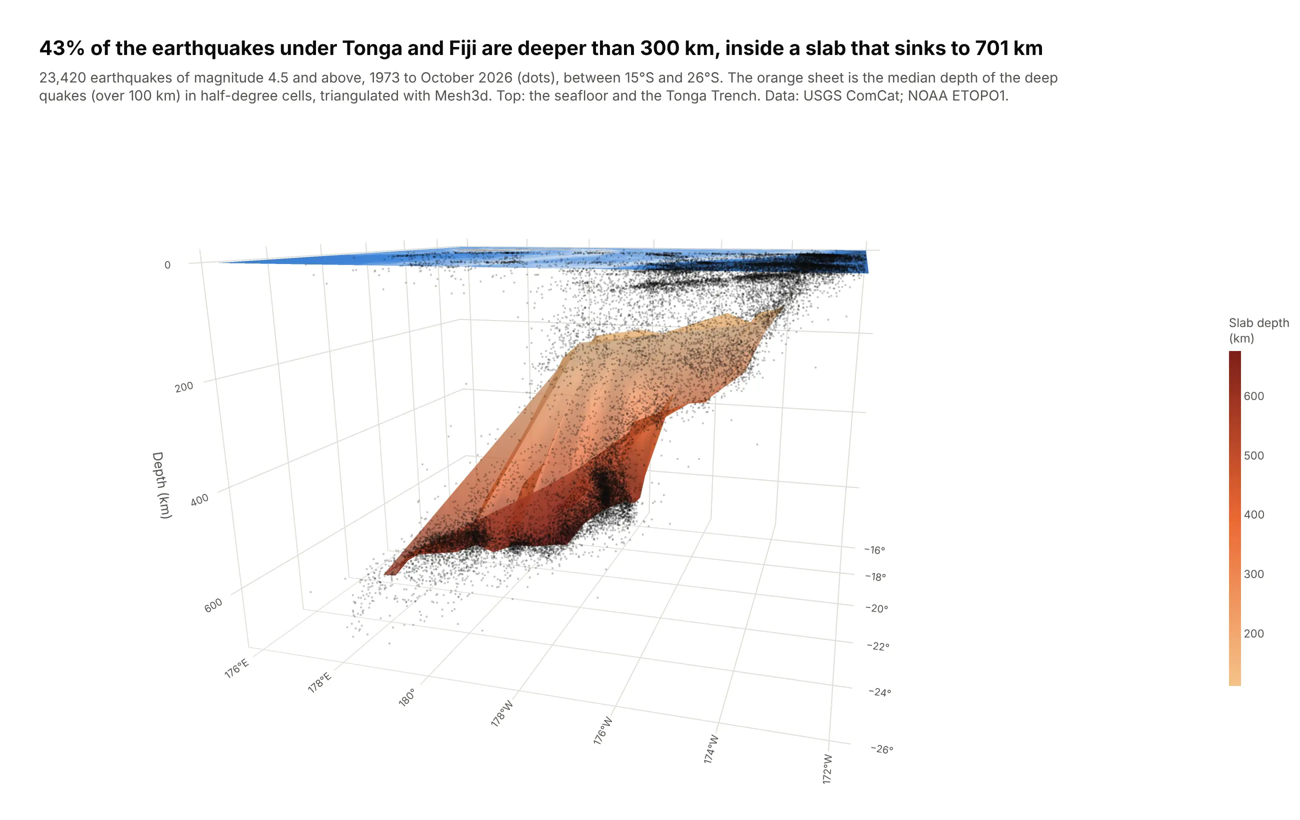
The Pacific plate dives under Tonga at the Tonga Trench, and the earthquakes inside it trace the sinking slab. Of the 23,420 earthquakes of magnitude 4.5 and above recorded since 1973, 43% were deeper than 300 km, and the deepest was at 701 km. Data: USGS ANSS ComCat; NOAA ETOPO1 for the seafloor.

Tip: go.Mesh3d with delaunayaxis="z" triangulates the median depth of the deep quakes in half-degree cells into a sheet, with no grid needed.

9. The Arctic is warming fastest

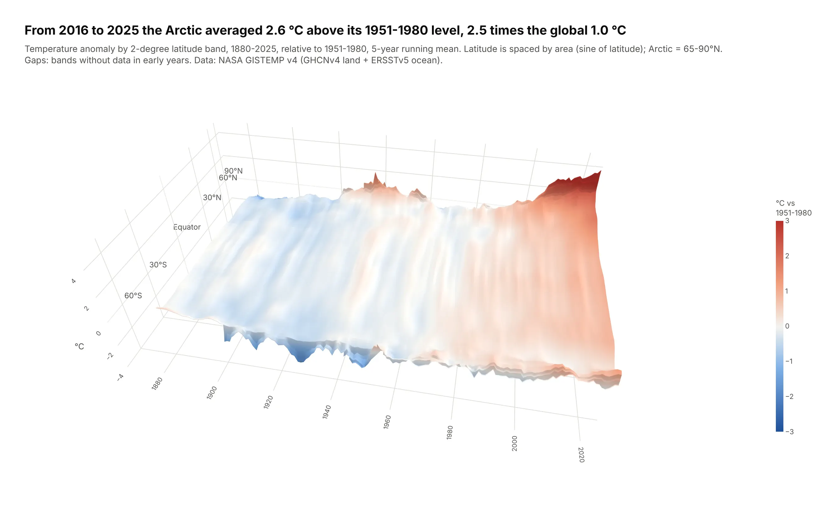
Warming isn't even across latitudes. From 2016 to 2025 the Arctic (65-90°N) averaged 2.6 °C above its 1951-1980 level, 2.5 times the global 1.0 °C, and on the surface the Arctic rises as a wall at the far edge. Data: NASA GISTEMP v4, 2x2 degree grid.

Tip: the latitude axis is spaced by sin(latitude), so each band's width matches its share of the Earth's surface.

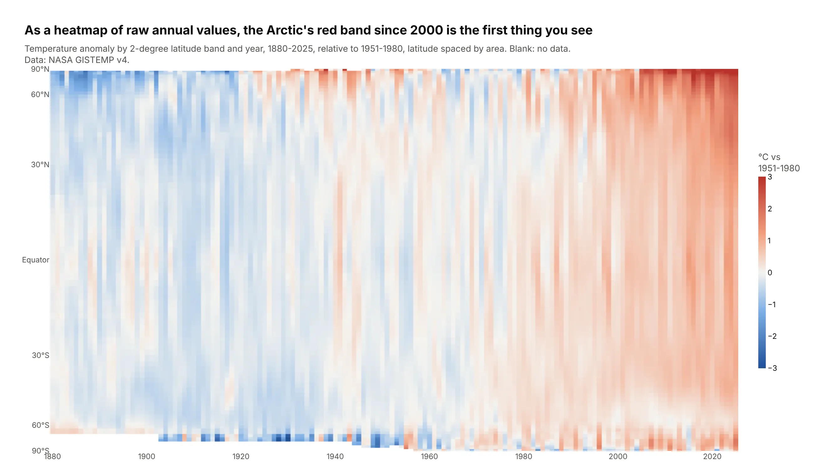
Another way to see it: a heatmap of the raw annual values needs no camera, and the Arctic's red band since 2000 is the first thing you see.

10. The Keeling curve, folded by year

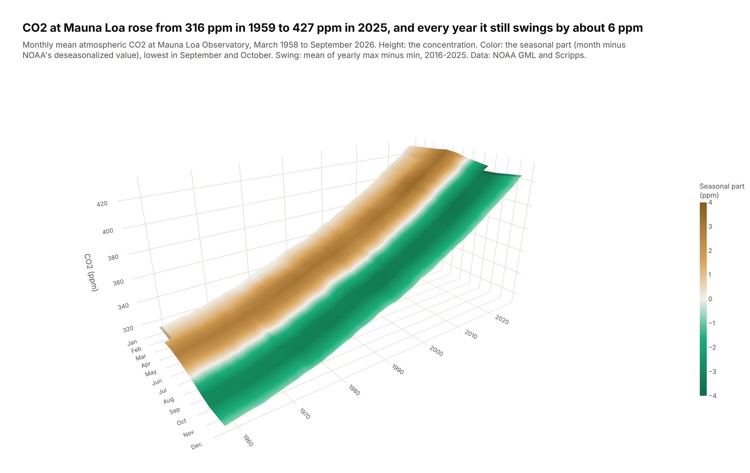
The Keeling curve rises from 316 ppm in 1959 to 427 ppm in 2025, and every year northern forests pull it down by about 6 ppm in summer and release it in winter. Folded into month by year, the trend becomes the slope and the cycle becomes stripes. Data: NOAA Global Monitoring Laboratory and Scripps, Mauna Loa monthly means.

Tip: height is the CO2 level, but surfacecolor is only the seasonal part (each month minus NOAA's deseasonalized value), so one surface shows two things.