Chris Parmer

November 12, 2026

3D Bar Charts - A Complete Guide

TL;DR

A 3D bar chart draws a grid of values as boxes standing on a floor: one axis for each of two categories (or two binned measurements) and the height for the value, so you can rotate it and see the shape of a whole table at once.
3D bar charts are also known as 3D bar graphs, 3-D column charts (Excel), bivariate or 3D histograms (MATLAB's hist3 and histogram2) and, in particle physics, lego plots. They are similar to heatmaps, 2D histograms, 3D surface plots and grouped bar charts.
They work best for a 2D histogram or a map of values on a grid that you can rotate. For a small table of categories over time, a line chart, a heatmap, small multiples or a pair of 2D plots that each show two of the three variables are easier to read, because tall bars hide short ones behind them and perspective changes how tall a bar looks.
You can make a 3D bar chart with Plotly from a go.Mesh3d trace of boxes (8 corners and 12 triangles each), all in one trace: 10,000 bars drew in 0.8 seconds in our test.

What is a 3D bar chart?

3D bar charts look like this:

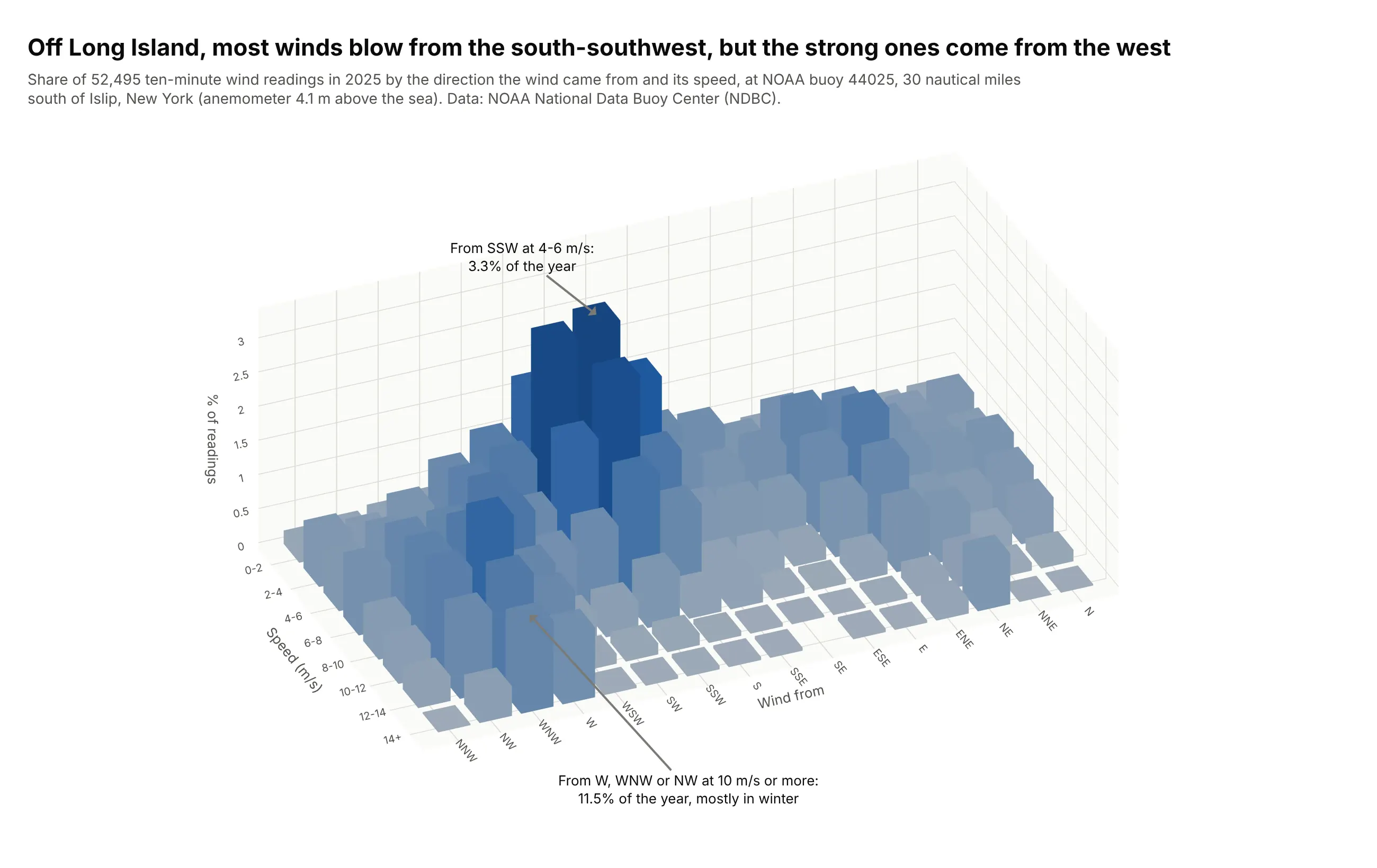
3D bar chart of 52,495 ten-minute wind readings in 2025 at NOAA buoy 44025 south of Long Island, with wind direction in 16 sectors along one axis and speed in 2 m/s bins along the other: the tallest bars are south-southwest winds of 4 to 6 m/s at 3.3% of the year, and a second group of bars for west, west-northwest and northwest winds of 10 m/s or more holds 11.5% of the year, mostly in winter

Data: NOAA National Data Buoy Center (NDBC), station 44025, 30 nautical miles south of Islip, New York, 2025.

How do you read a 3D bar chart? In the example above, notice these things:

The floor is a grid. One axis is the direction the wind came from, in 16 sectors of 22.5 degrees, and the other is its speed in steps of 2 meters per second (m/s). Each bar stands on one cell of that grid, and its height is the share of the year's 52,495 readings that fell in it. Counting readings in a grid of cells like this is called a 2D histogram.
The tallest bar is wind from the south-southwest (SSW) at 4 to 6 m/s, 3.3% of the year. The south, SSW and southwest sectors together hold 28.9% of the readings, at a median speed of 5.6 m/s.
A second group of bars runs toward the strong end of the speed axis in the west, west-northwest and northwest sectors. Winds from there at 10 m/s or more took up 11.5% of the year, and 90% of those readings came between November and March.
The camera looks from the high-speed side so the short bars stand in front of the tall ones. From the other side, the tall south-southwest bars would hide the strong westerlies, which is why a 3D bar chart works best as an interactive chart you can turn.

It's often used for charts like these:

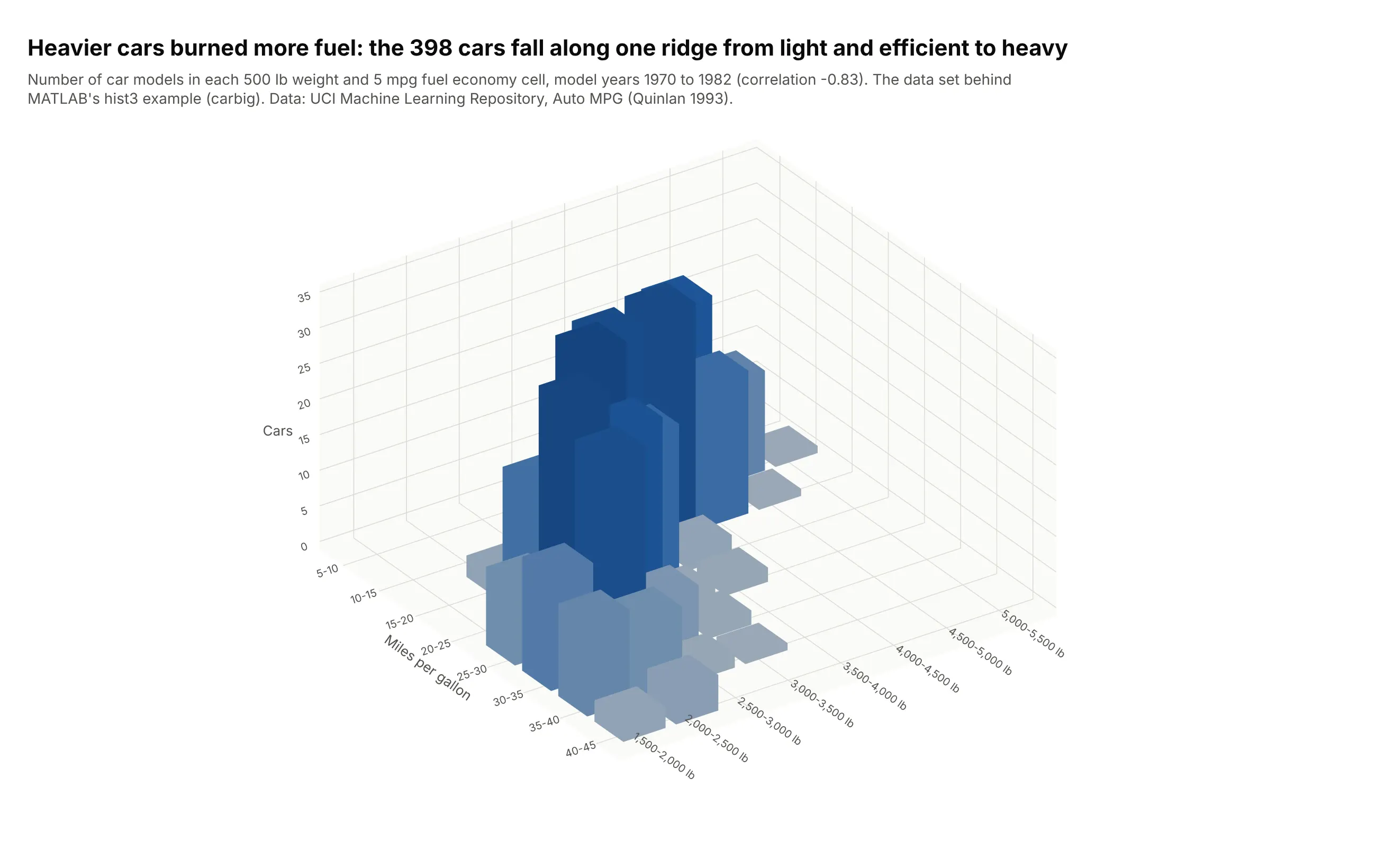
3D histogram of 398 cars from model years 1970 to 1982, counted by weight in 500 lb bins and fuel economy in 5 mpg bins: the bars form one diagonal ridge from light cars at 30 to 40 mpg to heavy cars at 10 to 15 mpg, with the tallest bar of 35 cars at 2,500 to 3,000 lb and 20 to 25 mpg

Two-variable histograms, the classic textbook use. MATLAB's hist3 documentation opens with this data set, the fuel economy and weight of cars from 1970 to 1982, and here the 398 cars fall along one ridge (correlation -0.83). Data: UCI Machine Learning Repository, Auto MPG (Quinlan), the data behind MATLAB's carbig.

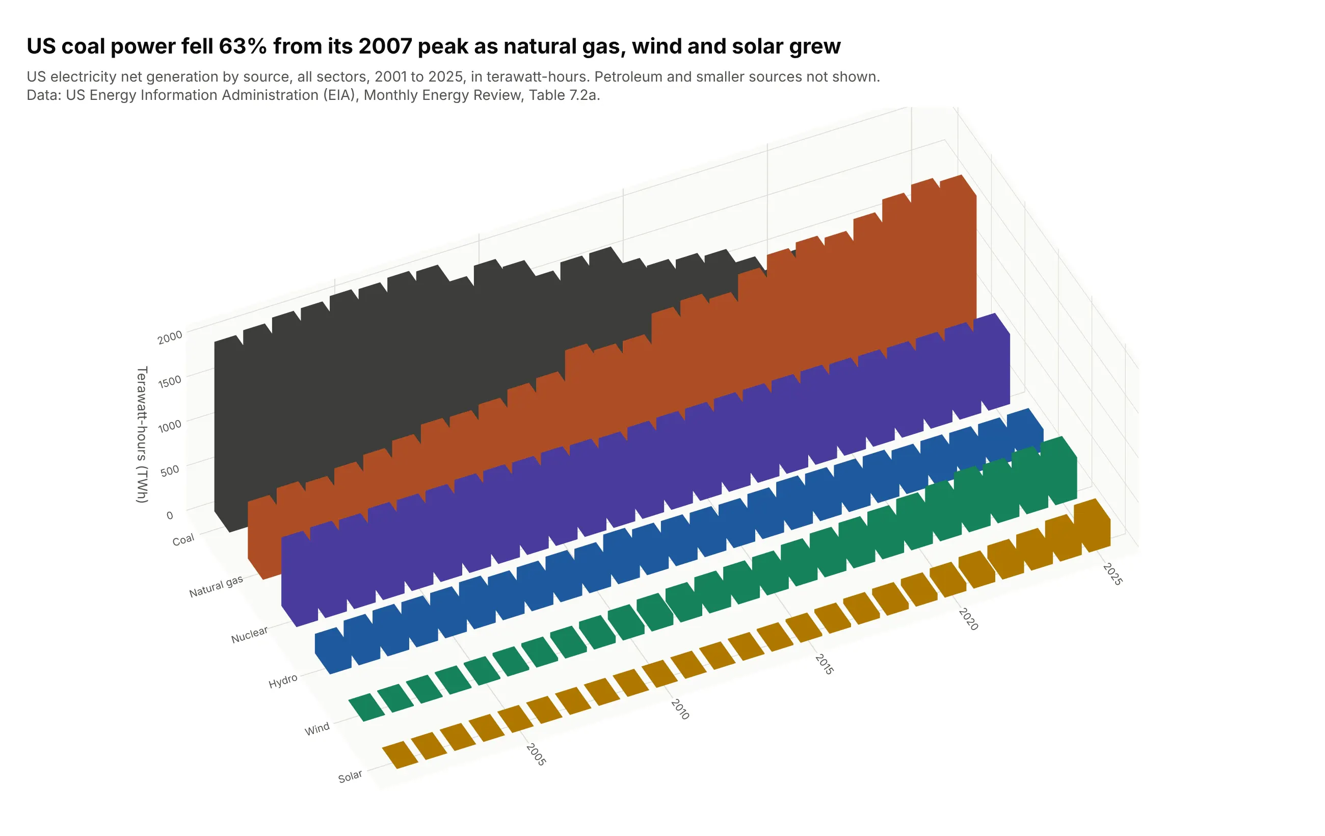
3-D column chart of US electricity generation by source from 2001 to 2025, one row of colored bars each for solar, wind, hydro, nuclear, natural gas and coal: coal falls from about 2,000 terawatt-hours to 737 while natural gas rises to 1,807 and wind and solar grow from almost nothing

3-D column charts of a table, as in Excel. US coal power fell 63% from its 2007 peak to 2025, while natural gas, wind and solar grew. The alternatives section shows the same table as lines, which are easier to read exactly. Data: US Energy Information Administration (EIA), Monthly Energy Review, Table 7.2a.

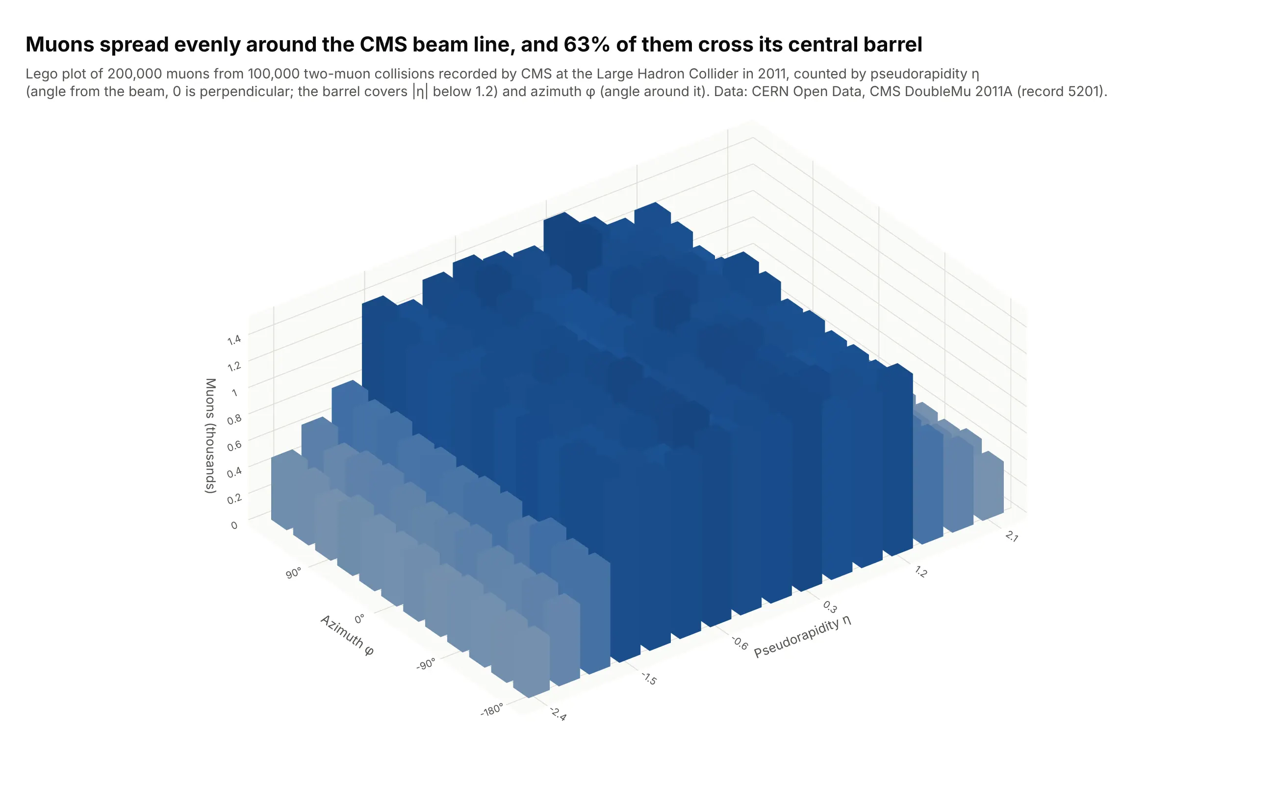
Lego plot of 200,000 muons from 100,000 two-muon collisions recorded by the CMS detector in 2011, counted by pseudorapidity and azimuth: the bars are level all the way around the beam and drop from about 1,300 muons per cell in the center to about 400 at the ends, and 63% of muons are in the central barrel

Lego plots in particle physics. Physicists count particles by pseudorapidity (η, the angle from the beam line) and azimuth (φ, the angle around it), and draw the counts as bars they call a lego plot. Here 63% of 200,000 muons cross the detector's central barrel. Data: CERN Open Data, CMS DoubleMu 2011A, 100,000 two-muon events.

How a 3D bar is built, and why perspective changes its height

A 3D bar chart has two jobs that a flat bar chart doesn't: it has to draw solid boxes in 3D, and it has to project them onto a flat screen. Both shape how you should make and read one.

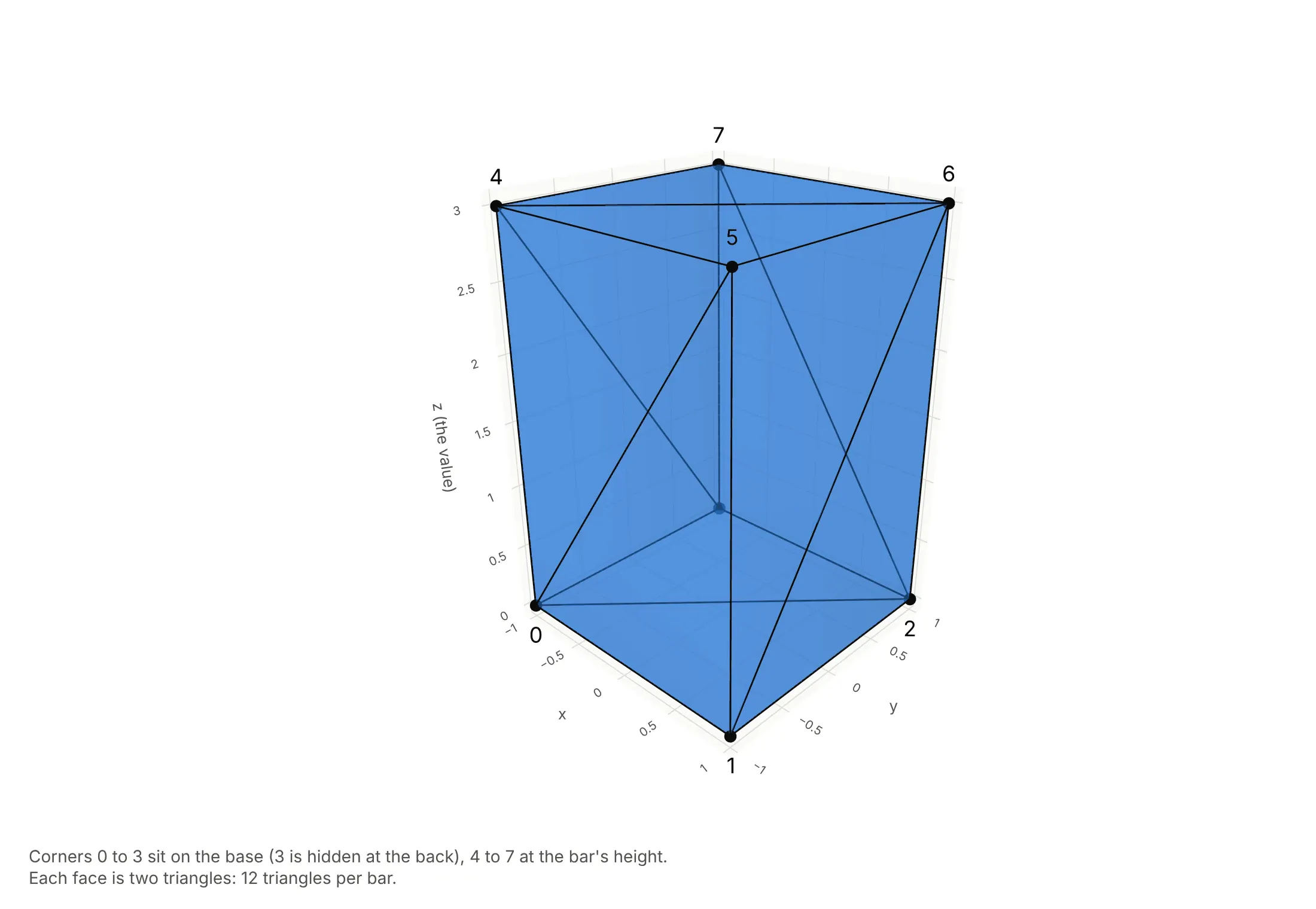
Each bar is a box made of triangles. Graphics cards draw surfaces as triangles, so a box with 6 rectangular faces becomes 12 triangles over 8 corners: 4 on the floor and 4 at the bar's height. Plotly's go.Mesh3d trace takes exactly that, a list of corners and a list of triangles, and the helper in this guide writes them for every bar into one trace:

One 3D bar drawn as a transparent blue box with its 8 corners numbered 0 to 7, corners 0 to 3 on the base and 4 to 7 at the top, and black lines showing the 2 triangles on each of its 6 faces

Perspective makes the back rows look shorter. By default, Plotly's 3D camera uses perspective, like a photograph: things farther away are drawn smaller. That makes 3D scenes look natural, but it also means two bars of the same height are drawn at different heights depending on how far back they stand. An orthographic camera draws every bar at the same scale, so equal values look equal:

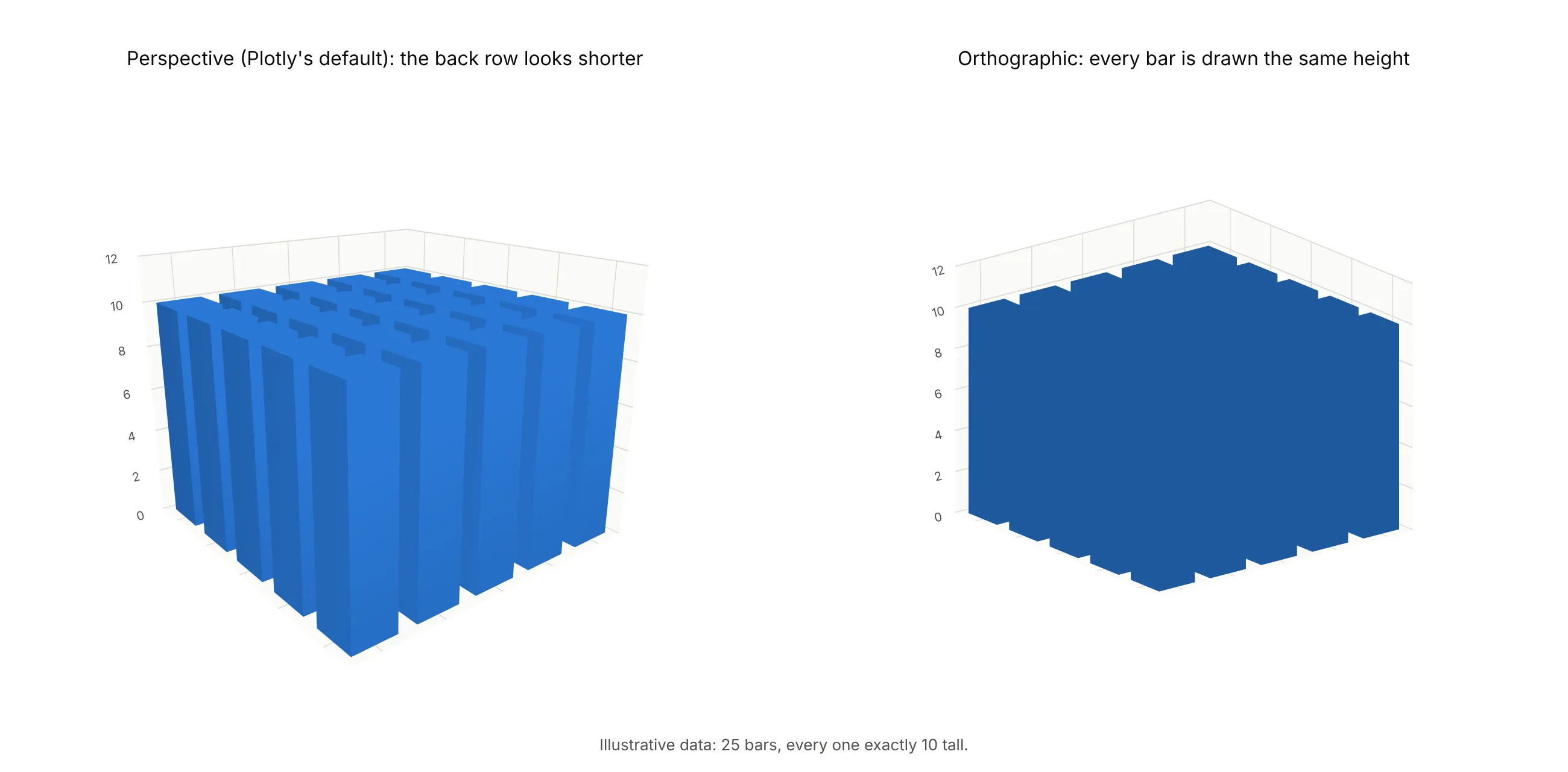
Two views of 25 bars that are all exactly 10 tall: with Plotly's default perspective camera the front bars look much taller than the back row, and with an orthographic camera from the same angle every bar is drawn the same height

Set it with scene_camera=dict(projection=dict(type="orthographic")). Every chart in this guide uses it. Perception studies found the same cost from depth even in simple bar charts: in Zacks et al. (1998) adding 3D depth lowered the accuracy of people's height estimates, although nearby bars distorted them about ten times more, and in Siegrist (1996) and Fischer (2000) people took longer to read 3D bars.

A short history

Bars drawn as boxes in perspective became common with spreadsheet software, and Microsoft Office still lists the 3-D column chart, whose "three axes that you can change (a horizontal axis, a vertical axis, and a depth axis)" compare values "along the horizontal and the depth axes". MATLAB's bar3 ("3-D bar graph") and hist3 date from before 2006, and its newer histogram2 (2015) still draws 3D bars by default. In particle physics, CERN's ROOT library draws any 2D histogram as a lego plot, and its event displays show calorimeter energy as η-φ lego plots. In the 1990s, psychologists tested whether the decorative depth of 3D bars hurt reading (Siegrist 1996, Zacks et al. 1998), which is where most of the advice against them comes from. We couldn't find an early 3D bar chart with public data behind it to redraw, so example 2 above redraws MATLAB's own first hist3 example instead.

Alternatives to a 3D bar chart

Here's the same year of wind readings drawn six ways. Some are better for the question, some worse, some just different:

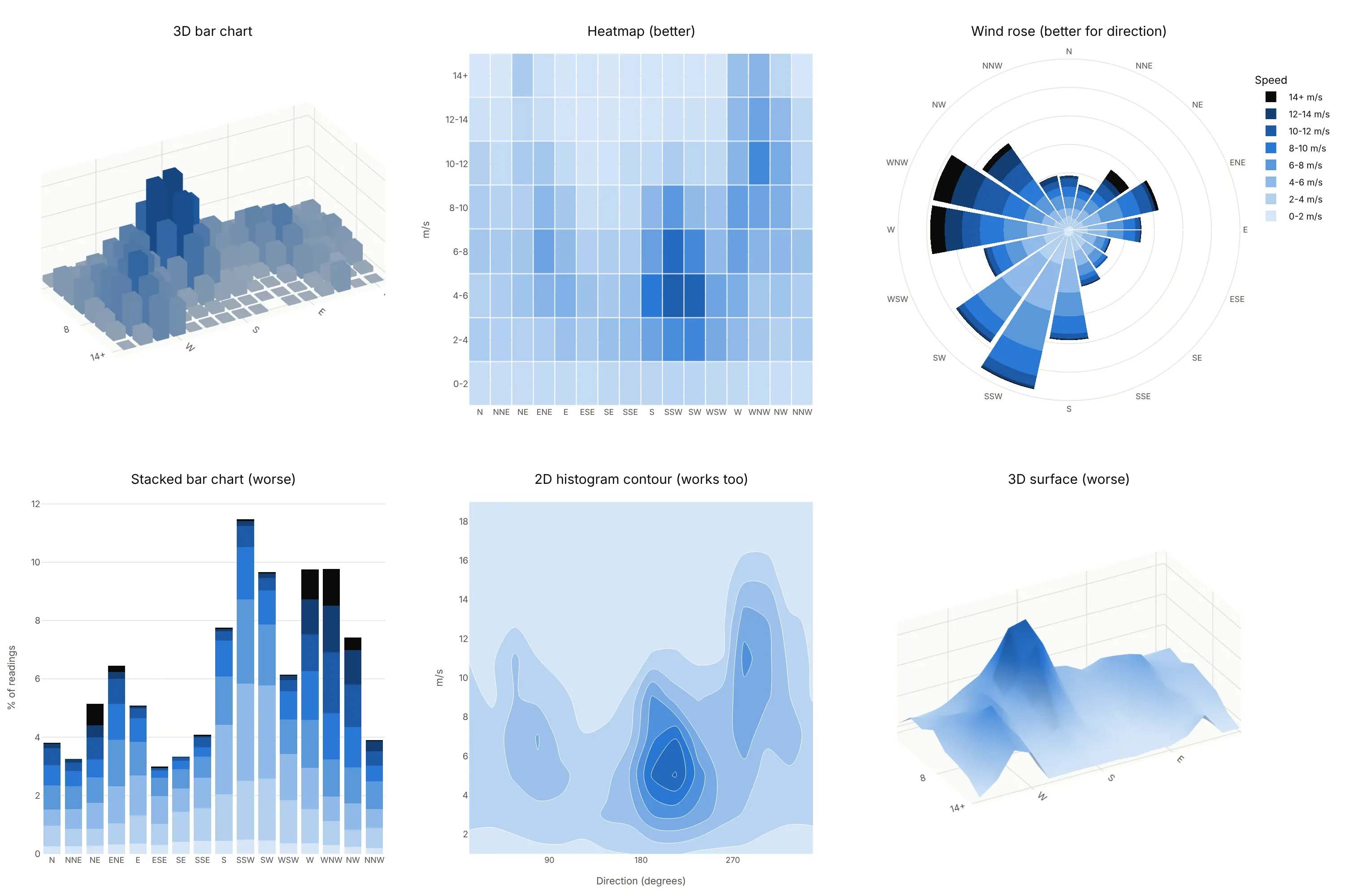
The buoy 44025 wind data drawn six ways: a 3D bar chart, a heatmap of direction against speed, a wind rose with stacked speed bands in each direction, a stacked bar chart by direction, a 2D histogram contour of direction in degrees against speed, and a 3D surface over the same grid

Heatmap (better for reading values). The same grid seen from straight above, with the value as color. Nothing hides, every cell can carry its number, and it prints well; you lose the sense of height.
Wind rose (better for direction). For directions, a circle is the natural axis: north is up and the two westerly regimes sit side by side instead of at opposite ends of a row.
Stacked bar chart (worse). It shows the total for each direction well, but only the bottom speed band starts from zero, so the bands above it are hard to compare.
2D histogram contour (works too). It smooths the counts into density contours, which shows the two peaks clearly and works for raw data without choosing bins in advance.
3D surface (worse for binned data). A surface joins neighboring cells with slopes, which suggests values between bins that don't exist. Use it for continuous data such as a yield curve or terrain.

The other good alternatives cut the grid into slices, so that each chart shows only two of the three variables. Call the share of readings A, the direction B and the speed C. Here are both versions on the same wind data:

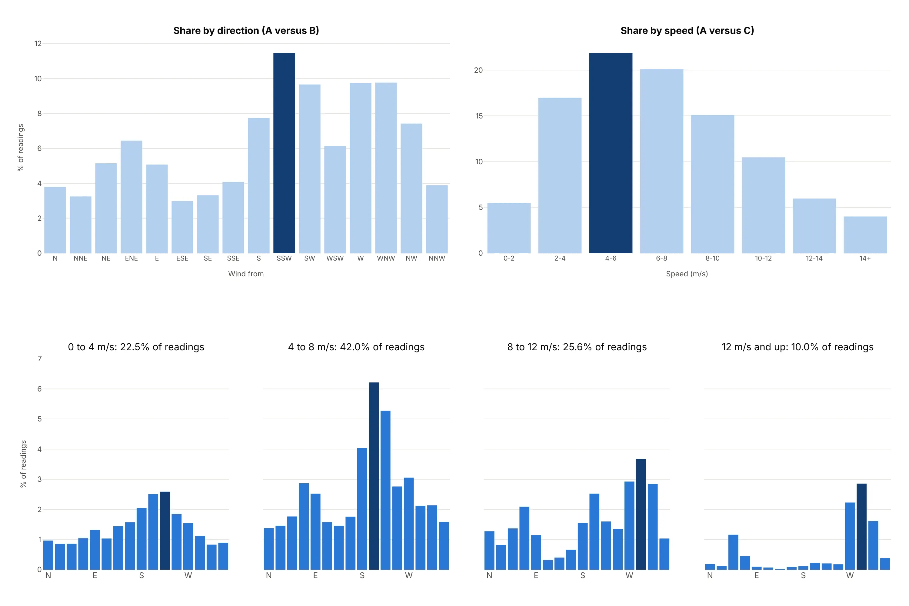
Wind data from buoy 44025 cut into slices: two bar charts side by side, share of readings by direction with south-southwest highest at 11.5% and share by speed with 4 to 6 m/s highest at 21.9%, and below them four small multiples of share by direction for the speed bands 0 to 4, 4 to 8, 8 to 12 and 12 m/s and up, on the same vertical scale, where south-southwest peaks at 6.2% in the 4 to 8 m/s panel and west-northwest peaks at 2.9% in the 12 m/s and up panel

Two 2D projections, A versus B and A versus C (works too). Add up the grid over one variable at a time: the share of readings by direction in one chart and by speed in the other. Each is an ordinary bar chart, so every value reads off one axis: south-southwest is the most common direction at 11.5% of readings, and 4 to 6 m/s is the most common speed band at 21.9%. Pick this pair when each variable answers its own question; what you lose is the link between them, because the speed chart can't tell you that most of the winds of 10 m/s or more (56%) come from the west, west-northwest and northwest. A versus B and B versus C works the same way with direction as the shared variable.
Small multiples of slices (better). One small bar chart of the share by direction for each speed band, all on the same vertical scale so the heights compare directly. The 4 to 8 m/s panel peaks at 6.2% of readings from the south-southwest, while the 12 m/s and up panel, which holds 10.0% of readings, peaks at 2.9% from the west-northwest, so the two wind regimes separate without any bar hiding another.

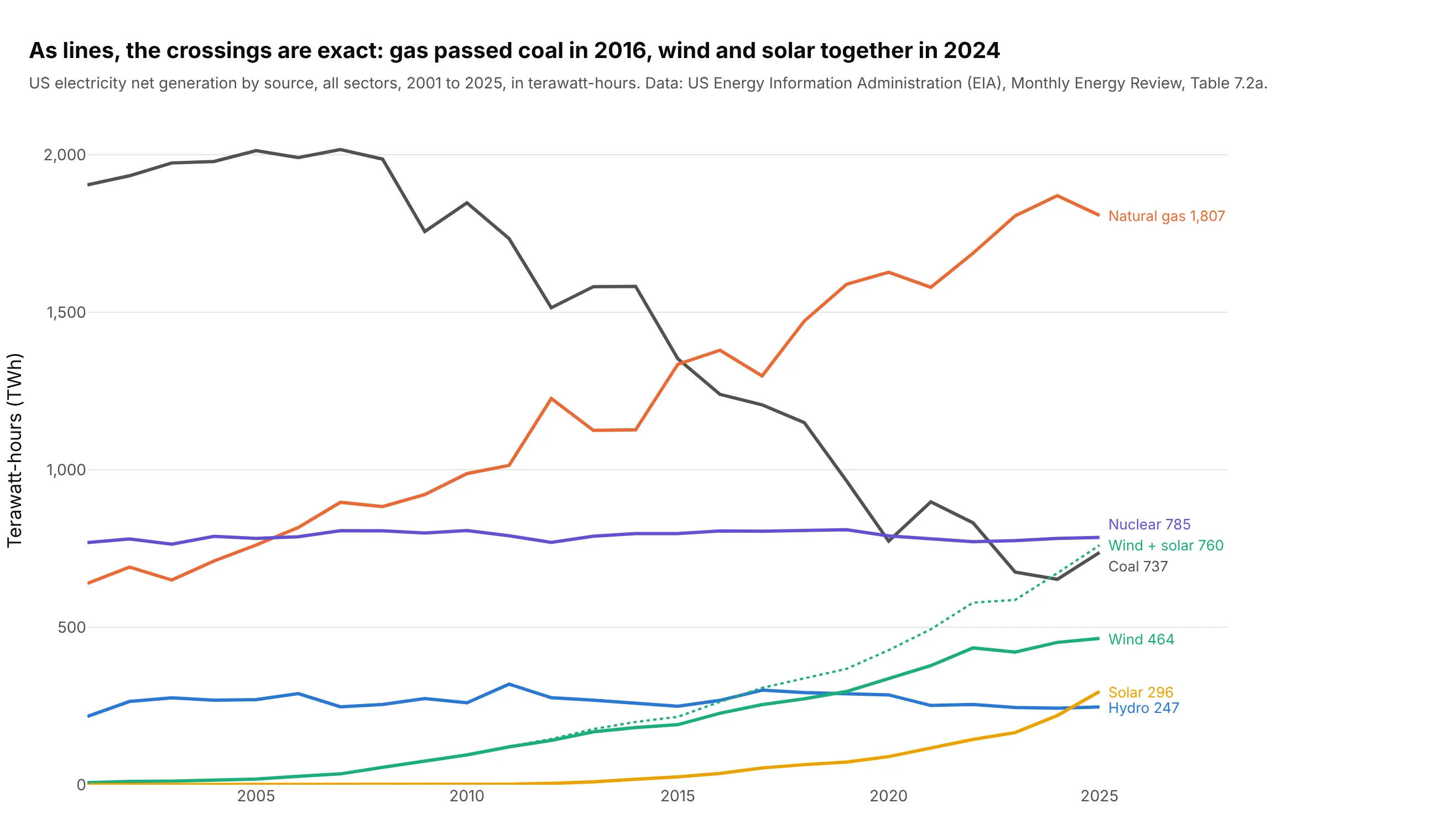
For a small table of categories over time, the case for 3D bars is weaker. Here's example 3's generation data as a line chart, where every value reads off one axis and the crossings are exact:

Line chart of US electricity generation by source from 2001 to 2025: natural gas crosses above coal in 2016, a dotted wind plus solar line crosses above coal in 2024, and the 2025 values are labeled: natural gas 1,807, nuclear 785, wind plus solar 760, coal 737, wind 464, solar 296 and hydro 247 terawatt-hours

How to make a 3D bar chart

With AI

ChatGPT, Claude Code, GitHub Copilot, Cursor and other AI tools are excellent at writing Plotly code. Name Plotly in the prompt, and say that the bars should be boxes in one go.Mesh3d trace, since there is no 3D bar trace to ask for by name:

Make a plotly 3D bar chart from wind.csv (columns: time, wdir in degrees, wspd in m/s).

- Count the readings with numpy.histogram2d in 16 direction sectors of 22.5 degrees (centered on N)
  and speed bins of 2 m/s, as a share of all readings.
- Draw each cell as a box in ONE go.Mesh3d trace: 8 corners and 12 triangles per bar, 0.8 wide so there is a gap between neighbors,
  colored by height with flatshading=True.
- Hover text per bar: "From SSW, 4-6 m/s: 3.33% of readings".
- Orthographic camera, looking from the high-speed side so short bars stand in front of tall ones.
- Axis titles "Wind from", "Speed (m/s)", "% of readings". A title that states the takeaway.

With Plotly Studio

Plotly Studio is a desktop app where you point an AI at a dataset and it builds charts and a Dash app around your questions. Ask for a 3D bar chart the same way:

Show monthly solar irradiance by hour of day as 3D bars (months on one axis, hours on the other), with an orthographic camera, a dropdown to pick the site, and a heatmap of the same grid next to it.

Make a 3D bar chart in Python or JavaScript

This is the code AI tools write under the hood. Plotly has no dedicated 3D bar trace, so you build the bars from go.Mesh3d: each bar is a box of 8 corners and 12 triangles, and putting every box into one trace keeps it fast. This helper does that for any grid:

import numpy as np
import pandas as pd
import plotly.graph_objects as go

def bars3d(x, y, z, width=0.8, depth=0.8, **kwargs):
    """One go.Mesh3d trace with a box (8 corners, 12 triangles) for every bar at (x, y) with height z."""
    x, y, z = (np.asarray(a, dtype=float).ravel() for a in (x, y, z))
    n, hw, hd = len(z), width / 2, depth / 2
    cx = np.stack([x - hw, x + hw, x + hw, x - hw] * 2, axis=1)  # corners 0-3 on the floor, 4-7 on top
    cy = np.stack([y - hd, y - hd, y + hd, y + hd] * 2, axis=1)
    cz = np.concatenate([np.zeros((n, 4)), np.repeat(z[:, None], 4, axis=1)], axis=1)
    faces = np.array([[0, 1, 2], [0, 2, 3], [4, 5, 6], [4, 6, 7], [0, 1, 5], [0, 5, 4],
                      [1, 2, 6], [1, 6, 5], [2, 3, 7], [2, 7, 6], [3, 0, 4], [3, 4, 7]])
    tri = (faces[None] + 8 * np.arange(n)[:, None, None]).reshape(-1, 3)
    return go.Mesh3d(x=cx.ravel(), y=cy.ravel(), z=cz.ravel(), i=tri[:, 0], j=tri[:, 1], k=tri[:, 2],
                     intensity=cz.ravel(), flatshading=True, **kwargs)

# A 2D histogram of wind direction (16 sectors) and speed (2 m/s bins)
df = pd.read_csv("wind.csv")  # columns: time, wdir (degrees), wspd (m/s), gst
counts, _, _ = np.histogram2d(df.wspd, (df.wdir + 11.25) % 360, bins=[np.arange(0, 22, 2), np.arange(0, 361, 22.5)])
share = counts / counts.sum() * 100
speed, sector = np.meshgrid(np.arange(share.shape[0]), np.arange(share.shape[1]), indexing="ij")

fig = go.Figure(bars3d(sector, speed, share, colorscale="Blues"))
fig.update_layout(scene=dict(
    xaxis=dict(title="Wind from", tickvals=[0, 4, 8, 12], ticktext=["N", "E", "S", "W"]),
    yaxis=dict(title="Speed (m/s)", tickvals=list(range(10)), ticktext=[str(v) for v in range(0, 20, 2)]),
    zaxis=dict(title="% of readings"),
    camera=dict(projection=dict(type="orthographic")),
))
fig.show()

intensity colors each bar by its height; pass color="#2a78d6" instead for one color, or facecolor with one color per triangle (12 per bar) to color bars by category, as in the generation chart. For bars that go below zero, like the stock returns in example 4 below, use the value as the top and 0 as the bottom; the triangles work either way. The guide's full helper, with hover text and category colors, is bar3d.py in the code folder for this post.

If you're coming from matplotlib, Axes3D.bar3d(x, y, z, dx, dy, dz) takes the same inputs (a position, a base and a size for each bar) and draws a static image; with Plotly the chart rotates, zooms and shows a hover label for every bar. MATLAB's bar3(Z) corresponds to calling the helper on the rows and columns of Z.

In JavaScript, plotly.js draws the same boxes from a mesh3d trace:

<div id="chart"></div>
<script src="https://cdn.plot.ly/plotly-4.1.1.min.js"></script>
<script>
  // Cars per 500 lb weight bin (rows, 1,500 to 5,500 lb) and 5 mpg bin (columns, 10 to 45 mpg), UCI Auto MPG
  const counts = [
    [0, 0, 0, 11, 16, 13, 3],  [0, 3, 19, 34, 30, 11, 5], [0, 11, 35, 28, 8, 2, 0], [2, 31, 21, 2, 2, 1, 0],
    [8, 32, 3, 2, 0, 0, 0],    [27, 20, 0, 0, 0, 0, 0],   [14, 1, 0, 0, 0, 0, 0],   [1, 0, 0, 0, 0, 0, 0]];
  const faces = [[0,1,2],[0,2,3],[4,5,6],[4,6,7],[0,1,5],[0,5,4],[1,2,6],[1,6,5],[2,3,7],[2,7,6],[3,0,4],[3,4,7]];
  const x = [], y = [], z = [], i = [], j = [], k = [];
  counts.forEach((row, r) => row.forEach((h, c) => {
    if (h === 0) return;
    const n = x.length;  // index of this bar's first corner
    const xs = [c - 0.4, c + 0.4, c + 0.4, c - 0.4], ys = [r - 0.4, r - 0.4, r + 0.4, r + 0.4];
    for (let v = 0; v < 8; v++) { x.push(xs[v % 4]); y.push(ys[v % 4]); z.push(v < 4 ? 0 : h); }
    faces.forEach(f => { i.push(n + f[0]); j.push(n + f[1]); k.push(n + f[2]); });
  }));

  Plotly.newPlot("chart", [{type: "mesh3d", x, y, z, i, j, k, intensity: z, colorscale: "Blues", flatshading: true}], {
    width: 800, height: 600,
    scene: {
      xaxis: {title: {text: "Miles per gallon"}, tickvals: [0, 2, 4, 6], ticktext: ["10", "20", "30", "40"]},
      yaxis: {title: {text: "Weight (lb)"}, tickvals: [0, 2, 4, 6], ticktext: ["1,500", "2,500", "3,500", "4,500"]},
      zaxis: {title: {text: "Cars"}},
      camera: {projection: {type: "orthographic"}}
    }
  });
</script>

In Excel, a 3-D column chart comes from Insert, Charts, Column, 3-D Column, and works on a small table; for a 2D histogram you count the cells first (with COUNTIFS), and you can't hover, rotate freely or draw thousands of bars.

Share it

Every Plotly chart has a Share chart button (the cloud icon in its toolbar) that uploads it to Plotly Cloud and gives you a link. Only you can see it until you change its visibility.

For a live app, put the chart in a Dash app and publish it with the Plotly Cloud command-line interface (CLI). Coding agents can run these commands for you:

pip install "dash[cloud]"
plotly user login
plotly app publish

If your data has to stay in your own cloud or data center, publish to Dash Enterprise instead.

Dos and don'ts

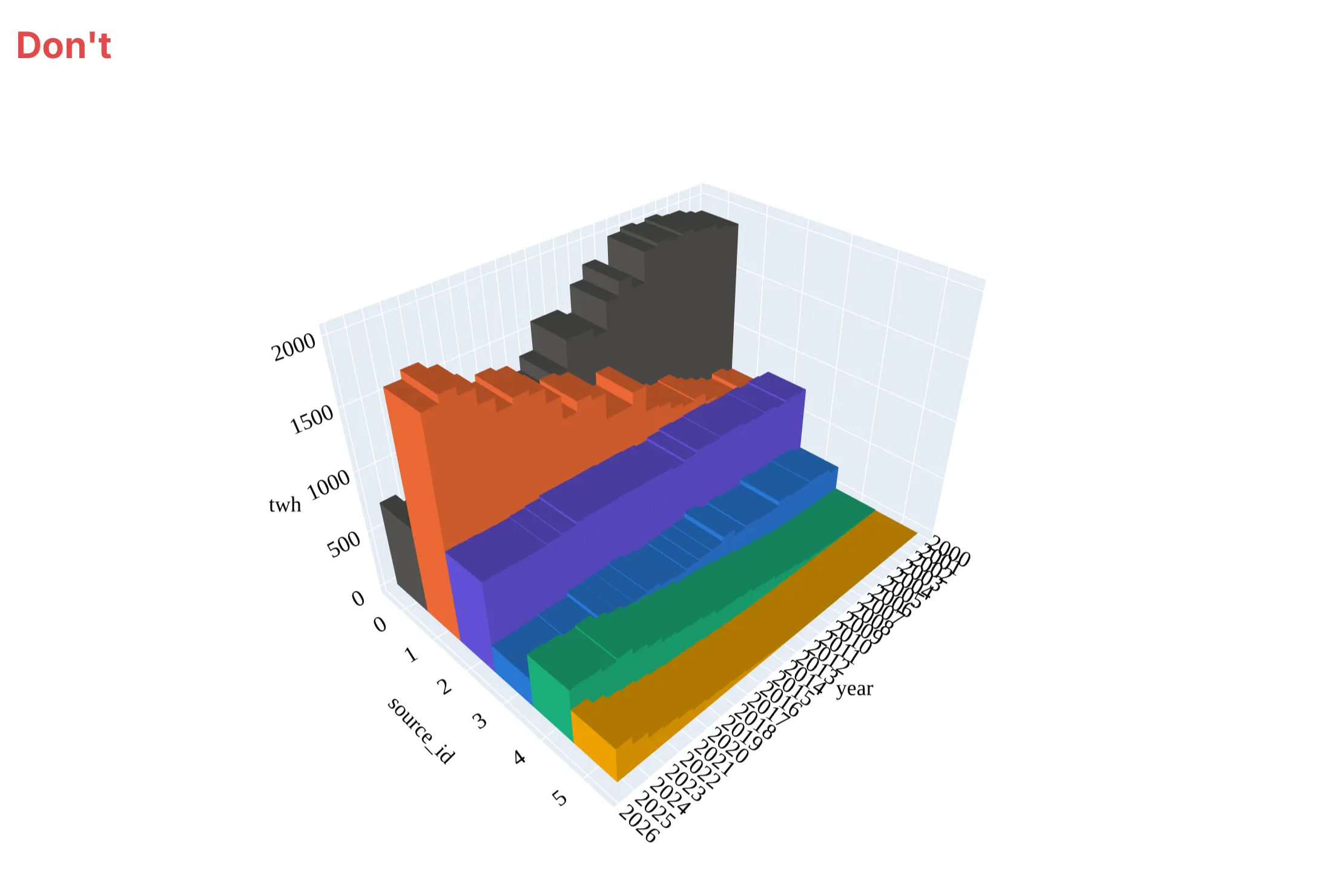
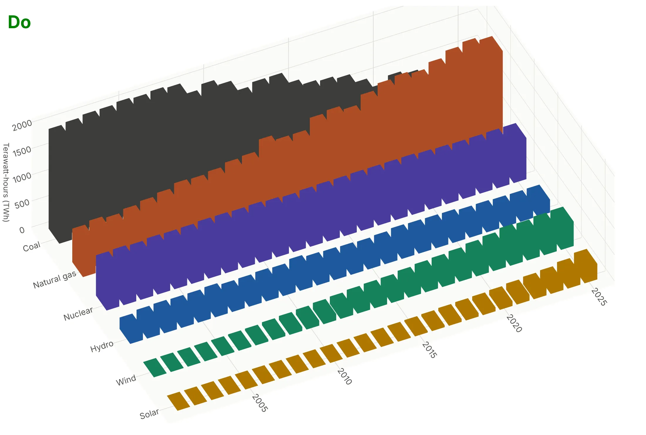
Most of what goes wrong with a 3D bar chart is about what hides what, so the fixes are about order, spacing and the camera. Here is the US generation data both ways, in the same colors.

Don't put the tallest rows (coal and gas) in front where they cover everything behind them, let the bars touch with no gaps, keep the default perspective camera at its default angle, leave raw column names (year, source_id, twh) as axis titles with a tick for every year, or use a default serif font:

The US generation data as 3D bars with coal and natural gas in the front rows hiding nuclear, hydro, wind and solar behind them, bars touching with no gaps, axis titles year, source_id and twh, overlapping year ticks and a serif font

Do order the rows from the smallest in front to the largest at the back, leave gaps between bars, space the rows apart, use an orthographic camera raised enough to see over the front rows, name the rows in words and put the unit on the height axis. Even this better 3D version hides part of coal behind natural gas after 2016, which is why the line chart in the Alternatives section shows the crossover better:

The same data with solar, wind, hydro, nuclear, natural gas and coal rows from front to back, gaps between bars, wider gaps between the rows, an orthographic camera at a three-quarter angle, the sources named and an axis titled Terawatt-hours (TWh), every fifth year labeled

Checklist

Put all the bars in one go.Mesh3d trace; one trace per bar is many times slower.
Use an orthographic camera so equal values look equal.
Order rows so short bars stand in front of tall ones, and choose the camera angle from the data.
Leave gaps between bars (a width of 0.75 to 0.85) because bars of similar color blend together when they touch. Outline lines drawn as a go.Scatter3d trace showed through the neighboring bars as dashes in our renders, so we left them out and let the shading and the gaps separate the bars.
Add hover text with the exact value of each bar, since heights are hard to read in 3D.
Show a heatmap of the same grid when the exact values matter.

Don't

Use 3D bars for one row of values; a flat bar chart says the same thing more clearly.
Draw a 3D surface over binned counts; it invents values between the bins.
Publish a static image from an angle where tall bars hide the ones you talk about in the text.

Options to customize

A 3D bar chart in Plotly is a mesh3d trace of boxes inside a 3D scene, so these are the options that matter most. The full lists are in the mesh3d trace reference and the 3D scene layout reference.

x, y, z and i, j, k: the corners of every box and the three corner indices of every triangle (8 corners and 12 triangles per bar).
intensity, colorscale, cmin, cmax: color each bar by its height (or any value) on a color scale; set cmin and cmax so several charts share one scale.
color or facecolor: one color for every bar, or one color per triangle to color bars by category.
flatshading=True and lighting (ambient, diffuse, specular): flat faces with distinct shading make each side of a box readable; more ambient keeps the colors close to the color scale.
hovertext with hoverinfo="text": one label per corner (repeat each bar's label 8 times) so hovering a bar shows its exact value.
scene.camera.projection.type="orthographic": draws every bar at the same scale; the default is "perspective".
scene.camera.eye and center: where the camera stands and what it looks at; move it so short bars are in front of tall ones.
scene.aspectmode="manual" with aspectratio: the box proportions, such as a long axis for years and a low height.
scene.xaxis.tickvals and ticktext: category names on the floor axes, since the bars sit at numeric positions 0, 1, 2 and so on.
scene.annotations: text labels with arrows pinned to a point in 3D, such as the tallest bar.
go.Scatter3d(mode="lines") with None between segments: a map outline on the floor, as in example 2 below. Avoid using it for bar edges, which can show through neighboring bars.
numpy.histogram2d (or pandas.crosstab): counts the raw data into the grid of bars for a 3D histogram.

More 3D bar chart examples

Six more 3D bar charts built from real public data, each with its source, the technique that makes it work and a prompt to rebuild it.

1. Sunlight by month and hour of day in the Mojave Desert

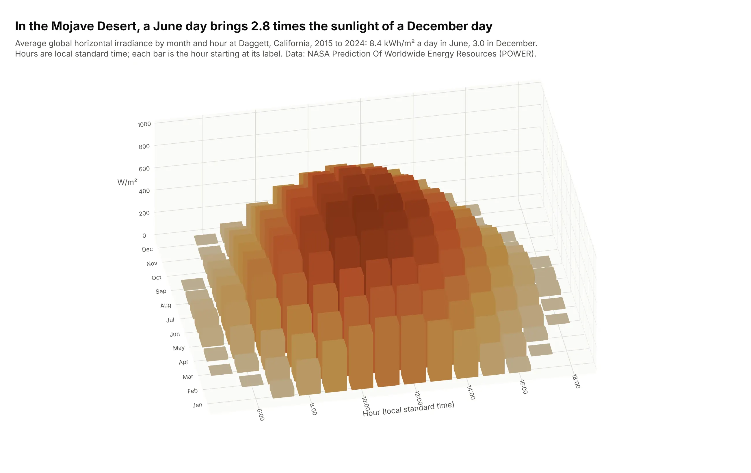
3D bar chart of average global horizontal irradiance at Daggett, California, from 2015 to 2024, by month and hour from 5:00 to 19:00: the bars form a hill that is tallest and widest in June, peaking near 1,000 W/m² at 11:00, and low and narrow in December

A June day at Daggett, California, brings 8.4 kWh/m² of sunlight and a December day 3.0, 2.8 times less, because the December sun is both lower (503 W/m² at its best hour against 995 in June) and up for fewer hours. Solar engineers read this month-by-hour grid to size panels and storage. Data: NASA Prediction Of Worldwide Energy Resources (POWER), hourly all-sky irradiance, 2015 to 2024.

Tip: leave out the night hours, which are all zero and only push the daytime bars together.

Get the data from the NASA POWER hourly API (community RE, parameter ALLSKY_SFC_SW_DWN, global horizontal
irradiance in W/m2, time-standard LST) for latitude 34.86, longitude -116.78 (Daggett, California),
2015-2024 (columns: time, ghi).

Build a plotly 3D bar chart of the mean ghi by month (12 rows) and hour of day (5:00 to 19:00), boxes
in one go.Mesh3d trace colored by height on an orange scale, an orthographic camera, and the June and
December daily totals in kWh/m2 in the subtitle.

2. US wind power capacity on a map grid

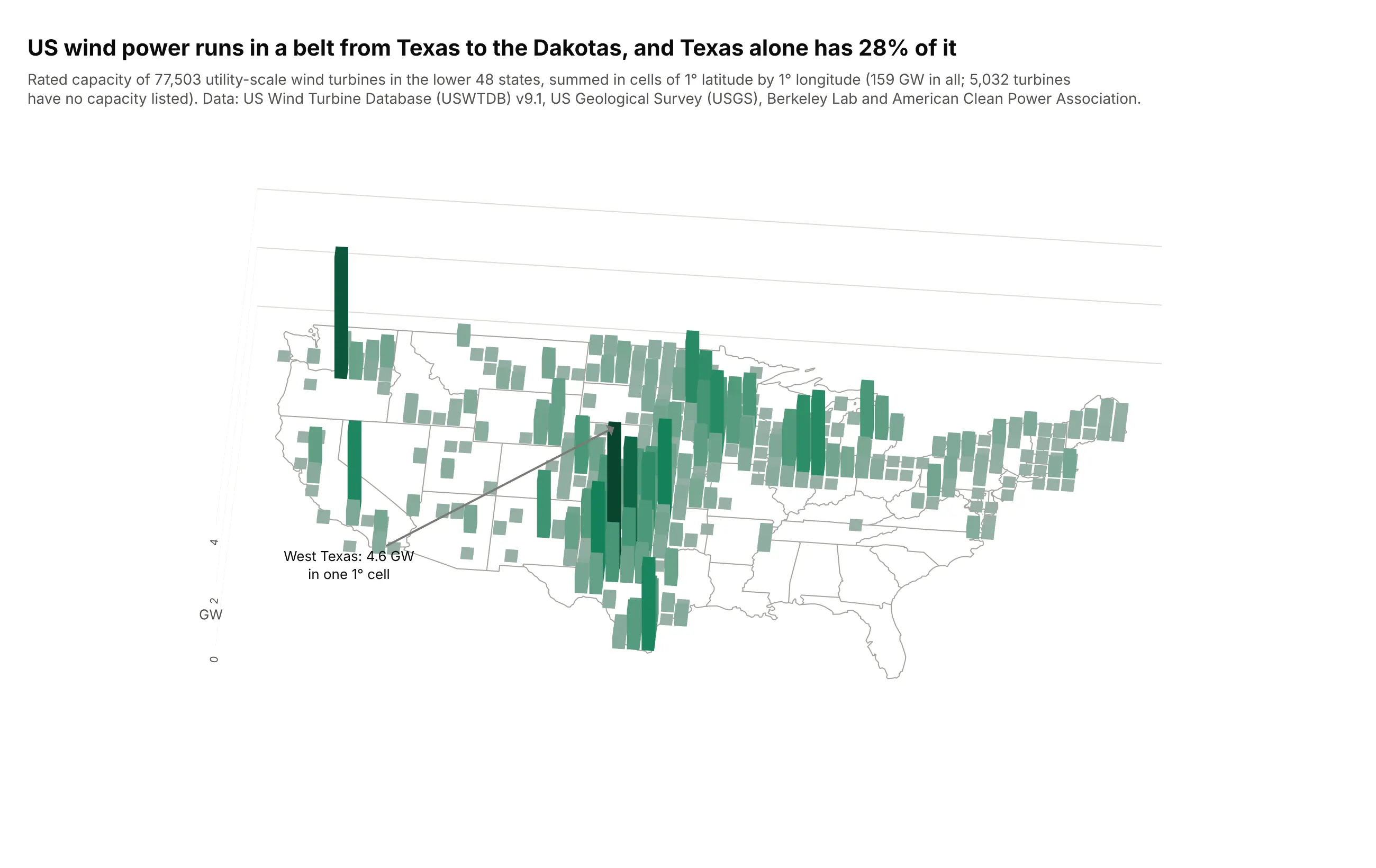
3D bars standing on an outline map of the lower 48 US states, one bar for each 1-degree cell of latitude and longitude with height equal to its wind turbine capacity: tall bars run from Texas north through Oklahoma, Kansas and Iowa to the Dakotas, with the tallest, 4.6 GW, in West Texas and another tall one on the Columbia River

Summing 77,503 turbines (159 GW) into 1-degree cells shows a belt of wind power from Texas to the Dakotas; Texas alone has 28% of the capacity and one West Texas cell holds 4.6 GW. 5,032 turbines in the database have no capacity listed. Data: US Wind Turbine Database (USWTDB) v9.1, US Geological Survey (USGS), Berkeley Lab and the American Clean Power Association.

Tip: draw the state outlines as a go.Scatter3d line at z = 0 and set the aspect ratio from the map's width and height, so the bars stand on a recognizable map.

Get the data from the US Wind Turbine Database (USWTDB, US Geological Survey, Berkeley Lab and
the American Clean Power Association) CSV, lower 48 states (columns: case_id, t_state, p_name, p_year,
t_cap in kW, xlong, ylat), and US state outlines as GeoJSON.

Build a plotly 3D bar chart on a map: sum t_cap into 1-degree latitude x longitude cells, one box per
cell in a go.Mesh3d trace colored by GW, state outlines as a go.Scatter3d line at z = 0, an
orthographic camera from the south, and the largest cell labeled.

3. Clinical trials by phase and start year

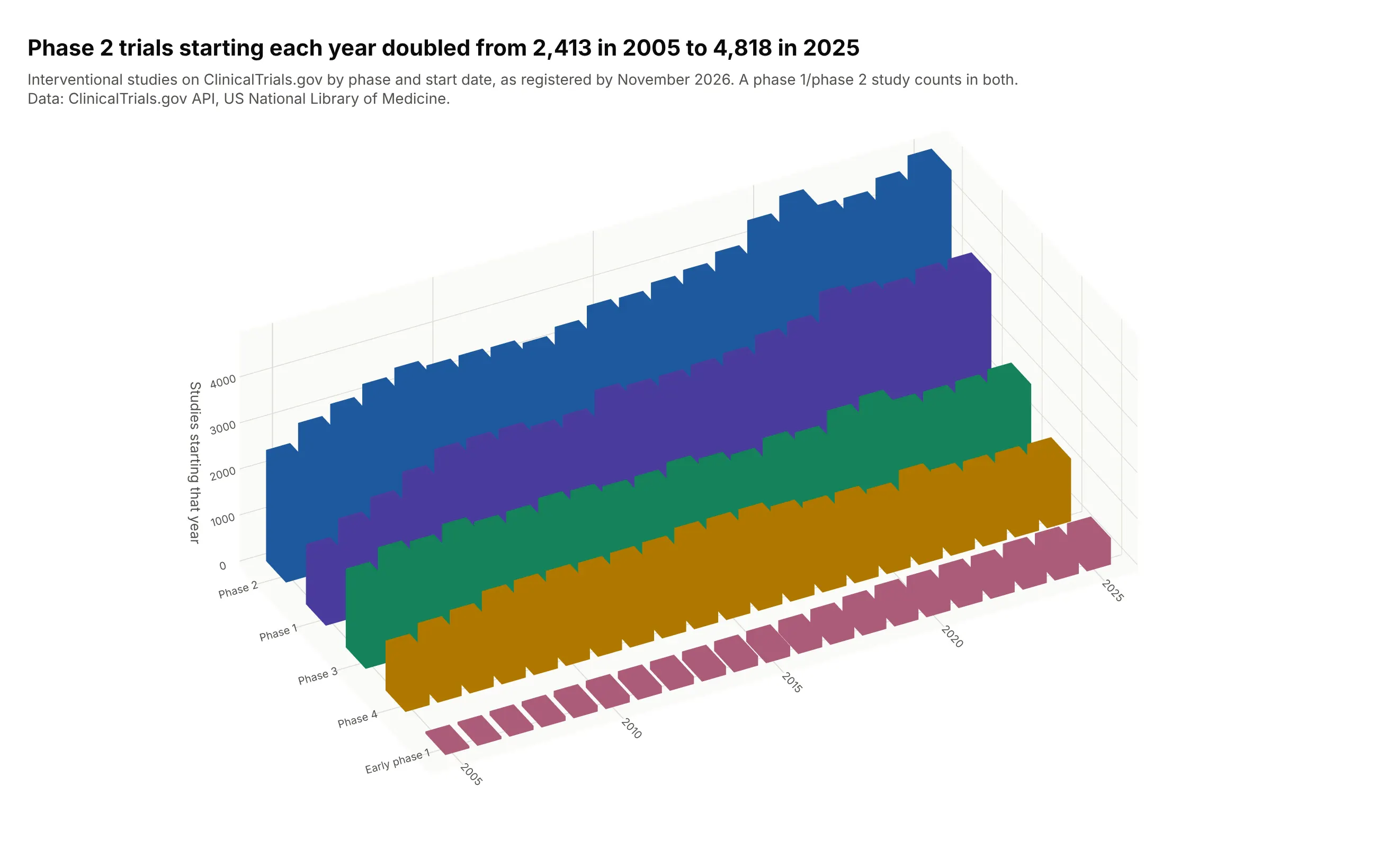
3-D column chart of interventional studies on ClinicalTrials.gov by phase and start year from 2005 to 2025, rows from front to back for early phase 1, phase 4, phase 3, phase 1 and phase 2: the phase 2 row at the back rises from 2,413 to 4,818 studies a year

Phase 2 trials starting each year doubled, from 2,413 in 2005 to 4,818 in 2025, while phase 4 rose to 1,738 in 2016 and fell back to 1,362. Ordering the rows from the smallest at the front to the largest at the back keeps every bar visible. Data: ClinicalTrials.gov API, US National Library of Medicine, retrieved November 2026.

Tip: sort the rows by size before you draw them; with five rows in the right order, nothing hides.

Get the data from the ClinicalTrials.gov API v2 (US National Library of Medicine): the count of interventional
studies for each phase (early phase 1, phase 1 to phase 4) and each start year 2005-2025, using
countTotal with filter.advanced (columns: phase, year, studies).

Build a plotly 3D column chart: years along the front, phases going back from smallest to largest,
one color per phase, boxes in one go.Mesh3d trace, an orthographic camera.

4. Monthly stock market returns, with bars below zero

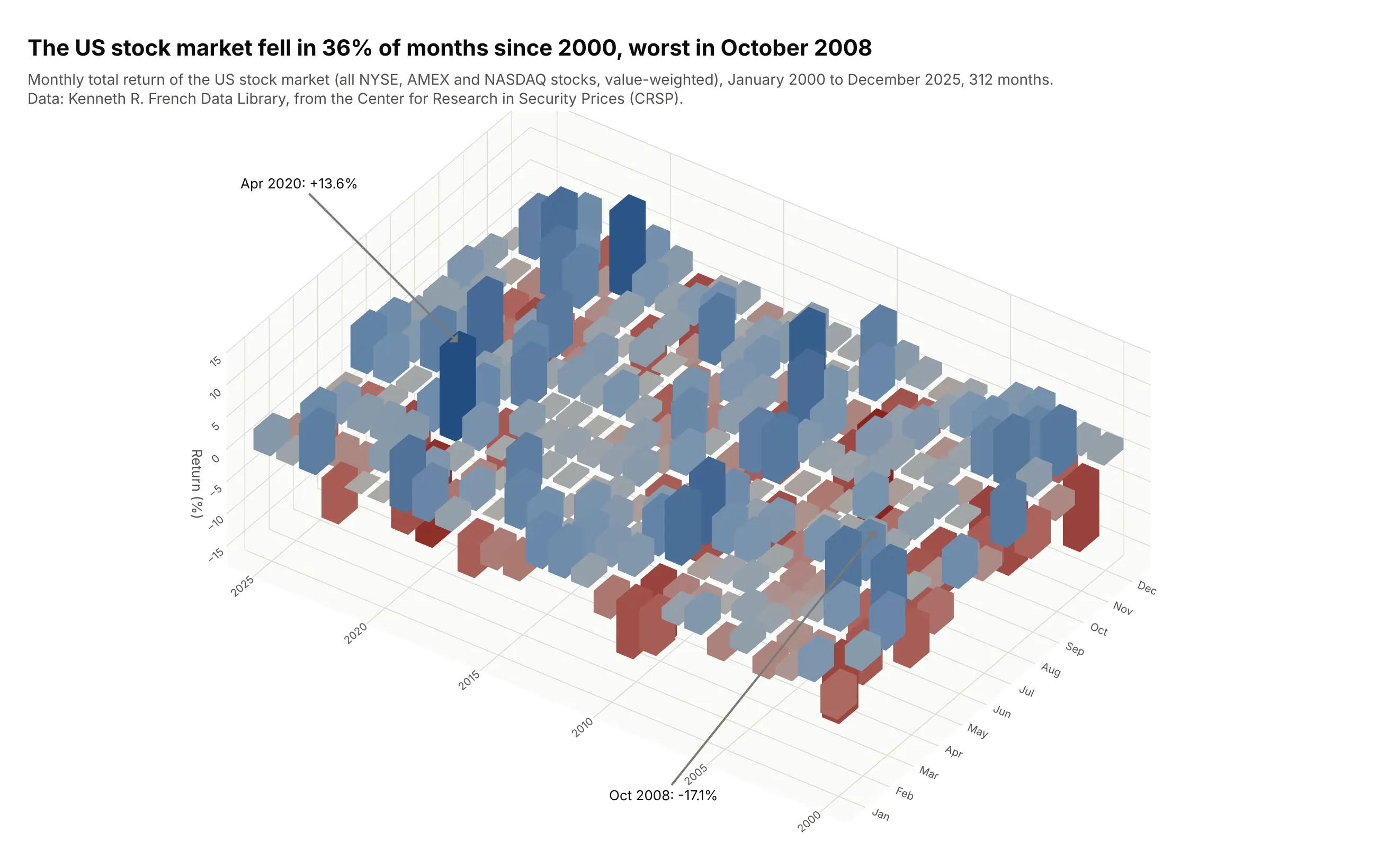
3D bar chart of 312 monthly returns of the US stock market from January 2000 to December 2025, years along one axis and months along the other, blue bars rising for gains and red bars dropping below the floor for losses, with October 2008 at -17.1% and April 2020 at +13.6% labeled

The US stock market fell in 36% of the 312 months from 2000 to 2025, worst in October 2008 (-17.1%) and best in April 2020 (+13.6%). Bars that drop below the floor make the crashes visible as pits, but with 312 bars many of them hide each other. Data: Kenneth R. French Data Library, Fama/French 3 Factors (market return from the Center for Research in Security Prices, CRSP).

Tip: for values that go negative, use a diverging color scale centered on zero so a bar's color says its sign even when its top is hidden.

Get the data from the Kenneth R. French Data Library: Fama/French 3 Factors [Monthly], with the market
return = Mkt-RF + RF in percent, January 2000 to December 2025 (columns: year, month, ret).

Build a plotly 3D bar chart of ret by year and month, boxes in one go.Mesh3d trace from 0 to ret
(down for losses), a red-gray-blue color scale centered on zero, the best and worst months labeled.

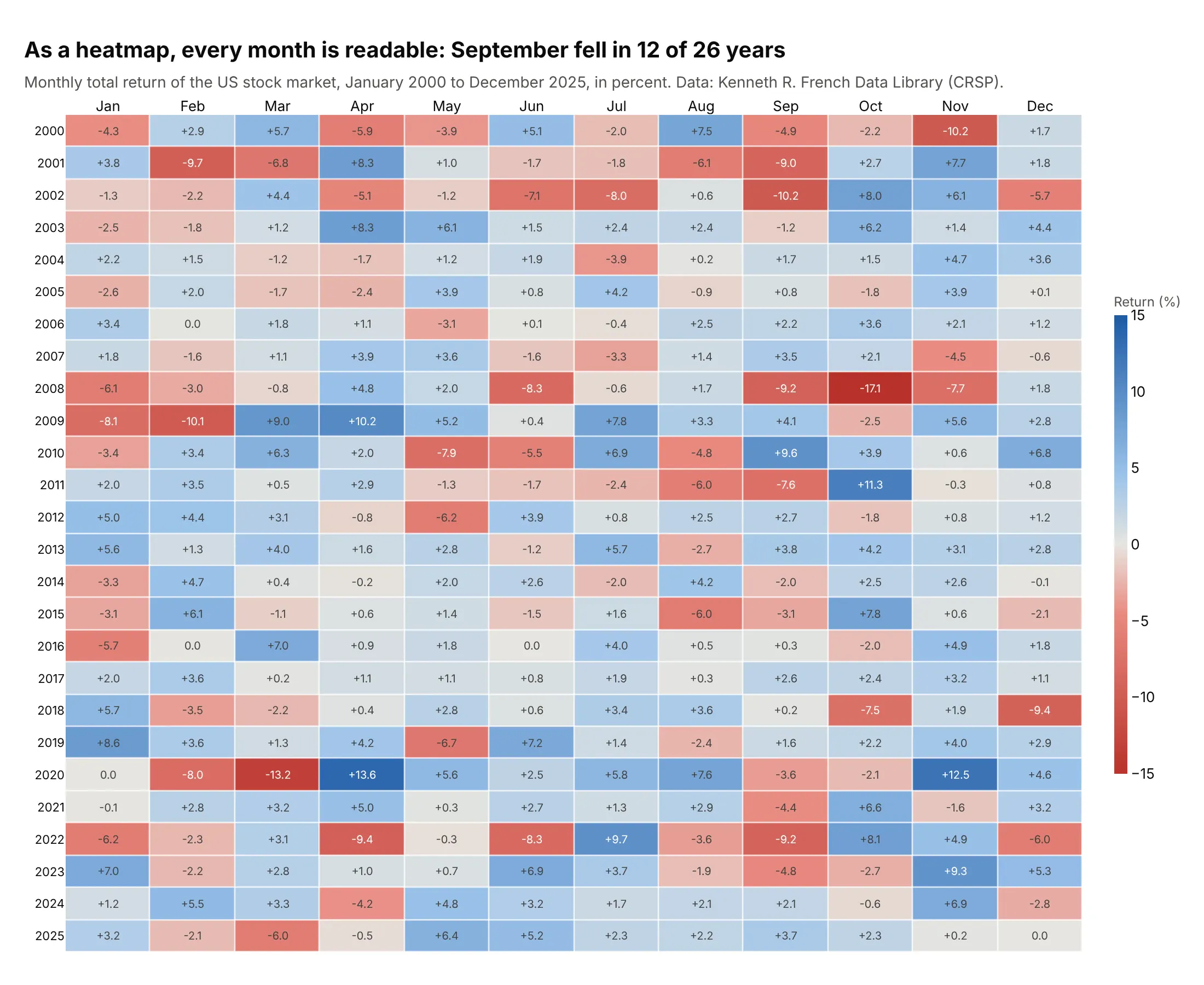
Another way to see it: the same returns as a heatmap, where every month is visible and printed, and the pattern of Septembers (12 of 26 negative) is easy to find:

Heatmap of the same 312 monthly returns with years down and months across, each cell printed with its return and colored red for losses and blue for gains, October 2008 at -17.1 the darkest red

5. A Hertzsprung-Russell diagram as a 3D histogram

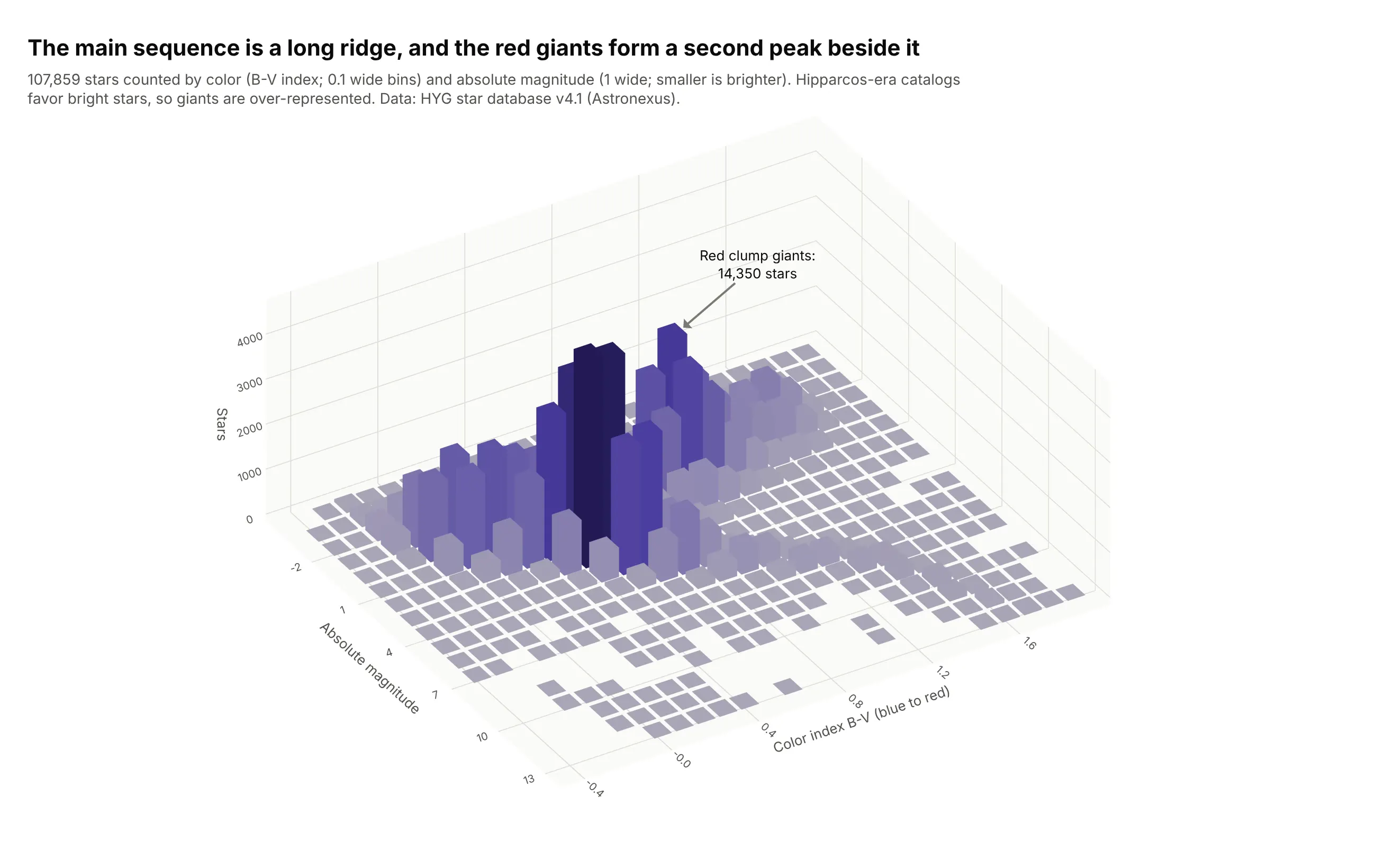
3D histogram of 107,859 stars counted by color index B-V and absolute magnitude: a long ridge of main sequence stars rises to 4,631 stars at B-V 0.4 to 0.5 and magnitude 3 to 4, and a separate peak of red clump giants at B-V near 1.0 and magnitude 0 to 1 holds 14,350 stars in its region

The Hertzsprung-Russell (H-R) diagram plots a star's color against its brightness; drawn as a scatter plot of 107,859 stars, its dense parts turn into a solid blob. As a 3D histogram the main sequence becomes a ridge and the red clump, 14,350 helium-burning giants, a second peak. Data: HYG star database v4.1 (Hipparcos, Yale Bright Star and Gliese catalogs).

Tip: keep the axis directions of the field's usual chart (bright stars at the back, like the top of an H-R diagram), so astronomers recognize it.

Get the data from the HYG star database v4.1 (Astronexus GitHub, hyg/CURRENT/hygdata_v41.csv, combining
the Hipparcos, Yale Bright Star and Gliese catalogs), stars with a color index and a known distance (columns: ci, absmag, dist).

Build a plotly 3D histogram: numpy.histogram2d of absmag (1 wide, -4 to 14) and ci (0.1 wide, -0.4 to
2.0), boxes in one go.Mesh3d trace colored by count, bright stars at the back, the red clump labeled.

6. A rainflow matrix of temperature cycles

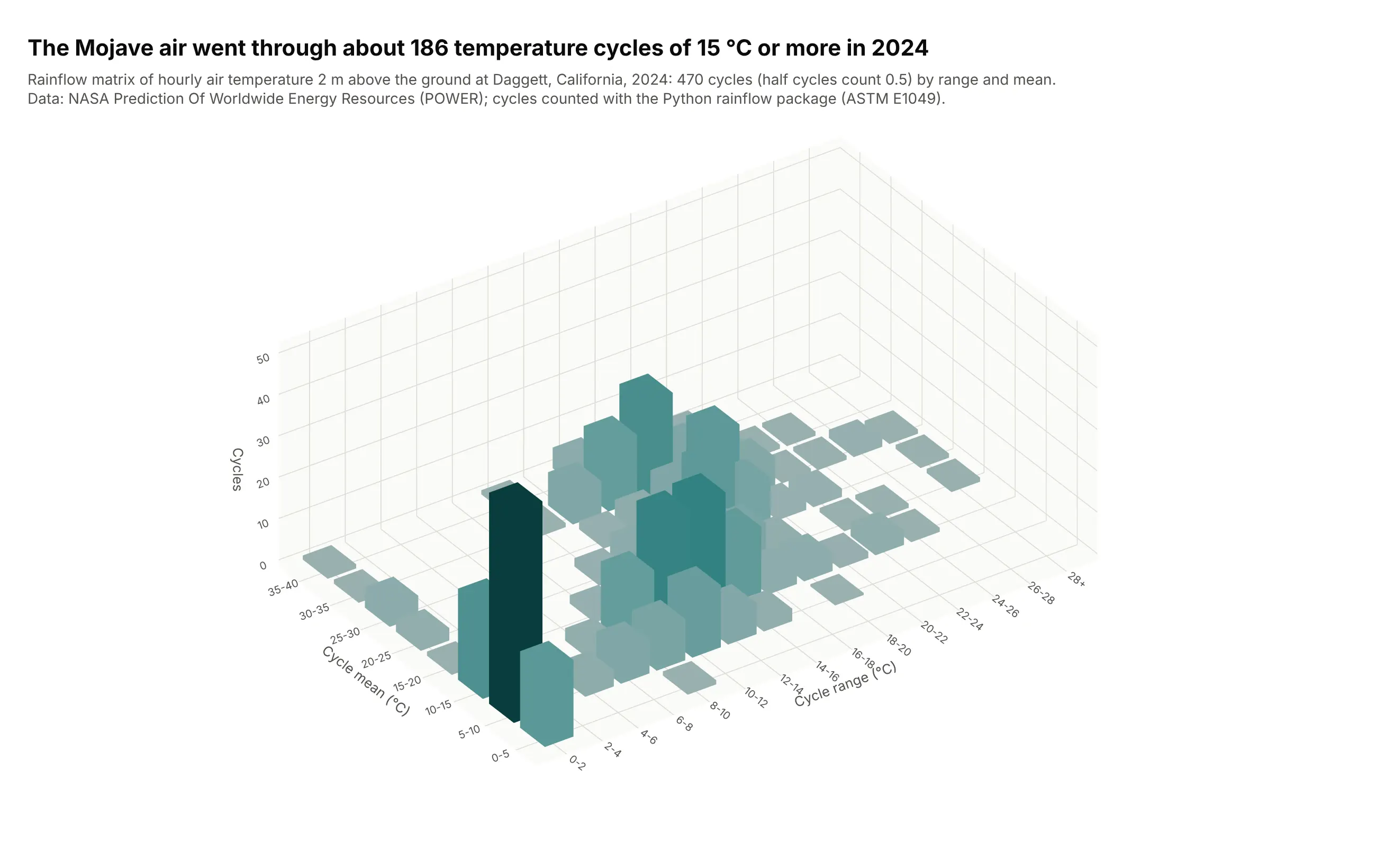
Rainflow matrix of hourly air temperature at Daggett, California, in 2024 as 3D bars of cycle counts by cycle range in 2 °C bins and cycle mean in 5 °C bins: most cycles have ranges under 10 °C, and a group of daily cycles with ranges of 15 to 25 °C stands out, 185.5 cycles of 15 °C or more in all

Rainflow counting (ASTM E1049) turns a load history into cycles of a given range and mean, and fatigue engineers draw the counts as 3D bars. A year of air temperature in the Mojave holds 185.5 cycles of 15 °C or more, the daily swings that fatigue solder joints in outdoor electronics. Data: NASA POWER hourly temperature at 2 m, Daggett, California, 2024; cycles from the Python rainflow package.

Tip: count half cycles as 0.5, as the standard does, and say so on the chart.

Get the data from the NASA POWER hourly API (parameter T2M, air temperature at 2 m in °C, time-standard LST)
for latitude 34.86, longitude -116.78 (Daggett, California), 2024 (columns: time, t2m).

Count cycles with rainflow.extract_cycles(t2m) and build a plotly 3D bar chart (rainflow matrix) of
the cycle counts by range (2 °C bins) and mean (5 °C bins), boxes in one go.Mesh3d trace, orthographic camera.