Gantt Charts - A Complete Guide

TL;DR

• A Gantt chart draws each task, phase or event as a horizontal bar from its start date to its end date, one row per task, on a shared time axis, so you can see when things happen, how long they take and what overlaps.
• Use one for project plans, clinical trial programs, support windows, asset lifetimes and anything else where every item has a start and an end.
• Use a sorted bar chart instead when only the durations matter, and a dot plot when each item has a single date.
• Any coding agent can make one with Plotly in a minute. In Python it's px.timeline(df, x_start=..., x_end=..., y=...).

What is a Gantt chart?

Gantt charts look like this:

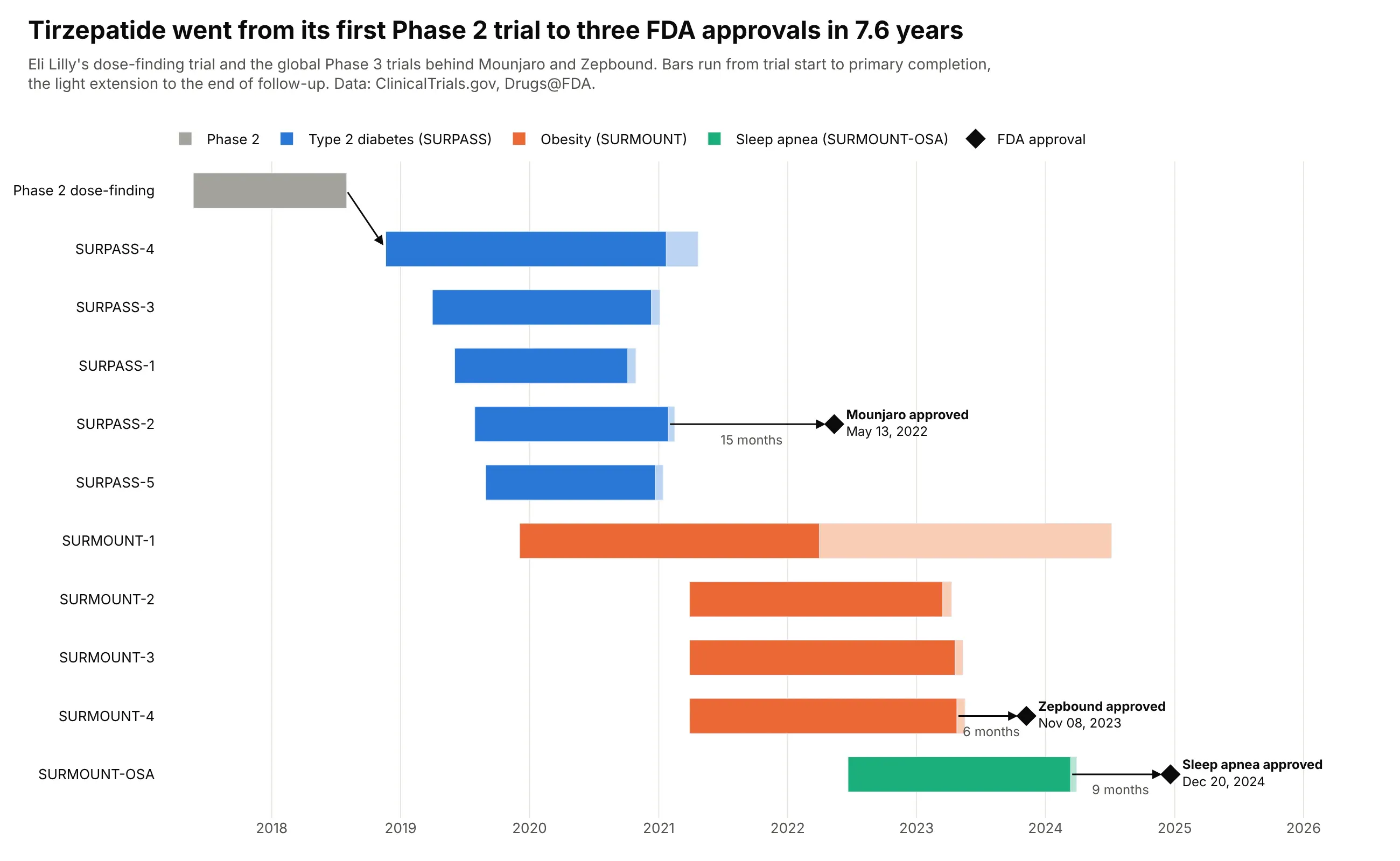
Data: ClinicalTrials.gov, Drugs@FDA.

How do you read a Gantt chart? In the example above, notice these things:

• Each row is one of tirzepatide's trials, and its bar runs from the day the trial started to its primary completion, with a lighter extension to the end of follow-up.
• The rows are grouped by program and sorted by start date within each group, and each program has its own color, so the blue SURPASS diabetes trials, which mostly ran at the same time, read as one block.
• The black diamonds are FDA approvals, which happen on a single day, so they are drawn as points with their dates next to them instead of as bars.
• The arrows show what came after what: the first Phase 3 trial started after the Phase 2 trial ended, and each approval came after the last readout of its program, with Mounjaro approved 15 months after the SURPASS-2 readout.
• SURMOUNT-1's long pale tail is follow-up that ran into 2024, after Zepbound was already approved, so an approval can come before every bar in its program has ended.

It's often used for charts like these:

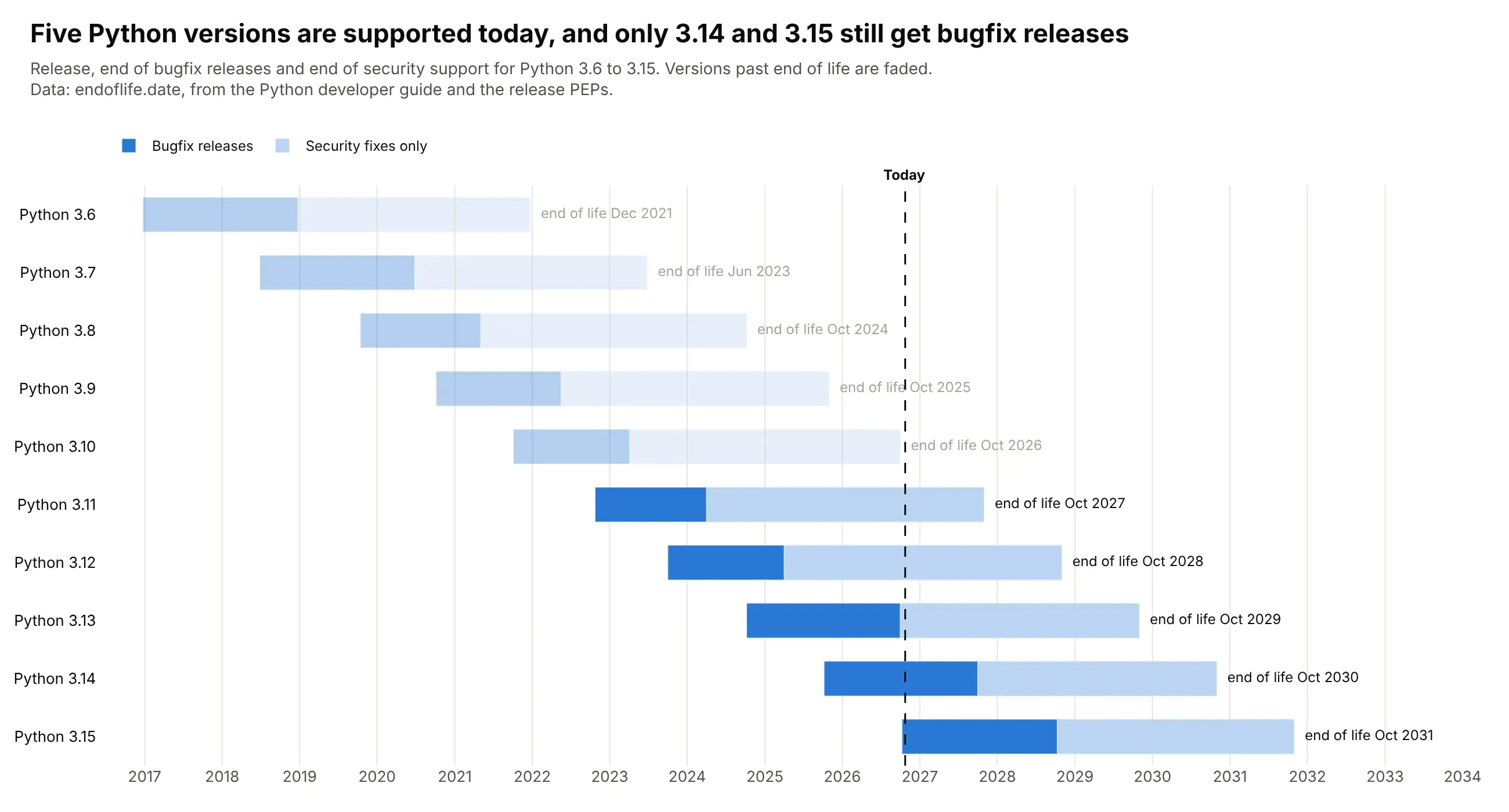
Support windows. Five Python versions are supported today, only 3.14 and 3.15 still get bugfix releases, and every version since 3.8 gets about five years before end of life. Data: endoflife.date, from the Python developer guide.

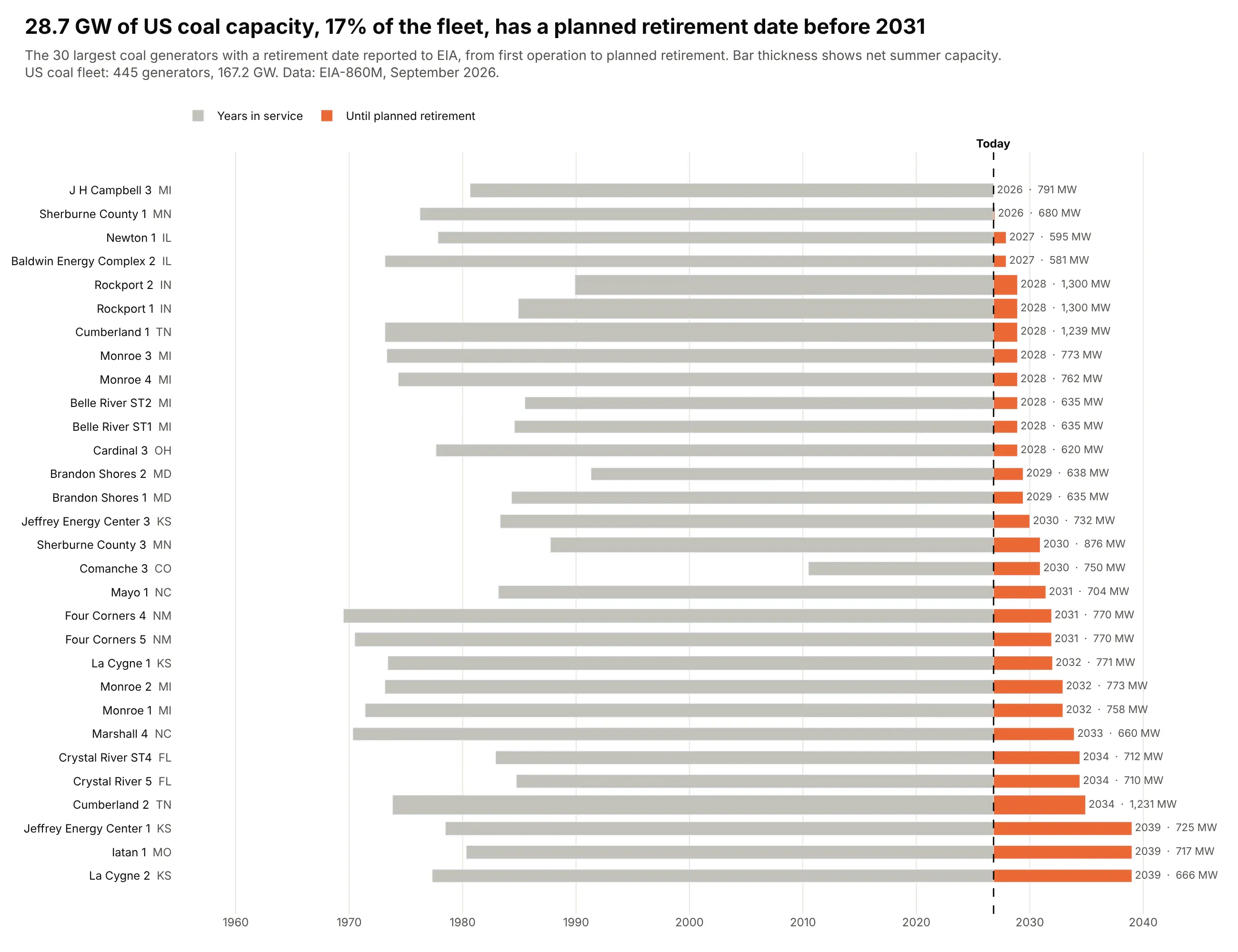
Asset lifetimes. Owners have told EIA that 28.7 GW of US coal capacity, 17% of the 167.2 GW still running, will retire before 2031, and the 30 largest of those units have run for a median of 48 years. Data: EIA-860M, September 2026.

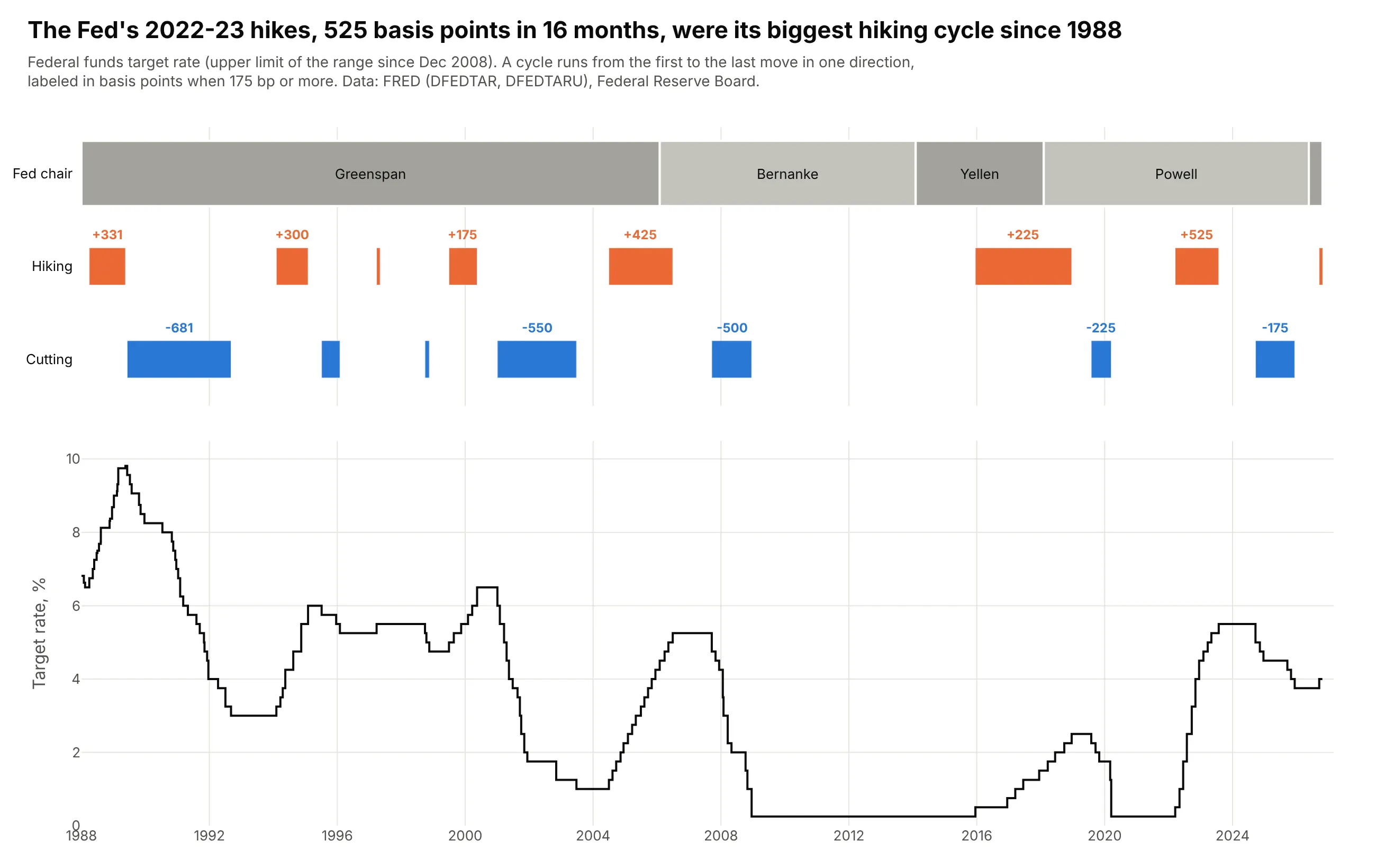
Terms and cycles. From March 2022 to July 2023 the Fed raised its target by 525 basis points in 16 months, its biggest hiking cycle since 1988, and the lanes show which chair ran each cycle above the rate itself. Data: FRED (DFEDTAR, DFEDTARU), Federal Reserve Board list of chairs.

A short history

Joseph Priestley drew the lifespans of famous people as bars on a time axis in his Chart of Biography in 1765, and this is the same idea redrawn with Plotly for 16 scientists and philosophers who died before then:

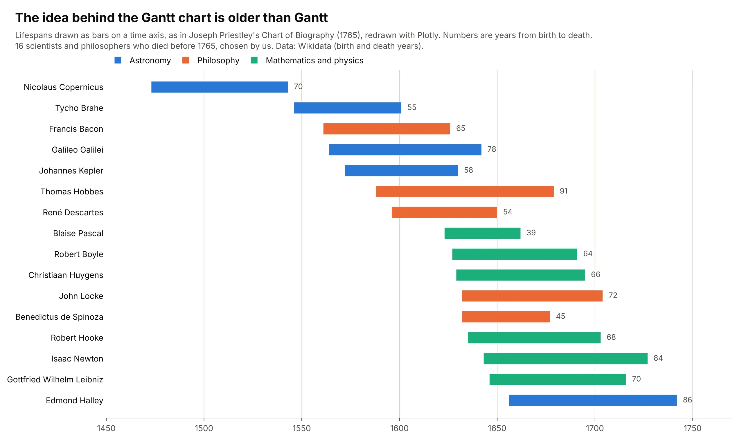
Karol Adamiecki, a Polish engineer, developed a scheduling chart he called the "harmonogram" in 1896 but published it only in 1931, in Polish, so it stayed little known in the West (Marsh, 1975). Henry Gantt developed his charts in the 1910s to schedule production and track progress against plan, and they spread through US industry and government during and after the First World War (Wilson, 2003); the dependency arrows that project software draws today came later, with the critical path method of the late 1950s.

Alternatives to a Gantt chart

Here's the same set of 11 trials drawn six ways. Some are better for the question, some worse, some just different:

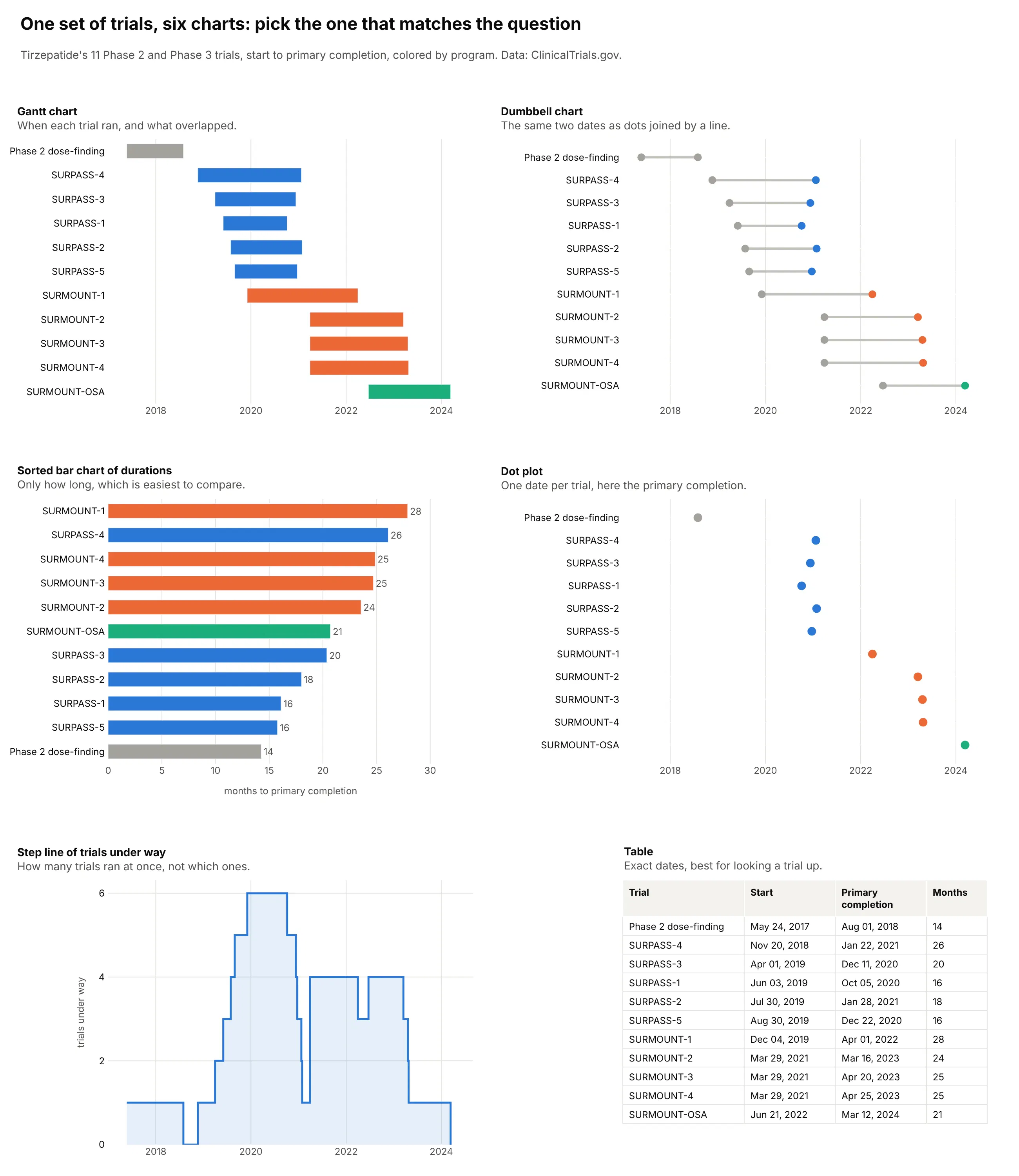
• Sorted bar chart of durations (better when only the length matters). Bars that share a baseline are easier to compare than bars that start on different dates, so this shows at once that SURMOUNT-1 took longest (28 months). You lose the calendar and the overlap.
• Dumbbell chart (works too). The two dates as dots joined by a line carry the same information with less ink, which helps when there are many rows and the overlap matters less than the dates themselves. See our dumbbell chart guide.
• Dot plot (different). One date per item, for deadlines, launches or readouts that have no duration.
• Step line of tasks under way (different). Counts how many tasks were running at each moment, here up to six trials at once from December 2019, which answers a capacity question but no longer says which tasks they were.
• Table (better for looking things up). Exact dates for each row, and the right choice for hundreds of tasks that each need a label, but the pattern over time disappears.

How to make a Gantt chart

With AI

ChatGPT, Claude Code, GitHub Copilot, Cursor and other AI tools are excellent at writing Plotly code. Name Plotly in the prompt, describe the rows, the dates and what color means, and list the details you want:

With Plotly Studio

Plotly Studio is a desktop app where you point an AI at a dataset and it builds charts and a Dash app around your questions. Ask for a Gantt chart the same way:

Show a Gantt chart of our clinical trials, one row per trial from start date to primary completion, grouped and colored by indication. Hatch the part after today, mark FDA approvals as diamonds, and add a dropdown to filter by sponsor.

Make a Gantt chart in Python or JavaScript

This is the code AI tools write under the hood. In Python, px.timeline makes a Gantt chart from a table with a task, a start and an end column:

Under the hood that's a horizontal bar trace whose base is each start date and whose length is the duration in milliseconds, on a date axis. In JavaScript, plotly.js builds the same chart from that bar trace:

The same go.Bar(orientation="h", base=start, x=duration_ms) in Python gives you full control, for several phases in one row, a today line or milestones, which is how every example in this guide is built.

Share it

Every Plotly chart has a Share chart button (the cloud icon in its toolbar) that uploads it to Plotly Cloud and gives you a link. Only you can see it until you change its visibility.

For a live app, put the chart in a Dash app and publish it with the Plotly Cloud CLI. Coding agents can run these commands for you:

If your data has to stay in your own cloud or data center, publish to Dash Enterprise instead.

Dos and don'ts

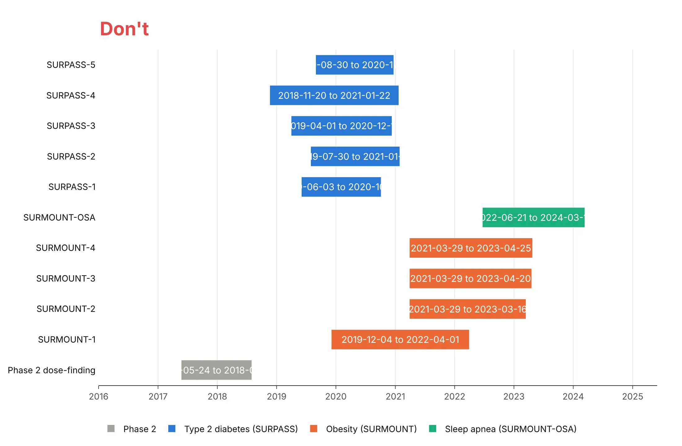
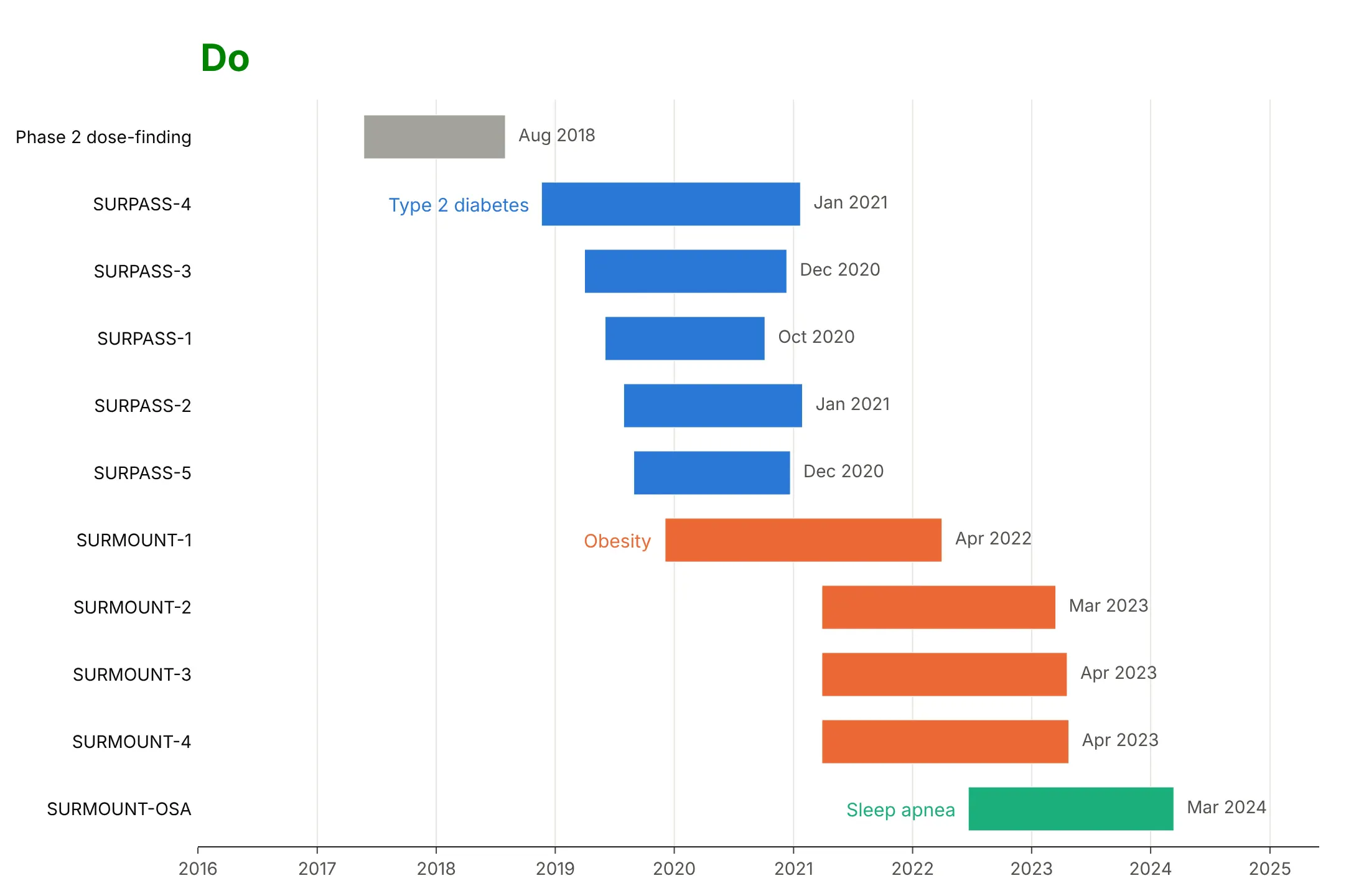
A Gantt chart is easy to get roughly right and easy to make hard to read. Most of the work for a published chart is ordering the rows and choosing what to print on the bars. Here are the 11 tirzepatide trials both ways.

Don't leave the rows in alphabetical order with the first row at the bottom, which scrambles the programs and the sequence, or force full date ranges into every bar, where most of them get cut off:

Do sort the rows by program and start date with the first on top, keep the same colors, name the programs next to their first bar and print the number that matters (here the primary completion month) after each bar:

Use color for one thing

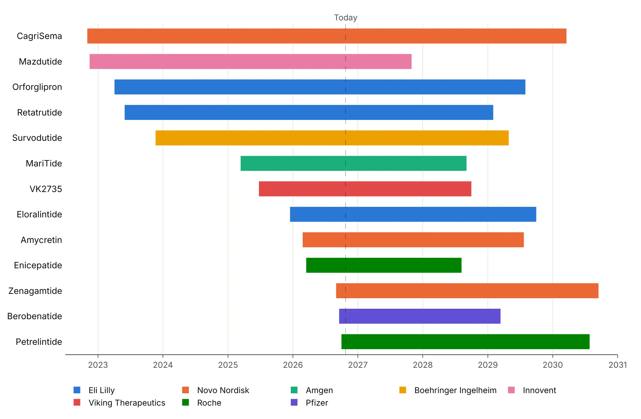
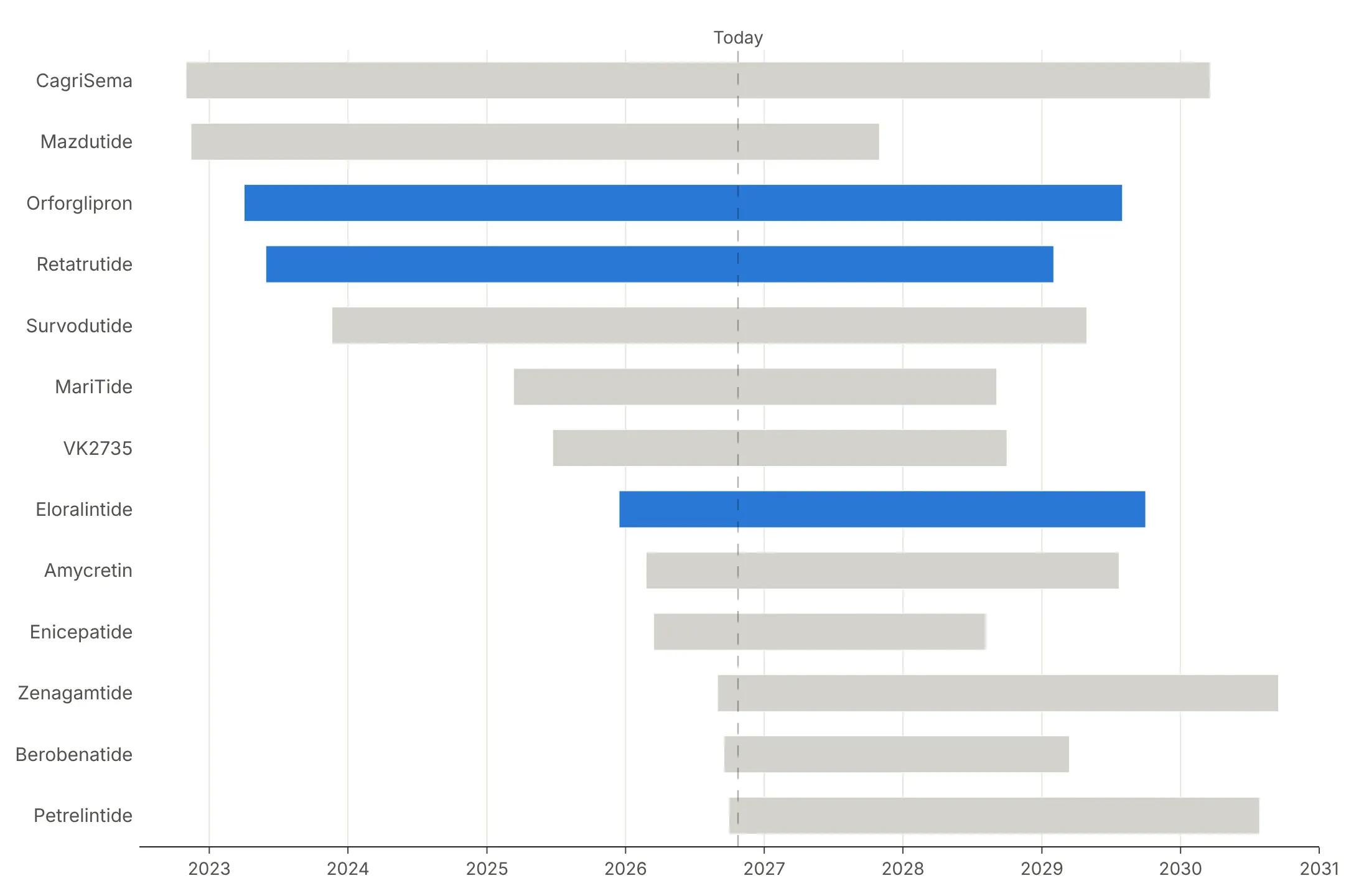
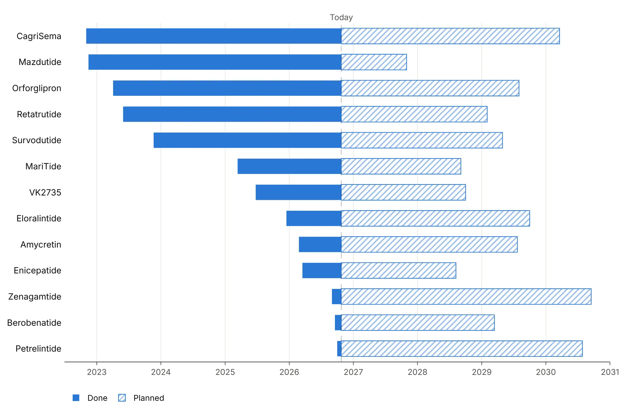
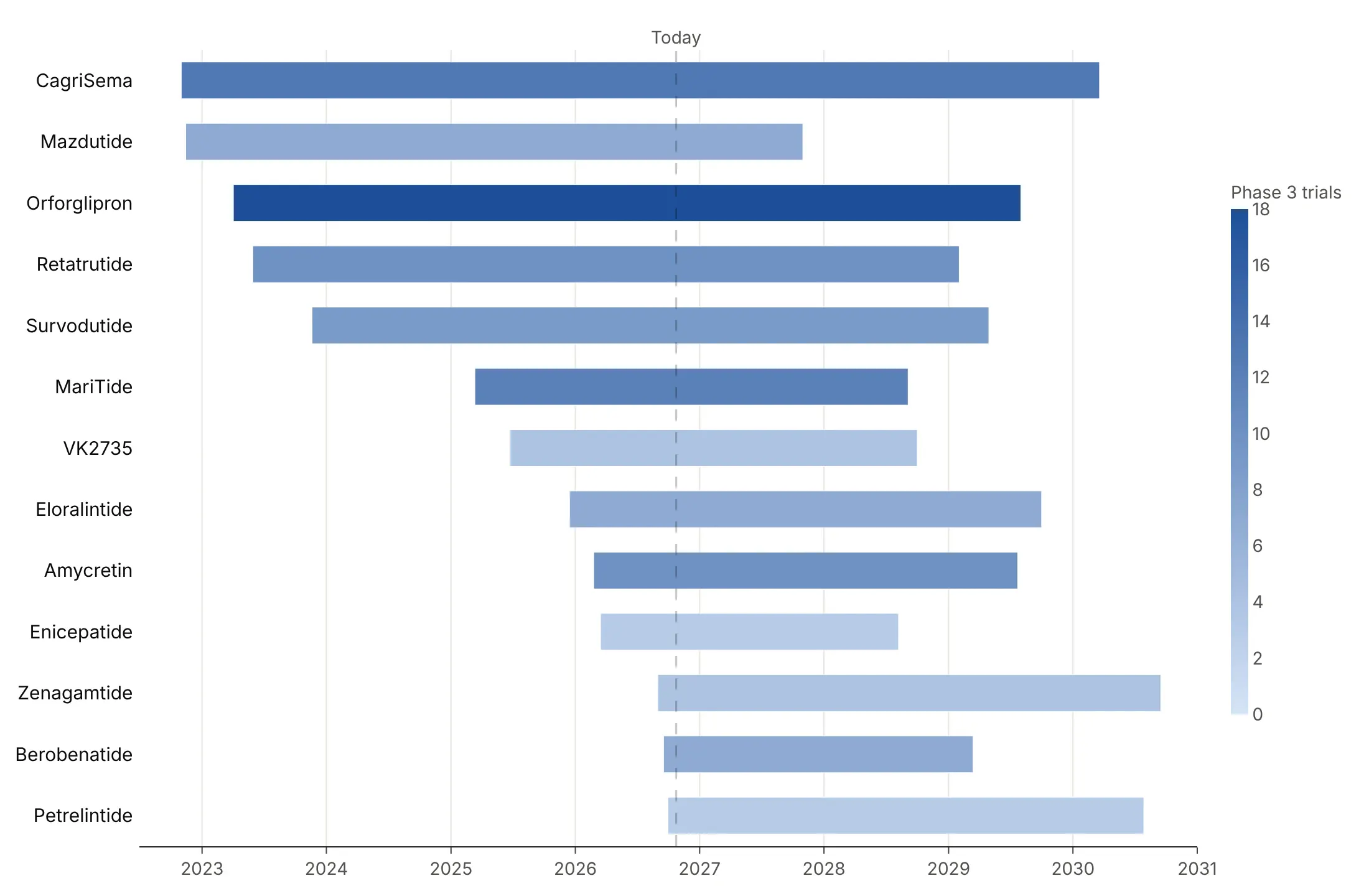
Bar length already shows duration, so color is free to say something else. Here are four options on the same 13 obesity drug programs in Phase 3, each drawn from its first trial start to its last expected readout.

By group. One color per sponsor shows who is behind each program, and it's a good default when there are fewer than about eight groups.

Highlight one story. Eli Lilly's three programs (orforglipron, retatrutide and eloralintide) are blue and the rest are gray, which works when the chart is about one sponsor.

By status. Each bar is solid up to today and hatched after, so the chart separates what has happened from what is planned.

By a measure. A blue scale by the number of Phase 3 trials shows that orforglipron has the most (18), at the cost of a colorbar the reader has to look up.

Checklist

Do

• Sort the rows by start date, by group or by end date, depending on the question, and set yaxis.autorange="reversed" so the first task is on top.
• Color by group, status or a measure.
• Draw a today line whenever the chart mixes past and future, and hatch the planned part with marker.pattern.
• Mark milestones with diamonds and label them directly.
• Print the number that matters at the end of each bar: an end date, a duration or a count.
• Write a title that states the takeaway, with the source in a muted subtitle.

Don't

• Give every task its own color, which makes an unreadable legend and slows the chart down (see the FAQ).
• Leave rows in alphabetical order unless readers will look tasks up by name.
• Squeeze long labels such as full date ranges inside the bars, where they get clipped. Print one short number after each bar instead.
• Draw hundreds of dependency arrows. Draw the few that explain the schedule.
• Label every row of a chart with 100 or more rows. Hide the tick labels and annotate the outliers instead.

Options to customize

These are the options that matter most for a Gantt chart built from go.Bar (or px.timeline) and the layout. The full list is in the Plotly Gantt chart documentation and the bar reference.

1. px.timeline(x_start=, x_end=, y=, color=): builds the bars from start and end columns; color by a group, not by task.
2. go.Bar(orientation="h", base=start, x=duration_ms): a bar from the start date with the duration in milliseconds, for full control and several phases per row.
3. xaxis.type="date": a date axis for the bars, needed when you build them by hand.
4. yaxis.autorange="reversed": puts the first task on top, which you almost always want.
5. yaxis.categoryorder="array", categoryarray: fixes the row order, by start, group or end.
6. barmode="overlay": keeps several segments of one task on the same row.
7. width: bar thickness, one value per bar if you pass a list, so it can carry a measure such as capacity.
8. marker.pattern.shape: hatching for planned or estimated parts.
9. marker.opacity: per-bar transparency, to fade finished or expired rows.
10. go.Scatter(marker_symbol="diamond"): milestone markers for approvals, launches and deadlines.
11. fig.add_vline or fig.add_shape(type="line", yref="paper"): a today line or a deadline across the chart.
12. fig.add_annotation(ax=, ay=, axref="x", ayref="y"): an arrow between two points in data coordinates, for dependencies.
13. fig.add_vrect: a shaded band across all rows, for recessions, freezes or holidays.
14. make_subplots(shared_xaxes=True): a Gantt chart and a line chart on one time axis.
15. textposition, insidetextanchor: labels inside or after the bars.
16. hovertemplate, customdata: hover content such as exact dates, counts and IDs.

More Gantt chart examples

Eight more Gantt charts built from real public data, each with its source, the technique that makes it work and a prompt to rebuild it.

1. The race for the next obesity drug

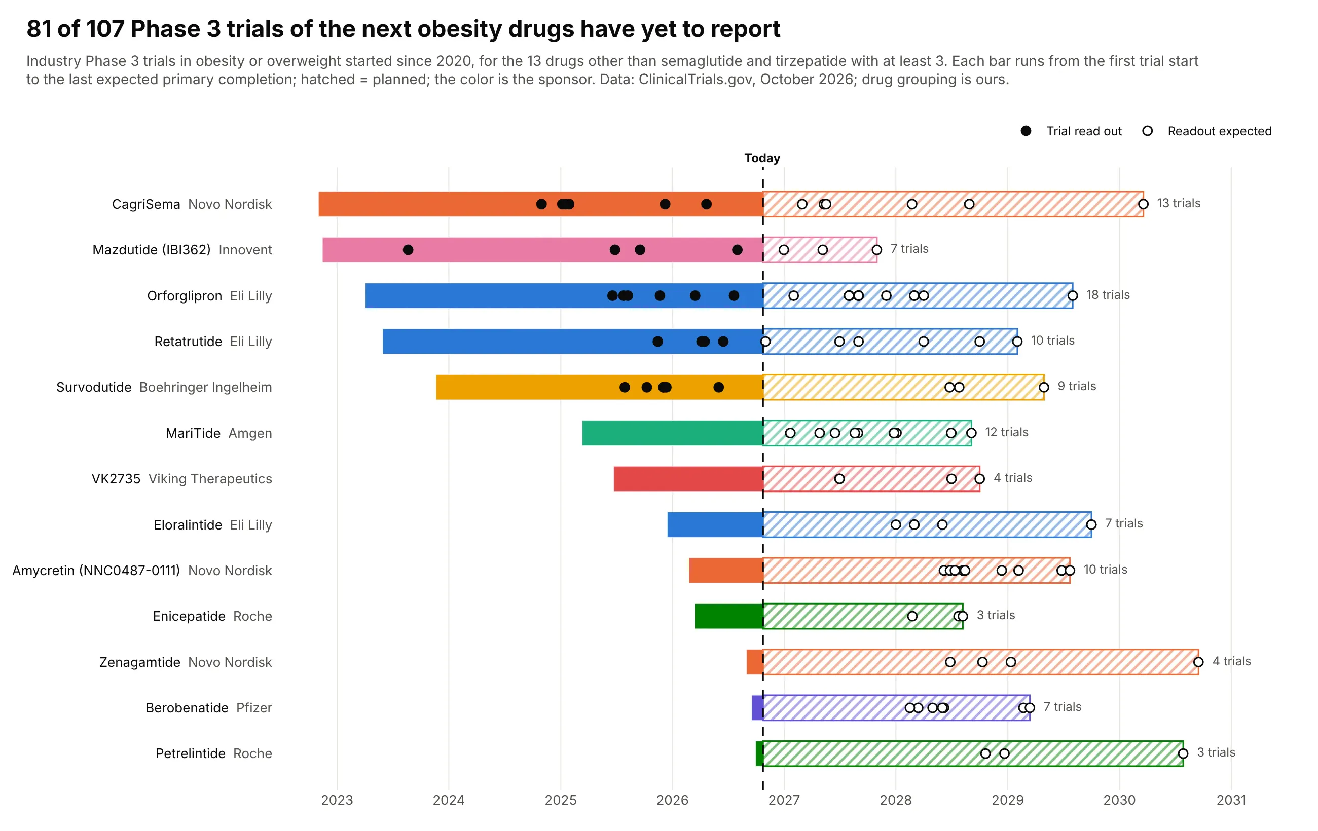
Thirteen obesity drugs other than semaglutide and tirzepatide have 107 industry Phase 3 trials registered since 2020, and 81 of them have yet to reach their primary completion. Lilly's orforglipron has the most trials (18), and readouts run into 2030. Data: ClinicalTrials.gov, October 2026 (grouping by drug is ours).

Tip: roll many tasks up into one bar per program and keep the detail as dots, filled when done and hollow when expected.

2. When Medicare's top drugs lose patent protection

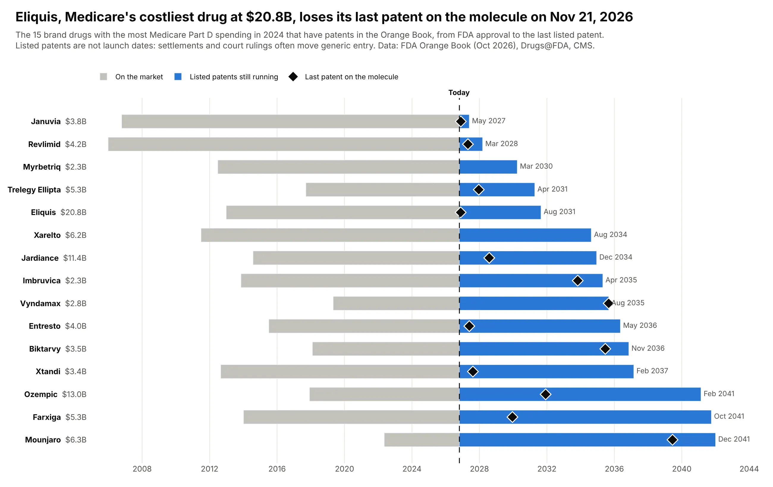
Eliquis cost Medicare Part D $20.8 billion in 2024, more than any other drug, and its last patent on the molecule itself expires on November 21, 2026. Later patents run to 2031, and for Ozempic, Farxiga and Mounjaro they reach 2041. Data: FDA Orange Book (October 2026), Drugs@FDA, CMS Part D Spending by Drug.

Tip: sort by the end date so the chart reads as a calendar of patent cliffs, and put the spending in the row label.

3. How long it took to build every US nuclear reactor

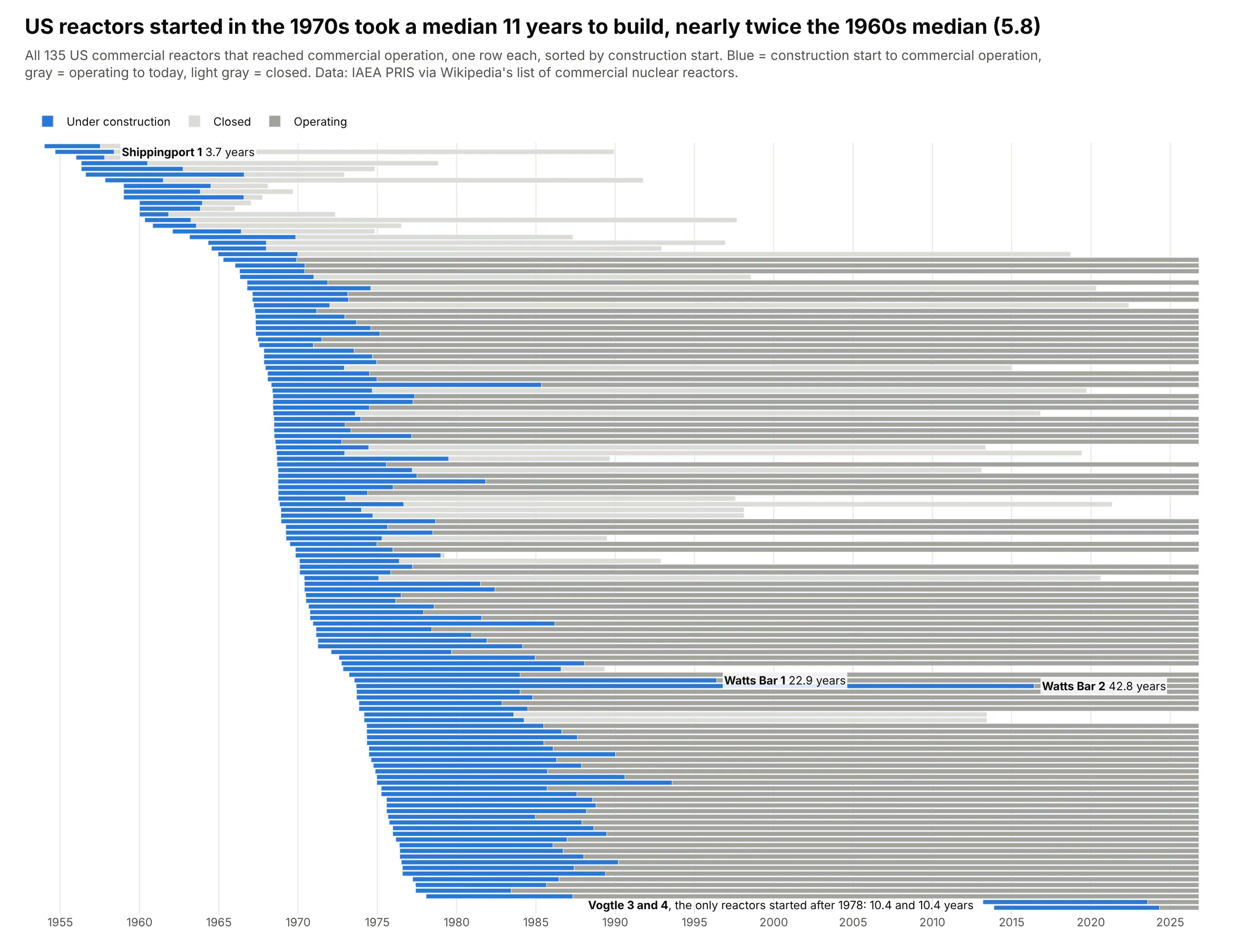
US reactors started in the 1960s took a median 5.8 years to build, and those started in the 1970s took 11. Watts Bar 2 took 42.8 years, and Vogtle 3 and 4, the only reactors started after 1978, took 10.4 years each. Data: IAEA PRIS via Wikipedia's list of commercial nuclear reactors.

Tip: for 100+ rows, set bargap=0, hide the tick labels and annotate only the outliers.

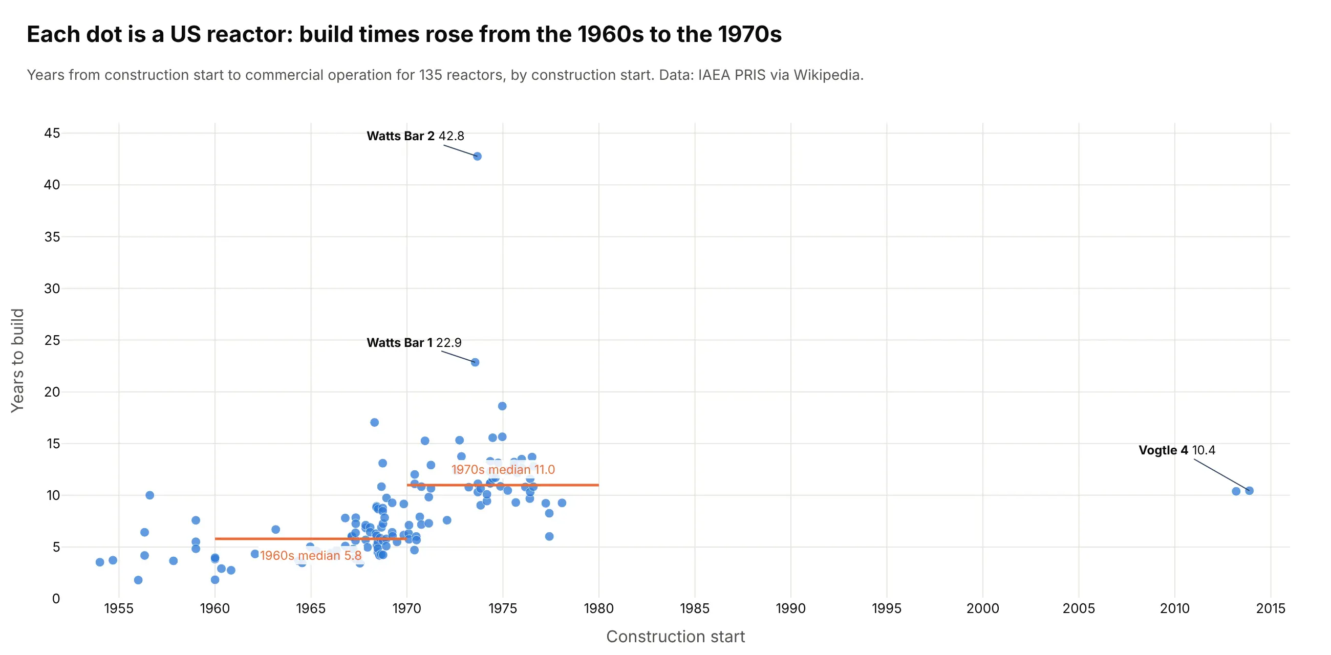
Another way to see it: a scatter of build time against construction start shows the same jump as two medians, but loses the operating lives.

4. Every S&P 500 bear market since 1950, side by side

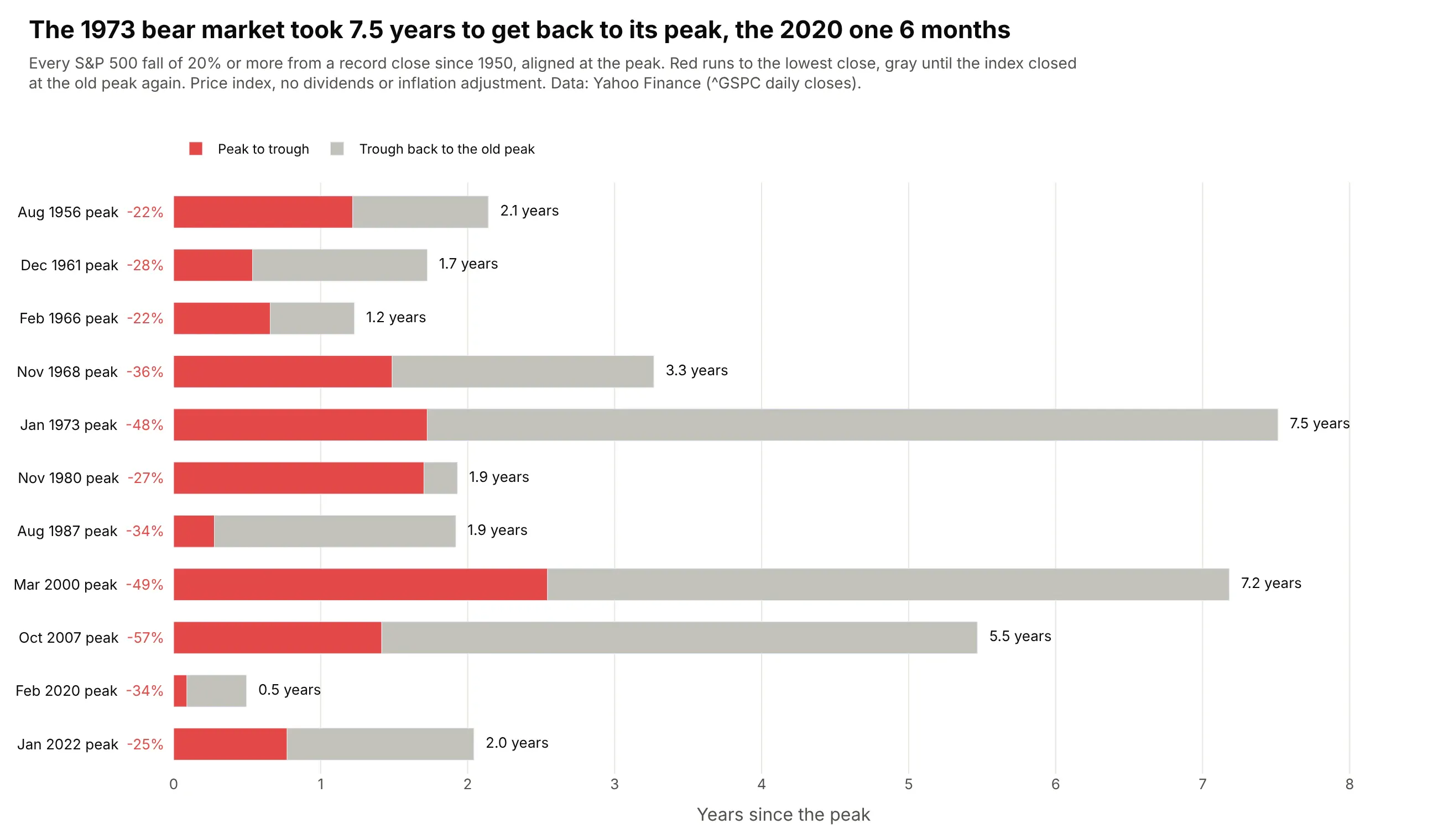
Aligned at the peak, the 11 bear markets since 1950 range from 6 months peak to peak (2020) to 7.5 years (1973). The 2000 and 2007 falls took 7.2 and 5.5 years to win back. Data: Yahoo Finance, S&P 500 daily closes (price only).

Tip: a Gantt chart doesn't need dates: use base=0 and lengths in years to compare episodes from different decades.

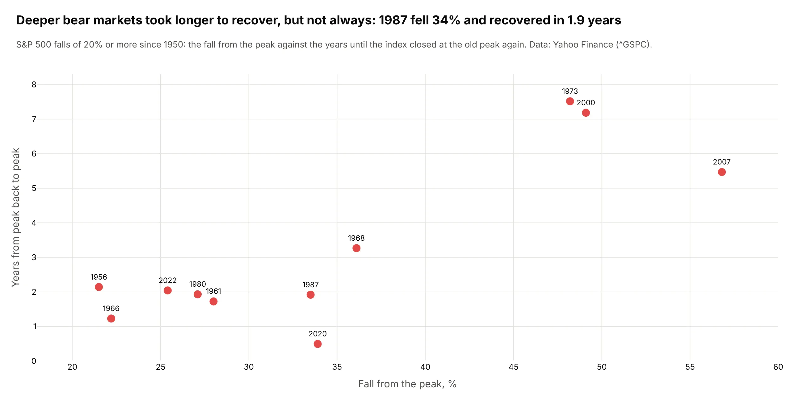
Another way to see it: a scatter of the fall against the recovery time shows that depth predicts duration loosely: 1987 fell 34% and recovered in 1.9 years.

5. Presidents and recessions on one timeline

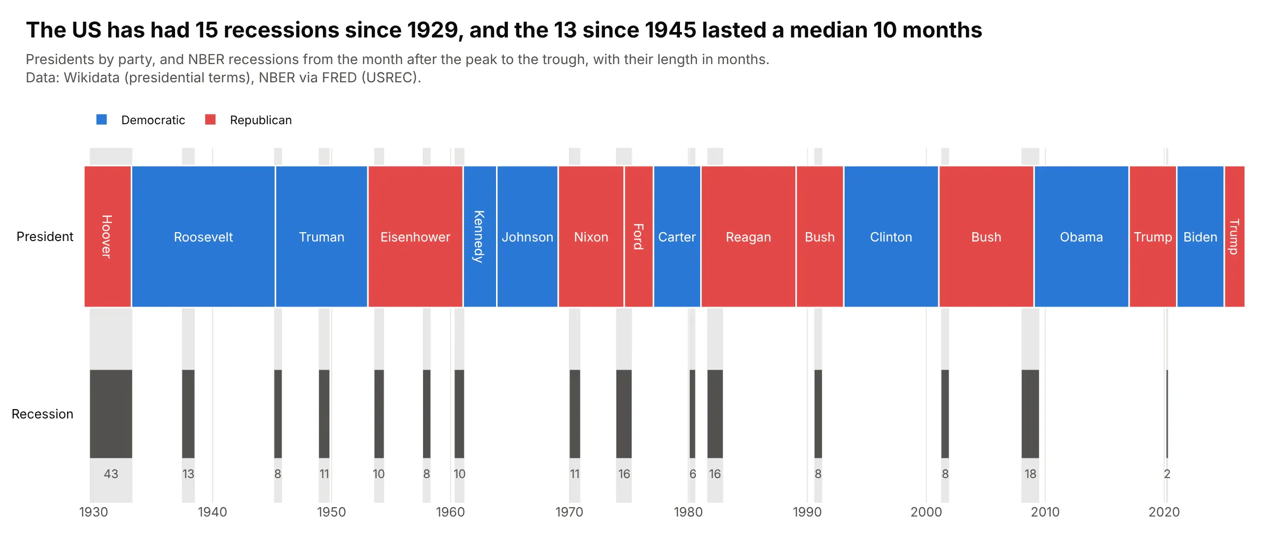
The US has had 15 recessions since 1929, and the 13 since 1945 lasted a median 10 months. The longest since then ran 18 months (2008-09) and the shortest 2 months (2020). Data: Wikidata (presidential terms), NBER recession dates via FRED (USREC).

Tip: a one-row Gantt chart is a timeline; fig.add_vrect shades each event across every row.

6. Who has lived on the International Space Station

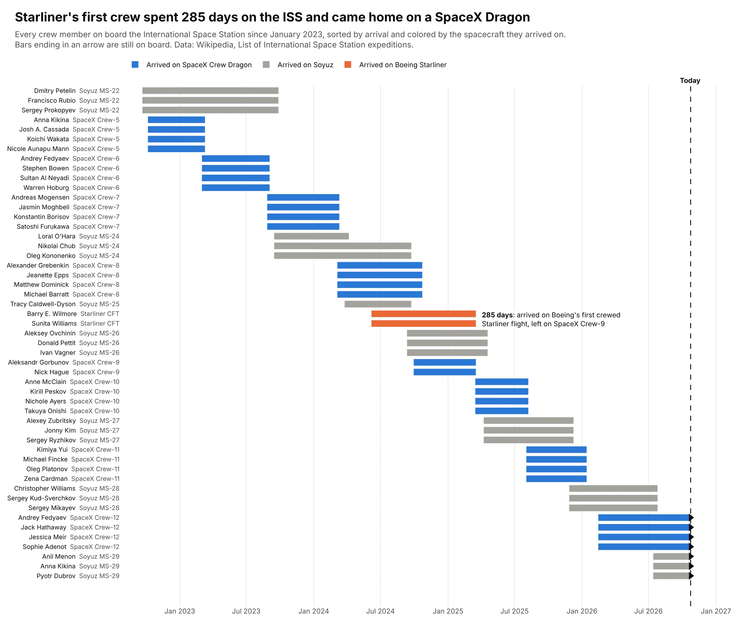
Barry Wilmore and Sunita Williams arrived on Boeing's first crewed Starliner flight in June 2024 and left 285 days later on SpaceX Crew-9. Seven people are on board today. Data: Wikipedia, List of International Space Station expeditions.

Tip: sort by arrival so each crew forms a block, and end open stays at today with an arrow marker.

7. Every plotly.py release, by major version

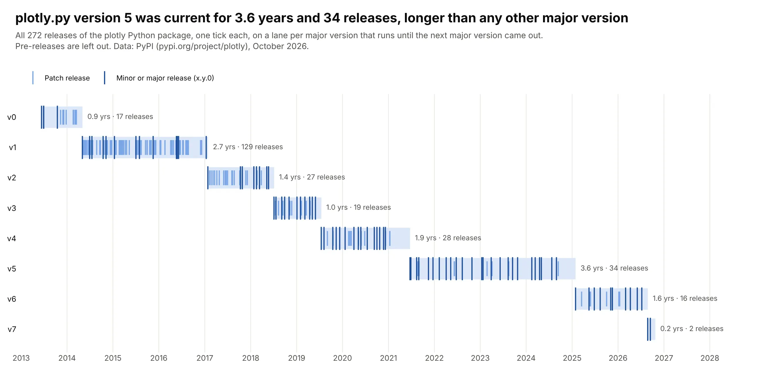
plotly.py has shipped 272 releases since 2013, and version 5 stayed current for 3.6 years and 34 releases, longer than any other major version. Version 7 came out in August 2026. Data: PyPI (pypi.org/project/plotly).

Tip: marker.symbol="line-ns" draws events as ticks on a lane, a light way to show many milestones.

8. Every team's run at the 2026 World Cup

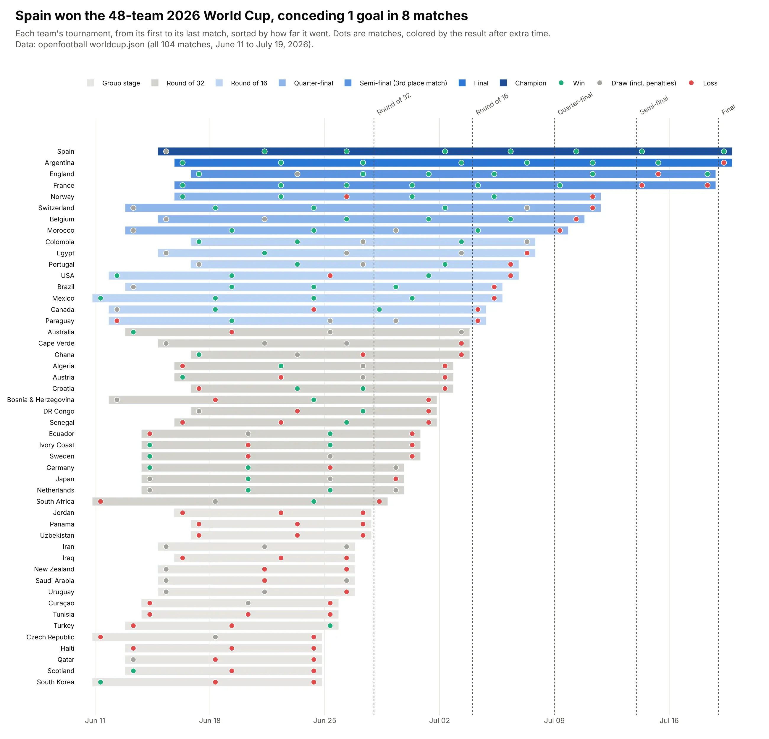
Sorted by how far each team went, the 48 bars step down like a bracket. Spain won 7 of 8 matches and conceded once, beating Argentina 1-0 after extra time in the final. Data: openfootball worldcup.json (all 104 matches).

Tip: sort rows by outcome and put each event on its bar as a colored dot, so one chart shows schedule and results.