Chris Parmer

October 24, 2026

Kaplan-Meier Curves - A Complete Guide

TL;DR

A Kaplan-Meier curve shows the share of a group that hasn't had an event yet (death, relapse, failure, closing a ticket) at each point in time, as a step line that drops at every event.
Kaplan-Meier curves are also known as Kaplan-Meier plots and survival curves, and are similar to cumulative incidence curves and ECDF plots.
It handles censoring: people or things still event-free when you stopped watching count for as long as you watched them, instead of being dropped or counted as events.
Read the median where the curve crosses 50%, compare groups with a log-rank test, and put a number-at-risk table under the chart so readers know how much data is behind the tail.
You can make a Kaplan-Meier plot with Plotly from go.Scatter with line_shape="hv", plus a fill="tonexty" confidence band and tick markers for censored subjects; the short helper below does it.

What is a Kaplan-Meier curve?

Kaplan-Meier curves look like this:

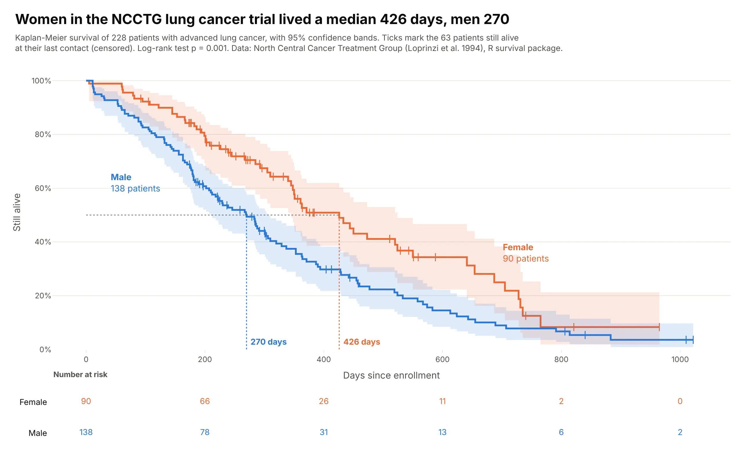
Kaplan-Meier survival curves with 95% confidence bands for 228 patients with advanced lung cancer in the NCCTG trial. Women (90 patients, orange) lived a median 426 days and men (138, blue) 270 days; tick marks show the 63 patients still alive at last contact, and a number-at-risk table under the chart falls from 90 and 138 at day 0 to 0 and 2 at day 1,000. Log-rank p = 0.001

Data: North Central Cancer Treatment Group (Loprinzi et al. 1994), the lung dataset in R's survival package.

How do you read a Kaplan-Meier curve? In the example above, notice these things:

Each line is one group of patients, men in blue and women in orange, and its height is the share still alive on each day since enrollment. Both lines start at 100% and step down each time a patient in that group dies.
The dotted lines drop from where each curve crosses 50% to that group's median survival. The orange line gets there at 426 days, much later than the blue one, so women in this trial lived longer.
The small vertical ticks are censored patients, meaning they were still alive at their last contact. They count as at risk until that day and then leave the curve without pulling it down.
The shaded bands are 95% confidence intervals, and they get wider toward the right as fewer patients are left. The orange and blue bands overlap for the first few months and again after about day 650, so the clearest difference between the groups is in between.
Read the number-at-risk table under the chart before you trust the right end of a curve. By day 800 only a handful of women were still being followed, so the last drops of the orange line rest on very few people.

It's often used for charts like these:

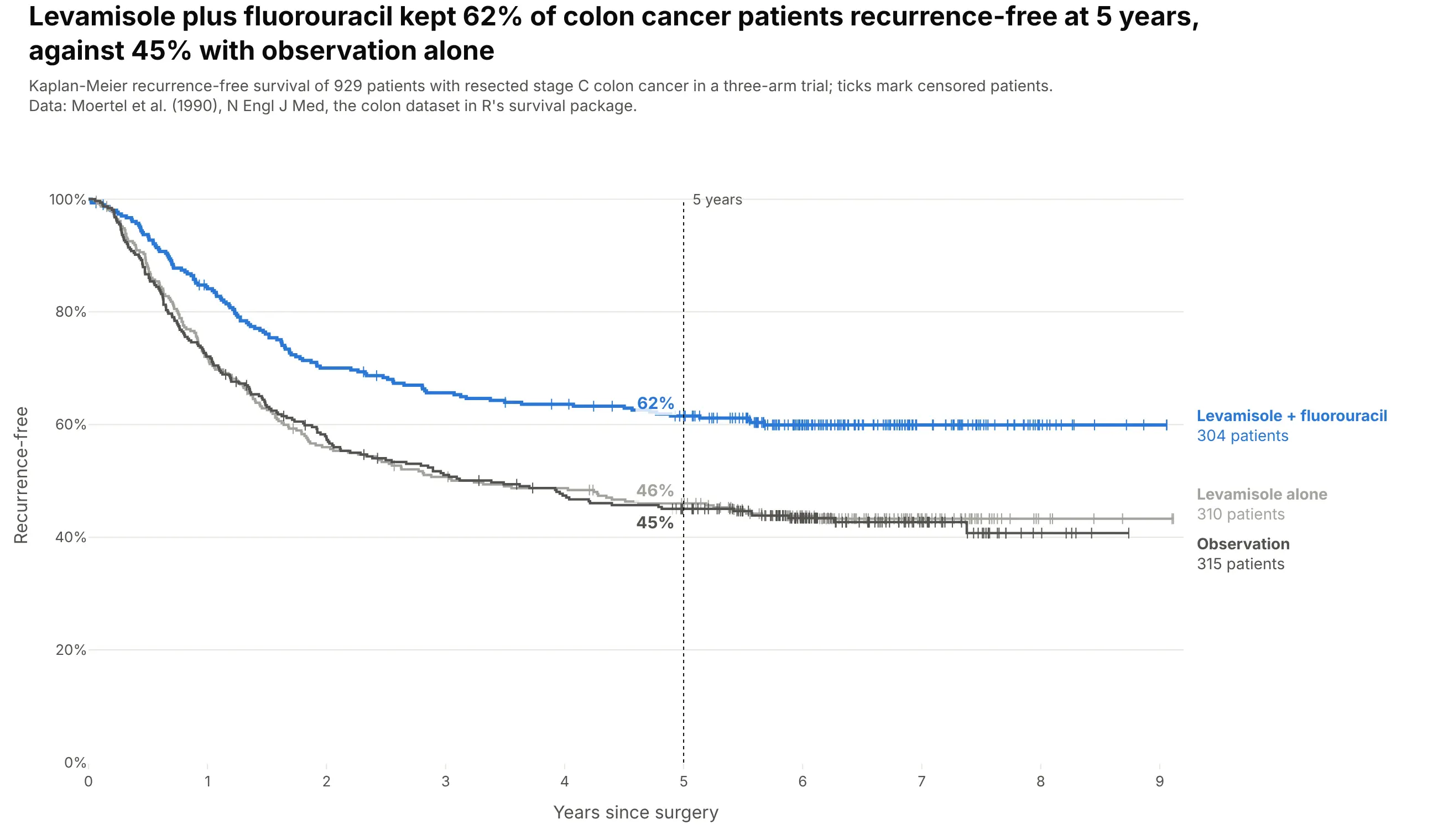
Kaplan-Meier recurrence-free survival for three arms of a stage C colon cancer trial over nine years: levamisole plus fluorouracil kept 62% of patients recurrence-free at 5 years, against 46% with levamisole alone and 45% with observation

A clinical trial readout. Levamisole plus fluorouracil kept 62% of 304 colon cancer patients recurrence-free at five years, against 45% with observation alone. Data: Moertel et al. (1990), the colon dataset in R's survival package.

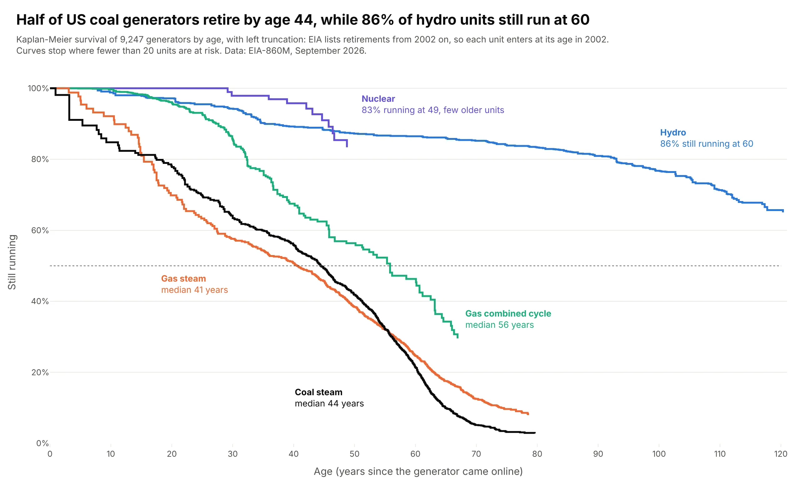
Kaplan-Meier curves of US power generators still running by age, for five technologies. Half of coal steam units retire by age 44, gas steam by 41 and gas combined cycle by 56, while 86% of hydro units still run at 60 and 83% of nuclear units run at 49

The lifetime of equipment. Half of US coal generators retire by age 44, while 86% of hydro units are still running at 60. Data: EIA-860M, September 2026.

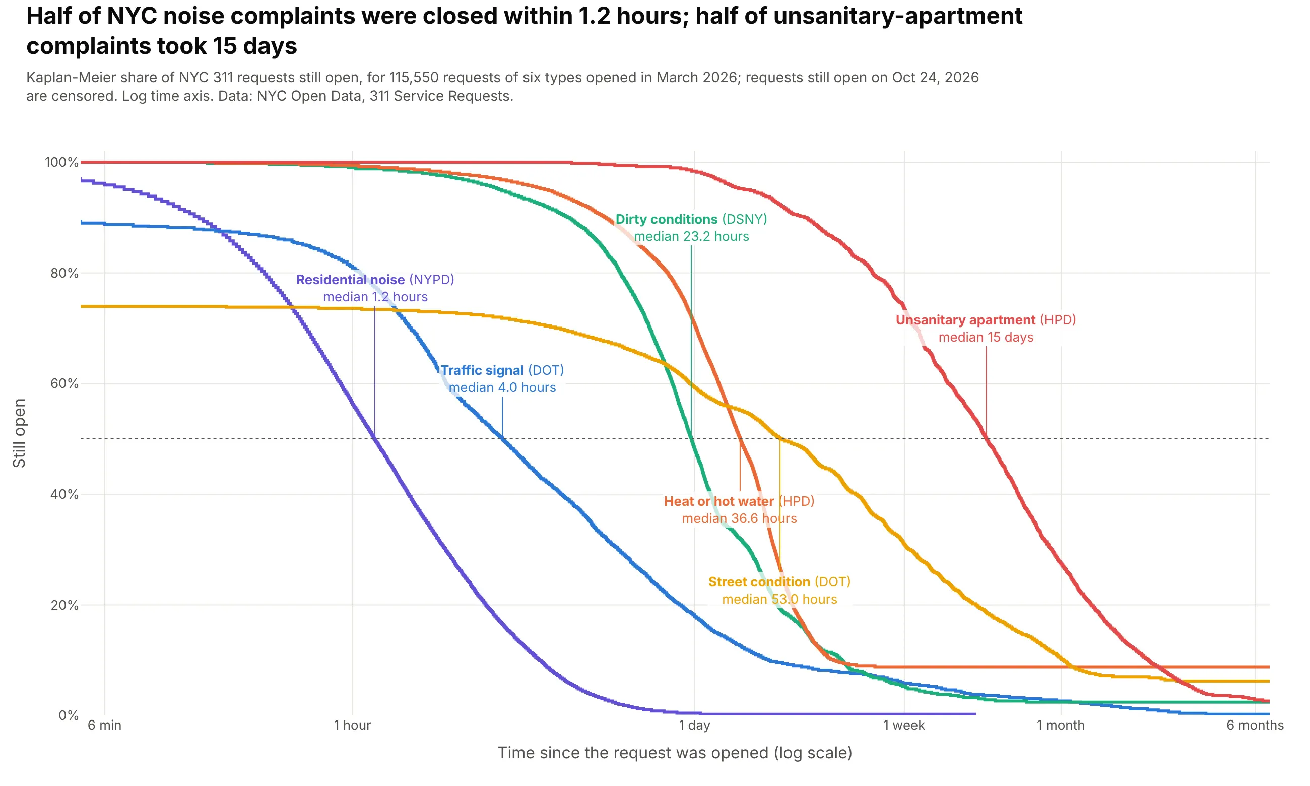
Kaplan-Meier curves of NYC 311 requests still open, for six complaint types on a log time axis from minutes to six months. Residential noise complaints close in a median 1.2 hours, traffic signals 4.0 hours, dirty conditions 23.2 hours, heat or hot water 36.6 hours, street conditions 53 hours and unsanitary apartments 15 days

Time to resolve something. Half of March's NYC noise complaints were closed within 1.2 hours, and half of unsanitary-apartment complaints took 15 days. Data: NYC Open Data, 311 Service Requests.

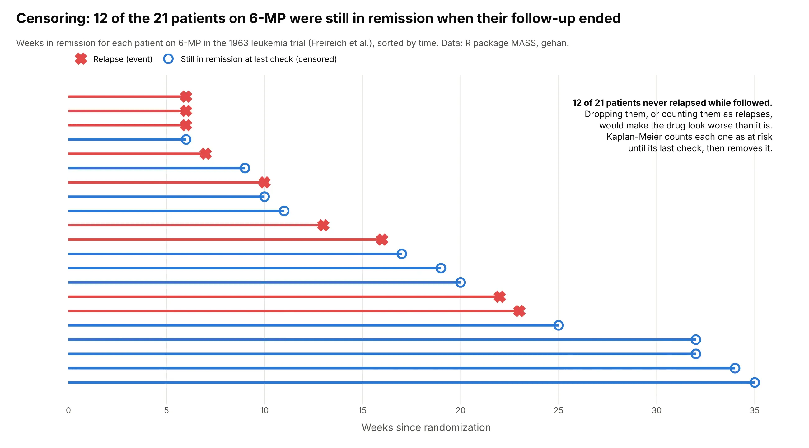
Every curve in this section keeps the patients, generators and complaints that hadn't had their event yet when the data was collected, and counts them only for as long as they were followed. That handling of unfinished follow-up, called censoring, is what makes this chart different from a histogram or a line of averages:

Each of the 21 patients on 6-MP in the 1963 leukemia trial as a horizontal line from 0 to their last week of follow-up, sorted by length. Nine lines end in a red X for a relapse and twelve end in a blue circle because the patient was still in remission when follow-up ended

A short history

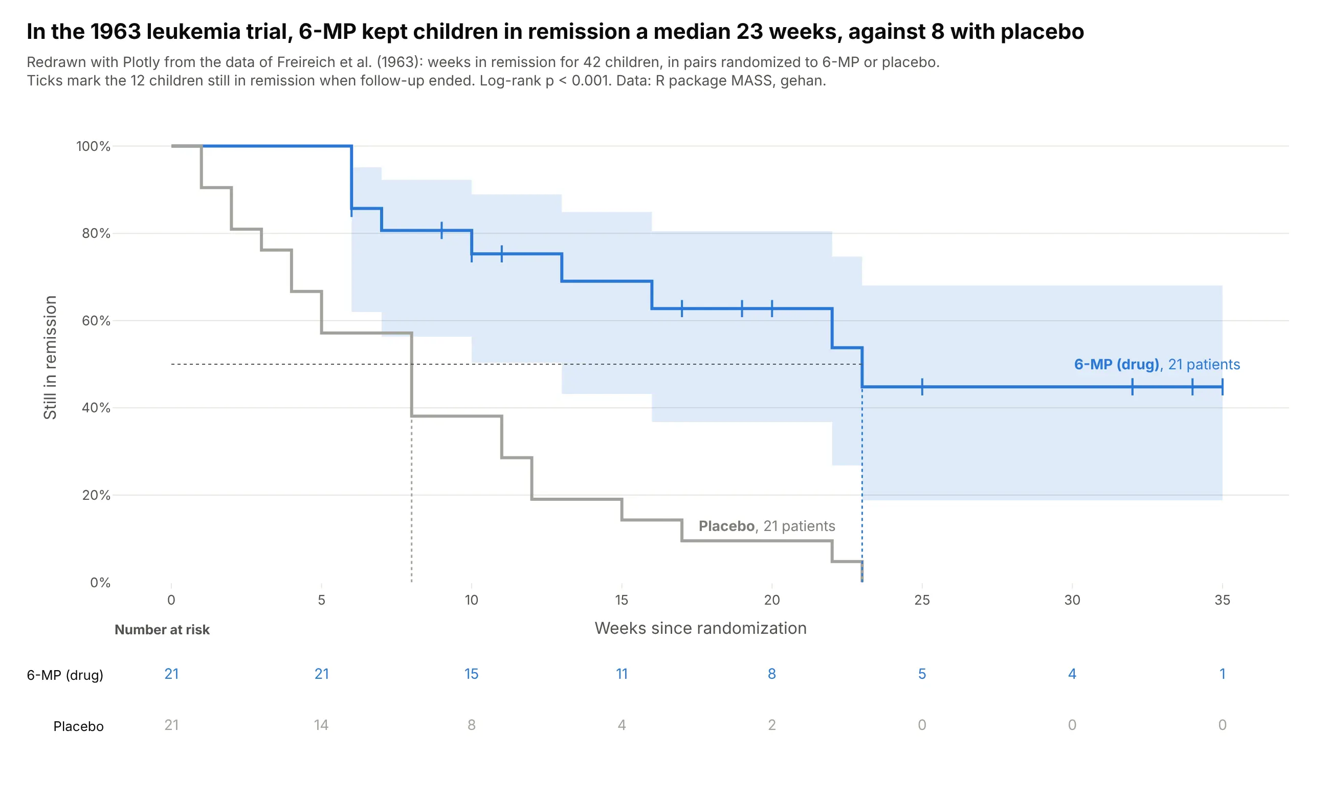
Edward Kaplan and Paul Meier published the estimator in 1958 in the Journal of the American Statistical Association, as a way to estimate survival from "incomplete observations". Its confidence intervals use Major Greenwood's 1926 variance formula, and the log-rank test that compares two curves came from Nathan Mantel (1966) and was named by Peto and Peto (1972). The classic teaching example is the 1963 trial of 6-MP for childhood leukemia by Freireich et al., which Gehan (1965) used to compare censored survival curves, redrawn here with Plotly:

The 1963 6-MP leukemia trial redrawn with Plotly as Kaplan-Meier curves: 21 children on 6-MP stayed in remission a median 23 weeks, with 12 censored, against 8 weeks for 21 on placebo, all of whom relapsed. A number-at-risk table shows 21, 14, 8 and 4 placebo patients at weeks 0, 5, 10 and 15

Alternatives to a Kaplan-Meier curve

Here's the same lung cancer survival data drawn six ways. Some are better for the question, some worse, some just different:

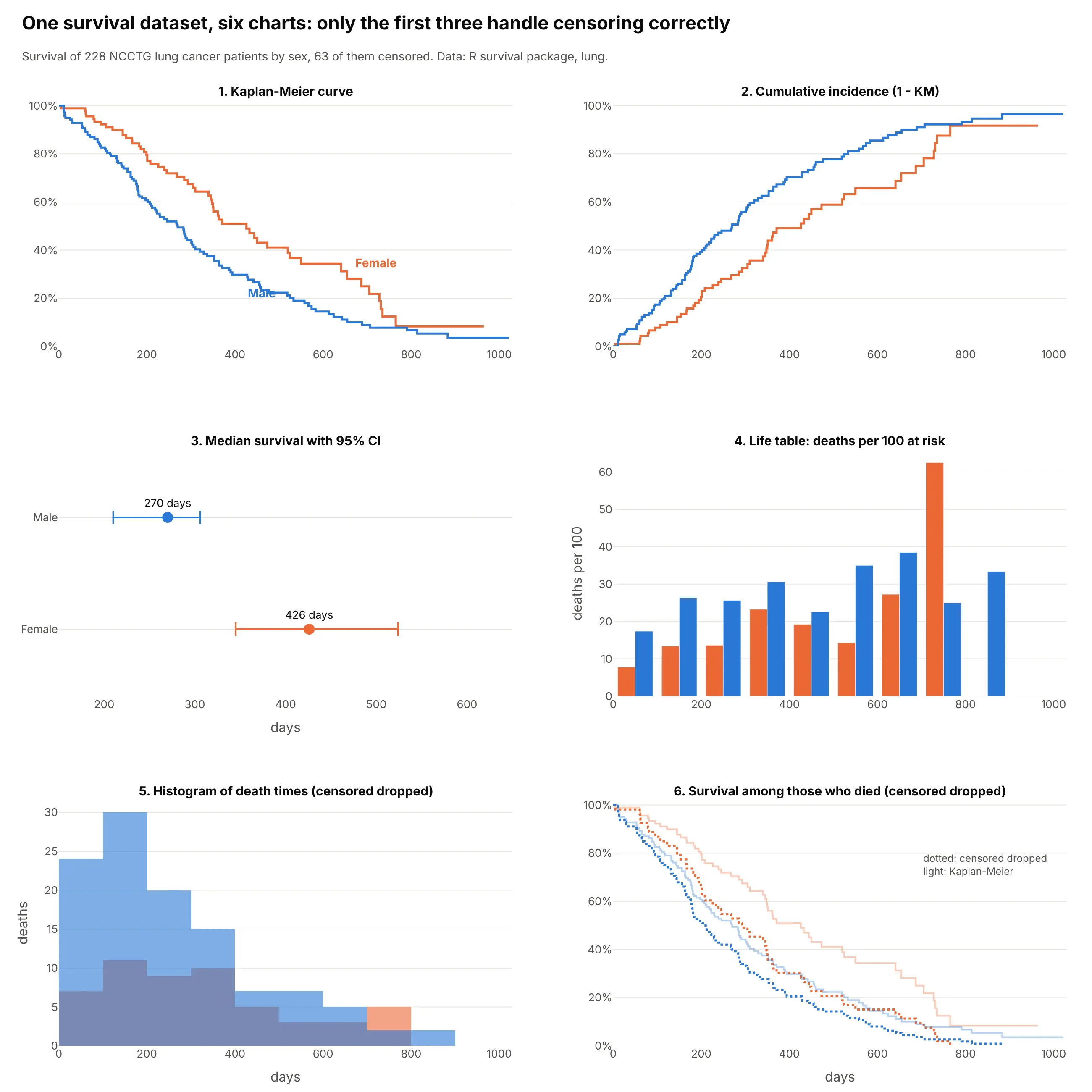
The NCCTG lung cancer data drawn six ways: Kaplan-Meier curves by sex; the same curves flipped as cumulative incidence; median survival of 270 days for men and 426 for women with 95% intervals; a life table of deaths per 100 patients at risk in each 100-day interval; a histogram of death times with censored patients dropped; and survival among only the patients who died, which falls below the Kaplan-Meier curves

Kaplan-Meier curve (the default). It shows the whole time course, handles censoring and gives the median and any landmark (1-year, 5-year) in one chart.
Cumulative incidence, 1 - KM (works too). The same estimate drawn rising, which reads better when the event is the thing you count, such as recurrences or results reported (example 4).
Median survival with a confidence interval (works too, for a summary). One number per group fits a table or a forest plot, but it hides when the curves separate or cross.
Life table (different). Deaths per 100 at risk in fixed intervals shows how the risk changes over time, which the curve only shows as its slope. The last intervals rest on very few patients and jump around.
Histogram of event times (worse). It drops the 63 censored patients, so it describes only those who died and overstates how fast deaths happen.
Survival among those who died (worse). Dropping censored patients and drawing a curve of the rest puts women's median at 293 days instead of 426, and men's at 207 instead of 270.

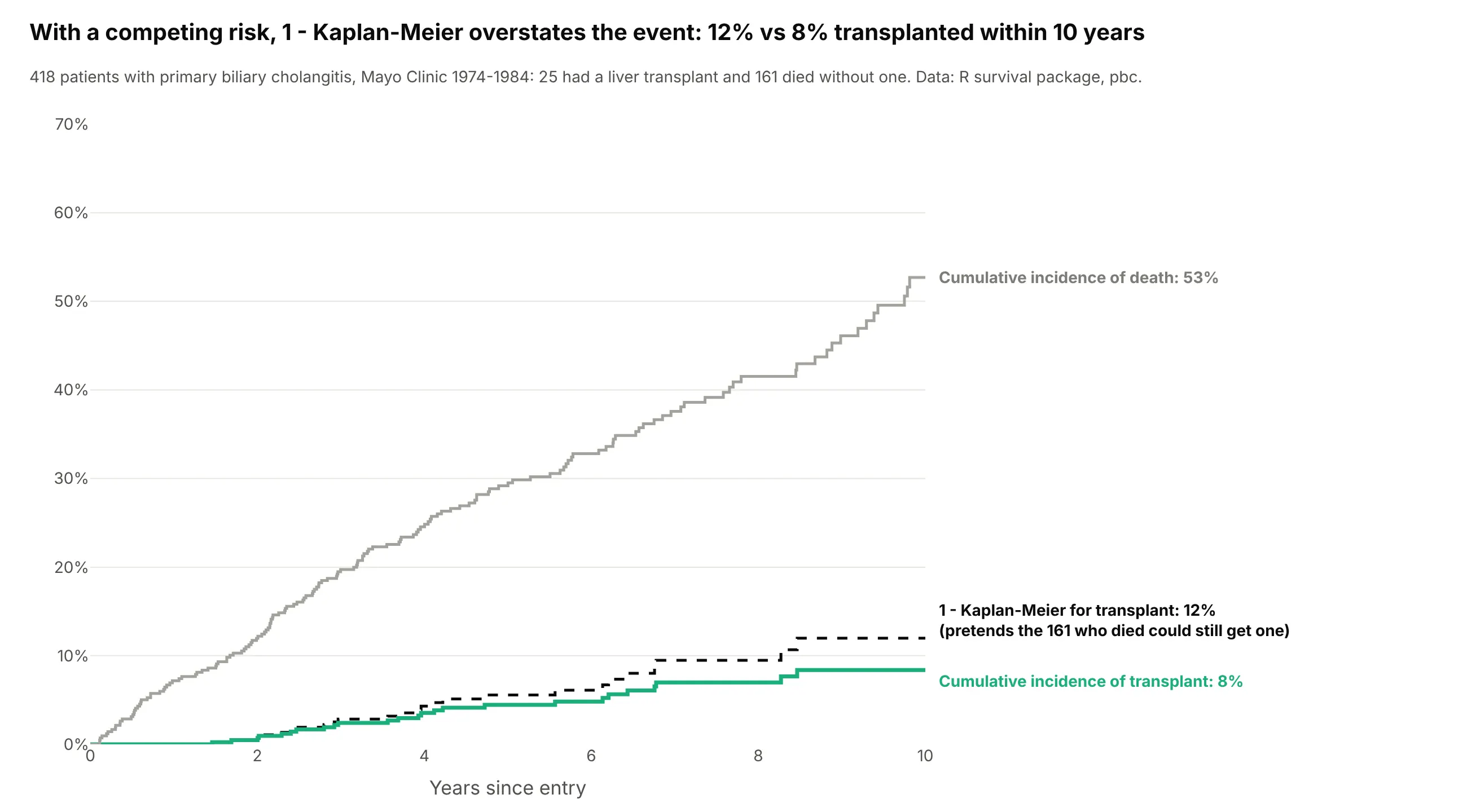
When something else can happen first, a competing risk, 1 - KM overstates the event and a cumulative incidence curve is the right chart. In the Mayo liver study, patients who died could no longer get a transplant:

Cumulative incidence of liver transplant and of death over 10 years for 418 patients with primary biliary cholangitis. 1 minus Kaplan-Meier for transplant reaches 12%, because it treats the 161 deaths as if those patients could still get a transplant, while the Aalen-Johansen cumulative incidence of transplant is 8% and of death 53%

How to make a Kaplan-Meier curve

With AI

ChatGPT, Claude Code, GitHub Copilot, Cursor and other AI tools are excellent at writing Plotly code. Name Plotly in the prompt, say which column is the time, which is the event and how censoring is coded, and list the checks you want:

Make a plotly Kaplan-Meier survival plot from patients.csv
(columns: patient_id, arm, days, died where 1 = died and 0 = censored).

- Compute the Kaplan-Meier estimate per arm with numpy (or lifelines) and draw it as
  go.Scatter with line_shape="hv", starting at 100% on day 0.
- 95% Greenwood confidence band per arm with fill="tonexty" in a light tint.
- Tick marks (marker symbol "line-ns-open") at each censored patient's time, on the curve.
- Stop each curve when fewer than 10 patients are at risk.
- Dotted lines at the medians, labeled in days; label curves directly, no legend.
- A number-at-risk table under the chart in a second subplot row with a shared x axis.
- Log-rank p-value in the subtitle. Check the medians against lifelines.
- Inter font, white background, y axis 0-100%. Save as km.html and a PNG at 2x scale.

With Plotly Studio

Plotly Studio is a desktop app where you point an AI at a dataset and it builds charts and a Dash app around your questions. Ask for a survival curve the same way:

Show Kaplan-Meier survival curves of time to churn by subscription plan, with censoring ticks, 95% bands and a number-at-risk table, and a dropdown to switch the grouping between plan, region and signup year.

Make a Kaplan-Meier curve in Python or JavaScript

This is the code AI tools write under the hood. The helper computes the estimate with numpy and draws each group with Plotly as step lines, a band and censoring ticks:

import numpy as np
import pandas as pd
import plotly.graph_objects as go


def km(time, event):
    """Kaplan-Meier estimate with a 95% Greenwood band (log-log scale)."""
    t, e = np.asarray(time, float), np.asarray(event, int)
    u, d = np.unique(t[e == 1], return_counts=True)           # event times, deaths at each
    n = len(t) - np.searchsorted(np.sort(t), u)               # number still at risk
    s = np.cumprod(1 - d / n)
    with np.errstate(divide="ignore", invalid="ignore"):
        se = np.sqrt(np.cumsum(d / (n * (n - d)))) / np.abs(np.log(s))
    lo, hi = np.nan_to_num(s ** np.exp(1.96 * se)), np.nan_to_num(s ** np.exp(-1.96 * se))
    return pd.DataFrame({"time": np.r_[0, u, t.max()], "surv": np.r_[1, s, s[-1]],
                         "lo": np.r_[1, lo, lo[-1]], "hi": np.r_[1, hi, hi[-1]]})


def make_km_plot(df, time, event, group, colors=("#2a78d6", "#eb6834", "#1baf7a")):
    fig = go.Figure()
    for (name, d), c in zip(df.groupby(group), colors):
        tab = km(d[time], d[event])
        fig.add_scatter(x=tab.time, y=tab.lo, line=dict(width=0, shape="hv"), showlegend=False)
        fig.add_scatter(x=tab.time, y=tab.hi, line=dict(width=0, shape="hv"), fill="tonexty",
                        fillcolor=c + "33", showlegend=False)
        fig.add_scatter(x=tab.time, y=tab.surv, name=str(name), line=dict(color=c, shape="hv"))
        cens = d.loc[d[event] == 0, time]                     # censoring ticks on the curve
        at = tab.surv.to_numpy()[np.searchsorted(tab.time, cens, side="right") - 1]
        fig.add_scatter(x=cens, y=at, mode="markers", showlegend=False,
                        marker=dict(symbol="line-ns-open", size=10, color=c))
    fig.update_yaxes(range=[0, 1.02], tickformat=".0%", title="Survival")
    return fig


df = pd.read_csv("https://vincentarelbundock.github.io/Rdatasets/csv/survival/cancer.csv")
df["event"] = (df.status == 2).astype(int)              # 2 = died, 1 = censored
df["sex"] = df.sex.map({1: "Male", 2: "Female"})
make_km_plot(df, "time", "event", group="sex").show()

The make_km_plot.py file in this guide's code adds the number-at-risk table as a second subplot row, a log-rank test and Aalen-Johansen cumulative incidence, and matches lifelines to rounding. If you use lifelines, KaplanMeierFitter().fit(t, e).survival_function_ and .confidence_interval_ give the same columns to draw.

In JavaScript, plotly.js takes the same step line; the estimate is a few lines of code:

<div id="chart"></div>
<script src="https://cdn.plot.ly/plotly-4.1.1.min.js"></script>
<script>
  // Weeks in remission, 6-MP arm of the 1963 leukemia trial (event 1 = relapse, 0 = censored)
  const time  = [6,6,6,6,7,9,10,10,11,13,16,17,19,20,22,23,25,32,32,34,35];
  const event = [1,1,1,0,1,0,1,0,0,1,1,0,0,0,1,1,0,0,0,0,0];

  // Kaplan-Meier: at each event time, multiply by (1 - deaths / number at risk)
  const x = [0], y = [1];
  let s = 1;
  for (const t of [...new Set(time.filter((_, i) => event[i]))].sort((a, b) => a - b)) {
    const atRisk = time.filter(v => v >= t).length;
    const deaths = time.filter((v, i) => v === t && event[i]).length;
    s *= 1 - deaths / atRisk;
    x.push(t); y.push(s);
  }
  x.push(Math.max(...time)); y.push(s);
  const step = t => y[x.findLastIndex(v => v <= t)];
  const cens = time.filter((_, i) => !event[i]);

  Plotly.newPlot("chart", [
    {x, y, mode: "lines", line: {shape: "hv", width: 3}, name: "6-MP"},
    {x: cens, y: cens.map(step), mode: "markers", name: "censored",
     marker: {symbol: "line-ns-open", size: 12}}
  ], {yaxis: {range: [0, 1.02], tickformat: ".0%"}, xaxis: {title: {text: "Weeks"}}});
</script>

Share it

Every Plotly chart has a Share chart button (the cloud icon in its toolbar) that uploads it to Plotly Cloud and gives you a link. Only you can see it until you change its visibility.

For a live app, put the chart in a Dash app and publish it with the Plotly Cloud CLI. Coding agents can run these commands for you:

pip install "dash[cloud]"
plotly user login
plotly app publish

If your data has to stay in your own cloud or data center, publish to Dash Enterprise instead.

Dos and don'ts

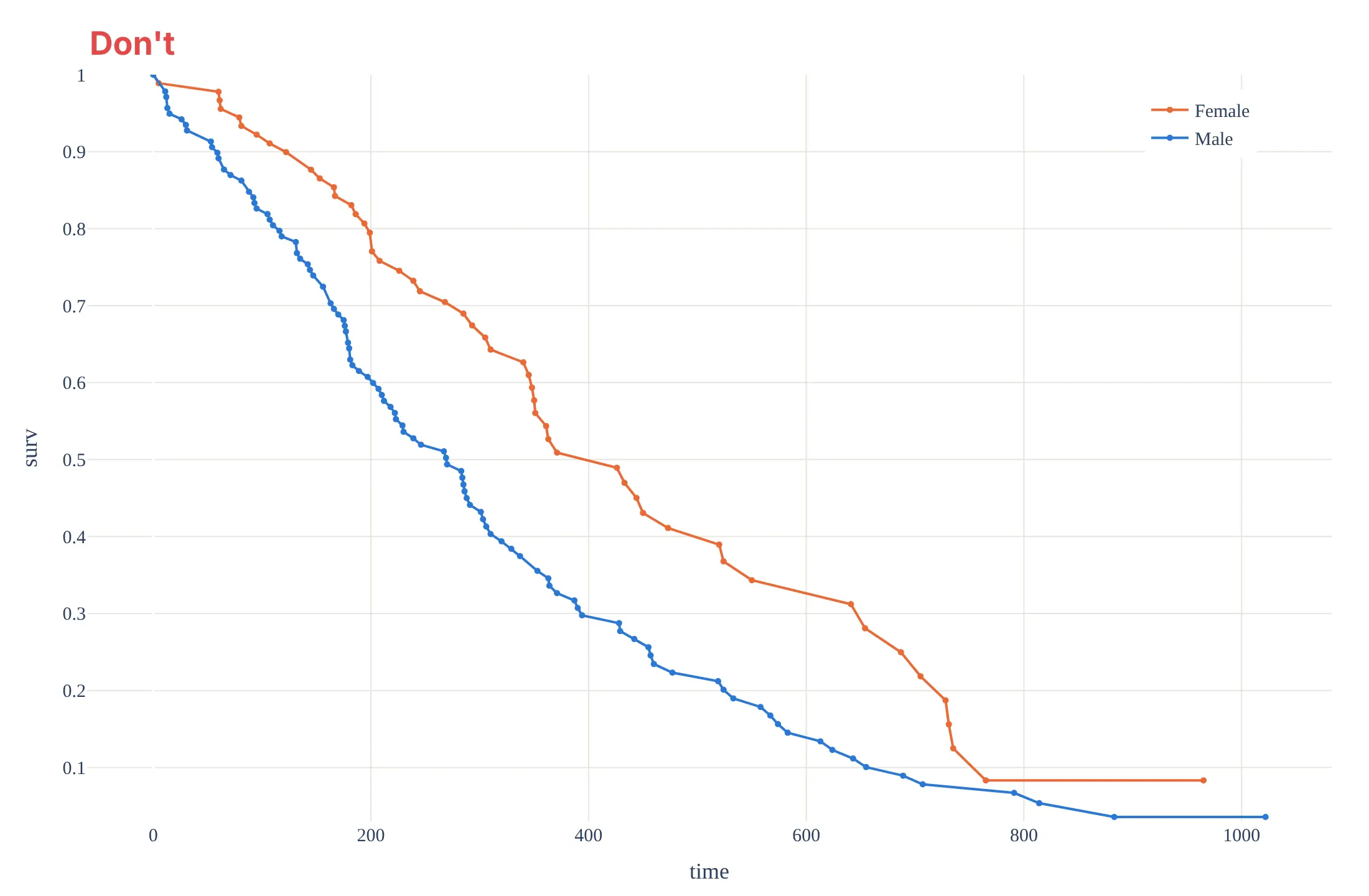
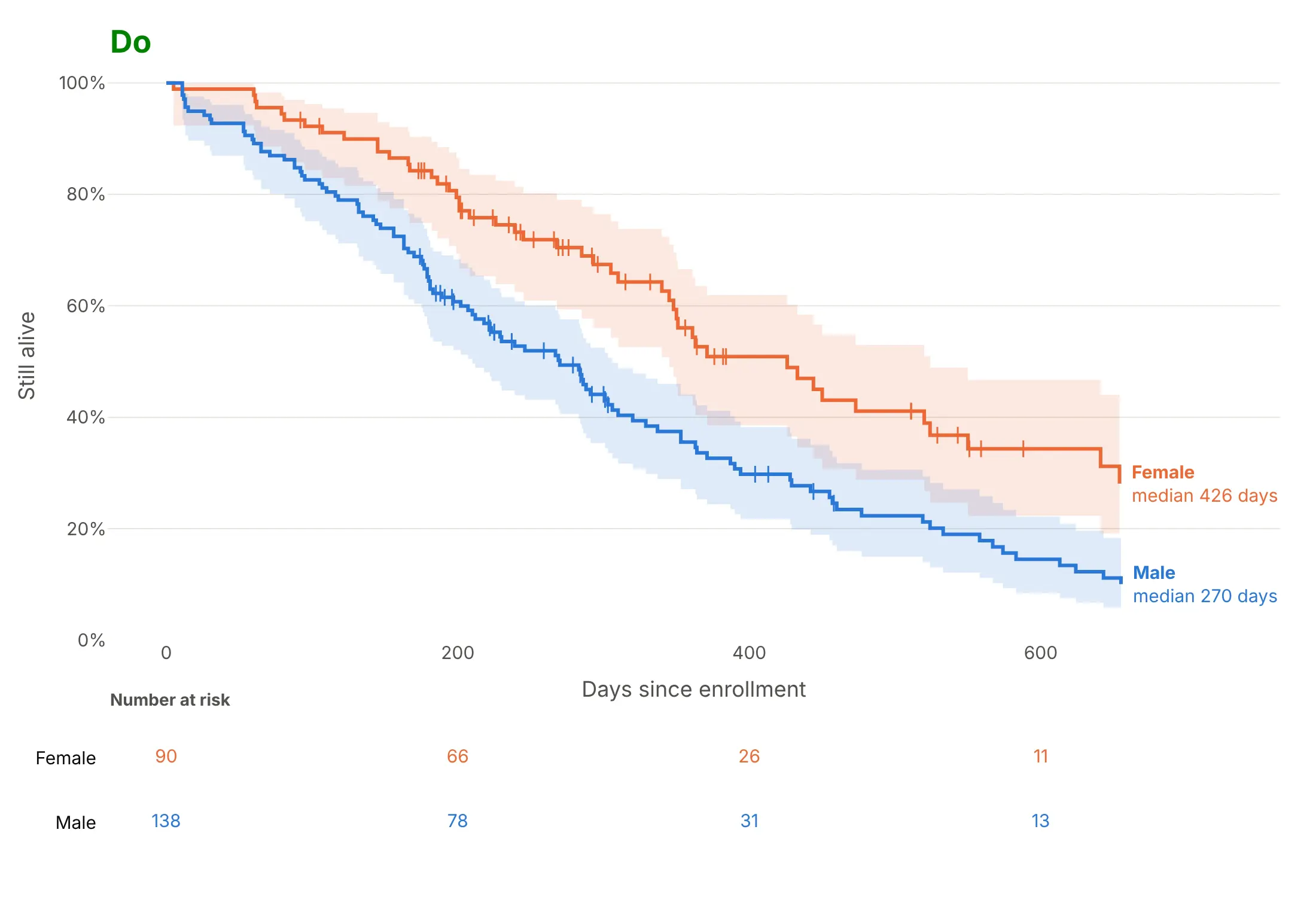
A survival curve is easy to draw wrong in ways that change what it says. Here is the same lung cancer data both ways, in the same colors.

Don't join the event times with straight lines, leave out the censored patients, run the curves out to the last two patients, or cut the y axis above zero with raw decimals:

The lung cancer survival curves drawn with mistakes: points joined by sloping lines with a marker at every death, no censoring marks, curves running to 1,022 days where only two patients remain, a y axis from 0.03 to 1 in decimals and a serif font

Do draw steps, mark censoring, show the uncertainty, stop where few remain and say how many are at risk:

The same curves as steps with censoring ticks, 95% confidence bands, a 0 to 100% axis, direct labels with the medians of 426 days for women and 270 for men, curves stopped at about 655 days when fewer than 10 patients remain, and a number-at-risk table underneath

Pick the style for the question

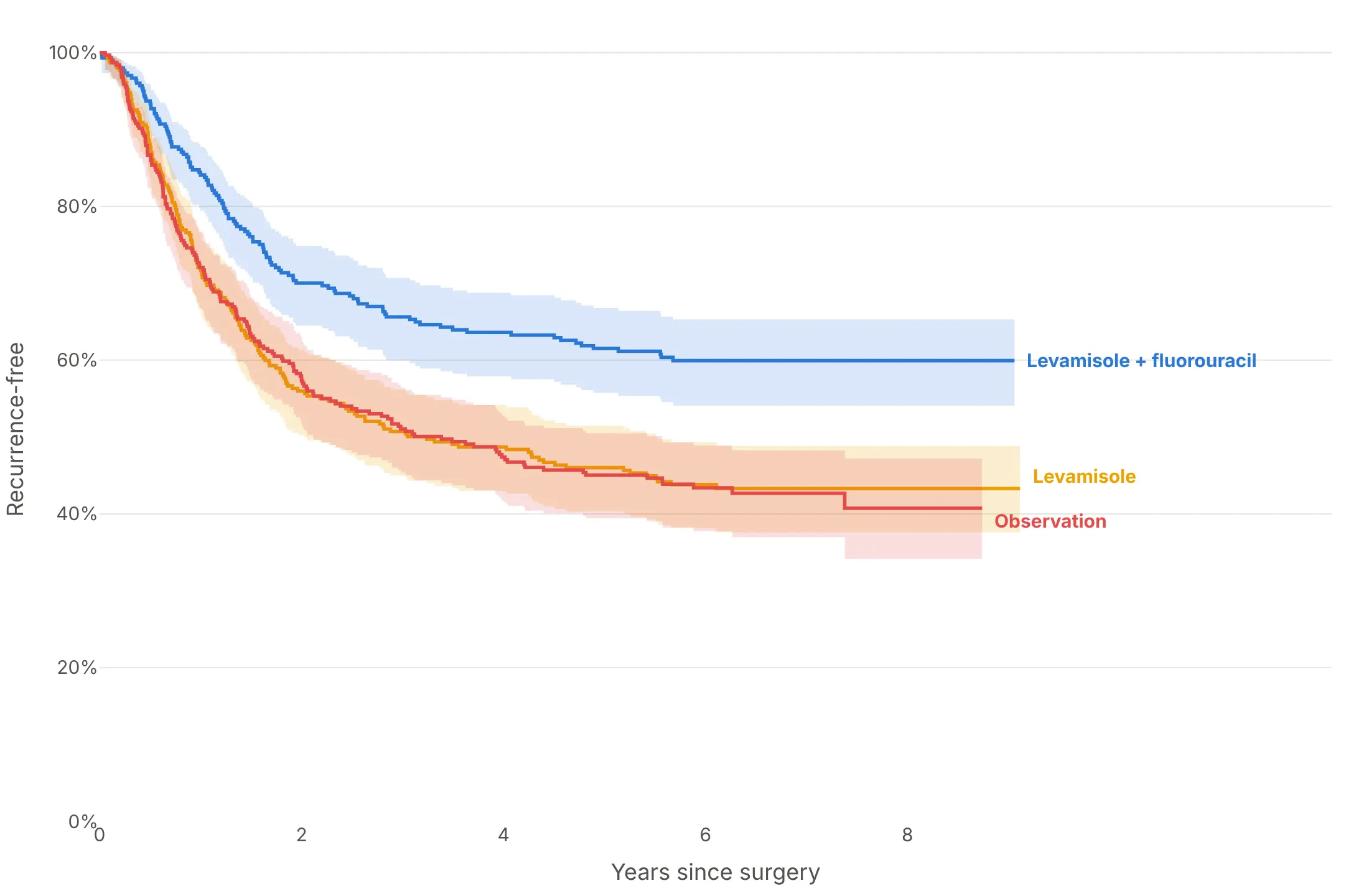
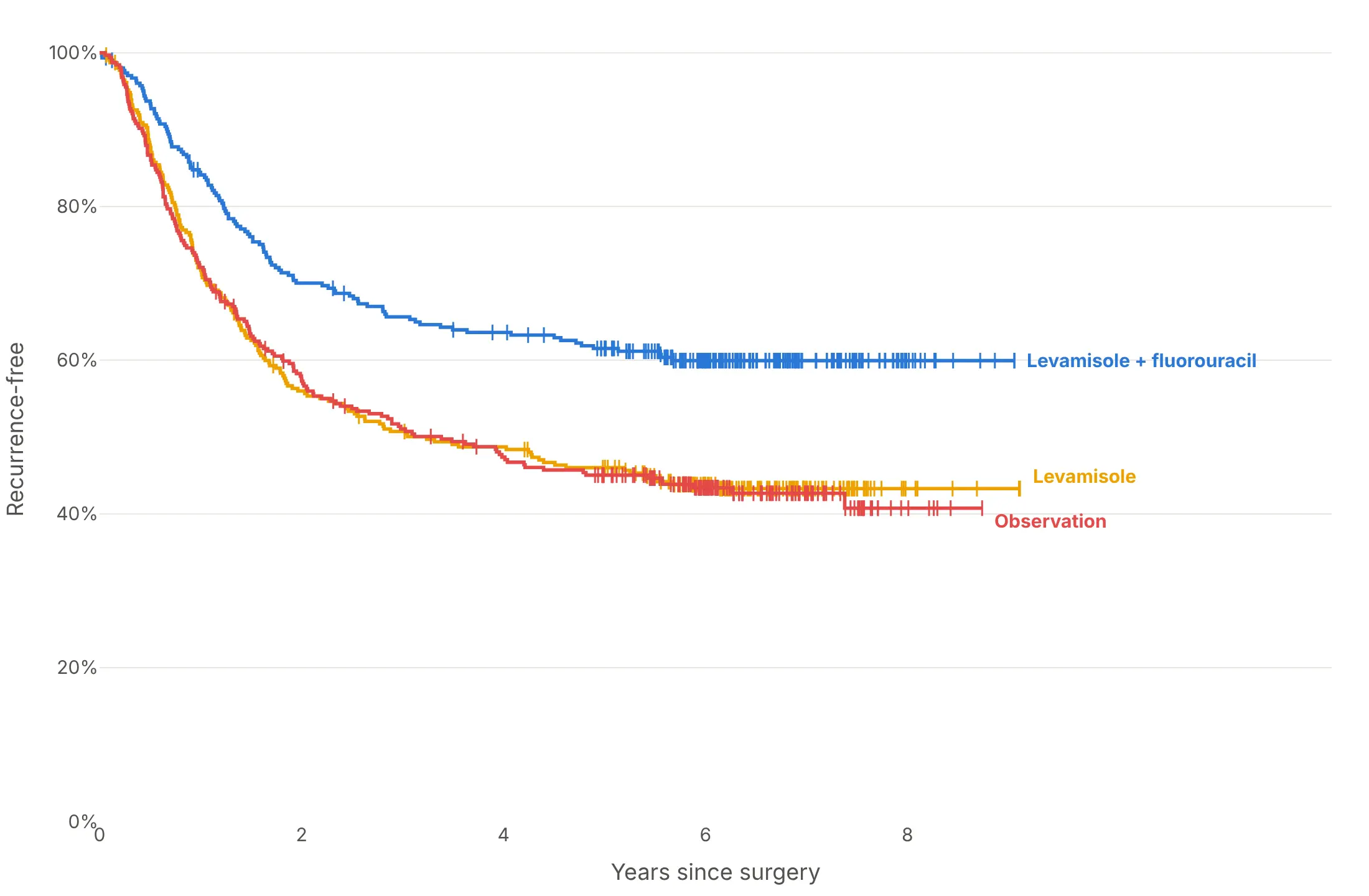
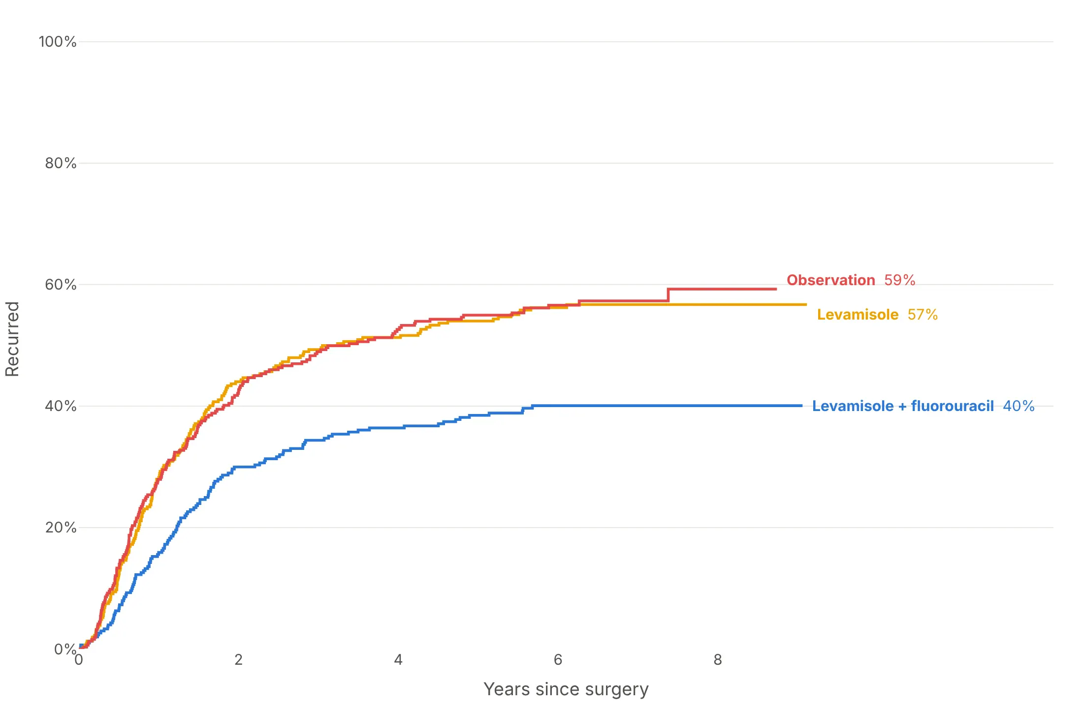
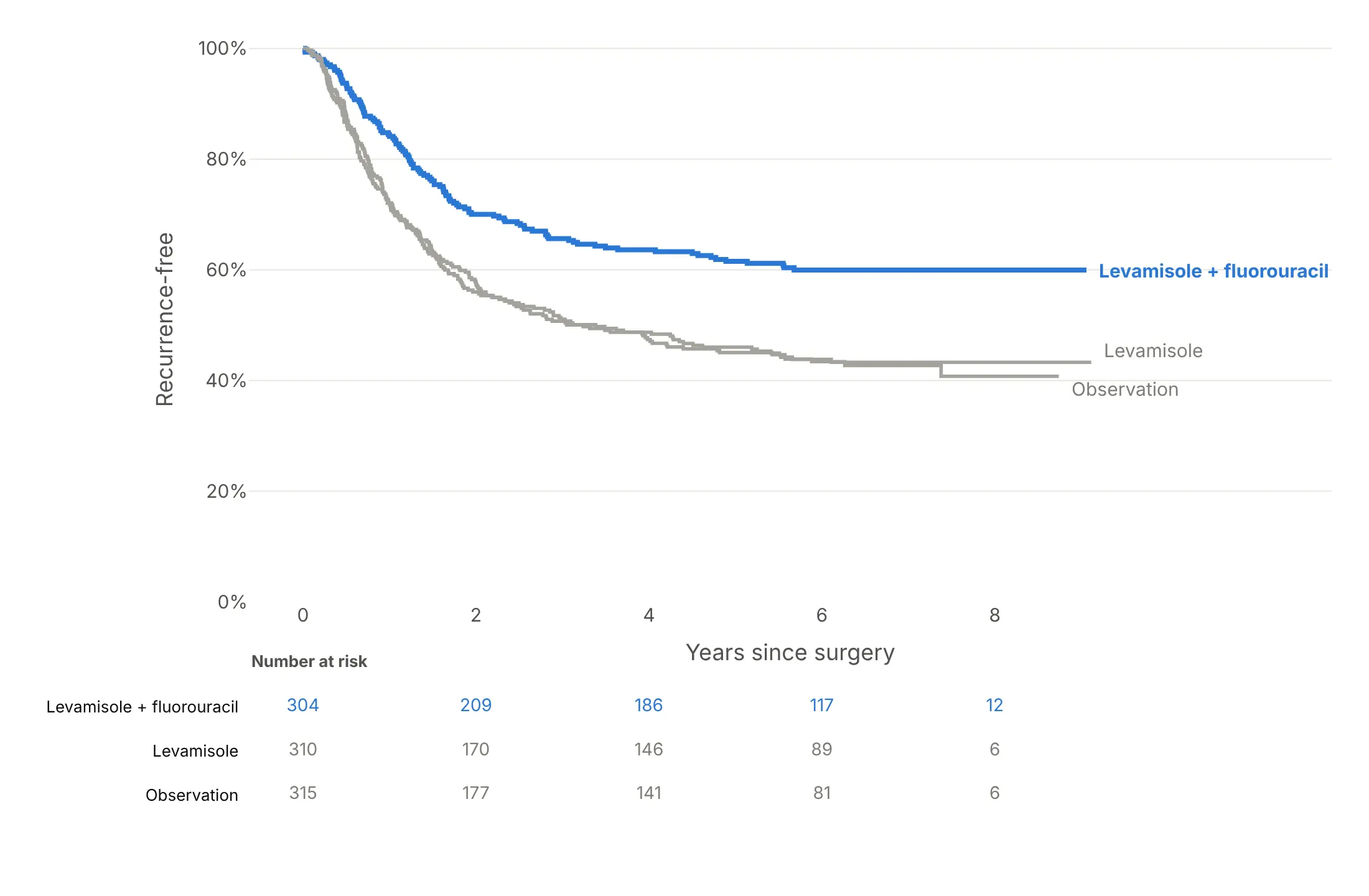
Here are four ways to style the colon cancer trial's three arms, each answering a different question.

Confidence bands. Show whether the gap between curves is bigger than the noise; here the treatment arm's band clears the other two from about year one.

Recurrence-free curves for three colon cancer trial arms with shaded 95% confidence bands: the levamisole plus fluorouracil band stays above the overlapping bands of the other two arms

Censoring ticks and direct labels. Show who is still being followed; the dense ticks after five years are patients whose follow-up ended without a recurrence.

The same three curves with a tick for every censored patient, dense from year five on, and the arm names at the end of each curve

Flipped to cumulative incidence. Count events instead of survivors: 40% of the treatment arm had recurred by the end of follow-up, against 59% with observation.

The three arms drawn as rising curves of the share who had a recurrence, ending at 40% for levamisole plus fluorouracil, 57% for levamisole and 59% for observation

One arm highlighted, with numbers at risk. The result for a slide: the treatment in color, the controls in gray and the table that says how much data is left.

The treatment arm in blue and the two control arms in gray, with a number-at-risk table falling from 304, 310 and 315 patients to 12, 6 and 6 at year eight

Checklist

Draw steps (line_shape="hv") that start at 100% at time zero.
Mark censored subjects with ticks, or say in the subtitle how many were censored.
Add 95% confidence bands, or at least confidence intervals for the numbers you quote.
Stop curves, or turn them dotted, when fewer than 10 to 20 subjects are at risk.
Add a number-at-risk table, and quote medians and landmark values from the curve.
Label curves directly and state the takeaway in the title.

Don't

Connect event times with sloping lines, which suggests events happened in between.
Drop censored subjects or count them as events.
Use 1 - KM for an event when a competing event can happen first; use cumulative incidence.
Compare curves that cross with a single hazard ratio or a single p-value without showing them.
Start the y axis above zero without saying so.

Options to customize

These are the go.Scatter and layout options that build a Kaplan-Meier curve. The full list is in the Plotly scatter reference.

line.shape="hv": draws a step that holds each value until the next event time, which is what the estimator means.
fill="tonexty": fills between this trace and the previous one; draw the lower bound, then the upper bound with the fill, for a confidence band.
fillcolor: a light tint such as rgba(42,120,214,0.15) or "#2a78d633", so bands overlap without hiding each other.
marker.symbol="line-ns-open": a short vertical tick for each censored subject, placed at the curve's value at that time.
mode="lines+markers": markers on every step, useful when time is discrete (seasons, cycles, visits).
make_subplots(rows=2, shared_xaxes=True, row_heights=[0.8, 0.2]): a number-at-risk table in the second row, as mode="text" traces.
yaxis.tickformat=".0%", range=[0, 1.02]: a 0-100% axis.
xaxis.type="log": for times that run from minutes to months (example in "What is").
fig.add_shape and fig.add_annotation: median drop lines, landmark lines at 1 or 5 years, and direct labels.
line.dash: dotted tails where few subjects remain, or a dashed reference curve.
hovertemplate, customdata: the number at risk and the survival estimate on hover.
showlegend=False on band and tick traces, so the legend lists only the groups.

More Kaplan-Meier curve examples

Nine more Kaplan-Meier curves built from real public data, each with its source, the technique that makes it work and a prompt to rebuild it.

1. The VA lung cancer trial: treatment vs cell type

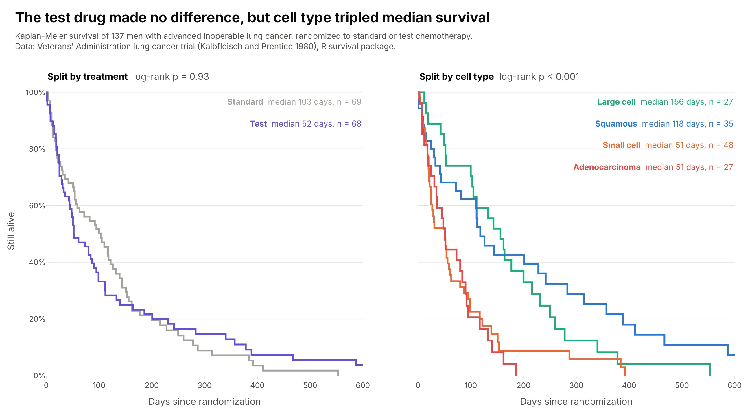
Two panels of Kaplan-Meier curves for 137 men with lung cancer. Split by treatment, the standard and test curves cross and the log-rank p is 0.93. Split by cell type, large cell (median 156 days) and squamous (118) separate from small cell and adenocarcinoma (51 days each), log-rank p < 0.001

Split by treatment, the curves cross and the log-rank test finds nothing (p = 0.93). Split by tumor cell type, they separate within weeks: large-cell patients lived a median 156 days, small-cell and adenocarcinoma patients 51. Data: Veterans' Administration lung cancer trial (Kalbfleisch and Prentice), the veteran dataset in R's survival package.

Tip: two panels with make_subplots(cols=2, shared_yaxes=True) show a null split and a strong one on the same patients.

Get the data from the Veterans' Administration lung cancer trial (the veteran dataset in R's survival package,
Kalbfleisch and Prentice) and shape it into a table
(columns: time in days, event 1 = died 0 = censored, trt Standard/Test, celltype, karno).

Build a plotly figure with two Kaplan-Meier panels sharing the y axis: left split by trt, right by celltype.
- Step lines (line_shape="hv"), no bands; label each curve with its median and n in the panel corner.
- Log-rank p-value above each panel. Days on the x axis up to 600, y axis 0-100%.

2. Bilirubin and survival in primary biliary cholangitis

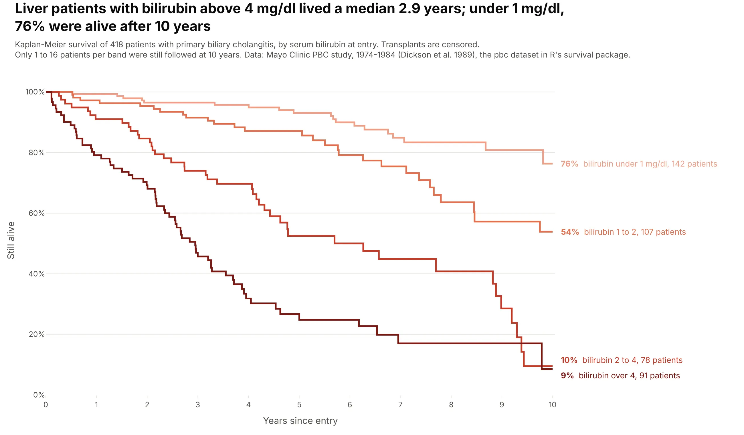
Kaplan-Meier survival over 10 years for 418 patients with primary biliary cholangitis in four bilirubin bands, light to dark red: 76% alive at 10 years under 1 mg/dl, 54% for 1 to 2, 10% for 2 to 4 and 9% over 4 mg/dl

Each step up in bilirubin at entry moves the curve down: 76% of patients under 1 mg/dl were alive after 10 years, and those over 4 mg/dl lived a median 2.9 years. Only 1 to 16 patients per band were still followed at 10 years. Data: Mayo Clinic PBC study, 1974-1984 (Dickson et al. 1989), the pbc dataset in R's survival package.

Tip: split a continuous risk factor into ordered bands and give them a sequential palette, so the order of the curves reads as a dose-response.

Get the data from the Mayo Clinic primary biliary cholangitis study (the pbc dataset in R's survival package)
and shape it into a table (columns: time in days, status 0 = censored 1 = transplant 2 = died, trt, bili in mg/dl, age).

Build plotly Kaplan-Meier curves of death (transplant censored) for bilirubin bands <1, 1-2, 2-4 and >4 mg/dl.
- Sequential reds from light to dark; years on the x axis, curves cut at 10 years.
- Labels in the right margin with each band's 10-year survival and n. Say in the subtitle how few are followed at 10 years.

3. Five-year survival for 33 cancers

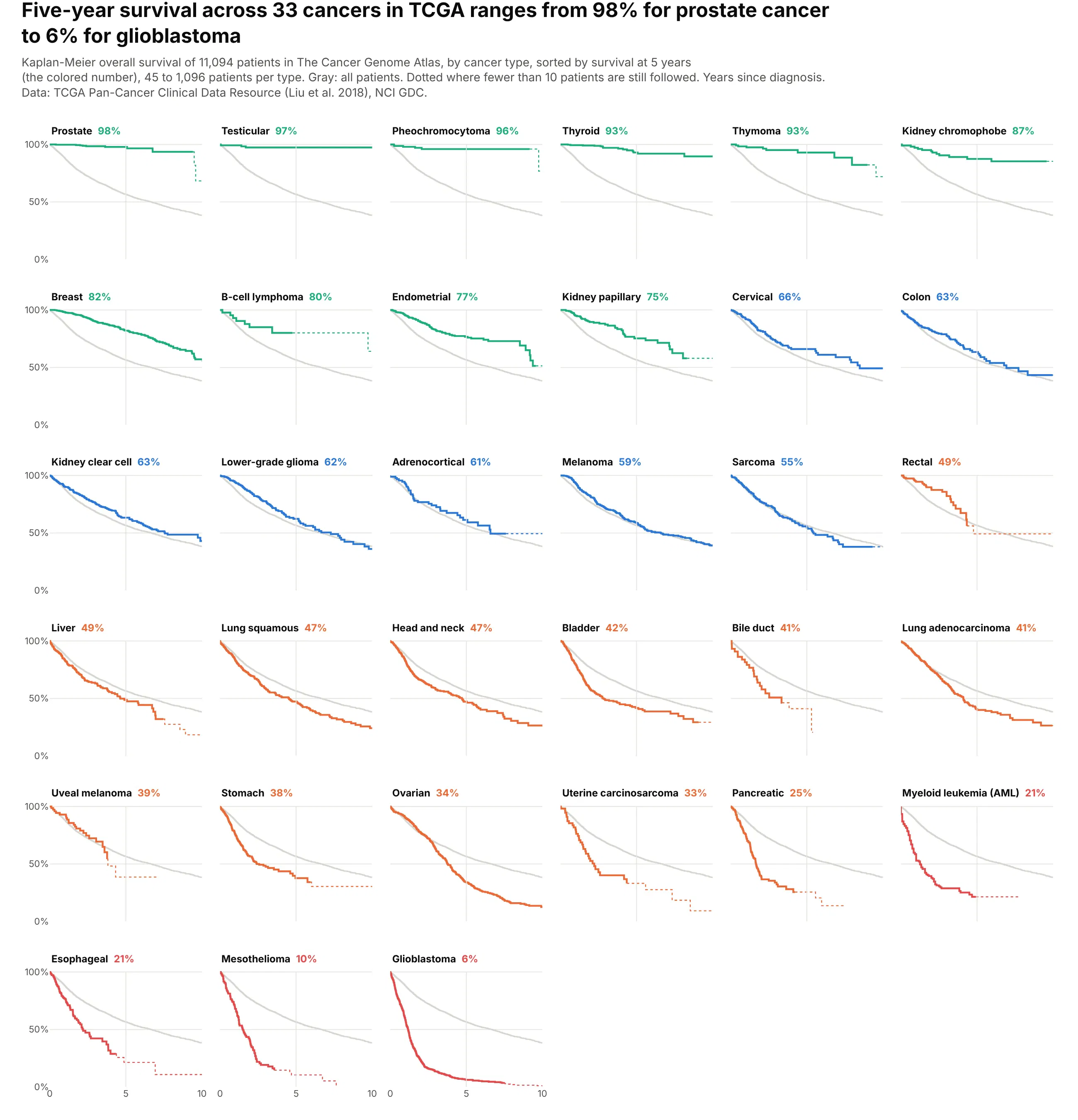
Small multiples of Kaplan-Meier overall survival for 33 cancer types in TCGA, sorted by 5-year survival from prostate (98%) and testicular (97%) to mesothelioma (10%) and glioblastoma (6%), each panel with the curve for all 11,094 patients in gray behind it and dotted tails where fewer than 10 patients remain

Across 11,094 patients in The Cancer Genome Atlas, five-year survival runs from 98% for prostate cancer to 6% for glioblastoma. Sorting 33 small panels by that number turns them into a ranked table that still shows each curve's shape. Data: TCGA Pan-Cancer Clinical Data Resource (Liu et al. 2018), NCI Genomic Data Commons.

Tip: draw the curve for everyone in light gray behind every panel, so each cancer is compared with the same reference.

Get the data from the TCGA Pan-Cancer Clinical Data Resource (Liu et al. 2018, Table S1 on the NCI GDC)
and shape it into a table (columns: type, time = OS.time in days, event = OS, stage).

Build a plotly grid of small multiples (6 columns) with one Kaplan-Meier curve per cancer type, sorted by 5-year survival.
- Behind every panel, the curve of all patients in light gray. Years on the x axis, 0 to 10.
- Solid while at least 10 patients are at risk, dotted after. Panel title: type name and 5-year survival.

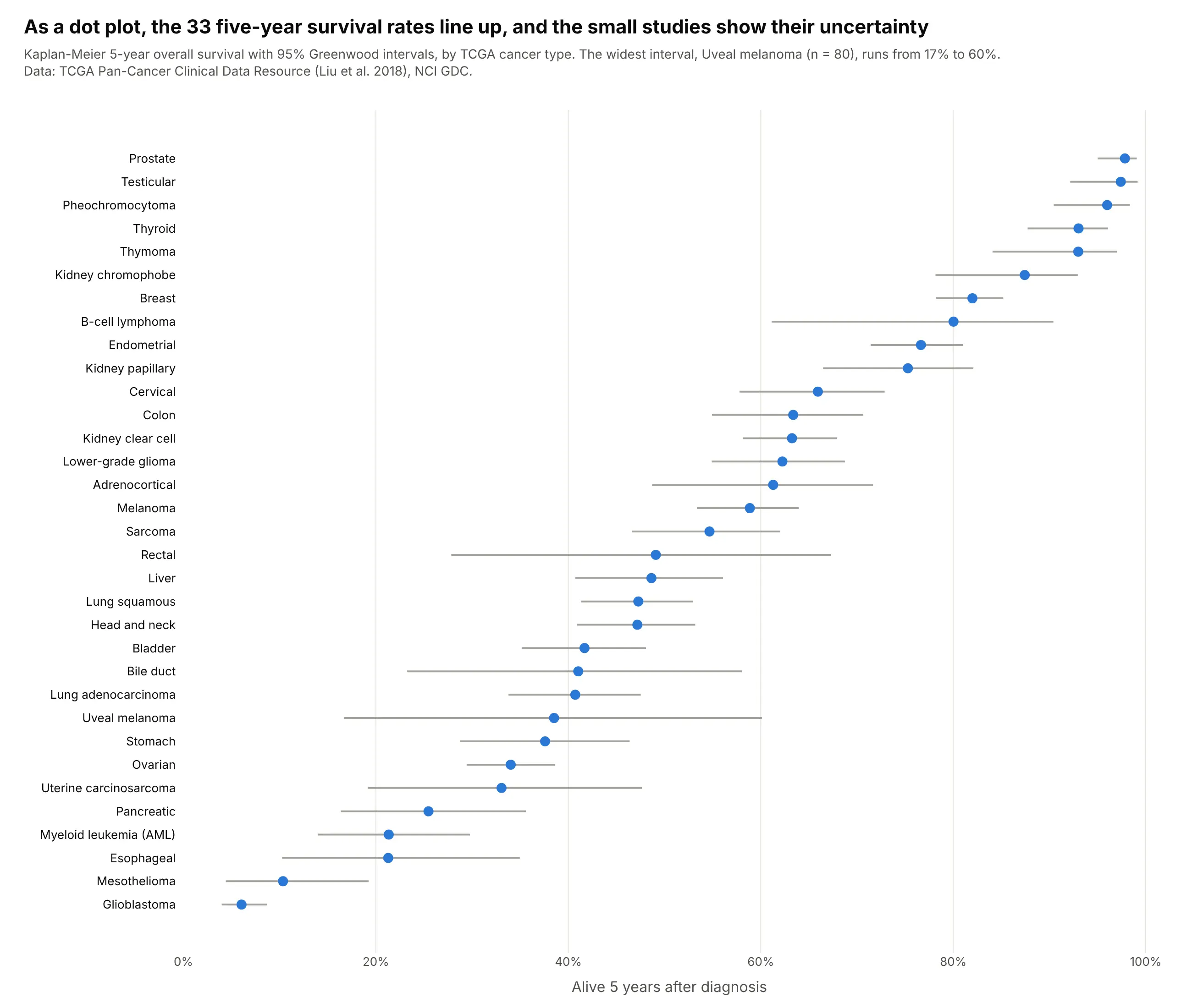
Another way to see it: a dot plot of the 33 five-year rates with their 95% intervals is easier to rank and shows the uncertainty of the small studies, such as uveal melanoma (n = 80, 17% to 60%).

Dot plot of 5-year overall survival with 95% confidence intervals for 33 TCGA cancer types, from prostate at 98% to glioblastoma at 6%; the widest interval is uveal melanoma, 17% to 60%

4. How long US trials take to report their results

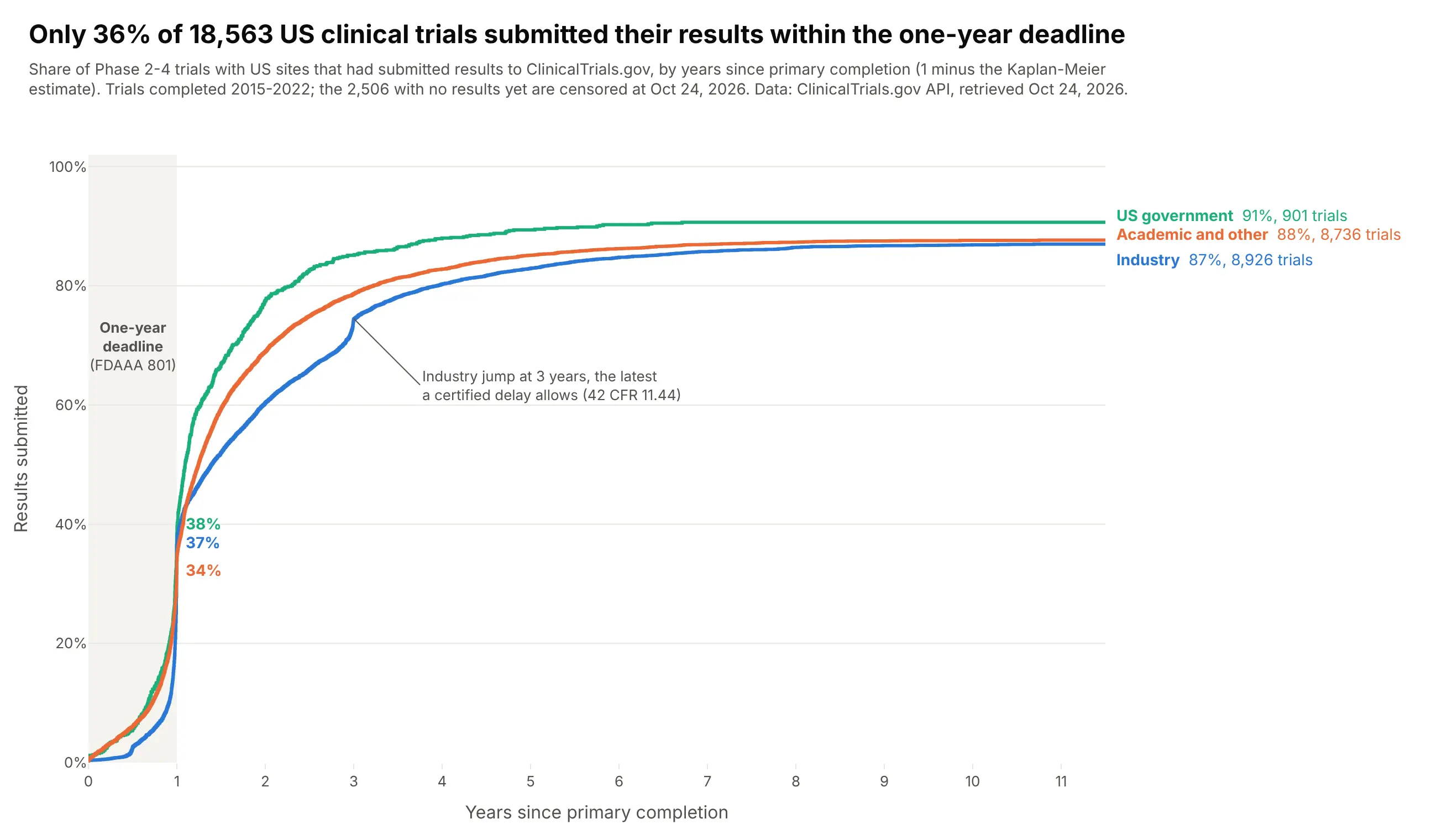
Rising curves of the share of 18,563 US Phase 2-4 trials that had submitted results to ClinicalTrials.gov, by years since primary completion. 38% of US government trials, 37% of industry trials and 34% of academic trials had reported by the one-year deadline; industry jumps at 3 years, and the curves level off at 91%, 87% and 88%

Only 36% of 18,563 US Phase 2-4 trials completed in 2015-2022 had submitted results within a year of primary completion, the deadline under FDAAA. Industry trials jump at three years, the latest a certified delay allows, and 2,506 trials still had nothing posted in October 2026. Data: ClinicalTrials.gov API v2.

Tip: when the event is good news, plot 1 - KM so the curve rises, and shade the deadline.

Get the data from the ClinicalTrials.gov API v2: interventional Phase 2-4 trials with a US site, completed or terminated,
primary completion 2015-2022, and shape it into a table
(columns: nct, sponsor class, phase, primary_completion, time = days to the first results submission, event = 1 if submitted).
Trials without results are censored at today.

Build plotly cumulative incidence curves (1 minus Kaplan-Meier) by sponsor class, in years.
- Shade the first year and label each curve's value at 1 year; end labels with the final share and n.
- Annotate the jump at 3 years (certified delay). Title with the overall share reported within 1 year.

5. What happens to new banks: failure or merger

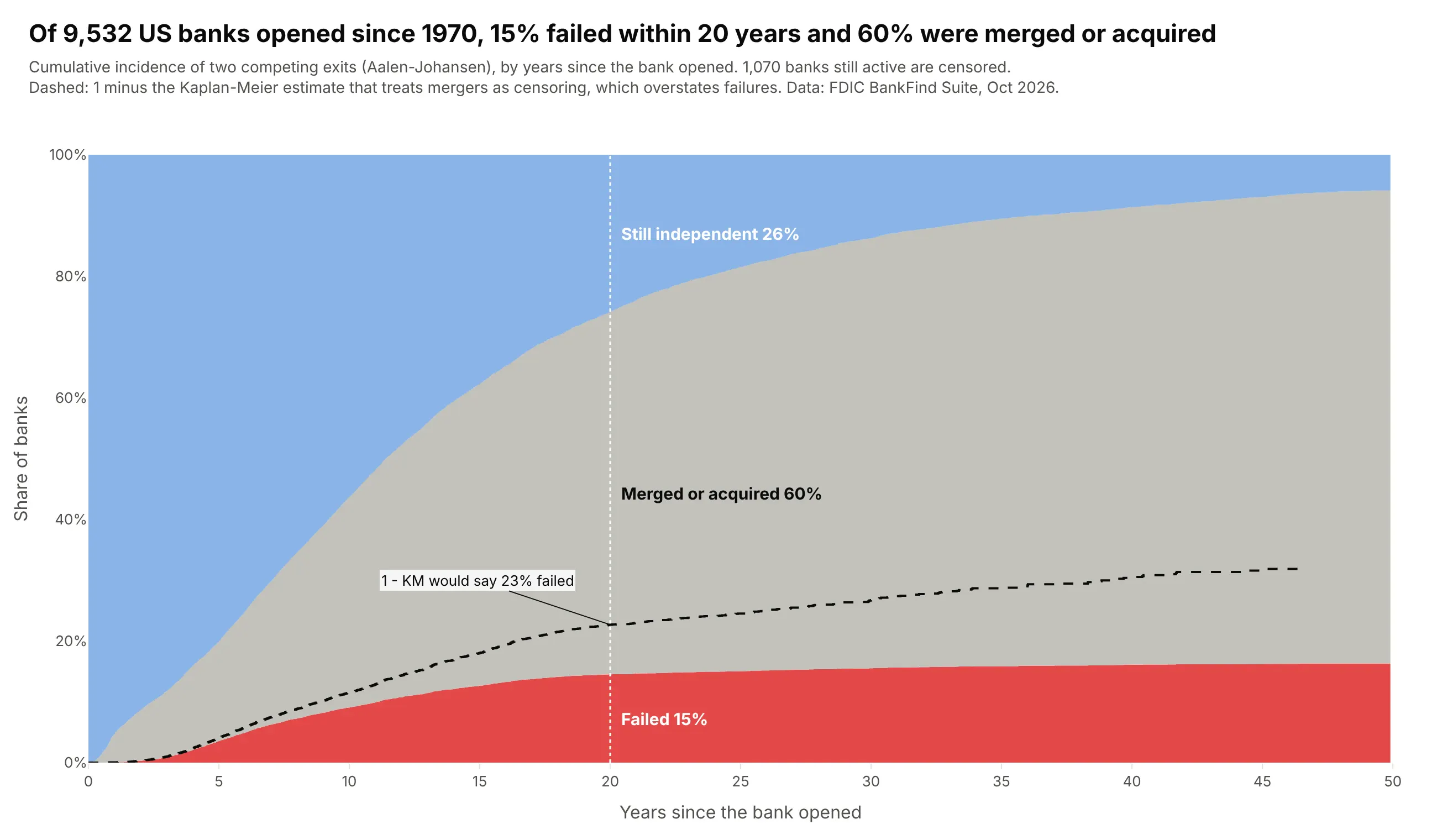
Stacked areas of the share of 9,532 US banks opened since 1970 that failed, were merged or acquired, or are still independent, by years since opening. At 20 years, 15% had failed, 60% had merged and 26% were still independent; a dashed 1 minus Kaplan-Meier line overstates failures at 23%

Of 9,532 US banks opened since 1970, 15% failed within 20 years and 60% were merged or acquired. Treating mergers as censoring, the naive 1 - KM line, would say 23% failed. Data: FDIC BankFind Suite (institutions and failures).

Tip: with competing exits, stack the Aalen-Johansen cumulative incidences with fill="tonexty" so the states add up to 100%.

Get the data from the FDIC BankFind Suite API (institutions with established and end dates, and the failures list)
and shape it into a table (columns: cert, established, years since opening, outcome = active/merged/failed).
Keep banks established since 1970; active banks are censored.

Build a plotly stacked step-area chart of cumulative incidence (Aalen-Johansen) of failure and of merger,
with "still independent" on top, over 50 years.
- Add 1 - Kaplan-Meier for failure (mergers censored) as a dashed line to show the bias.
- Label the three shares at 20 years inside the areas.

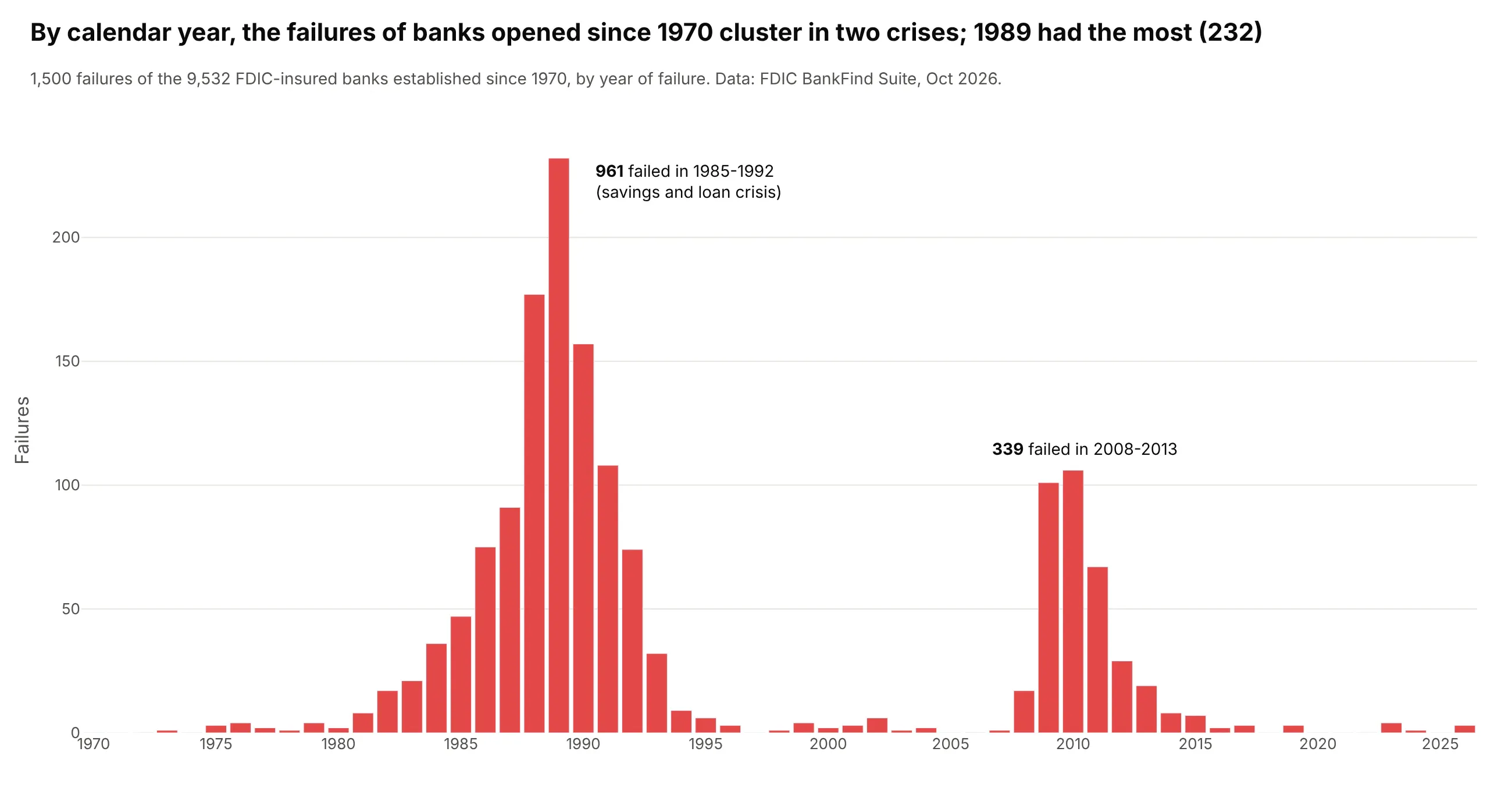
Another way to see it: a bar chart of failures by calendar year shows when they happened, 961 in 1985-1992 and 339 in 2008-2013, which the time-since-opening axis hides.

Bar chart of failures of banks opened since 1970 by calendar year, with 961 failures in 1985-1992 peaking at 232 in 1989, and 339 in 2008-2013

6. How long Apache Spark bugs stay open

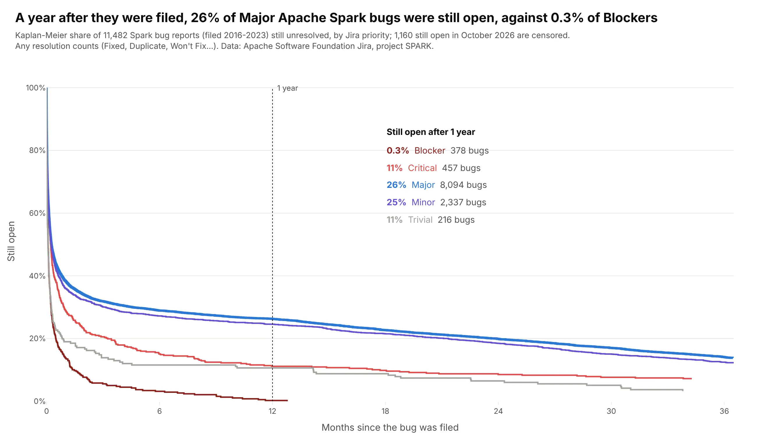
Kaplan-Meier curves of the share of 11,482 Apache Spark bug reports still open by months since filing, for five priorities. After a year 0.3% of Blockers, 11% of Critical, 26% of Major, 25% of Minor and 11% of Trivial bugs were still open

Half of all Spark bug reports were resolved within 7.3 days, but the curves flatten into a long tail: a year after filing, 26% of Major bugs were still open, against 0.3% of Blockers. Data: Apache Software Foundation Jira, project SPARK, bugs filed 2016-2023.

Tip: when labels at the curve ends would collide, list the values at one landmark in the empty corner of the plot.

Get the data from the Apache Software Foundation Jira REST API (project SPARK, issue type Bug, created 2016-2023)
and shape it into a table (columns: key, priority, resolution, days from created to resolved, event = 1 if resolved).
Unresolved tickets are censored at today.

Build plotly Kaplan-Meier curves of the share still open by priority, x in months up to 36.
- Thicker line for Major (the default priority); a dotted guide at 12 months.
- A small table in the top right with each priority's share still open at 1 year and its count.

7. How long Supreme Court justices serve

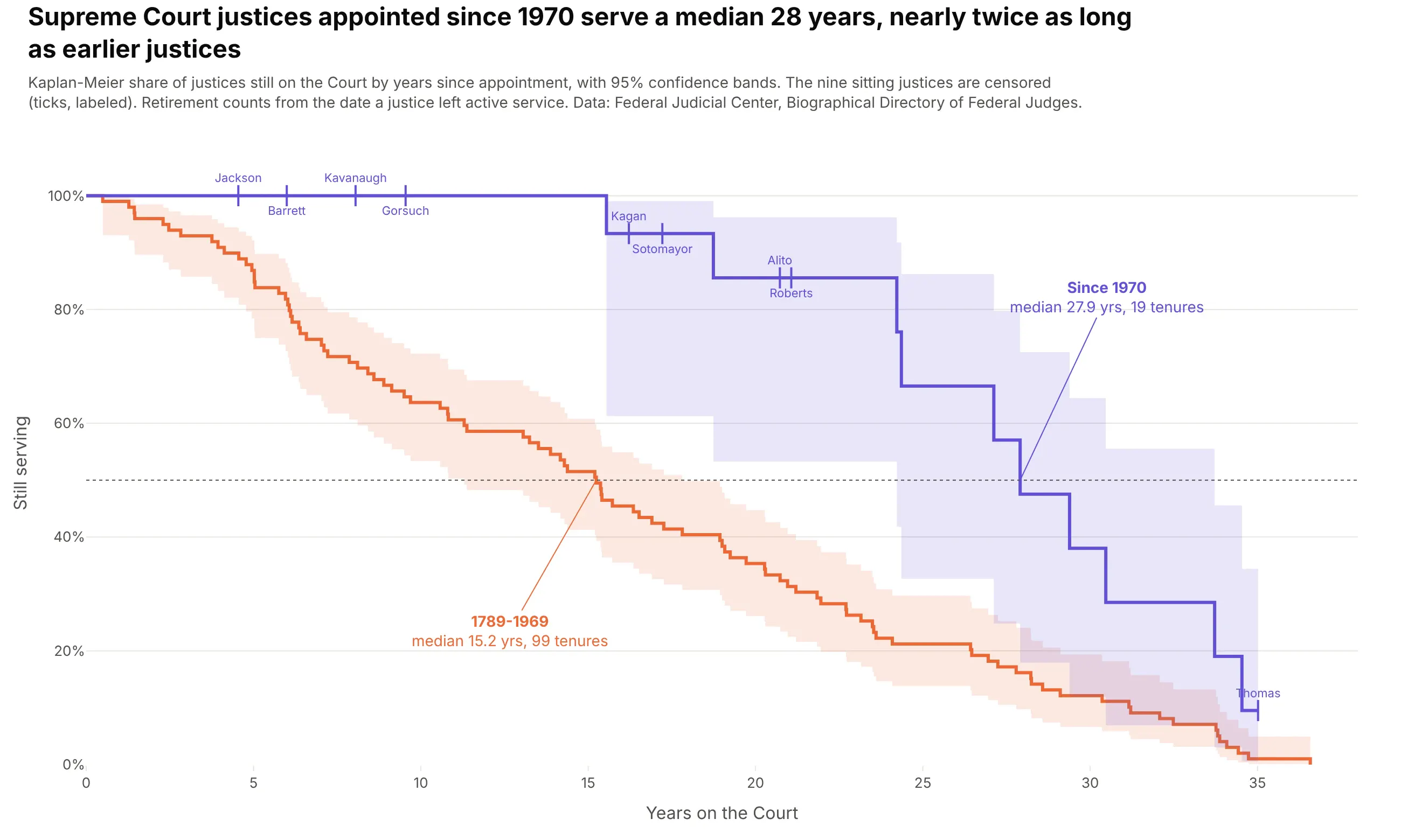
Kaplan-Meier curves of US Supreme Court justices still serving by years on the Court, with 95% bands. Justices appointed 1789-1969 (99 tenures) served a median 15.2 years; those appointed since 1970 (19 tenures) a median 27.9 years, with the nine sitting justices marked as censored ticks labeled with their names

Justices appointed since 1970 serve a median 28 years, against 15.2 for the 99 tenures before. Nine of those 19 justices are still serving, so averaging the finished tenures would understate it. Data: Federal Judicial Center, Biographical Directory of Article III Federal Judges.

Tip: label the censoring ticks with names when there are only a few; it shows exactly who the estimate is still waiting on.

Get the data from the Federal Judicial Center's Biographical Directory of Article III Federal Judges (judges.csv)
and shape it into a table of Supreme Court tenures (columns: justice, start, end, years, event = 1 if ended, termination).
Use the retirement (senior status) date as the end when present; sitting justices are censored.

Build plotly Kaplan-Meier curves for justices appointed before 1970 and since 1970, with 95% Greenwood bands.
- Censoring ticks labeled with the sitting justices' last names, alternating above and below the curve.
- Medians marked on the 50% line with callouts.

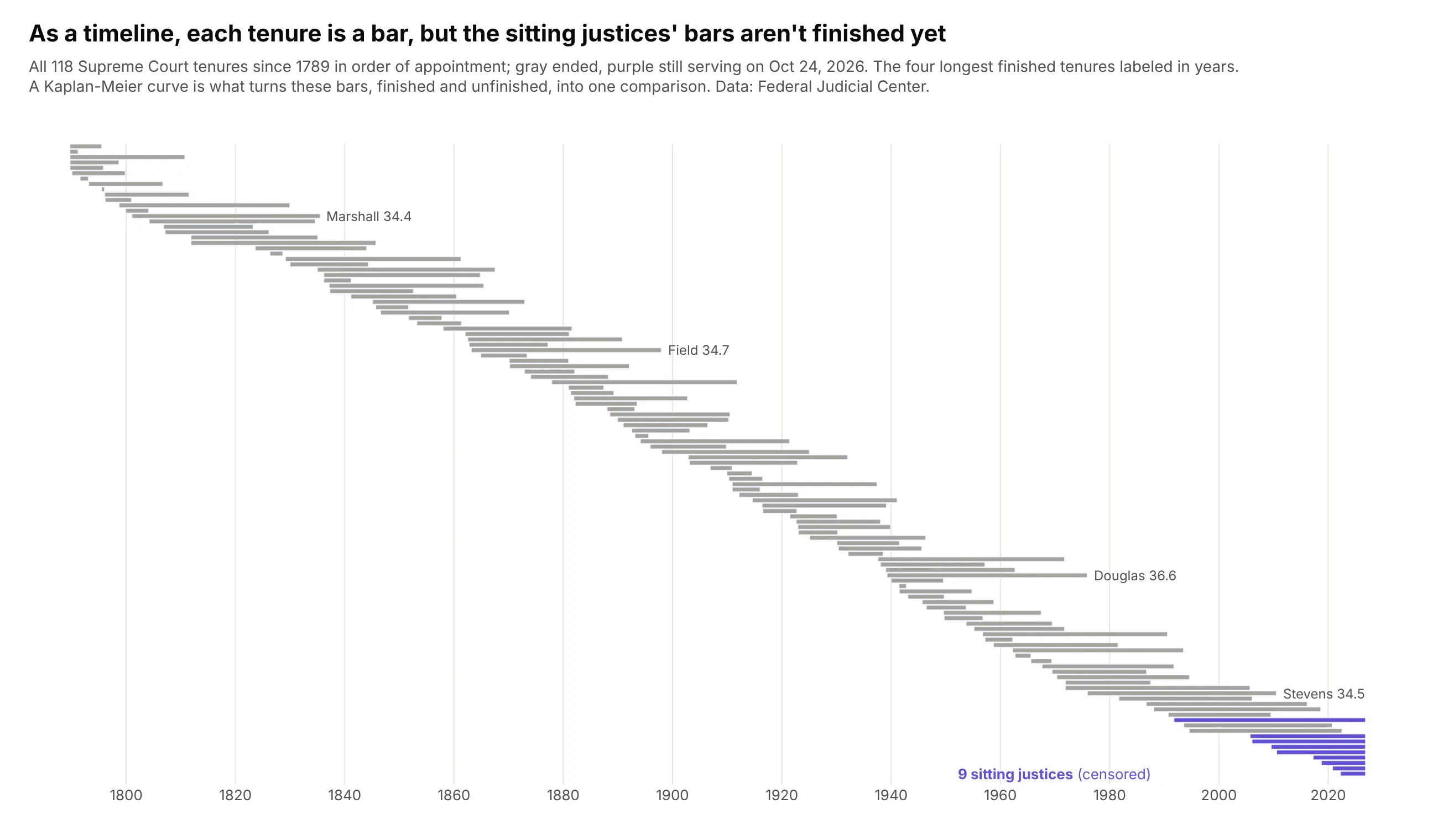
Another way to see it: a timeline of every tenure shows the history at a glance, but the nine unfinished bars can't be compared with the finished ones without a survival estimate.

Timeline of all 118 Supreme Court tenures since 1789 as horizontal bars in order of appointment, gray for finished and purple for the nine sitting justices, with Douglas (36.6 years), Field, Stevens and Marshall labeled

8. How long Starlink satellites stay in orbit

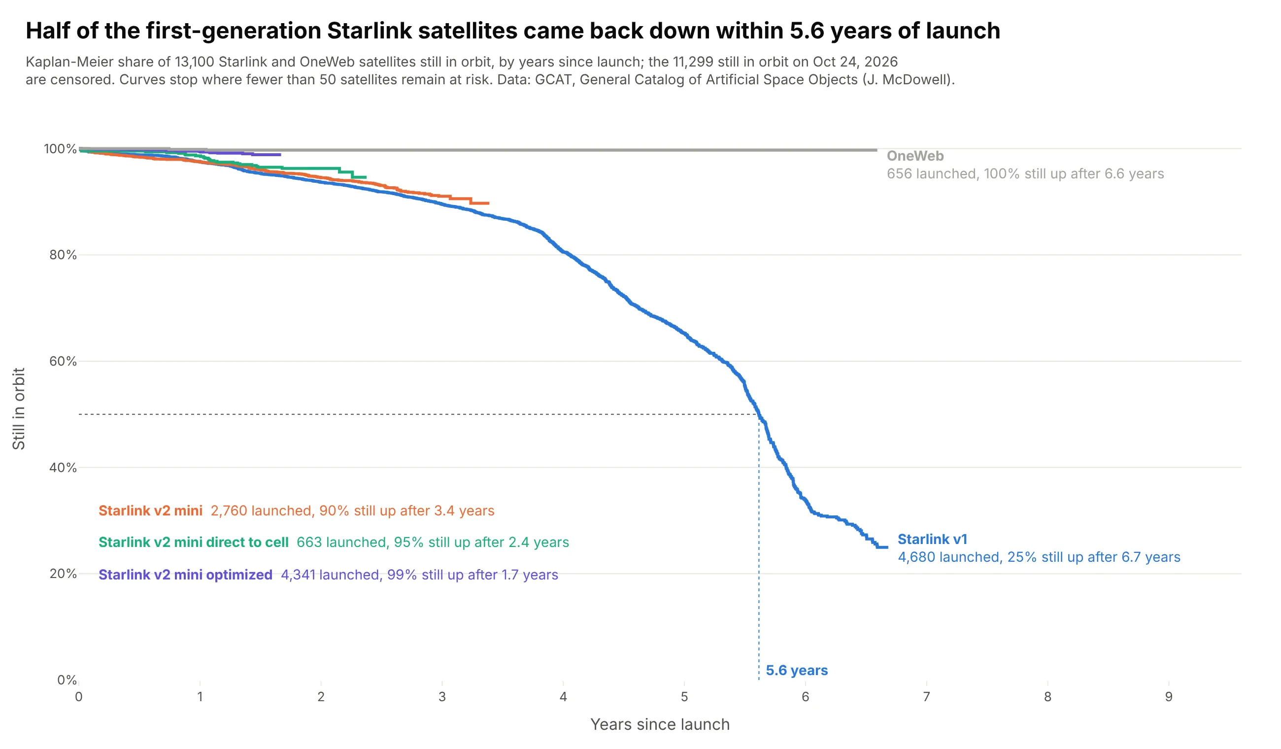
Kaplan-Meier curves of the share of 13,100 Starlink and OneWeb satellites still in orbit by years since launch. Half of the 4,680 first-generation Starlink satellites came down within 5.6 years; newer Starlink generations end early at 90% to 99% still up, and OneWeb is at 100% after 6.6 years

Half of the 4,680 first-generation Starlink satellites came back down within 5.6 years of launch. 11,299 of the 13,100 satellites are still up, so the newer generations' curves end early instead of guessing. Data: GCAT, General Catalog of Artificial Space Objects (Jonathan McDowell).

Tip: stop each curve where fewer than 50 subjects remain at risk, so groups with short follow-up don't drift on a handful of points.

Get the data from Jonathan McDowell's General Catalog of Artificial Space Objects (GCAT satcat.tsv)
and shape it into a table (columns: group = Starlink bus generation or OneWeb, launch, years in orbit, event = 1 if reentered).
Satellites still in orbit are censored at today.

Build plotly Kaplan-Meier curves of the share still in orbit by group, years since launch.
- Stop each curve when fewer than 50 satellites are at risk.
- Mark the median of Starlink v1 with dotted lines; list the newer generations' end values in a block of text.

9. How long MLB careers last

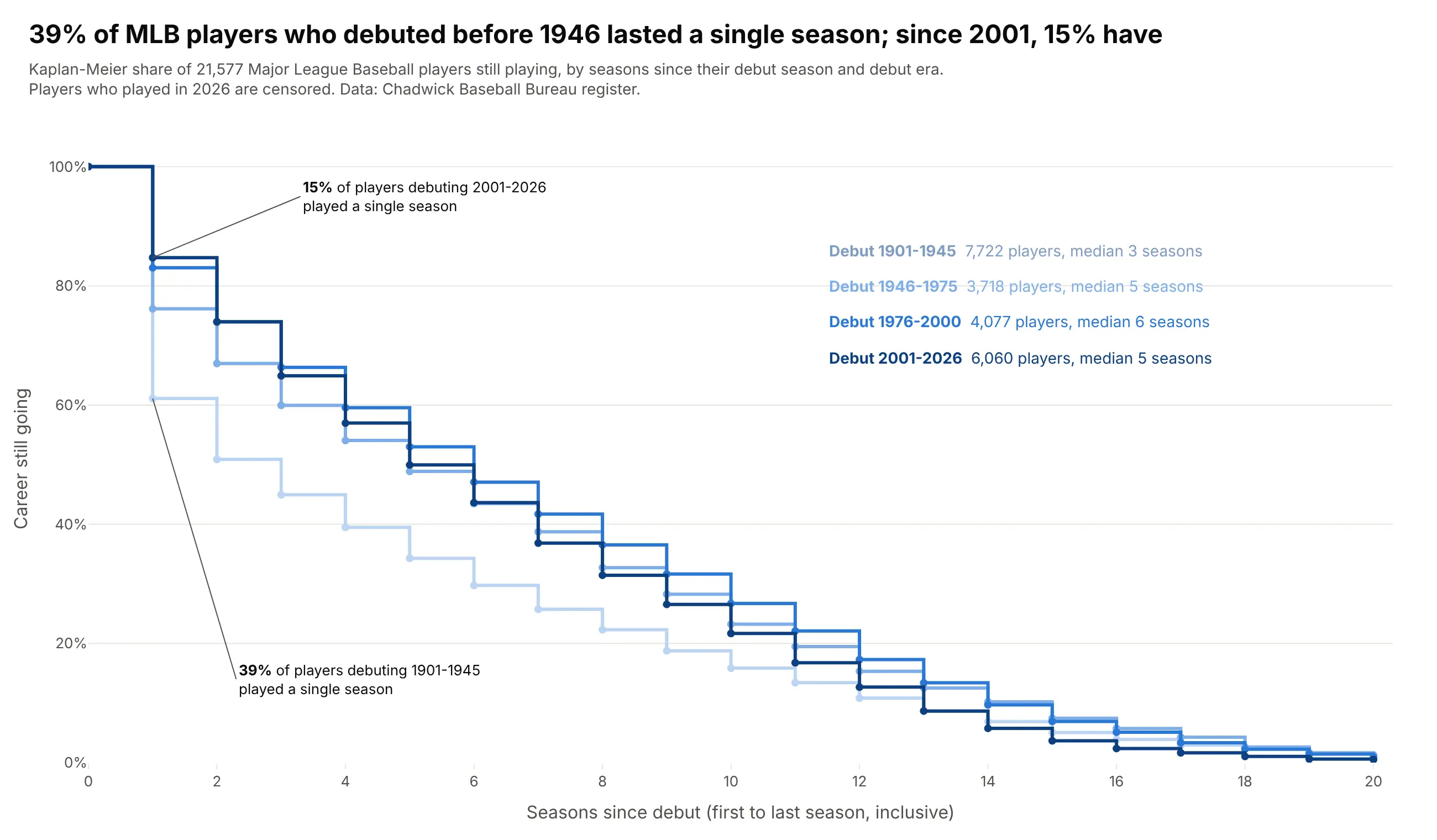
Kaplan-Meier curves of MLB careers by seasons since debut for four debut eras, drawn as steps with a dot per season. 39% of players who debuted 1901-1945 played a single season, against 15% since 2001; median careers were 3, 5, 6 and 5 seasons

39% of the 7,722 players who debuted in 1901-1945 played a single season in the majors; since 2001 it's 15%. The 1,472 players who played in 2026 are censored, since their careers may go on. Data: Chadwick Baseball Bureau register.

Tip: when time is counted in whole units, add a marker on each step (mode="lines+markers") so the values at 1, 2, 3 seasons are easy to read.

Get the data from the Chadwick Baseball Bureau register (people files, mlb_played_first and mlb_played_last)
and shape it into a table (columns: debut, seasons = last - first + 1, event = 0 if they played in the latest season, era).

Build plotly Kaplan-Meier curves of careers still going by seasons since debut for the eras 1901-1945, 1946-1975,
1976-2000 and 2001-2026, up to 20 seasons.
- Step lines with a dot per season, sequential blues from early to recent.
- Annotate the share who played a single season for the first and last era.