Step Charts - A Complete Guide

TL;DR

• A step chart draws a value that holds until it changes as flat steps joined by vertical jumps, so the chart shows the value on every date, not only on the days it was measured. Interest rates, prices, tariffs, tax brackets, counts, and inventory levels all behave like this.
• Step charts are also known as step line charts, step plots, and stairstep graphs (MATLAB’s stairs), and they draw what mathematicians call a step function. They are similar to line charts, which draw straight lines between points, and to step area charts, and the ECDF plot and the Kaplan-Meier curve are both step charts.
• In Plotly, a step chart is a line with line_shape="hv". Use "hv" when each date is the start of a value, "vh" when it’s the end, and "hvh" when it’s the middle, and add one last point at today’s date so the current value gets a step of its own.

What is a step chart?

Step charts look like this:

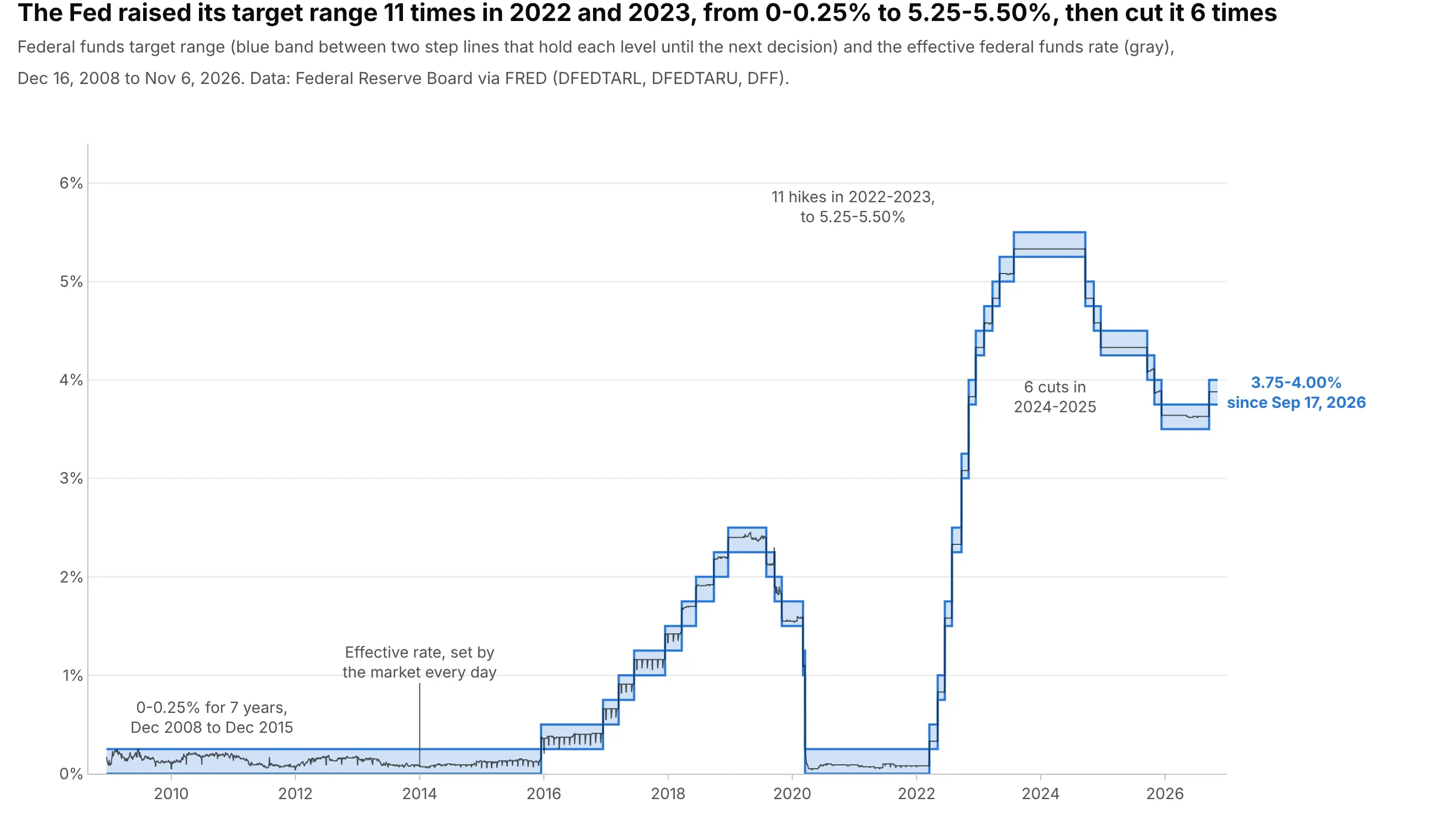
Data: Federal Reserve Board via FRED (Federal Reserve Economic Data; series DFEDTARL, DFEDTARU, and DFF).

How do you read a step chart? In the example above, notice these things:

• The blue band is the federal funds target range, the interest rate range the Federal Reserve (the Fed) sets for overnight loans between banks. It doesn’t change between decisions, so each flat stretch is a period when one range was in force, from 0% to 0.25% for seven years from December 2008 to December 2015, up to 5.25% to 5.50% from July 2023.
• Each vertical jump is one decision, drawn on the day it took effect. The 11 short steps up in 2022 and 2023 are 11 hikes, and the six steps down in 2024 and 2025 are six cuts.
• A flat line is a claim: on every day between two jumps, the range was exactly that level. That is why the chart uses steps and not a straight line between decisions, which would show rates in between that were never set.
• The thin gray line is the effective rate that banks actually paid each day, which moves with the market. It stayed inside the range on 6,527 of 6,534 days, so the gray line is ordinary data and the blue band is a step function around it.

It’s often used for charts like these:

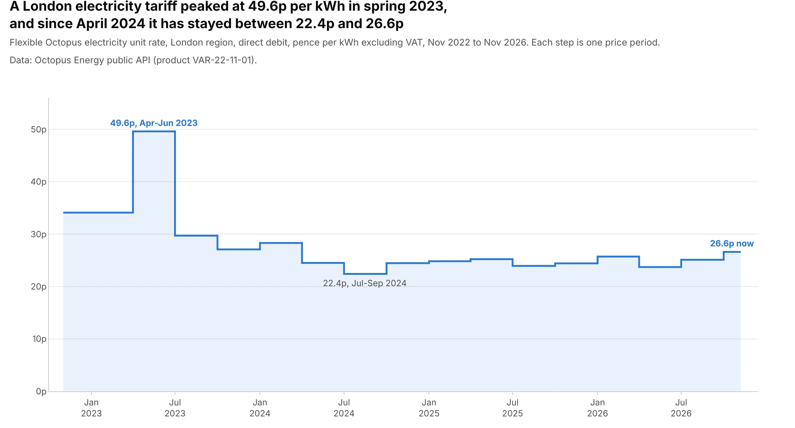
Prices and tariffs. A UK electricity tariff that changes with the energy regulator’s quarterly price cap peaked at 49.6p per kWh from April to June 2023 and has stayed between 22.4p and 26.6p since April 2024, one step per quarter. Data: Octopus Energy public API (Flexible Octopus, London region, excluding VAT).

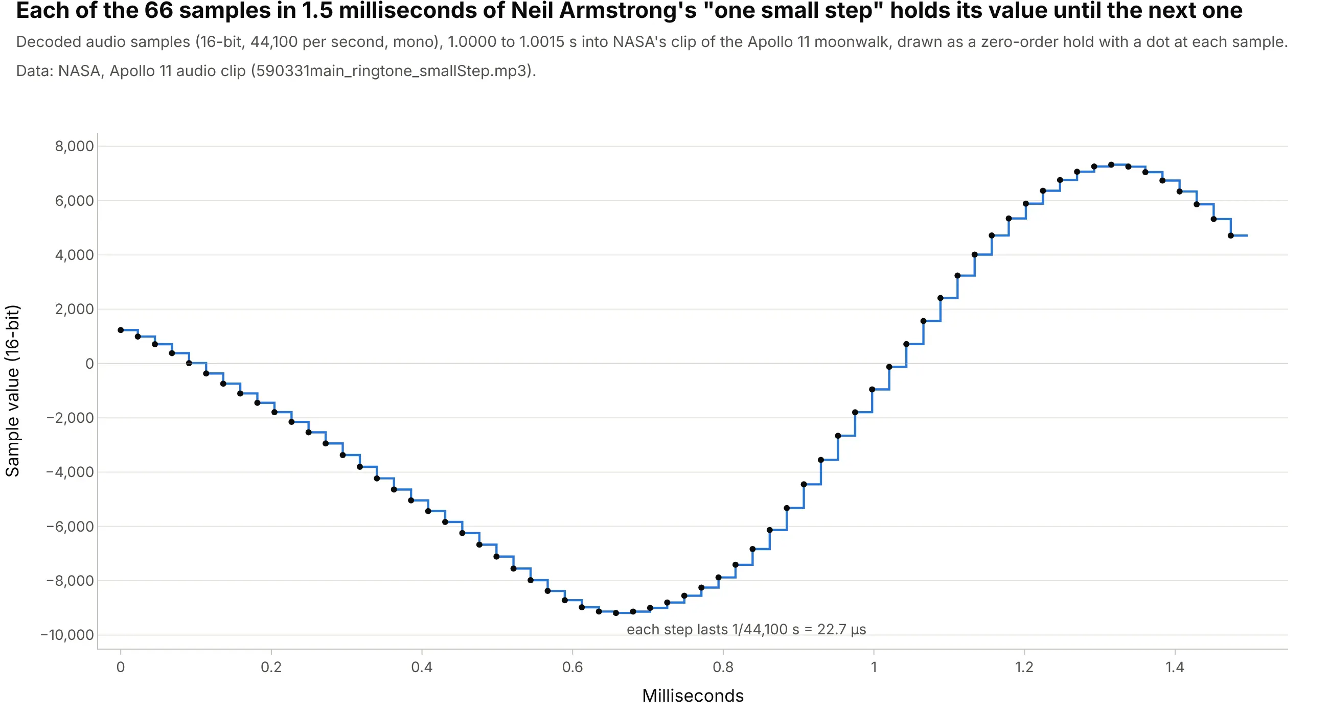
Sampled signals in engineering. Digital audio stores one number per sample, 44,100 a second, and a basic digital-to-analog converter holds each one for 22.7 microseconds until the next, which is the staircase MATLAB’s stairs function draws for discrete-time signals. Data: NASA, Apollo 11 audio clip.

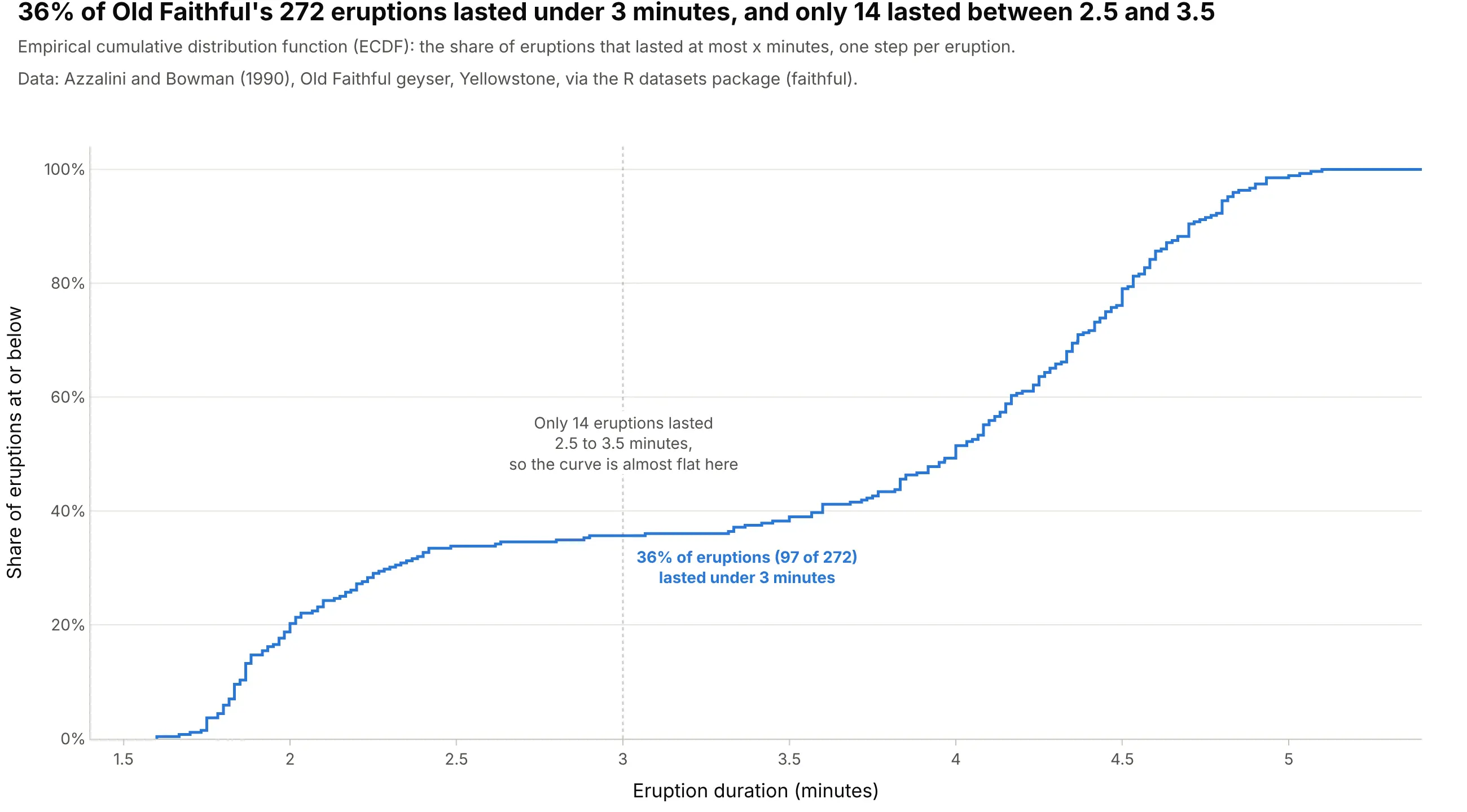
Distributions in statistics. An empirical cumulative distribution function (ECDF) is a step function that climbs at every observation, and on the classic Old Faithful geyser data it runs almost flat between 2.5 and 3.5 minutes because only 14 of 272 eruptions lasted that long. Data: Azzalini and Bowman (1990), via R’s faithful dataset.

Step chart or line chart?

A line chart joins its points with straight lines, and that tells the reader the value changed gradually between them. For a temperature or a stock price that’s a fair guess, because they move all the time and you only sampled them. For a value that someone sets, it’s wrong: the Fed’s rate didn’t drift from 0.50% to 1.00% between March 17 and May 5, 2022, it sat at 0.50% for 49 days and then jumped. Use a step chart when the value holds until it changes:

• Set by a decision: policy rates, prices and tariffs, tax rates, the minimum wage, a firmware version, or a setpoint on a controller
• Counts of things: the number of open orders, staff on shift, versions in support, planets discovered so far
• Levels with discrete changes: inventory between deliveries, a battery’s state between charges in a log, a stepper motor’s position
• Statistical step functions: ECDFs, Kaplan-Meier survival curves, and cumulative event counts, where every jump is one observation
• Sampled signals: a sensor read once a second or an audio signal, drawn as the zero-order hold a digital-to-analog converter outputs

Use a line chart for quantities that change continuously between measurements, like a temperature, a flow rate, or a share price, and use a bar chart when each value belongs to a whole period, like monthly sales, and you want to compare the periods with each other.

How line_shape works: hv, vh, hvh, and vhv

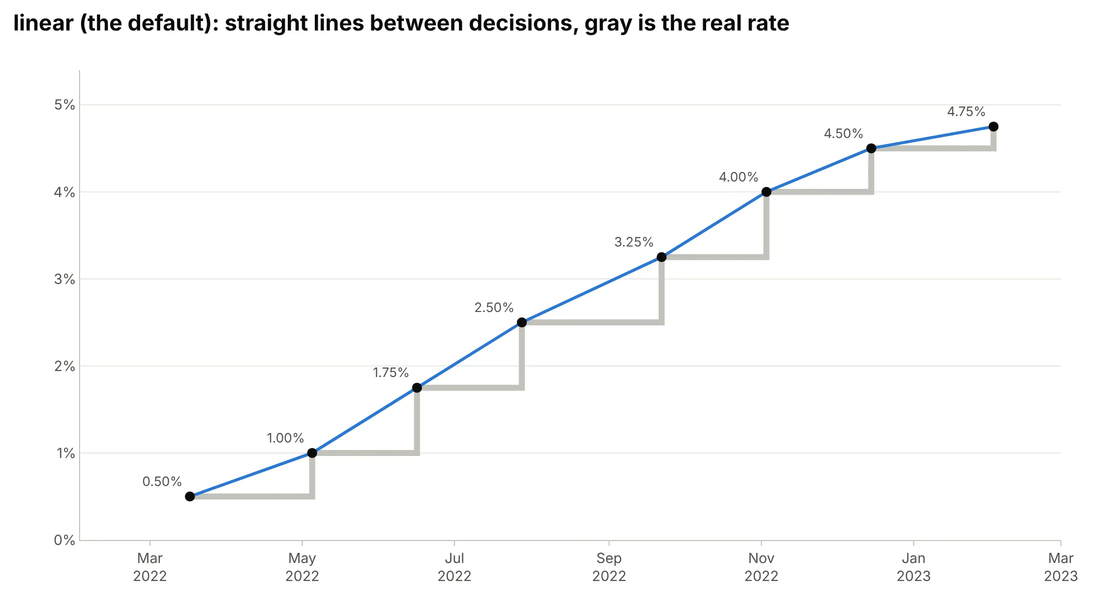
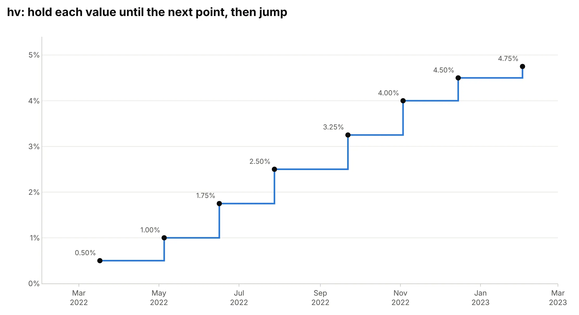
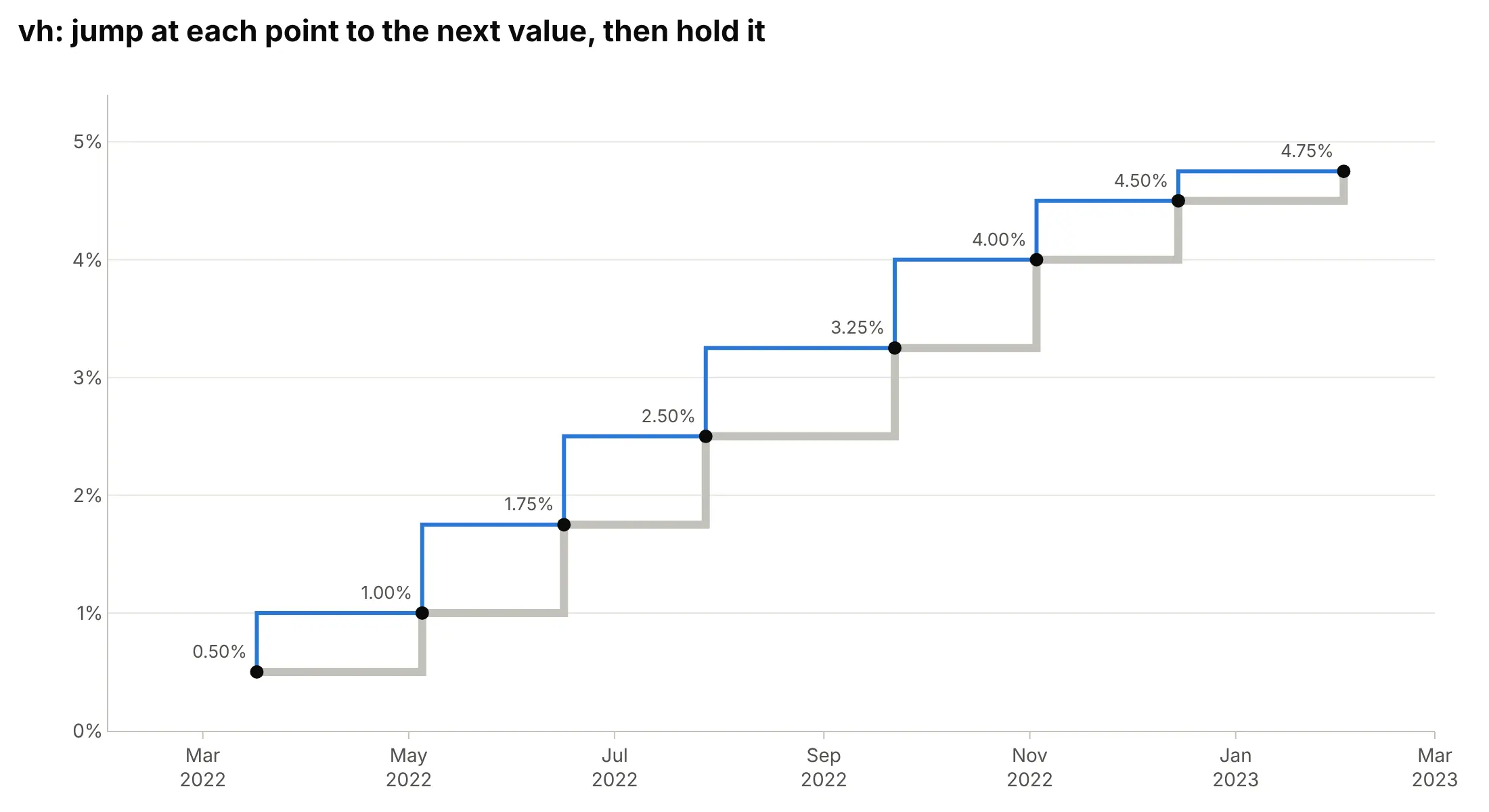
Plotly draws a step chart by changing how it connects the points. line_shape="linear" is the default; the four step shapes are named after the order in which they draw the horizontal (h) and vertical (v) parts of each connection. Here are the Fed’s eight changes from March 2022 to February 2023 drawn each way, with the true path in thick gray behind each one.

linear draws straight lines between points. Around April 10, 2022 it reads 0.75%, a rate that was never in force, and it makes the 2022 hikes look like one smooth climb:

hv goes horizontally first, then vertically: it holds each value until the next point’s date, then jumps. That’s right when each date is the start of the value, as here, where FRED dates every range by the day it took effect:

vh goes vertically first: it jumps at each point to the next point’s value, then holds that. That’s right when each date is the end of the value, such as a monthly average stamped on the last day of the month or a meter reading that covers the half hour before it. On start-dated data like this, every step lands one decision early, so 1.00% appears on March 17, seven weeks before the Fed set it:

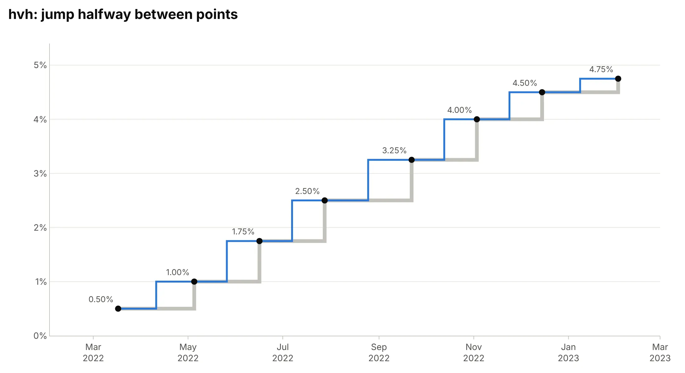
hvh jumps halfway between two points. That’s right when each value applies to the time around its point, such as a reading taken in the middle of its interval or data stamped at the center of each day. On these decisions every hike shows up about three weeks early:

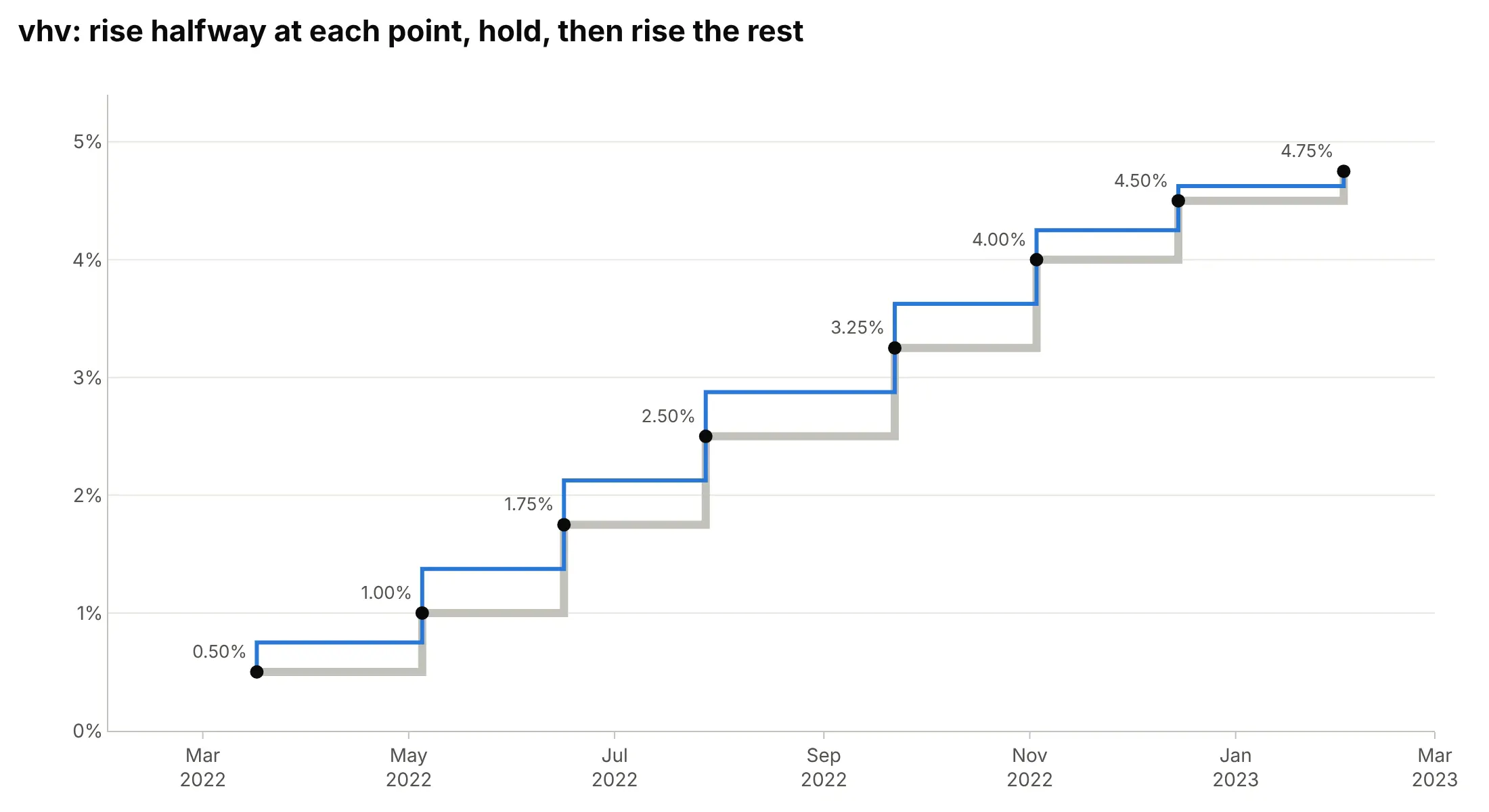
vhv goes halfway up at each point, across, then up the rest of the way, so its flat parts sit halfway between two values (0.75%, 1.375%, and so on), which a time series never wants. It’s the y-axis version of "hvh", for charts where y is the input and x the value, like a vertical profile of temperature against depth:

Two more details decide whether the steps land on the right dates:

• Check which date your data uses. A central bank announces a decision on one day and it takes effect on another, a tariff is published weeks before it starts, and a sensor log can stamp a reading when it starts or when it’s written. Pick "hv" for start dates and "vh" for end dates, and say in the subtitle which one the chart uses.
• Give the last value a width. With "hv", the last point is where the line stops, so the current value appears as a single point with nothing after it (look at 4.75% in the hv chart above). Add one more point with the same value at today’s date, or at the end of the period, as the main example does with November 6, 2026.

Matplotlib names the same choices differently: plt.step(where="post") is Plotly’s "hv", where="pre" (its default) is "vh", and where="mid" is "hvh". In pandas, df.plot(drawstyle="steps-post") is "hv".

A short history

Step charts have no single inventor, because they draw the step function, one of the oldest ideas in mathematics: a function that is constant over each of a few intervals. Its simplest form, the unit step that is zero before a point and one after it, is named after the electrical engineer Oliver Heaviside and is a tool of the operational calculus he used for circuits (Wikipedia). In signal processing the same staircase is the zero-order hold, the output of a digital-to-analog converter that holds each sample until the next, and in statistics the survival curve that Kaplan and Meier (1958) showed how to estimate from incomplete observations is a step function that drops at each event. We couldn’t find a first published step chart of prices or rates to redraw. Today every plotting library has one: MATLAB’s stairs draws a “stairstep graph” (MathWorks), Matplotlib has step and stairs, and in Excel, where step charts “are not native”, people build them by duplicating rows (Peltier Tech).

Alternatives to a step chart

Here’s the Fed’s target rate from 2015 to 2026 drawn six ways. Some are better for the question, some worse, some just different:

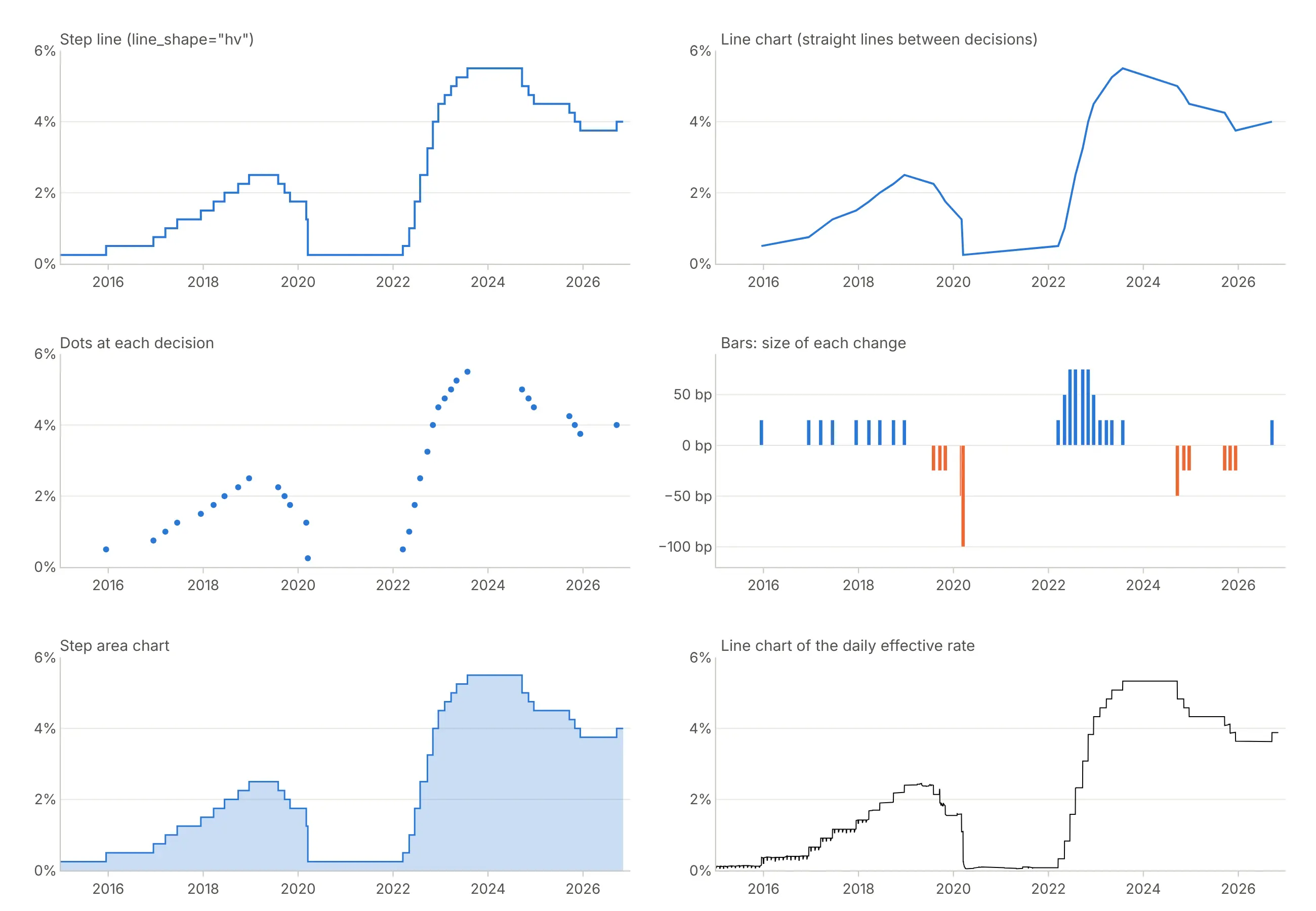
• Line chart through the decisions (worse). The diagonals invent rates between decisions, and the two years at 0.25% from March 2020 to March 2022 become a slow ramp up to 0.50%.
• Dots at each decision (worse for levels). Each dot is correct, but readers can’t tell what the rate was between dots, and long gaps such as 2020 to 2022 look empty.
• Bars of each change (different). Bars of the size of each move, in basis points (bp, hundredths of a percentage point), show the four 75 bp hikes of 2022 and the 100 bp cut of March 2020 better than any other view, but readers have to add them up to get the level.
• Step area chart (works too). Filling under the steps keeps every date correct and gives the chart more weight; use it for one series, since filled areas hide each other.
• Line chart of the daily effective rate (works too, for market data). The rate banks actually paid changes every day, so an ordinary line is right for it, and it lands inside the target range on 99.9% of days.

A Gantt chart is the better choice when you care about which items were active rather than how many, as the Python versions example below shows.

How to make a step chart

With AI

ChatGPT, Claude Code, GitHub Copilot, Cursor, and other AI tools are excellent at writing Plotly code. Name Plotly in the prompt, and say whether each date is the start or the end of a value and what the last step should run to:

With Plotly Studio

Plotly Studio is a desktop app where you point an AI at a dataset and it builds charts and a Dash app around your questions. Ask for a step chart the same way:

Show the electricity unit rate as a step chart with line_shape="hv" from valid_from, the current rate extended to today, a dropdown to pick the region, and the rate and its dates on hover.

Make a step chart in Python or JavaScript

This is the code AI tools write under the hood. In Plotly Express, a step chart is px.line with line_shape="hv":

Most step data arrives as a list of changes, such as a price with a valid_from date, with no row for today. This helper repeats the last value at a date you pass, so the last step has a width, and every example in this guide uses the same idea:

In JavaScript, plotly.js draws a step chart with line: {shape: "hv"} on a scatter trace:

Share it

Every Plotly chart has a Share chart button (the cloud icon in its toolbar) that uploads it to Plotly Cloud and gives you a link. Only you can see it until you change its visibility.

For a live app, put the chart in a Dash app and publish it with the Plotly Cloud CLI. Coding agents can run these commands for you:

If your data has to stay in your own cloud or data center, publish to Dash Enterprise instead.

Dos and don’ts

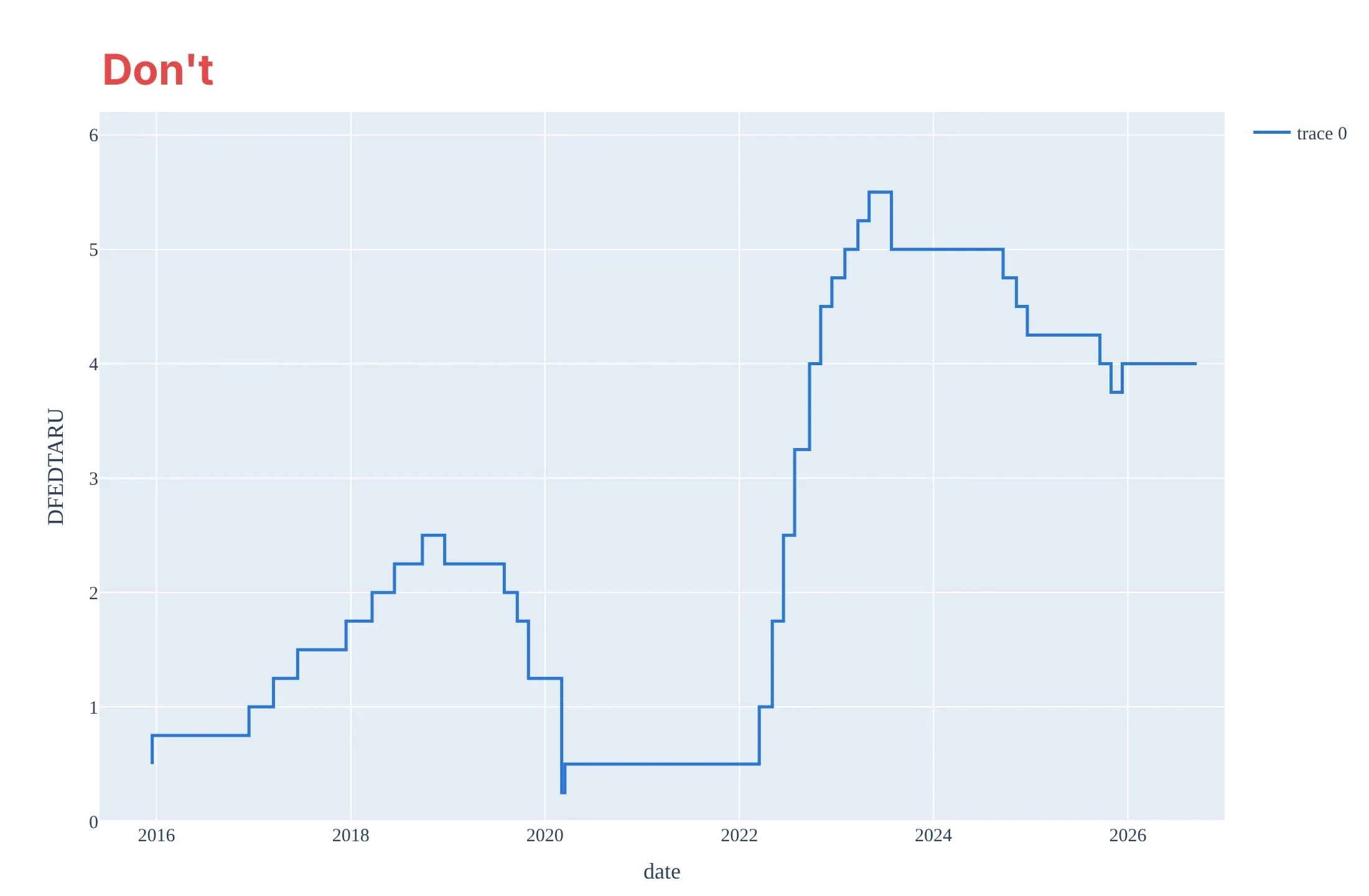
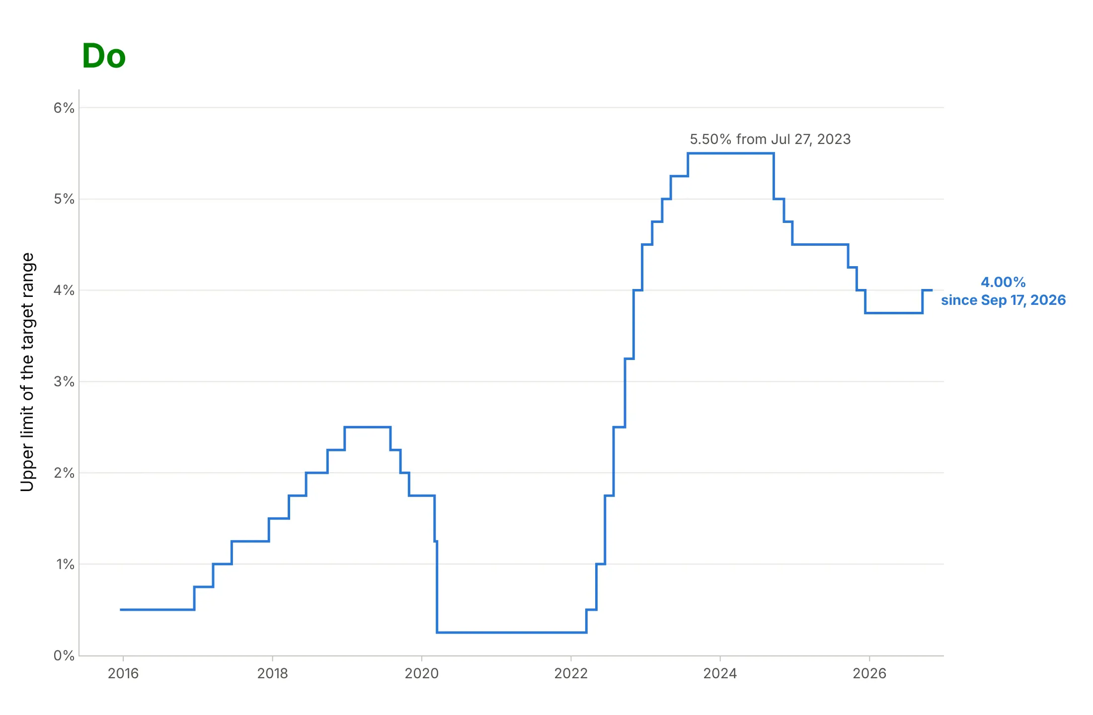
Most mistakes in a step chart put the steps on the wrong dates, and the chart still looks fine. Here is the upper limit of the Fed’s target range from December 2015 to November 2026 both ways, in the same blue.

Don’t use line_shape="vh" on data dated by the day each value took effect (here it shows 0.50% from March 2020 to March 2022, when the rate was 0.25%, and 4.00% from December 2025, nine months before the Fed set it), stop the data at the last change so the current level has no step, or keep the raw column names, a one-trace legend, and a serif font:

Do use "hv" for start-dated data, extend the last value to the latest date, add a percent sign to the ticks, and label the current level and the peak with their dates:

Checklist

Do

• Find out whether each date is the start, the end, or the middle of its value, and pick "hv", "vh", or "hvh" to match.
• Repeat the last value at today’s date (or the end of its period) so it gets a step.
• Keep only the rows where the value changed when you have daily data, which makes the hover text and the file smaller.
• Label the current level and the changes that matter, with their dates.
• Use a step area (fill="tozeroy") for a single series when the total matters, such as a count.
• Draw continuous data next to it as an ordinary line, as the effective rate and the inflation-adjusted minimum wage are drawn here.

Don’t

• Use a straight line or a spline for values that hold until they change.
• Add markers at every point of a long daily series; mark the changes instead.
• Stack many overlapping step lines with the same values, since they hide each other; offset them slightly, use small multiples or label each line.
• Use "vhv" on a time series; it draws levels halfway between two values.

Options to customize

A step chart in Plotly is a scatter trace with a step line_shape, so these are the options that matter most. The full lists are in the scatter trace reference and the line charts documentation.

1. line_shape="hv" (line.shape in JavaScript): the step line; "vh" for end-dated data, "hvh" for steps halfway between points, "vhv" for charts with y as the input
2. px.line(..., line_shape="hv"): the same in Plotly Express, with one step line per color group
3. fill="tozeroy" or fill="tonexty": a step area chart, or a band between two step lines such as a target range
4. mode="lines+markers": dots on the points themselves, for short series or sampled signals
5. connectgaps=False (the default): leave None in the data to break the steps where values are missing
6. hovertemplate: the value and the date it took effect, such as "from %{x|%b %d, %Y}<br>%{y:.2f}%"
7. fig.add_annotation: the current value at the right end, and labels on the steps that matter
8. go.Scattergl: WebGL for hundreds of thousands of steps; it supports "hv", "vh", "hvh", and "vhv" too (but not "spline")
9. xaxis.type="category": equal-width steps for ordered categories such as software versions; keep a date or numeric axis when the time between changes matters

More step chart examples

Six more step charts built from real public data, each with its source, the technique that makes it work, and a prompt to rebuild it.

1. Half-hourly electricity prices that went negative for 16 hours

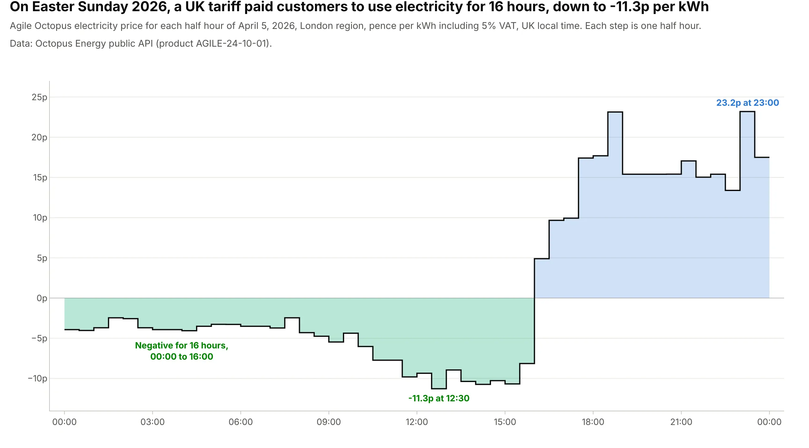
On Easter Sunday 2026, the Agile Octopus tariff in London paid customers to use electricity for 16 hours straight, with a low of -11.3p per kWh at 12:30. Each price holds for exactly half an hour, so the steps show the price at every minute. Data: Octopus Energy public API (Agile Octopus, London region, including 5% VAT).

Tip: draw two step areas, one clipped below zero and one above, to color negative prices differently, and repeat the last price at midnight so 23:30 gets its full half hour.

2. The US federal minimum wage, in dollars of the day and in 2026 dollars

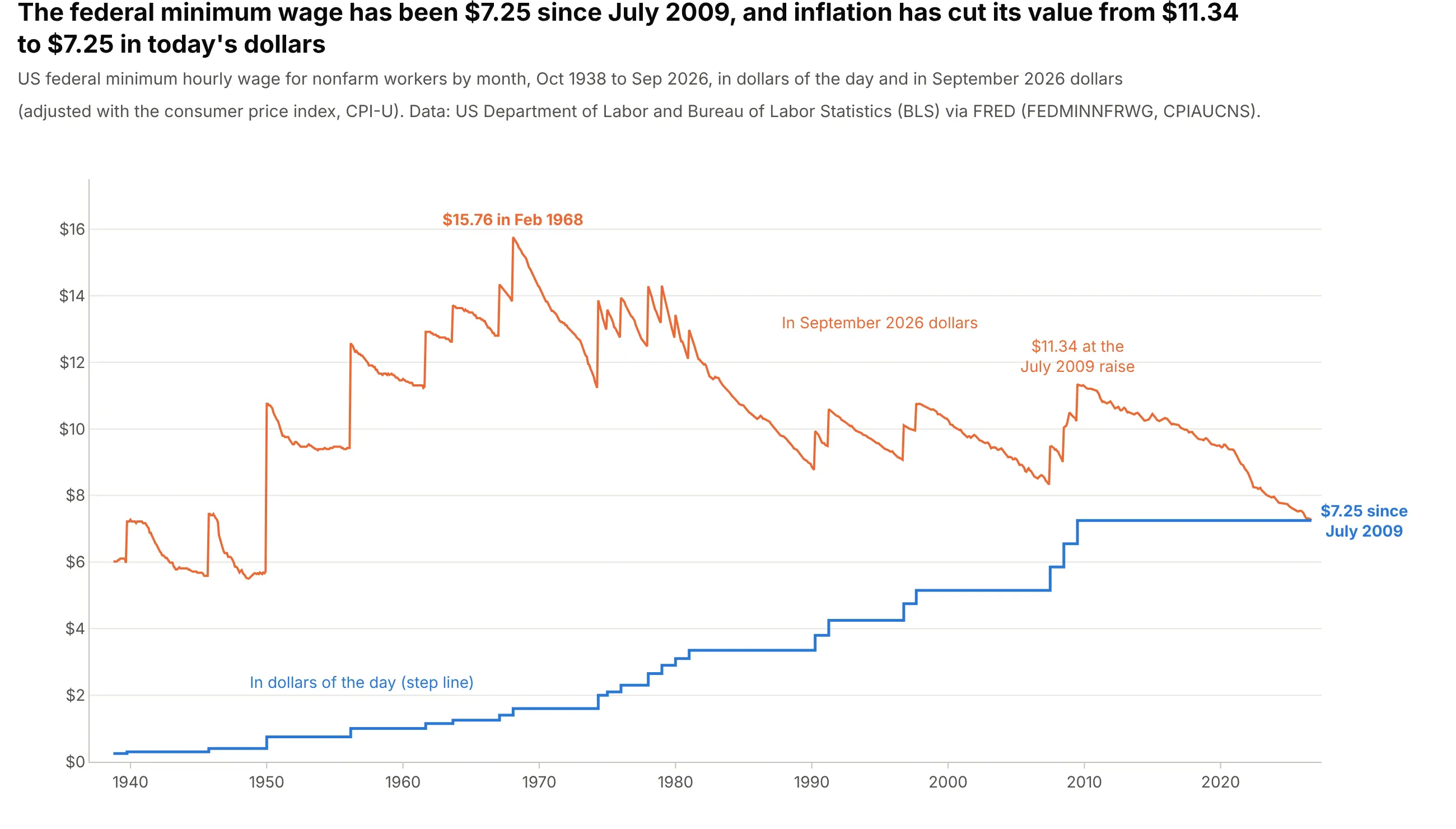
The federal minimum wage has been $7.25 an hour since July 2009, the longest stretch without a raise since it began in 1938, and inflation has cut its value from $11.34 to $7.25 in September 2026 dollars. The legal minimum is a step function and its real value is not, so the chart draws one as steps and the other as a line. Data: US Department of Labor and Bureau of Labor Statistics (BLS) via FRED (FEDMINNFRWG, CPIAUCNS).

Tip: draw a value set by law as steps and anything derived from a continuously changing index, like an inflation adjustment, as an ordinary line.

3. Three central banks’ policy rates since 2019

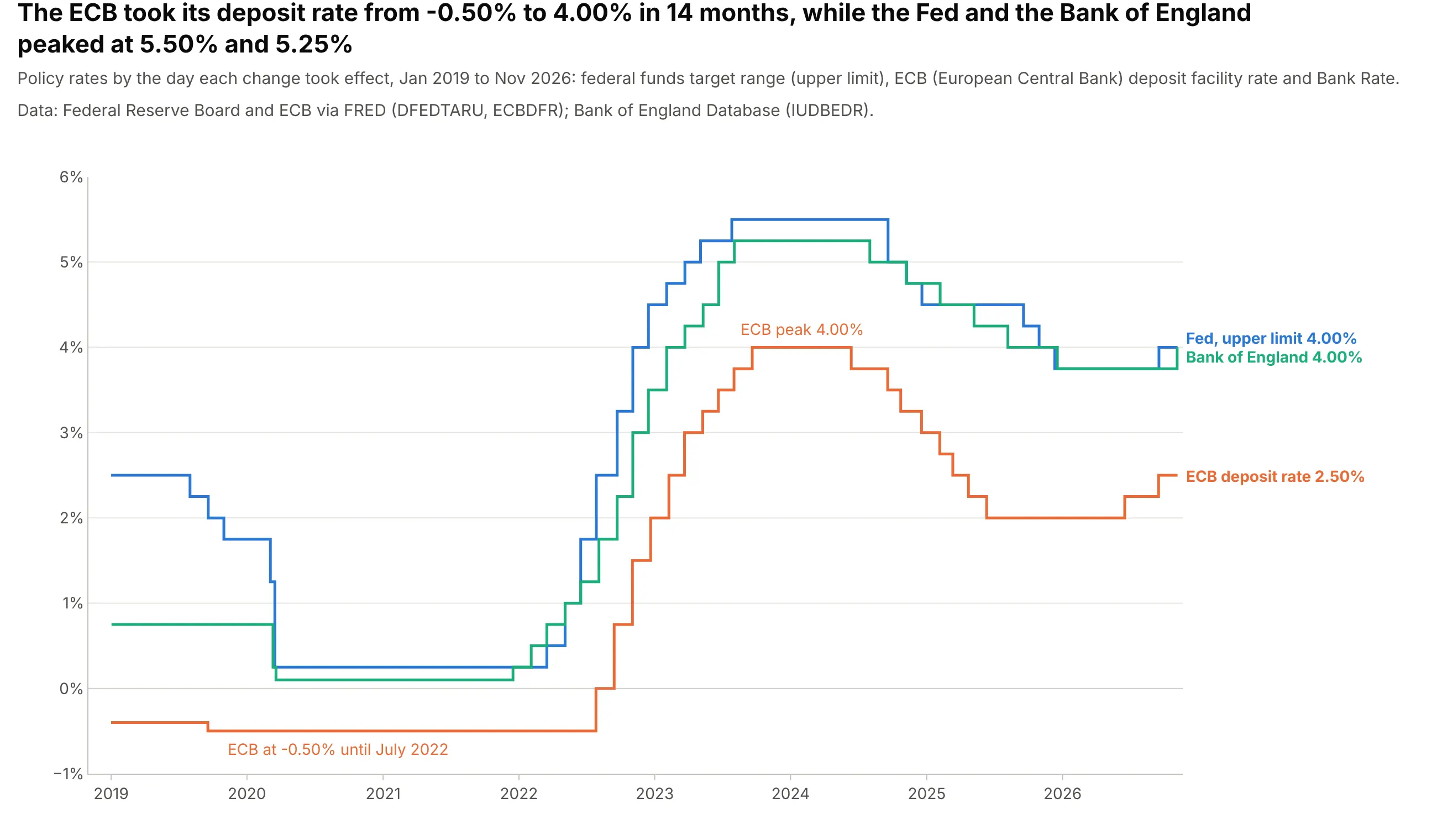
The European Central Bank (ECB) took its deposit rate from -0.50% to 4.00% in 14 months, from July 2022 to September 2023, while the Fed and the Bank of England peaked at 5.50% and 5.25%. Each bank decides on its own dates, and step lines let you compare them on any day without lining the dates up first. Data: Federal Reserve Board and ECB via FRED (DFEDTARU, ECBDFR); Bank of England Database (IUDBEDR).

Tip: label each line at its right end with its current value instead of using a legend.

4. Marginal and average tax rates on income

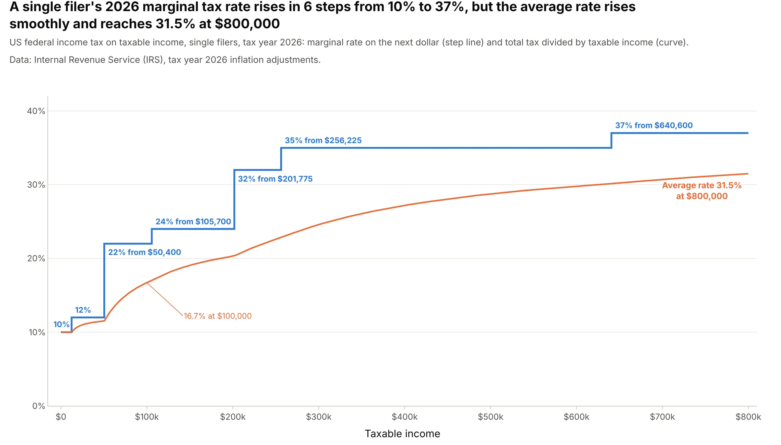
A single filer’s 2026 marginal tax rate rises in six steps from 10% to 37%, while the average rate, total tax divided by income, rises smoothly and is 16.7% at $100,000 and 31.5% at $800,000. The x axis here is income, not time: step charts work for any value that’s constant over ranges. Data: Internal Revenue Service (IRS), tax year 2026 inflation adjustments.

Tip: label each step with its rate and threshold right on the line, and draw the average rate on top to show that crossing a threshold only raises the rate on the dollars above it.

5. How many Python versions were supported at once

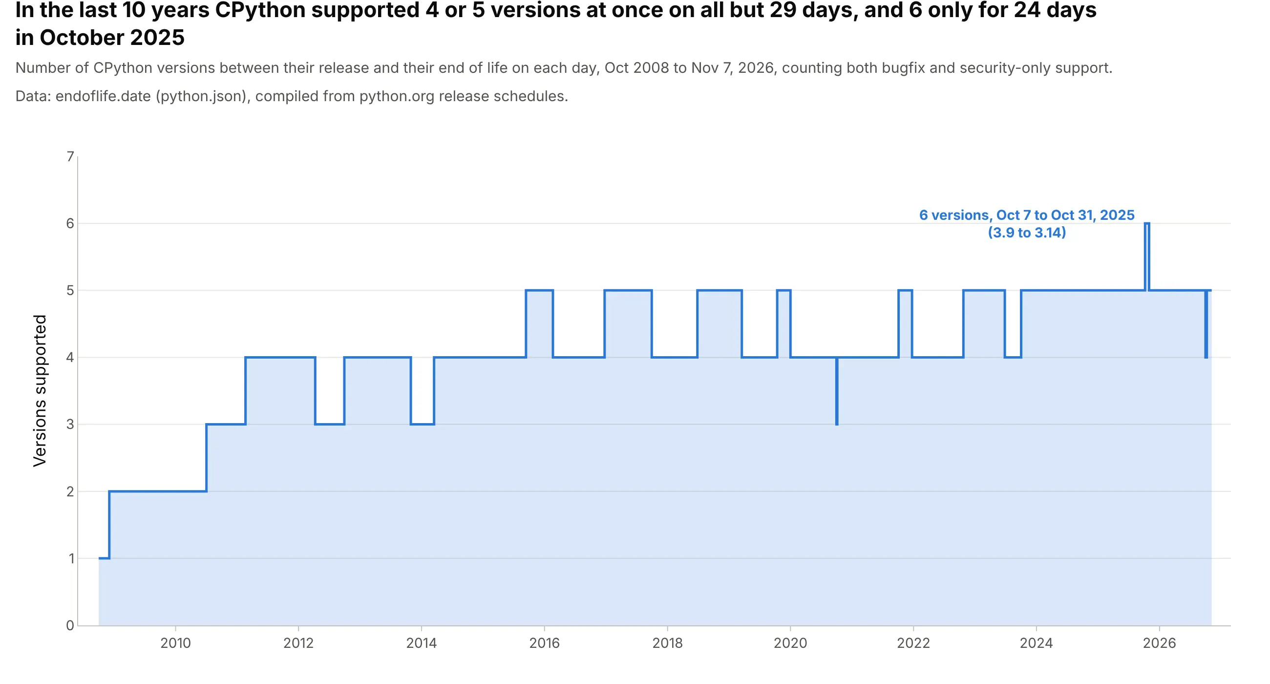
From November 2016 to November 2026, CPython had four or five versions in support on all but 29 days, and six only for 24 days in October 2025, between the release of 3.14 and the end of life of 3.9. A count changes only when something starts or ends, so a step area is exact. Data: endoflife.date, compiled from python.org release schedules.

Tip: compute the count only at the dates where something starts or ends, then let line_shape="hv" fill in the days between.

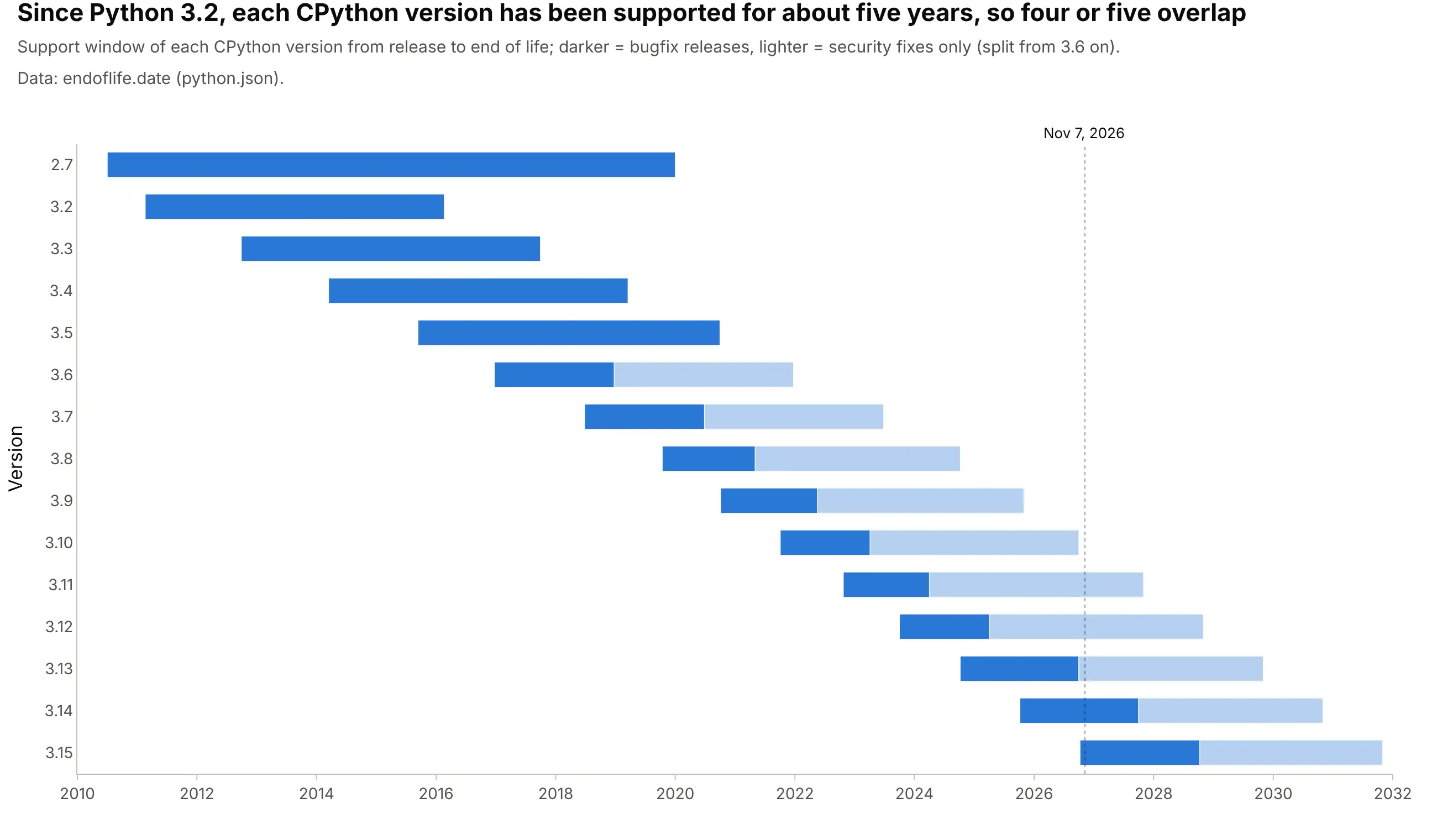
Another way to see it: a Gantt-style timeline shows which versions overlap, with bugfix and security-only support in two shades, and you count the bars to get the step chart’s value:

6. Confirmed exoplanets, and the months that added hundreds

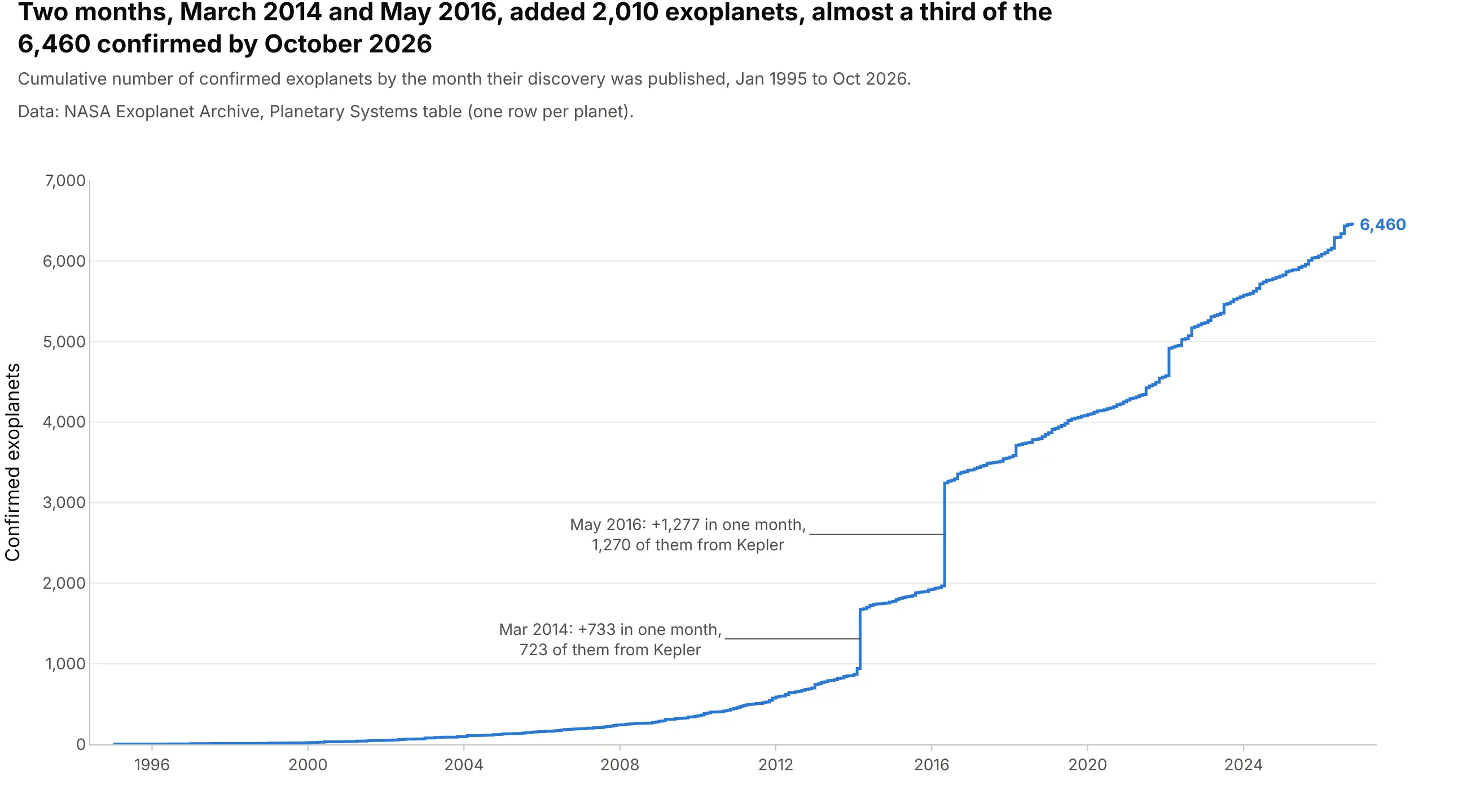
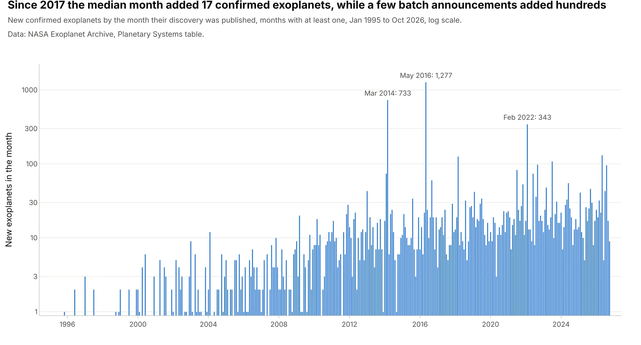
Two months, March 2014 and May 2016, added 2,010 of the 6,460 exoplanets confirmed by October 2026, almost a third, and 1,993 of those 2,010 came from NASA’s Kepler space telescope, whose results were published in large batches. In a cumulative count, a step line makes each batch a vertical jump instead of a slope spread across the month before. Data: NASA Exoplanet Archive, Planetary Systems table.

Tip: annotate the biggest jumps with the size of the batch, since a cumulative chart makes readers estimate it from the axis.

Another way to see it: bars of the new planets per month, on a log axis, show that the median month since 2017 added 17 planets, and that the batches stand out by a factor of 20 to 75: