Psychrometric Charts - A Complete Guide

TL;DR

• A psychrometric chart is the map of moist air that heating, ventilation and air-conditioning (HVAC) engineers design with: dry-bulb temperature on the x axis, humidity ratio (grams of water per kilogram of dry air) on a y axis on the right, and curved lines of relative humidity (RH) that end at the saturation curve, where air can hold no more water.
• Diagonal lines on the same chart give the wet-bulb temperature and the enthalpy (heat content), and steep lines give the specific volume, so one point tells you seven properties of the air. In much of Europe the same physics is drawn as the Mollier h-x diagram, and the chart is similar to a scatter plot with a grid of physics drawn behind it, like the Smith chart or a carpet plot.
• Engineers draw air-conditioning processes on it as arrows (heating is horizontal, evaporative cooling follows a wet-bulb line, a cooling coil moves down and to the left), shade the comfort zone of ASHRAE Standard 55 (the American Society of Heating, Refrigerating and Air-Conditioning Engineers' thermal comfort standard), and plot a year of weather on it to choose a cooling strategy.
• You can make a psychrometric chart with Plotly from go.Scatter lines computed with the psychrolib package, which implements the ASHRAE Handbook formulas, with your data on top as a marker trace. The code is below.

What is a psychrometric chart?

Psychrometric charts look like this:

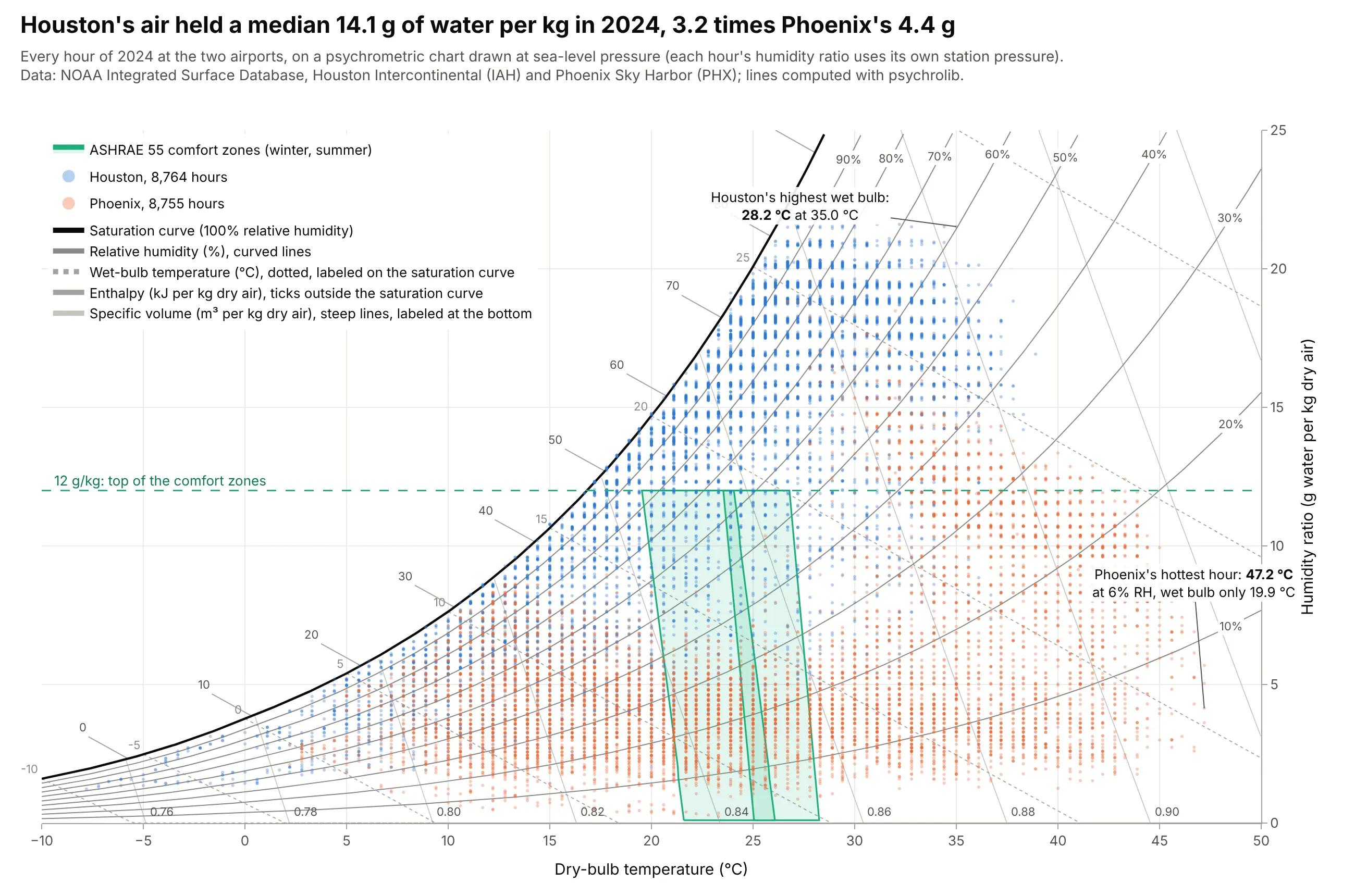
Data: hourly airport observations from NOAA's (the National Oceanic and Atmospheric Administration's) Integrated Surface Database, Houston Intercontinental and Phoenix Sky Harbor, 2024; lines computed with psychrolib.

How do you read a psychrometric chart? In the example above, notice these things:

• Each dot is one hour of 2024. Its position across is the air temperature, and its height is how much water the air held, in grams per kilogram of dry air. Houston's air held a median 14.1 g/kg and Phoenix's 4.4 g/kg, 3.2 times less, which is why Houston's cloud sits high and Phoenix's sits low. The dots fall in stripes because NOAA reports temperature and dew point to a tenth of a degree or a whole degree, so many hours share the same values; the data is plotted as reported, without jitter.
• The black saturation curve is the most water air can hold at each temperature, and it roughly doubles with every 10 to 12 degrees C. The gray curves under it are relative humidity, the share of that maximum. Phoenix's hottest hour, 47.2 degrees C, was at only 6% relative humidity.
• The dotted diagonals are wet-bulb temperatures, the coolest that evaporating water can make the air. Phoenix's hottest hour had a wet bulb of 19.9 degrees C, while Houston's highest wet bulb of the year was 28.2 degrees C at 35.0 degrees C, so in Houston sweat and evaporative coolers stop working well long before Phoenix's heat does.
• The green areas are the ASHRAE Standard 55 comfort zones for winter and summer clothing, capped at 12 g/kg. Houston's air was above that cap in 59.9% of hours of 2024 and Phoenix's in 5.4%, so Houston's buildings spend most of the year removing water as well as heat.

It's often used for charts like these:

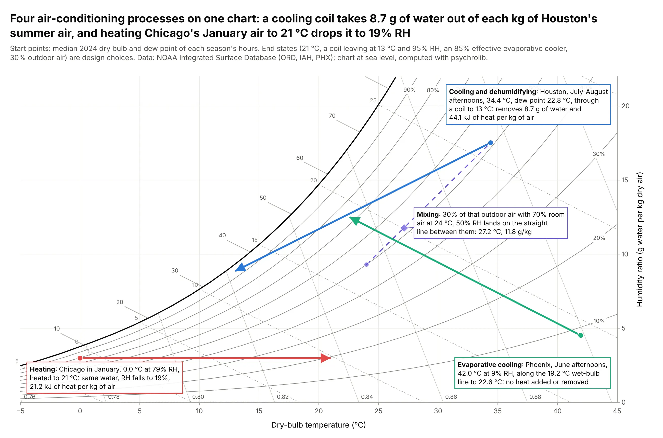
Air-conditioning processes. The textbook use: every process is a straight move, and the length of each arrow on the two axes is the heat and water to add or remove. Cooling Houston's median summer afternoon (34.4 degrees C, dew point 22.8 degrees C) through a coil to 13 degrees C takes out 8.7 g of water and 44.1 kJ of heat per kg of air. Data: NOAA Integrated Surface Database, 2024 (Chicago, Houston, Phoenix); the end states are design choices, not measurements.

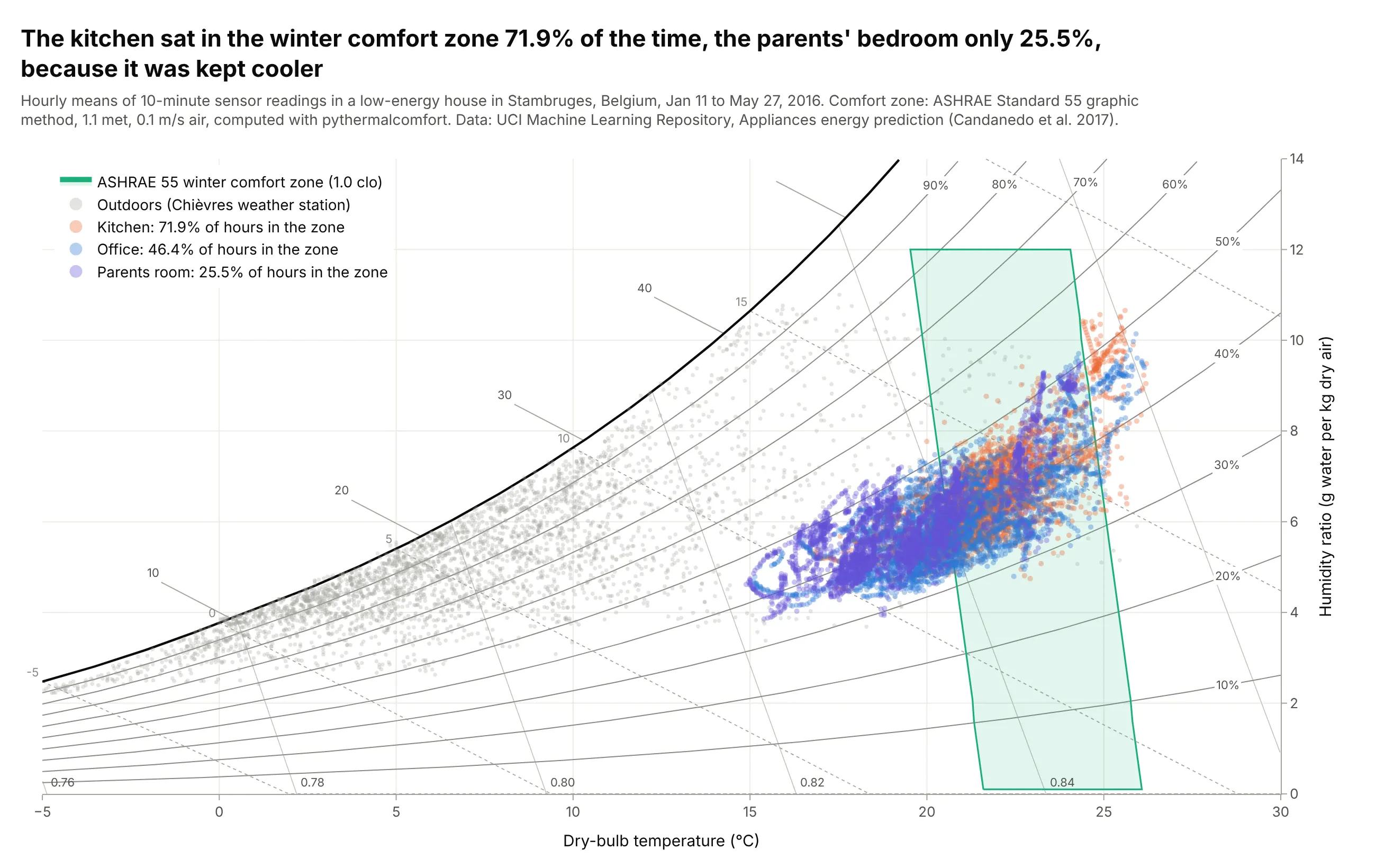
Comfort zones and building monitoring. Indoor sensors plotted against the ASHRAE Standard 55 comfort zone show which rooms are too cool, too warm or too humid. In a low-energy house in Belgium, the kitchen was in the winter zone 71.9% of hours from January to May 2016, the parents' bedroom only 25.5%, because it was kept cooler. Data: UCI Machine Learning Repository, Appliances energy prediction (Candanedo, Feldheim and Deramaix 2017), CC BY 4.0.

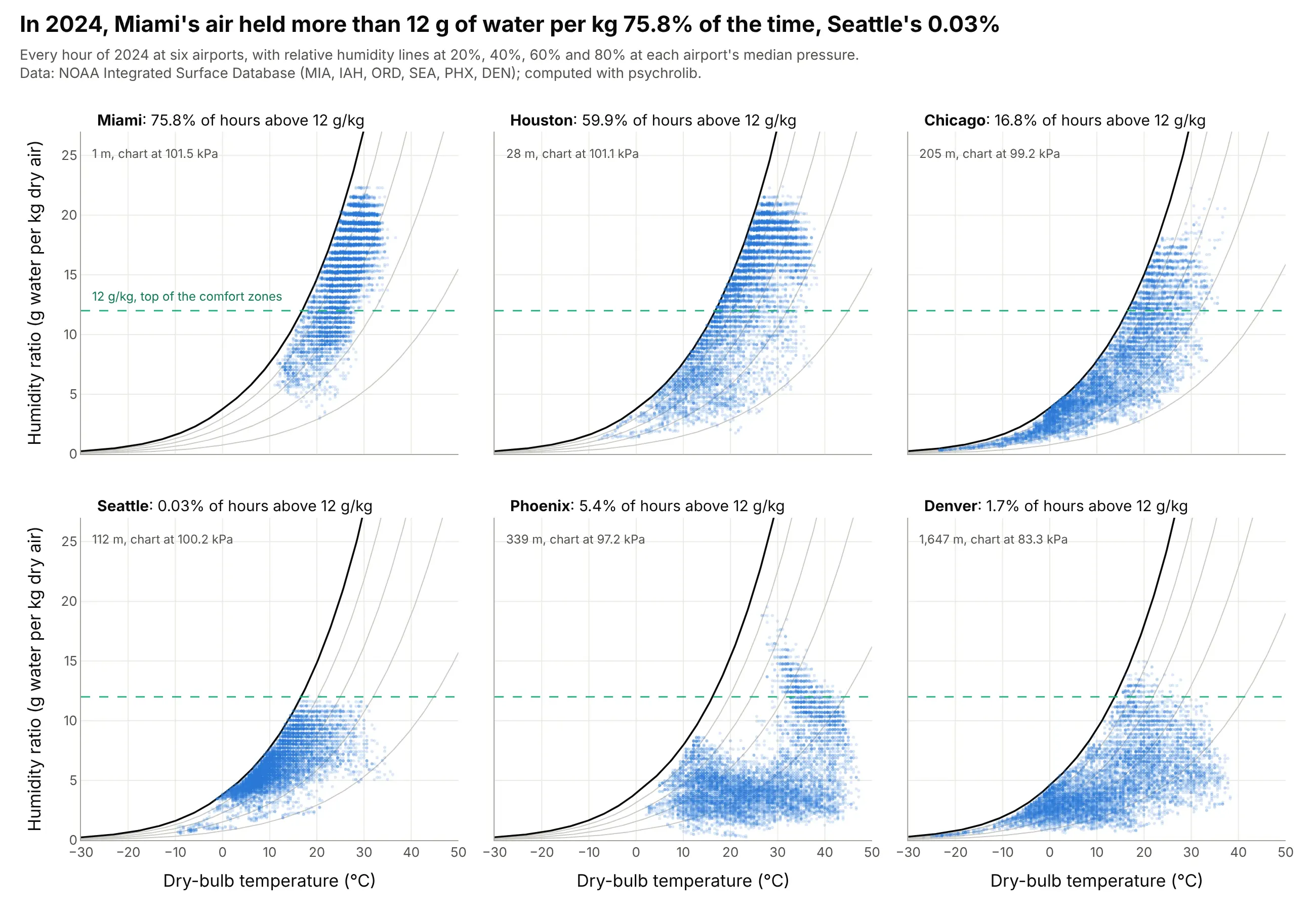
Climate analysis for building design. Architects and mechanical engineers plot a site's weather on the chart before they choose a cooling strategy. Miami's air held more than 12 g of water per kg in 75.8% of the hours of 2024 and Seattle's in 0.03%, so Miami needs dehumidification and Seattle mostly needs heat. Data: NOAA Integrated Surface Database, 2024, six airports, each chart drawn at its airport's median pressure.

How to read a psychrometric chart

A psychrometric chart puts seven properties of moist air on one page. Any two of them (plus the air pressure) fix the rest, so if you know where a point is, you can read off all the others. This is one point, Houston's median summer afternoon in 2024, read seven ways:

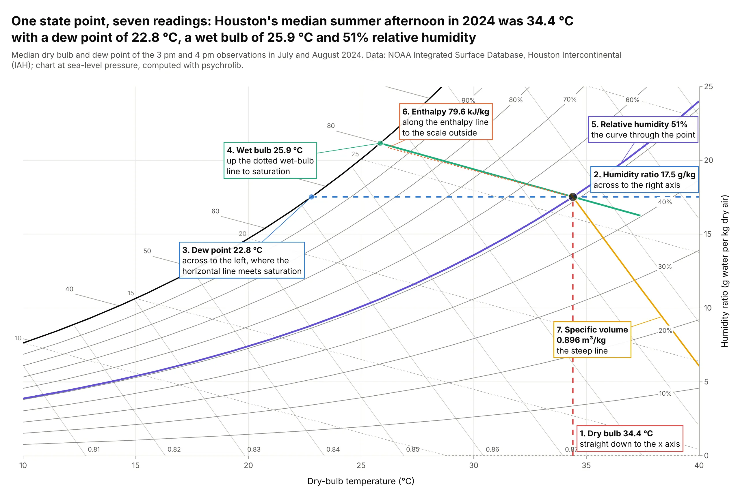
Data: median dry bulb and dew point of the 3 pm and 4 pm observations at Houston Intercontinental in July and August 2024, NOAA Integrated Surface Database; computed with psychrolib at sea level.

Dry-bulb temperature and humidity ratio (the two axes)

The dry-bulb temperature is what an ordinary thermometer reads, shielded from sunshine and moisture, and it runs along the x axis. The humidity ratio (also called the moisture content or mixing ratio) is the mass of water vapor carried by each kilogram of dry air, in grams per kilogram (g/kg) on SI charts and in grains per pound on US charts (7,000 grains make a pound). It runs up a y axis on the right, because the left side of the chart is taken by the curved edge where the air is saturated. Heating or cooling air without adding or removing water moves a point straight across, and adding or removing water moves it straight up or down.

Relative humidity and the saturation curve

Warm air can hold more water vapor than cold air: at sea level, saturated air at 20 degrees C holds 14.7 g/kg and at 30 degrees C 27.2 g/kg. The top-left edge of the chart, the saturation curve, joins those maximums, and it's also the 100% relative humidity line. Relative humidity is the share of that maximum the air holds (strictly, the ratio of the water vapor's pressure to its pressure at saturation), so the 50% line sits about halfway between the saturation curve and the x axis. Because the maximum rises with temperature, the same air has a lower relative humidity when it's warmer: the more-examples section has a Houston day where relative humidity runs from 84% to 28% while the water content barely changes.

Dew point

The dew point is the temperature at which the air's water would start to condense if you cooled it without changing its water content. On the chart, move left along the horizontal line from the point until you hit the saturation curve and read the temperature there. Houston's afternoon point has a dew point of 22.8 degrees C, so any surface colder than that (a cold drink, a cooling coil, a window) gets wet. Because the dew point depends only on the humidity ratio (and the pressure), meteorologists often quote it instead of the humidity ratio, and it is the temperature to compare with the surfaces in a building.

Wet-bulb temperature

The wet-bulb temperature is what a thermometer reads when its bulb is wrapped in a wet wick and air blows over it. Water evaporates from the wick and cools it until the air next to it is saturated, so the wet bulb is the coolest temperature evaporation alone can reach, and it's the limit for evaporative coolers, cooling towers and sweating. On the chart, follow the dotted diagonal from the point up and left to the saturation curve: Houston's afternoon point has a wet bulb of 25.9 degrees C. The further the point is from saturation, the bigger the gap between dry bulb and wet bulb, and the more cooling evaporation can do.

Enthalpy

Enthalpy is the heat content of the air, in kilojoules per kilogram of dry air (kJ/kg) counted from 0 degrees C dry air, including the latent heat stored in its water vapor. Lines of constant enthalpy are almost parallel to the wet-bulb lines, so ASHRAE charts draw them as a scale of ticks outside the saturation curve; follow the diagonal from a point out to that scale. Houston's afternoon point holds 79.6 kJ/kg. The difference in enthalpy between two points, multiplied by the mass of air moved, is the heating or cooling load, which is how engineers size equipment from the chart.

Specific volume

The specific volume is the space one kilogram of dry air (with its water) takes up, in cubic meters per kilogram, and it appears as steep lines labeled along the bottom. Houston's afternoon air takes 0.896 m³/kg. Fans move a volume of air, while loads are worked out per kilogram, so this is the conversion between them.

The chart is drawn for one pressure

Every line on a psychrometric chart depends on the air pressure. Standard charts are drawn at sea level (101.325 kPa), which Wikipedia says is common practice up to about 600 m of altitude. Higher up, the same vapor pressure is a bigger share of thinner air, so the humidity ratio at saturation goes up: the Denver example below draws the chart at 83.3 kPa, where saturated air at 20 degrees C holds 18.0 g/kg instead of 14.7.

The ASHRAE 55 comfort zone

ASHRAE Standard 55 defines thermal comfort with the predicted mean vote (PMV), Ole Fanger's model of how a large group of people would rate a room on a scale from -3 (cold) to +3 (hot). Its graphic comfort zone method shades, on a psychrometric chart, the temperatures and humidities where PMV stays between -0.5 and +0.5 for people at office work (1.0 to 1.3 met, a unit of metabolic rate) in still air, in winter clothing (1.0 clo, a unit of clothing insulation) or summer clothing (0.5 clo). The zones lean to the left at the top because humid air feels warmer, and they stop at a humidity ratio of 0.012 kg/kg (12 g/kg); above that, the standard asks for the full PMV calculation (Wikipedia, ASHRAE 55). The zones in this guide are computed with pythermalcomfort, which implements the standard's PMV code, at 1.1 met and 0.1 m/s air speed.

A short history

Willis Carrier, the engineer who built one of the first modern air-conditioning systems, presented "Rational Psychrometric Formulae" to the American Society of Mechanical Engineers in December 1911 (full text on Wikisource; Wikipedia calls it the "Magna Carta of Psychrometrics"). Its charts already had today's layout: dry bulb along the bottom, the weight of water per pound of dry air up the side, the saturation curve, and "diagonal adiabatic lines ... representing saturation or wet-bulb temperatures". Wikipedia, citing Gatley (2004) in the ASHRAE Journal, dates Carrier's first chart to 1904. This is the range of his Fig. 1, redrawn with today's formulas, with the worked example from the paper:

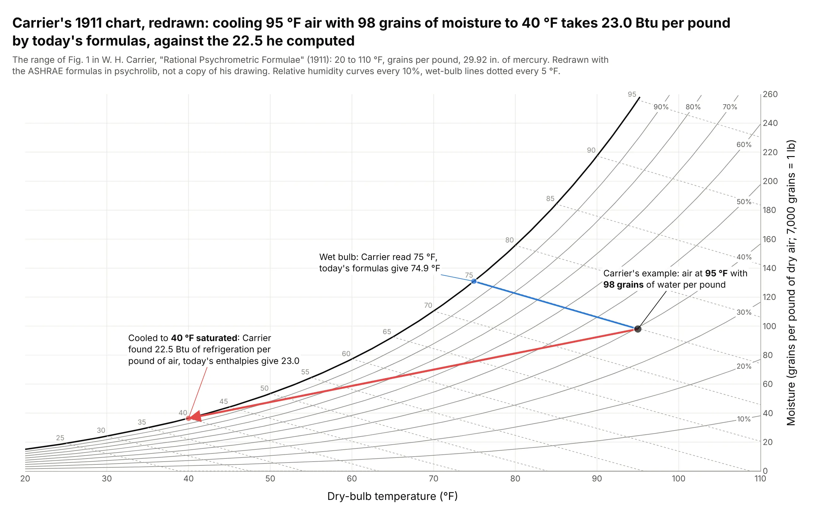
Data: computed with psychrolib in inch-pound (IP) units at 29.92 inches of mercury, Carrier's standard pressure; the example is from paragraph 87 of W. H. Carrier, "Rational Psychrometric Formulae", Journal of the American Society of Mechanical Engineers 33(11), 1911.

Carrier asked for "the refrigeration necessary to cool 1 lb. of air containing 98 grains of moisture and having a dry bulb temperature of 95 deg., to a final temperature of 40 deg. saturated", read a wet bulb of 75 degrees F from his chart, and answered 22.5 Btu (British thermal units) per pound. Today's ASHRAE formulas give 23.0. In 1923 Richard Mollier published the h-x diagram, with enthalpy and humidity ratio as its coordinates, which engineers in Germany, Scandinavia, Eastern Europe and much of the rest of Europe still use (Wikipedia), and ASHRAE's own charts have used similar oblique enthalpy coordinates since 1961.

Alternatives to a psychrometric chart

Here's the same Houston and Phoenix weather drawn six ways. Some are better for the question, some worse, some just different:

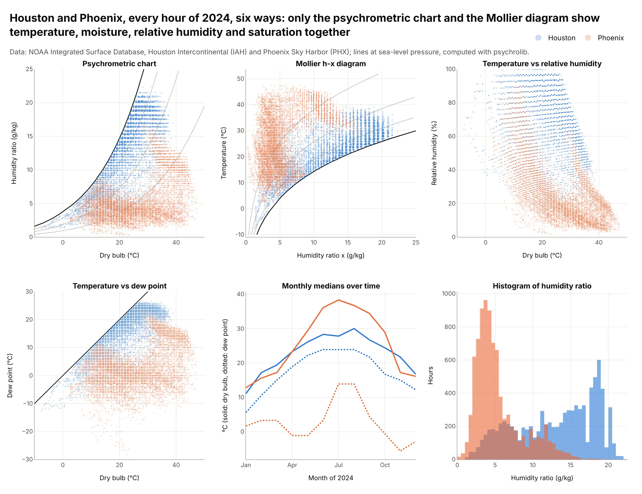
• Mollier h-x diagram (works too). The same physics turned on its side, with temperature up the side and humidity ratio across. Use it when your readers were trained in Europe; the example under More examples shows it in full.
• Temperature against dew point (works too, for weather). The dew point carries the same information as the humidity ratio at a given pressure, and the diagonal where the two are equal is the saturation line. Meteorologists read this more easily, but there are no enthalpy or wet-bulb lines to design with.
• Temperature against relative humidity (worse). Relative humidity falls when the temperature rises even if the water content doesn't change, so every daily cycle smears into a diagonal band and the two climates overlap.
• Monthly medians over time (different). A line chart shows when the humid months come, which the psychrometric chart hides, but not how temperature and moisture combine in each hour.
• Histogram of humidity ratio (different). A histogram compares how much water each city's air holds, but drops temperature entirely.

For a year of hourly points, a 2D histogram or density contour on psychrometric axes shows where the hours pile up better than overlapping dots, and small multiples of psychrometric charts, as in the six-city example above, compare sites without overplotting.

How to make a psychrometric chart

With AI

ChatGPT, Claude Code, GitHub Copilot, Cursor and other AI tools are excellent at writing Plotly code. Name Plotly in the prompt, and ask for the lines to be computed with psychrolib so the physics is right:

With Plotly Studio

Plotly Studio is a desktop app where you point an AI at a dataset and it builds charts and a Dash app around your questions. Ask for a psychrometric chart the same way:

Show every hour of this weather file on a psychrometric chart: dry bulb on x, humidity ratio in g/kg on the right axis, relative humidity and wet-bulb lines computed with psychrolib at the site's pressure, the ASHRAE 55 comfort zone shaded, and a dropdown to pick the month.

Make a psychrometric chart in Python or JavaScript

This is the code AI tools write under the hood. You can make a psychrometric chart with Plotly from go.Scatter lines computed from the physics of moist air, with a right-hand y axis and your data on top. This helper returns a go.Figure, and every example in this guide builds on the same idea:

psychrolib (pip install psychrolib) implements the moist-air formulas of the ASHRAE Handbook Fundamentals in SI and IP units (Meyer and Thevenard 2019); call psy.SetUnitSystem(psy.IP) for a chart in degrees F and pounds. This snippet is the core of every chart in this guide. The full version adds enthalpy ticks outside the saturation curve, specific volume lines, line labels, the ASHRAE 55 comfort zone polygons and the hover text with relative humidity, dew point and wet bulb.

In JavaScript, plotly.js draws the same chart from the formulas directly. This version uses the Magnus formula for the saturation vapor pressure, a close approximation, and ASHRAE's wet-bulb equation:

Share it

Every Plotly chart has a Share chart button (the cloud icon in its toolbar) that uploads it to Plotly Cloud and gives you a link. Only you can see it until you change its visibility.

For a live app, put the chart in a Dash app and publish it with the Plotly Cloud CLI. Coding agents can run these commands for you:

If your data has to stay in your own cloud or data center, publish to Dash Enterprise instead.

Dos and don'ts

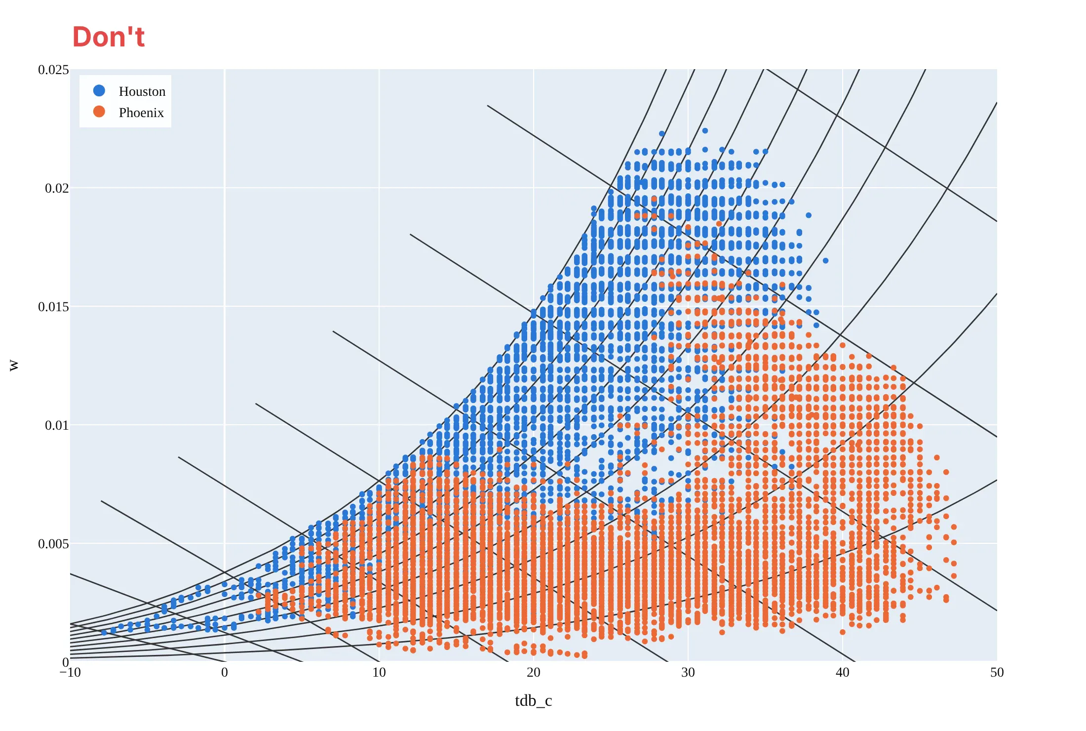
Most psychrometric charts that are hard to read bury the data under the grid, or leave out what the reader needs to trust the numbers. Here are the same Houston and Phoenix hours both ways, in the same blue and orange.

Don't draw every line family in the same dark weight so the saturation curve doesn't stand out, extend the wet-bulb lines past the saturation curve into air that can't exist, show the humidity ratio in raw kg/kg on a left axis labeled with column names ("w", "tdb_c"), use large opaque markers that hide the lines, leave the lines unlabeled, keep a serif font and a tinted background, and say nothing about the pressure:

Do keep the background lines light and the saturation curve heavy, stop every line at saturation, put the humidity ratio in g/kg on the right with a unit, label each line family where it ends (relative humidity at the right, wet bulb on the saturation curve, enthalpy on the outside scale, specific volume at the bottom), use small translucent markers, and say which pressure the lines are drawn for:

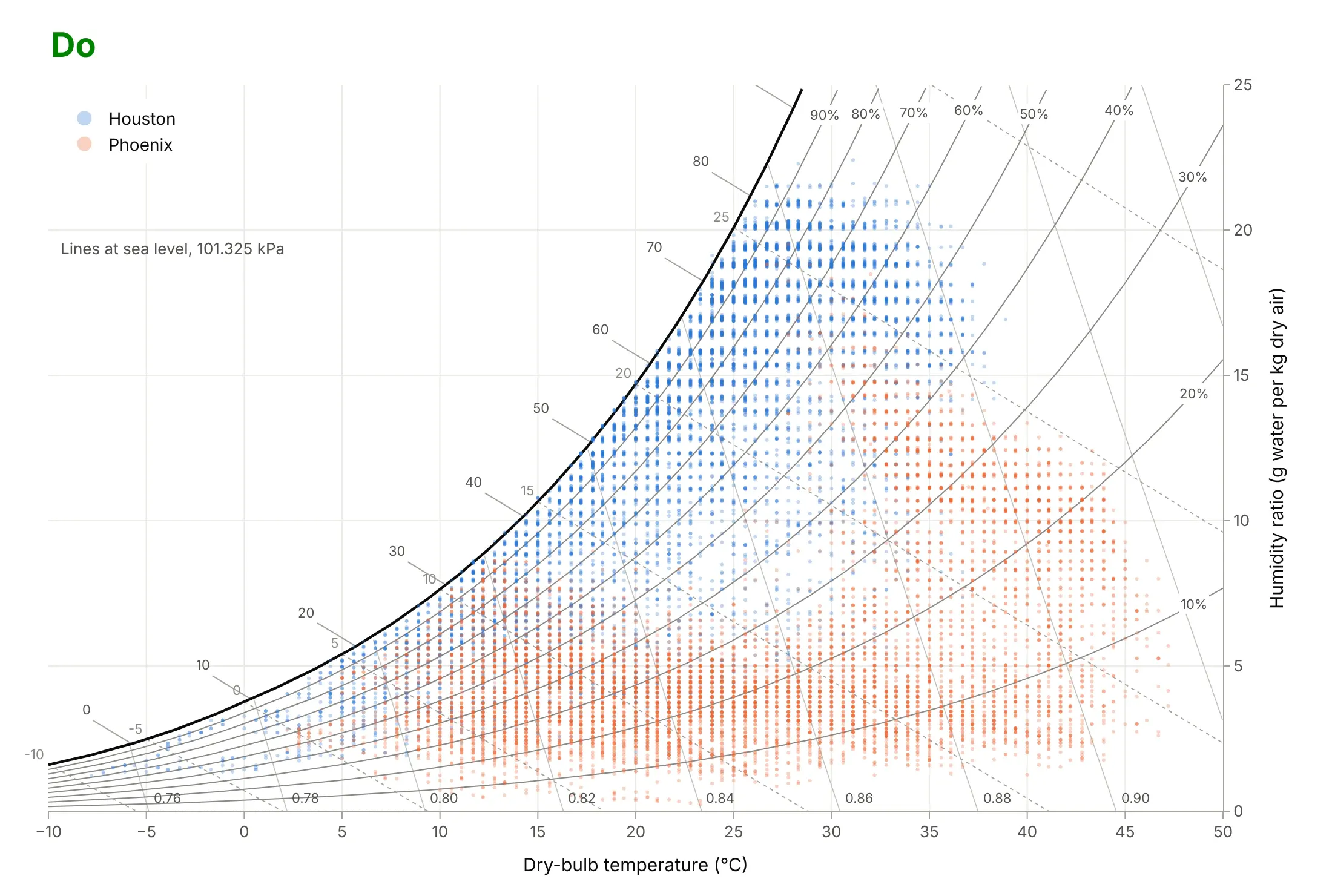
Checklist

Do

• Say which pressure (or altitude) the chart is drawn for, and draw it at the site's pressure above about 600 m.
• Put the humidity ratio on the right in g/kg (SI) or grains or pounds per pound of dry air (IP), and say "dry air".
• Draw the saturation curve heaviest, and stop every other line at it.
• Compute the lines from a tested implementation of the ASHRAE formulas, such as psychrolib, rather than by hand.
• Draw processes as arrows from the starting state, and label what is measured and what is a design choice.

Don't

• Plot relative humidity on the y axis and call it a psychrometric chart; it smears daily cycles into diagonal bands.
• Mix SI and IP units, or °C with °F, on one chart.
• Read an outdoor hour inside the comfort zone as comfortable: the zone assumes indoor air speed, clothing and activity.
• Shade the comfort zone above 12 g/kg; ASHRAE 55 asks for the full PMV calculation there.

Options to customize

A psychrometric chart in Plotly is a set of go.Scatter lines with data traces on top, so these are the options that matter most. The full lists are in the scatter trace reference, the axes documentation and the text and annotations documentation.

1. go.Scatter(mode="lines", hoverinfo="skip"): one trace per background line, so hovering only shows your data.
2. fig.update_yaxes(side="right"): the humidity ratio axis on the right, as on ASHRAE charts.
3. line=dict(width=..., dash="dot", color=...): a heavy saturation curve, light relative humidity lines, dotted wet-bulb lines.
4. go.Scattergl(mode="markers", marker=dict(size=3, opacity=0.3)): WebGL markers for a year (8,760 hours) or more of observations.
5. customdata and hovertemplate: relative humidity, dew point and wet bulb for each point in the hover.
6. go.Scatter(fill="toself"): a shaded comfort zone or design envelope from a closed polygon.
7. fig.add_annotation(x=, y=, ax=, ay=, axref="x", ayref="y", arrowhead=2): process arrows between two states in data coordinates.
8. fig.add_annotation(textangle=...) with bgcolor="white": labels on lines that stay readable over the grid.
9. fig.add_hline(y=12): a design limit such as the comfort zone's 12 g/kg cap.
10. make_subplots(rows=2, cols=3, shared_xaxes=True, shared_yaxes=True): small multiples of charts for several sites.

More psychrometric chart examples

Six more psychrometric charts, each with its source, the technique that makes it work, and a prompt to rebuild it. Three use NOAA weather data and three use indoor sensor data.

1. Denver's thin air needs its own chart

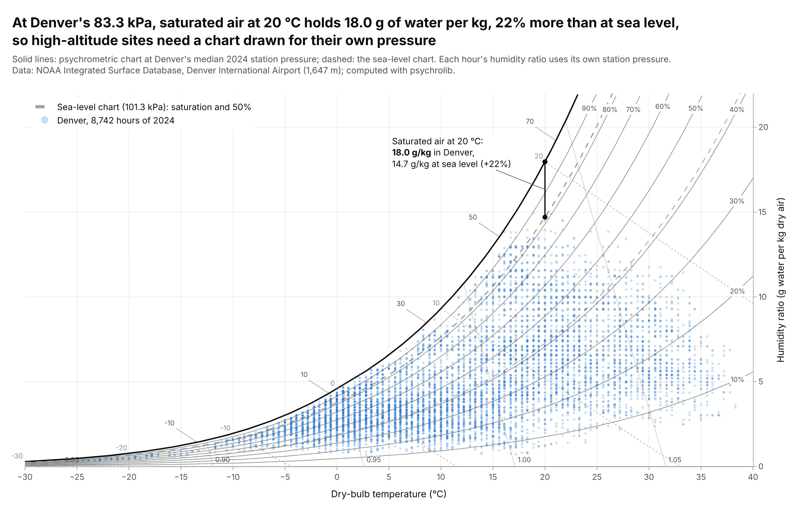
At Denver International Airport's median 2024 station pressure, 83.3 kPa, saturated air at 20 degrees C holds 18.0 g of water per kg, 22% more than the 14.7 g/kg of a sea-level chart. Reading Denver's hours against sea-level lines would put their relative humidity in the wrong place. Data: NOAA Integrated Surface Database, Denver International Airport (1,647 m), 2024.

Tip: draw the sea-level lines dashed behind the site's lines, so readers see how far the curves move.

2. Phoenix's monsoon on the wet-bulb lines

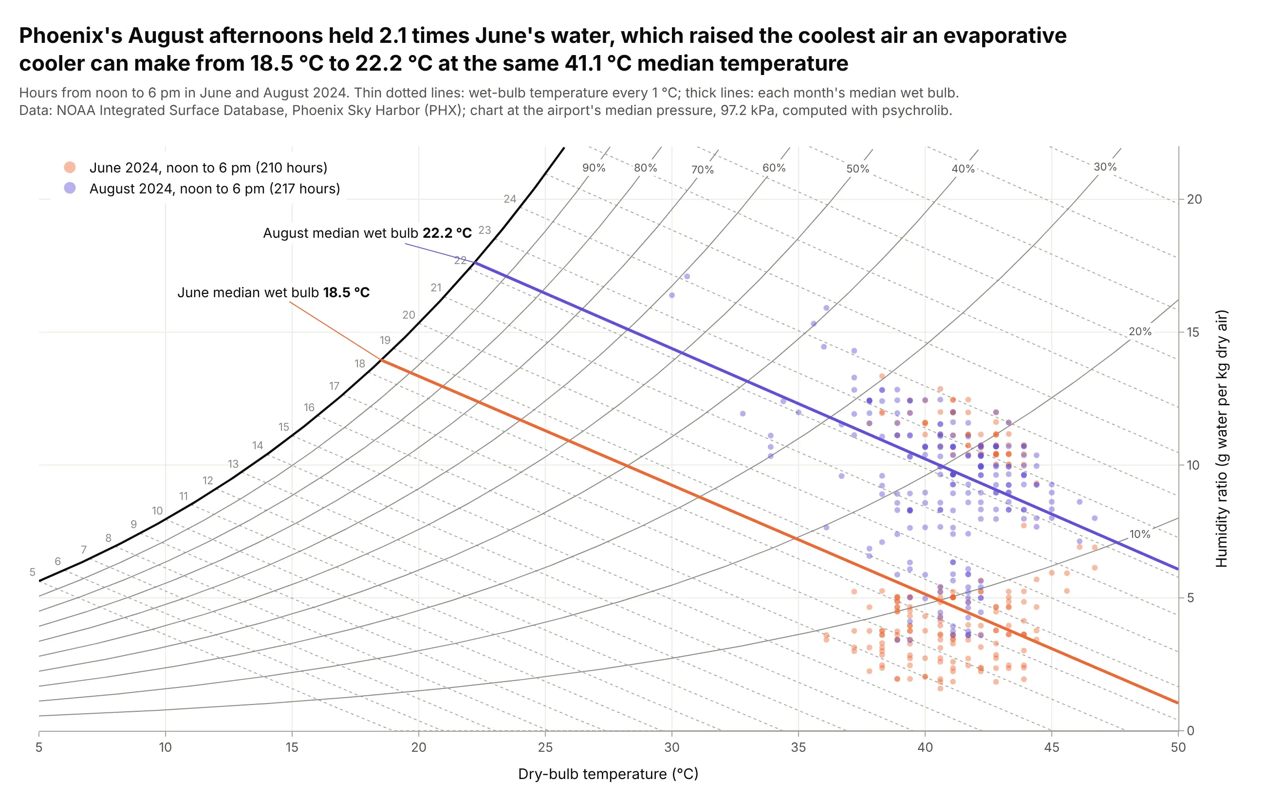
At the same 41.1 degrees C median afternoon temperature, Phoenix's August air held 2.1 times June's water, because the summer monsoon brings moist air from the south. That raised the median wet bulb, the coolest air an evaporative cooler can make, from 18.5 to 22.2 degrees C. Data: NOAA Integrated Surface Database, Phoenix Sky Harbor, June and August 2024, noon to 6 pm local time.

Tip: draw the wet-bulb lines every 1 degree, because evaporative cooling moves along them.

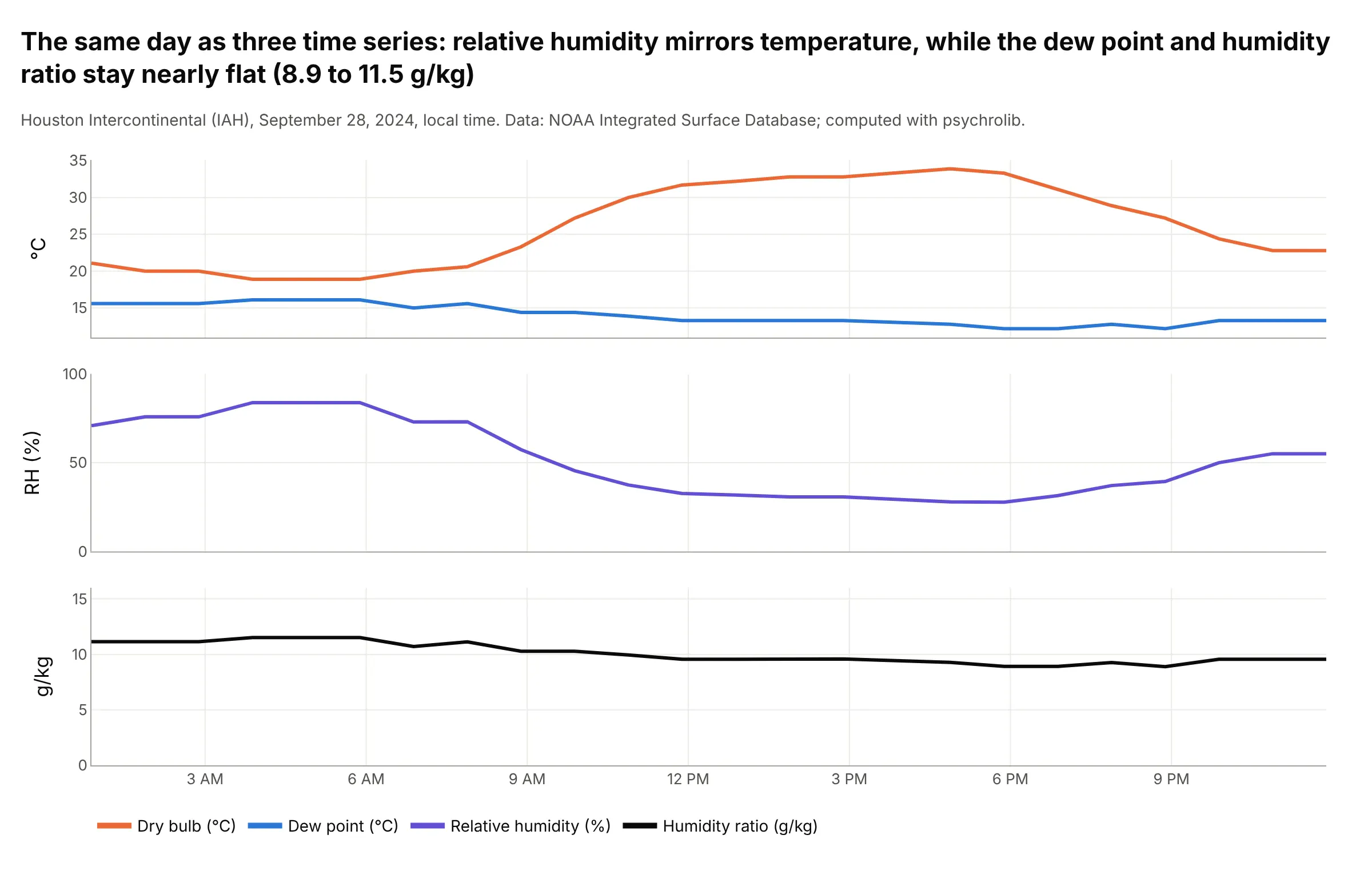
3. One day in Houston: relative humidity swings, water doesn't

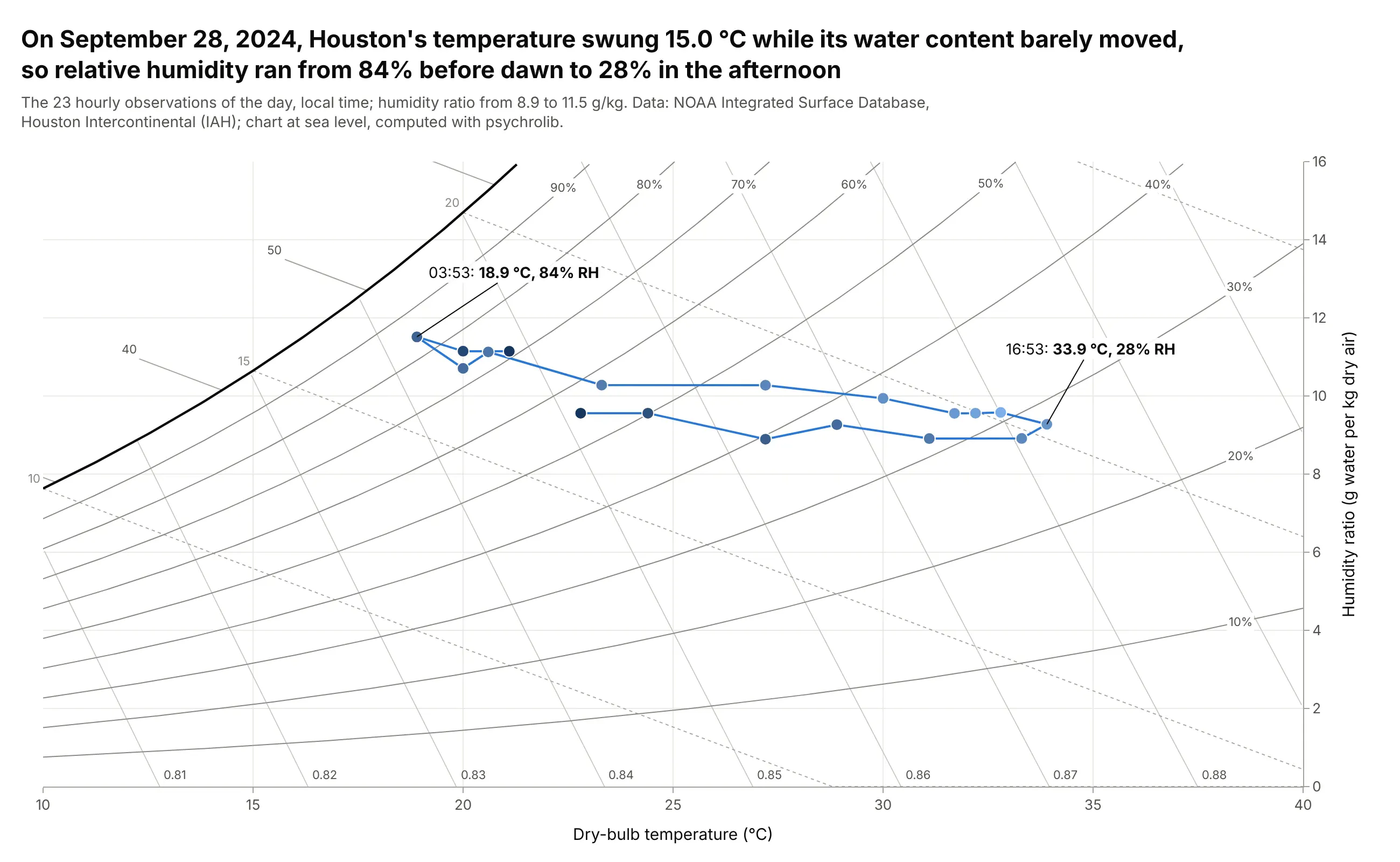
On September 28, 2024, Houston's temperature swung 15.0 degrees C, from 18.9 to 33.9, while its humidity ratio stayed between 8.9 and 11.5 g/kg, so relative humidity ran from 84% before dawn to 28% in the afternoon. On the chart, the day is a nearly flat path across the relative humidity lines. Data: NOAA Integrated Surface Database, Houston Intercontinental, local time.

Tip: join the hours in order and shade the markers from night to afternoon, so the path reads as a daily cycle.

Another way to see it: as time series, relative humidity mirrors the temperature while the dew point and humidity ratio stay nearly flat, which is the same story told hour by hour.

4. The Mollier h-x diagram, the European form

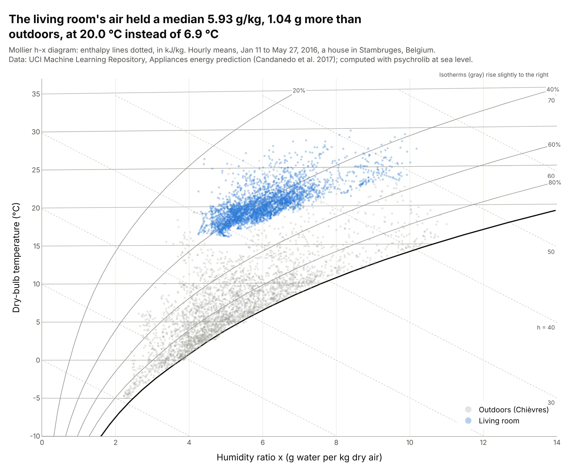
The Belgian house's living room air held a median 5.93 g/kg from January to May 2016, 1.04 g more than outdoors, at 20.0 instead of 6.9 degrees C. On a Mollier diagram, humidity ratio runs across, temperature runs up, and the enthalpy lines are straight and evenly spaced because the vertical position is enthalpy minus the latent heat of the water. Data: UCI Machine Learning Repository, Appliances energy prediction (Candanedo et al. 2017), CC BY 4.0, hourly means.

Tip: plot the vertical position as h - 2501x in kJ/kg and label its ticks in degrees C, which is how Mollier made the isotherms nearly horizontal.

5. A shower, 10 minutes at a time

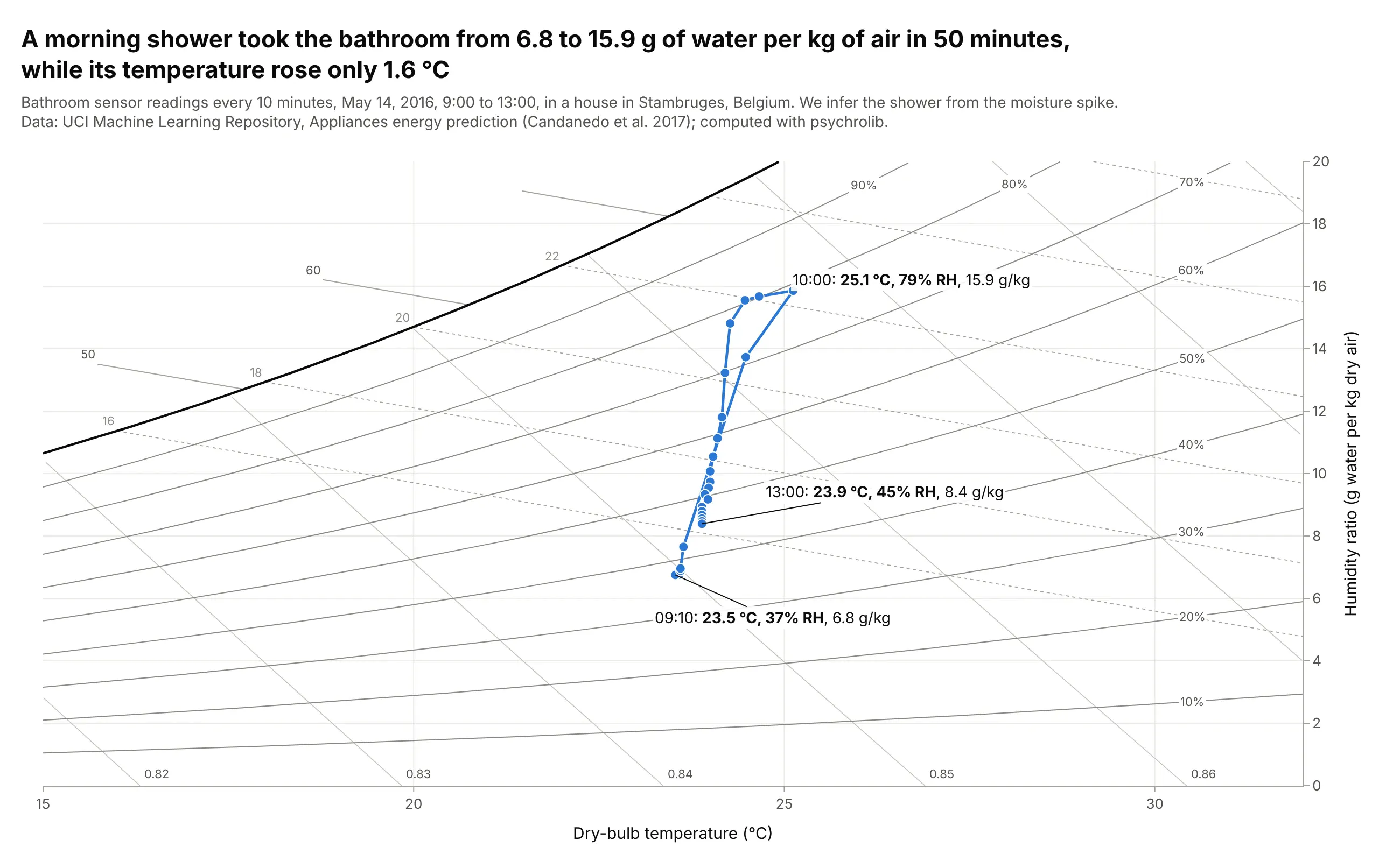
A morning shower took the bathroom from 6.8 to 15.9 g of water per kg of air in 50 minutes, while its temperature rose only 1.6 degrees C, from 23.5 to 25.1. Adding water at a nearly constant temperature is a vertical move on the chart, and ventilation brought it back down to 8.4 g/kg by 13:00. Data: UCI Machine Learning Repository, Appliances energy prediction (Candanedo et al. 2017), CC BY 4.0; we infer the shower from the moisture spike.

Tip: label the before, peak and after states with time, temperature, relative humidity and humidity ratio.

6. People add water to a dry winter office

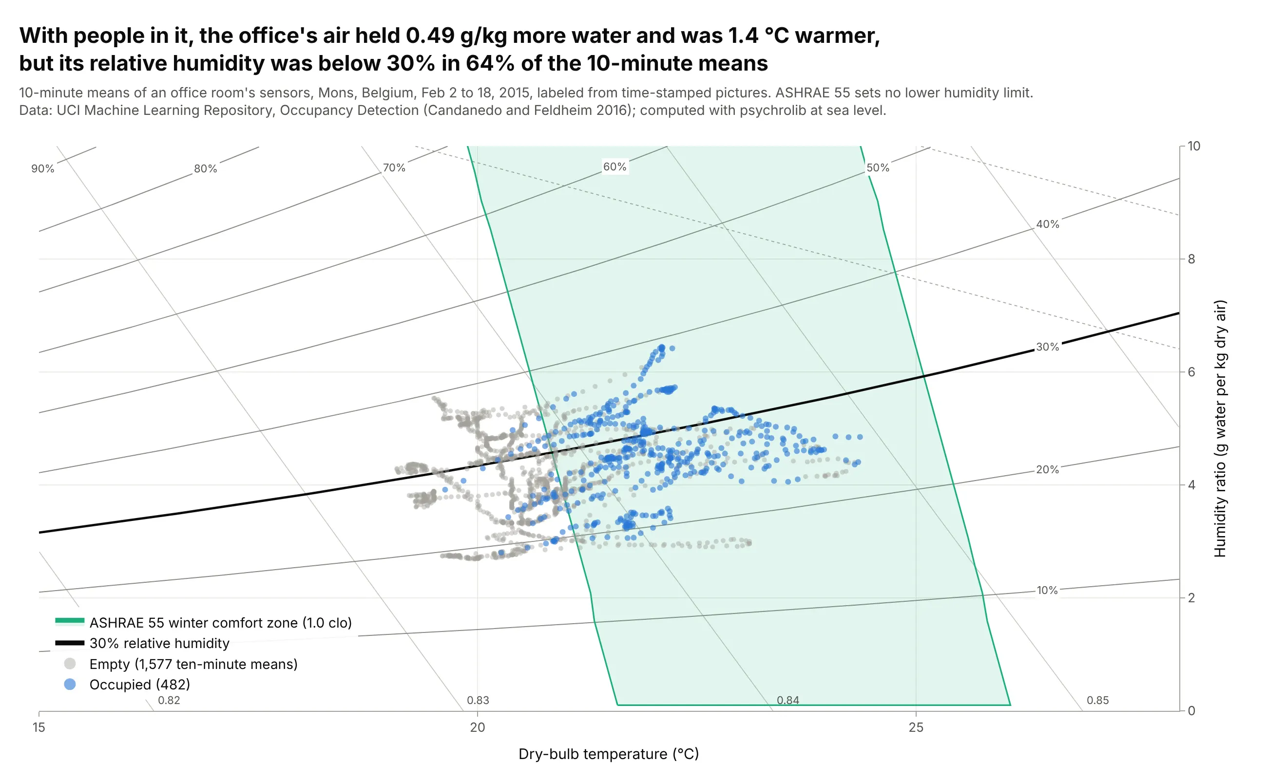
With people in it, the office's air held a median 0.49 g/kg more water and was 1.4 degrees C warmer than when it was empty, since people breathe out water vapor and give off heat. Its relative humidity was below 30% in 64% of the 10-minute means, typical of heated winter air, and ASHRAE 55 sets no lower humidity limit. Data: UCI Machine Learning Repository, Occupancy Detection (Candanedo and Feldheim 2016), CC BY 4.0, February 2 to 18, 2015.

Tip: draw the one relative humidity line your readers care about in black, here 30%.