Chris Parmer

November 3, 2026

Smith Charts - A Complete Guide

TL;DR

A Smith chart plots impedance, or a measured reflection coefficient such as S11, inside a circle: the center is a perfect 50 ohm match, the outer edge is total reflection, and a sweep across frequency draws a curve.
Smith charts are also known as Smith diagrams, impedance charts and Volpert-Smith charts, and are similar to a polar chart of the reflection coefficient, with a grid of resistance circles and reactance arcs printed on top.
RF and microwave engineers use them to match antennas, design amplifier and filter matching networks, and read S-parameters from a vector network analyzer.
You can make a Smith chart with Plotly in Python or JavaScript with the built-in scattersmith trace, which takes the impedance normalized to 50 ohms through real and imag.

What is a Smith chart?

Smith charts look like this:

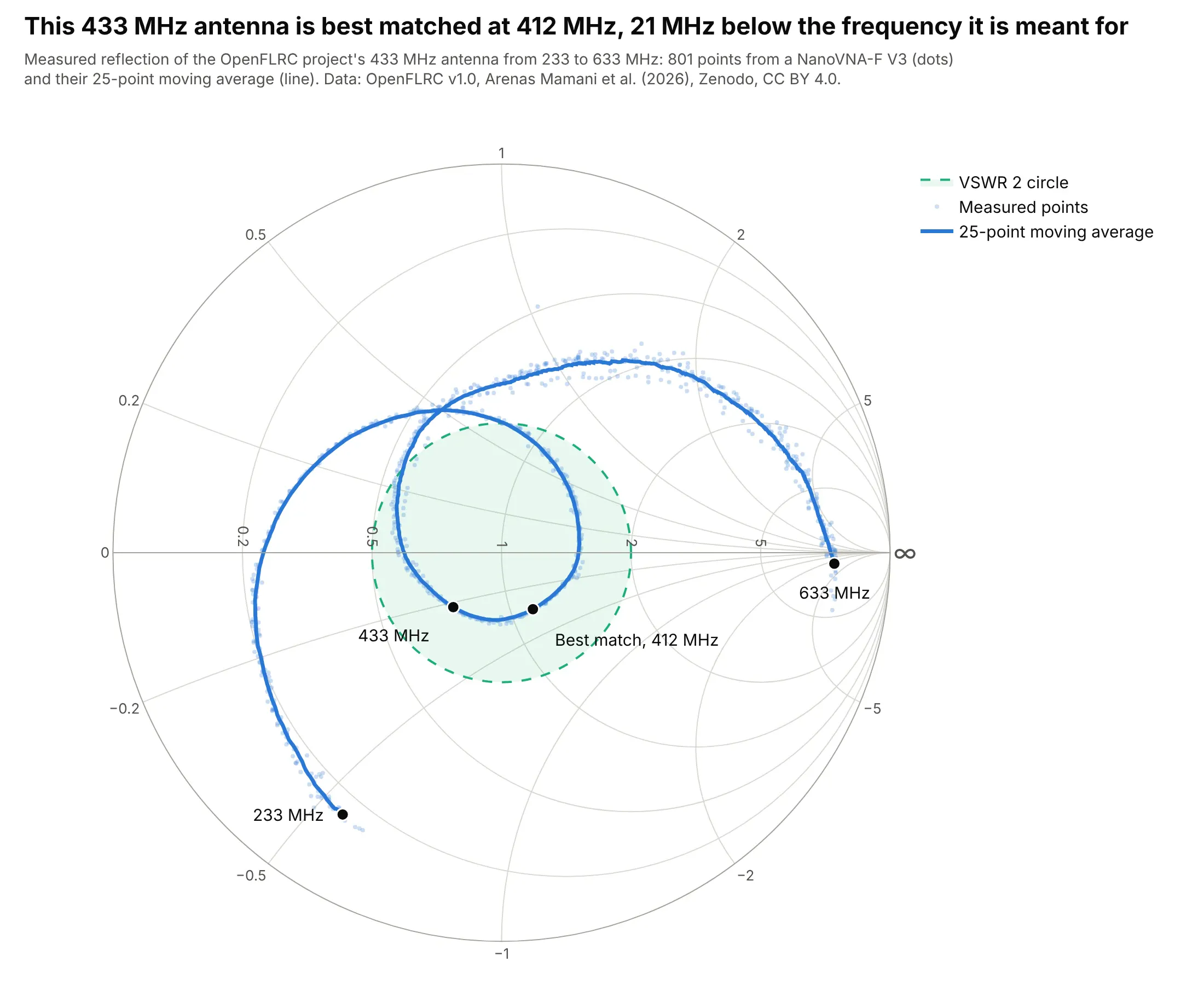
Smith chart of a 433 MHz antenna's measured reflection from 233 to 633 MHz: a curve that starts in the lower left near the edge, loops once inside a green VSWR 2 circle around the center, and ends near the open-circuit point on the right; the best match is marked at 412 MHz and 433 MHz is marked just beside it

Data: OpenFLRC v1.0, Arenas Mamani et al. (2026), Zenodo, CC BY 4.0, measured with a NanoVNA-F V3.

How do you read a Smith chart? In the example above, notice these things:

Every point is the antenna's impedance at one frequency, and the curve runs from 233 MHz (lower left) to 633 MHz (near the right edge, close to an open circuit).
The closer a point is to the center, the better the match to 50 ohms. The best match is at 412 MHz, where the antenna takes 97.2% of the power, and at 433 MHz it takes 96.5%.
The green circle is VSWR 2, a common pass mark. The curve is inside it from 347 to 468 MHz, a 120 MHz wide band.
Points above the horizontal line are inductive and points below are capacitive. At 433 MHz the antenna is 38 - j11 ohms, a little low in resistance and slightly capacitive, which tells whoever tunes it which way to move.
The faint dots are the 801 raw points from a low-cost analyzer; the line is a 25-point moving average, so the noise doesn't hide the shape.

It's often used for charts like these:

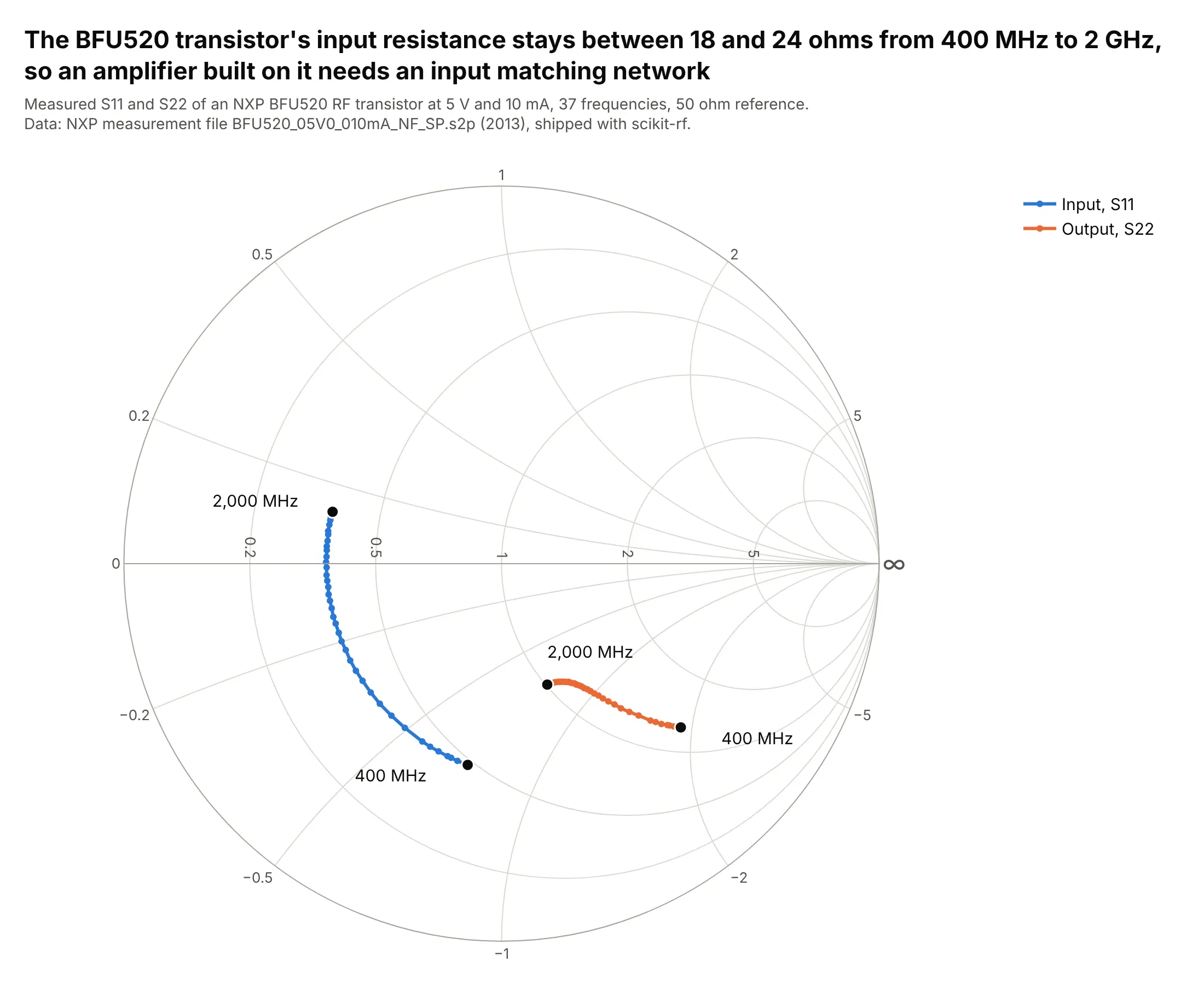
Smith chart of an NXP BFU520 transistor's measured S11 and S22 from 400 to 2,000 MHz: the input curve sits on the left at low resistance and the output curve in the lower middle, both with their end frequencies labeled

Amplifier S-parameters. The BFU520 transistor's input resistance stays between 18 and 24 ohms from 400 MHz to 2 GHz, so an amplifier built on it needs a matching network before 50 ohm parts can drive it. Data: NXP measurement file, shipped with scikit-rf (BSD-3-Clause).

Smith chart of a Mini-Circuits LFCN-2352+ low-pass filter's input reflection from 10 MHz to 50 GHz: a blue knot around the center for the passband and orange loops out near the edge for the stopband, with the -3 dB point at 24.9 GHz marked

Filters. The LFCN-2352+ low-pass filter's input stays close to 50 ohms, within -14 dB of reflection, up to 20 GHz and passes signals up to 24.9 GHz; above that its impedance swings out toward the edge as it blocks. Data: Mini-Circuits S-parameter file, shipped with scikit-rf.

How to read the circles on a Smith chart

A Smith chart is a map of every possible impedance squeezed into one circle. Read it like latitude and longitude on a globe: every point sits on exactly one resistance circle and one reactance arc, and the pair of values is the impedance.

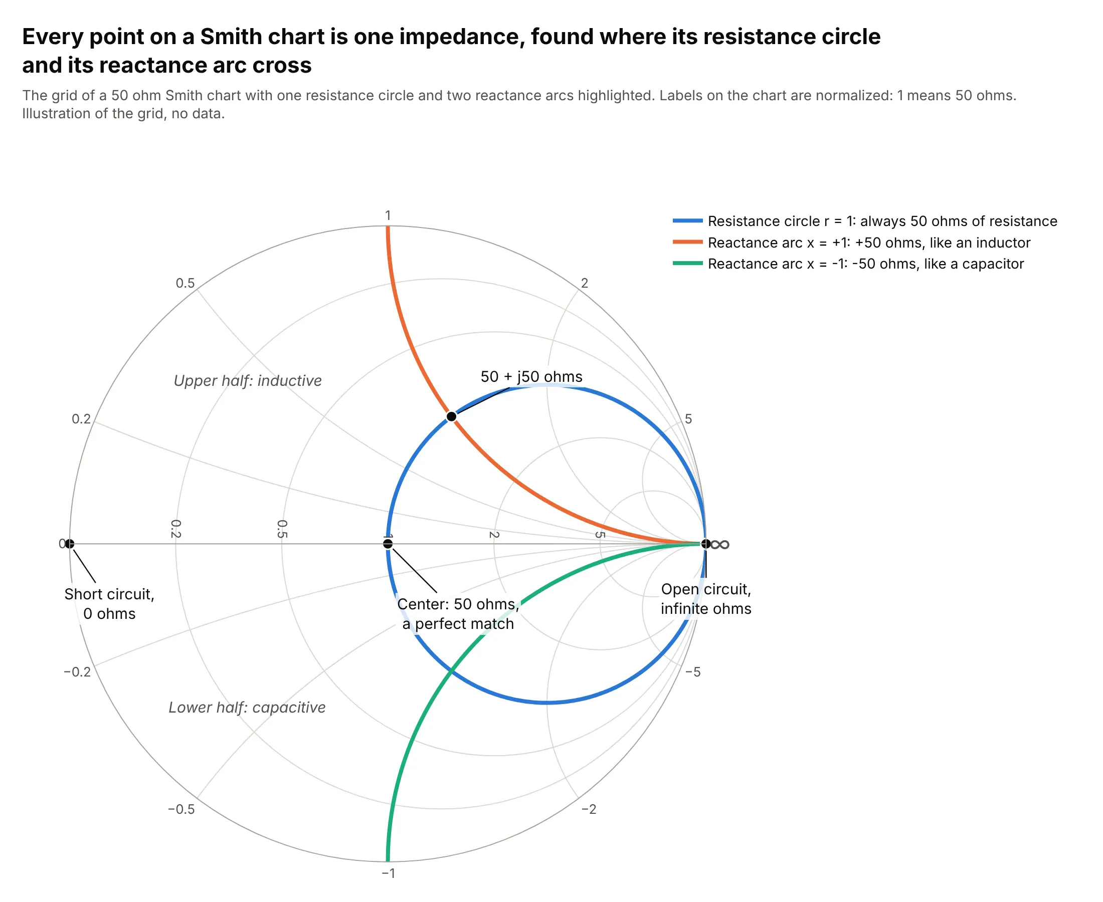
A Smith chart grid with the r = 1 resistance circle in blue, the x = +1 reactance arc in orange and the x = -1 arc in green, crossing at 50 + j50 ohms, with the short circuit at the left end, the open circuit at the right end and the 50 ohm center labeled

Resistance circles all touch the right edge. Every point on one has the same resistance, and bigger resistances are smaller circles further right. The circle through the center is 50 ohms.
Reactance arcs fan out from the same right-hand point. Every point on one has the same reactance: arcs in the upper half are inductive (positive), arcs in the lower half capacitive (negative), and the straight horizontal line is zero reactance, a pure resistor.
The landmarks: the left end of the horizontal line is a short circuit (0 ohms), the right end an open circuit, the center a perfect match, and the outer circle pure reactance, where everything is reflected.
The labels are normalized: 1 means the reference impedance, usually 50 ohms, so 2 means 100 ohms and 0.5 means 25 ohms.
Distance from the center is the reflection. Circles centered on the middle are constant VSWR (or return loss), which is why a "VSWR 2 circle" works as a target.

A short history

Phillip H. Smith of Bell Telephone Laboratories published the chart as a "Transmission Line Calculator" in Electronics in January 1939 (Smith 1939, vol. 12, no. 1, pp. 29-31), as a way to solve transmission-line problems "without recourse to lengthy computations". Tosaku Mizuhashi (1937) and Amiel R. Volpert (1939) proposed the same chart independently (Wikipedia), and Smith published an improved version in 1944 (Smith 1944). This is the worked example from his 1939 article, redrawn:

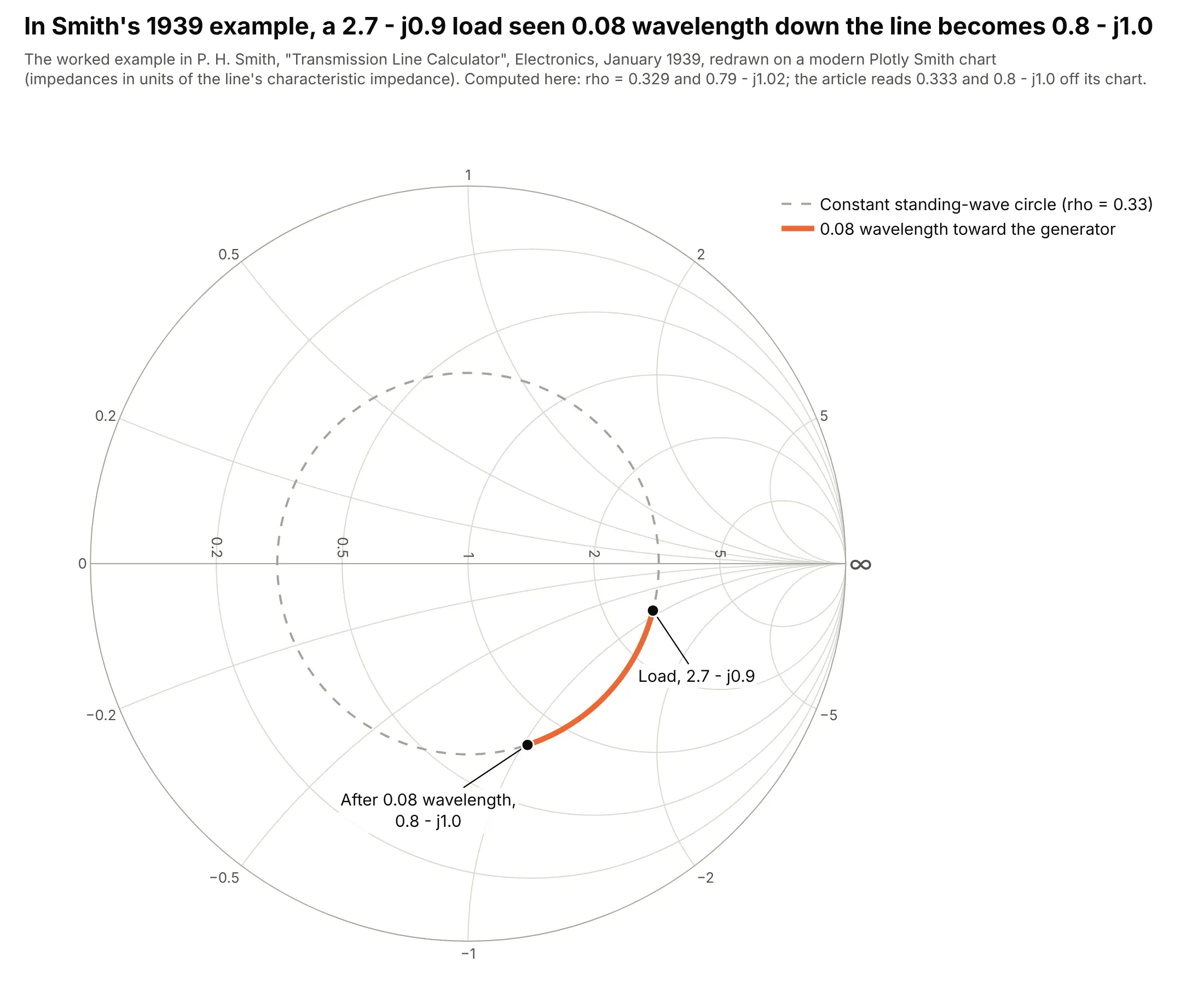
Smith's 1939 worked example redrawn on a Plotly Smith chart: a load of 2.7 - j0.9 on a dashed circle of constant standing-wave ratio, and an orange arc 0.08 wavelength clockwise to 0.8 - j1.0

Data: P. H. Smith, "Transmission Line Calculator", Electronics, January 1939, worked example (text checked through RF Cafe's reproduction).

A load of 2.7 - j0.9 times the line's impedance sits on the circle Smith marked 0.333, his ratio of minimum to maximum voltage. Moving 0.08 wavelength toward the generator turns the point around that circle to 0.8 - j1.0, which is the whole trick: walking along a line only rotates the impedance around the center.

Alternatives to a Smith chart

Here's the same 433 MHz antenna measurement drawn six ways. Some are better for the question, some worse, some just different:

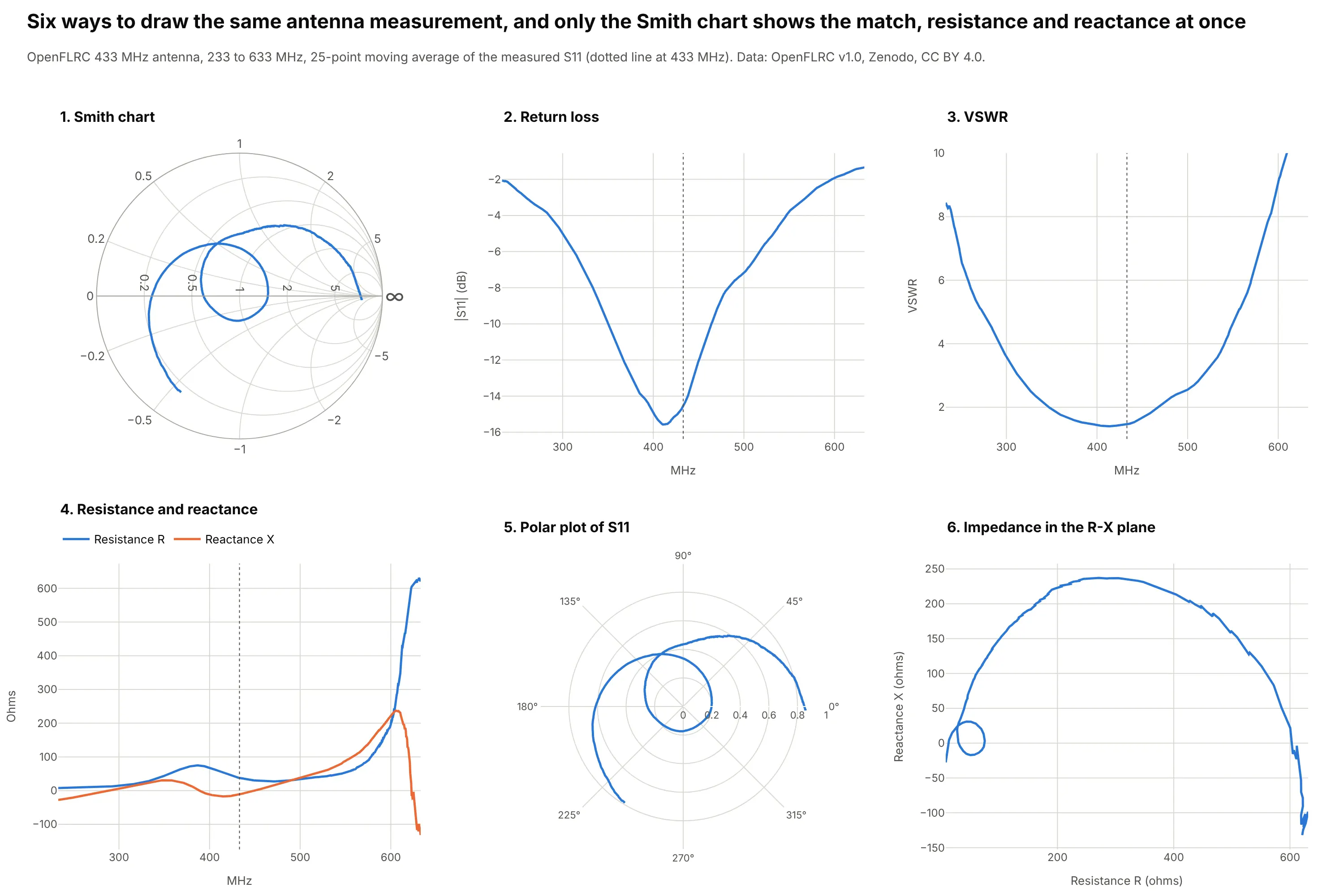
Six charts of the same 433 MHz antenna sweep: a Smith chart, |S11| in dB against frequency with a dip at 412 MHz, VSWR against frequency, resistance and reactance in ohms against frequency, a polar plot of S11 that has the same shape as the Smith chart without its grid, and the impedance as a path in the resistance-reactance plane that runs out to 600 ohms

Return loss, |S11| in dB (better for the bandwidth). The dip at 412 MHz and the band below -10 dB are easy to read off the axis, which is why datasheets use it, but it can't tell a too-high resistance from a too-low one, or inductive from capacitive.
VSWR against frequency (works too). The same information as return loss on a different scale, common for antennas and transmitters.
Resistance and reactance against frequency (works too, for impedance in ohms). Two lines give the exact impedance at every frequency, but the near-open-circuit end shoots up to 600 ohms and squashes the interesting part.
Polar plot of S11 (different). It's the Smith chart without the grid: the same curve, but you can't read off ohms.
Impedance in the resistance-reactance plane (worse). The same path as the Smith chart on a flat grid, where high impedances take over the plot and the matched region near 50 ohms is a tiny loop.

How to make a Smith chart

With AI

ChatGPT, Claude Code, GitHub Copilot, Cursor and other AI tools are excellent at writing Plotly code. Name Plotly in the prompt, say what's in your Touchstone file and remind it that the trace takes impedance, not S11:

Make a plotly Smith chart from antenna.s1p (a Touchstone file of measured S11 in a 50 ohm system).

- Read it with scikit-rf, convert S11 to normalized impedance z = (1 + S11) / (1 - S11) and plot
  go.Scattersmith(real=z.real, imag=z.imag).
- Add a 25-point moving average of S11 as the main line and the raw points as faint dots.
- Draw a dashed VSWR 2 circle, mark and label the best match and 433 MHz, frequency in the hover text.
- Inter font, fixed size, a title that states the takeaway with the best-match frequency.
- Check: print the best-match frequency, its VSWR and the band where VSWR is below 2.

With Plotly Studio

Plotly Studio is a desktop app where you point an AI at a dataset and it builds charts and a Dash app around your questions. Ask for a Smith chart the same way:

Show the antenna's measured S11 on a Smith chart from 233 to 633 MHz, with a VSWR 2 circle, the best match labeled, and a slider to pick a frequency and read its impedance in ohms.

Make a Smith chart in Python or JavaScript

This is the code AI tools write under the hood. In Python, go.Scattersmith draws the chart and scikit-rf reads the Touchstone file; the Plotly Smith chart documentation covers subplots and styling:

import plotly.graph_objects as go
import skrf as rf  # pip install scikit-rf; reads Touchstone (.s1p, .s2p) files

ntwk = rf.Network("antenna.s1p")
s11 = ntwk.s[:, 0, 0]
z = (1 + s11) / (1 - s11)  # Scattersmith takes impedance normalized to 50 ohms, not S11

fig = go.Figure(go.Scattersmith(
    real=z.real, imag=z.imag, mode="lines", customdata=ntwk.f / 1e6,
    hovertemplate="%{customdata:.0f} MHz: z = %{real:.2f} %{imag:+.2f}j<extra></extra>"))
fig.show()

real and imag are resistance and reactance divided by the reference impedance, so 1 is 50 ohms. If you already have impedances in ohms, divide by 50; if you have S11, convert it as above.

In JavaScript, plotly.js has the same scattersmith trace:

<div id="chart"></div>
<script src="https://cdn.plot.ly/plotly-4.1.1.min.js"></script>
<script>
  // NXP BFU520 transistor, measured S11 (magnitude, angle in degrees) at 5 V, 10 mA
  const mhz = [400, 600, 900, 1200, 1600, 2000];
  const mag = [0.54054, 0.49714, 0.47167, 0.46475, 0.46403, 0.46792];
  const deg = [-99.54, -125.91, -150.99, -167.79, 175.60, 162.95];

  // Scattersmith takes normalized impedance z = (1 + S11) / (1 - S11)
  const z = mag.map((m, i) => {
    const gr = m * Math.cos(deg[i] * Math.PI / 180), gi = m * Math.sin(deg[i] * Math.PI / 180);
    const d = (1 - gr) ** 2 + gi ** 2;
    return {r: (1 - gr * gr - gi * gi) / d, x: 2 * gi / d};
  });

  Plotly.newPlot("chart", [{
    type: "scattersmith", mode: "lines+markers",
    real: z.map(p => p.r), imag: z.map(p => p.x),
    text: mhz.map(f => f + " MHz"), hovertemplate: "%{text}: z = %{real:.2f} %{imag:+.2f}j<extra></extra>",
    line: {color: "#2a78d6", width: 3}
  }], {width: 600, height: 600, font: {family: "Inter, Arial, sans-serif"}});
</script>

Share it

Every Plotly chart has a Share chart button (the cloud icon in its toolbar) that uploads it to Plotly Cloud and gives you a link. Only you can see it until you change its visibility.

For a live app, put the chart in a Dash app and publish it with the Plotly Cloud CLI. Coding agents can run these commands for you:

pip install "dash[cloud]"
plotly user login
plotly app publish

If your data has to stay in your own cloud or data center, publish to Dash Enterprise instead.

Dos and don'ts

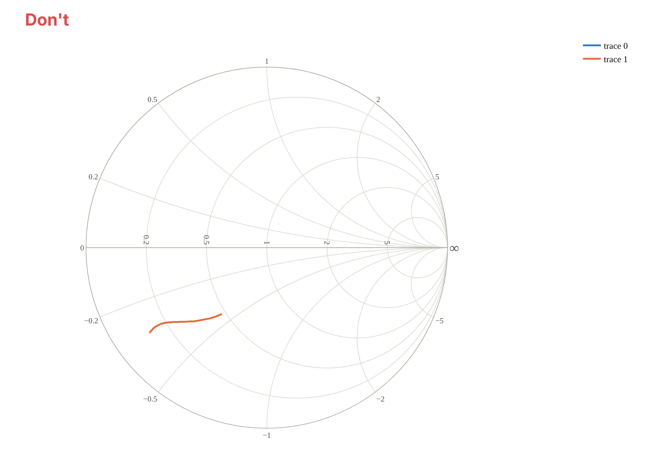
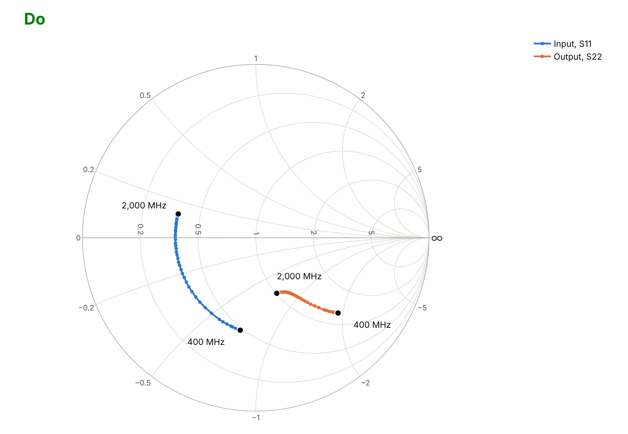
Most Smith chart mistakes come from what goes into the trace, not how it's styled. Here is the BFU520 transistor's input and output both ways, in the same colors.

Don't pass S11's real and imaginary parts straight to real and imag, leave the default trace names, skip the frequency labels or use a default serif font. Scattersmith reads those numbers as resistance and reactance, so the input trace, whose real part is negative at every frequency, disappears without an error, and the output lands in the wrong place:

A Smith chart with a legend of trace 0 and trace 1 in a serif font, where only one short orange curve appears in the lower left and the blue input trace is missing

Do convert to normalized impedance with z = (1 + S11) / (1 - S11), name the traces, put markers on the measured frequencies and label where each sweep starts and ends:

The same transistor drawn correctly: a blue input curve on the left and an orange output curve in the lower middle, named Input, S11 and Output, S22, with 400 and 2,000 MHz labeled on each

Checklist

Convert S-parameters to normalized impedance before plotting, and say which reference impedance (usually 50 ohms) you used.
Label the start and end frequency, or color by frequency, so readers know which way the sweep runs.
Put the frequency in the hover text with customdata and hovertemplate.
Add a VSWR or return-loss circle when the question is "is it matched?".
Smooth noisy measurements, and show the raw points faintly behind the line.
Pair the chart with a dB plot when the curve is a small knot around the center.

Don't

Use a Smith chart for transmission terms like S21; plot those in dB against frequency.
Overload one chart with many ports and many frequencies; split them into subplots.
Read ohms off the labels without multiplying by the reference impedance.

Options to customize

These are the options that matter most for a Smith chart in Plotly. The full lists are in the scattersmith reference and the layout.smith reference.

real, imag: normalized resistance and reactance (impedance divided by the reference); points with negative resistance are not drawn.
mode: "lines" for dense sweeps, "lines+markers" to show each measured frequency, "text" for labels at an impedance.
customdata with hovertemplate: frequency, ohms or VSWR in the hover text.
marker.color with colorscale: color the points by frequency, with a colorbar.
fill="toself": shade a region, such as a VSWR circle or an unstable area.
subplot="smith2" and layout.smith2.domain: several Smith charts in one figure, side by side.
layout.smith.domain: place a Smith chart next to ordinary axes, like a return-loss plot.
realaxis.tickvals, imaginaryaxis.tickvals: which resistance circles and reactance arcs the grid shows.
realaxis.gridcolor, imaginaryaxis.gridcolor, bgcolor: a lighter grid so the data stands out.
fig.update_smiths(...): style every Smith subplot at once.

More Smith chart examples

Seven more Smith charts from measured data, each with its source, the technique that makes it work and a prompt to rebuild it. They cover the textbook uses: transmission lines, antennas, matching networks, noise and stability circles, multiport components and temperature drift.

1. An open-ended microstrip line

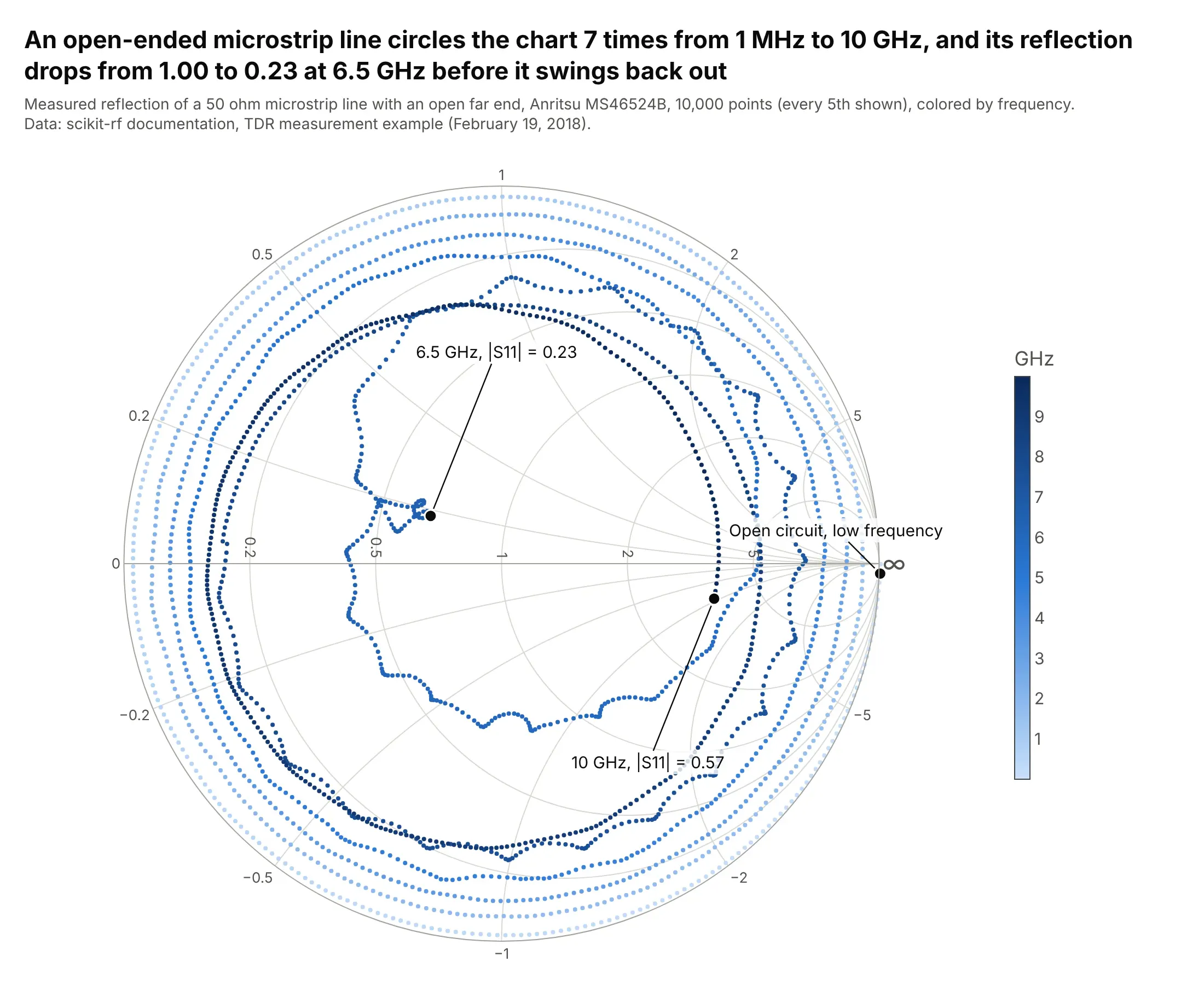
Smith chart of an open-ended 50 ohm microstrip line measured from 1 MHz to 10 GHz, colored from light blue at low frequency to dark blue at high frequency: rings that circle the chart seven times starting at the open-circuit point, with one deep loop to |S11| = 0.23 at 6.5 GHz and |S11| = 0.57 at 10 GHz

Moving along a transmission line rotates the impedance around the chart, one full turn per half wavelength, so this open-ended line circles the chart 7 times between 1 MHz and 10 GHz. Its reflection drops from 1.00 to 0.23 at 6.5 GHz before swinging back out. Data: scikit-rf documentation, TDR measurement example (Anritsu MS46524B, February 19, 2018).

Tip: color the points by frequency with a colorscale when a sweep crosses itself, so readers can follow it.

Get the data from scikit-rf's documentation, the measured one-port file P1-MSL_Open_50.s1p in
doc/source/examples/networktheory/tdr_measurement_vs_simulation/measurement (a 50 ohm microstrip line with an
open end, 1 MHz to 10 GHz), and shape it into a table (columns: freq_mhz, gamma_re, gamma_im).

Build a plotly Smith chart with go.Scattersmith: convert to z = (1 + S11) / (1 - S11), every 5th point as
4 px markers colored by frequency with a colorbar, and the start, the lowest |S11| and the 10 GHz point labeled.

2. Two antennas, two bands

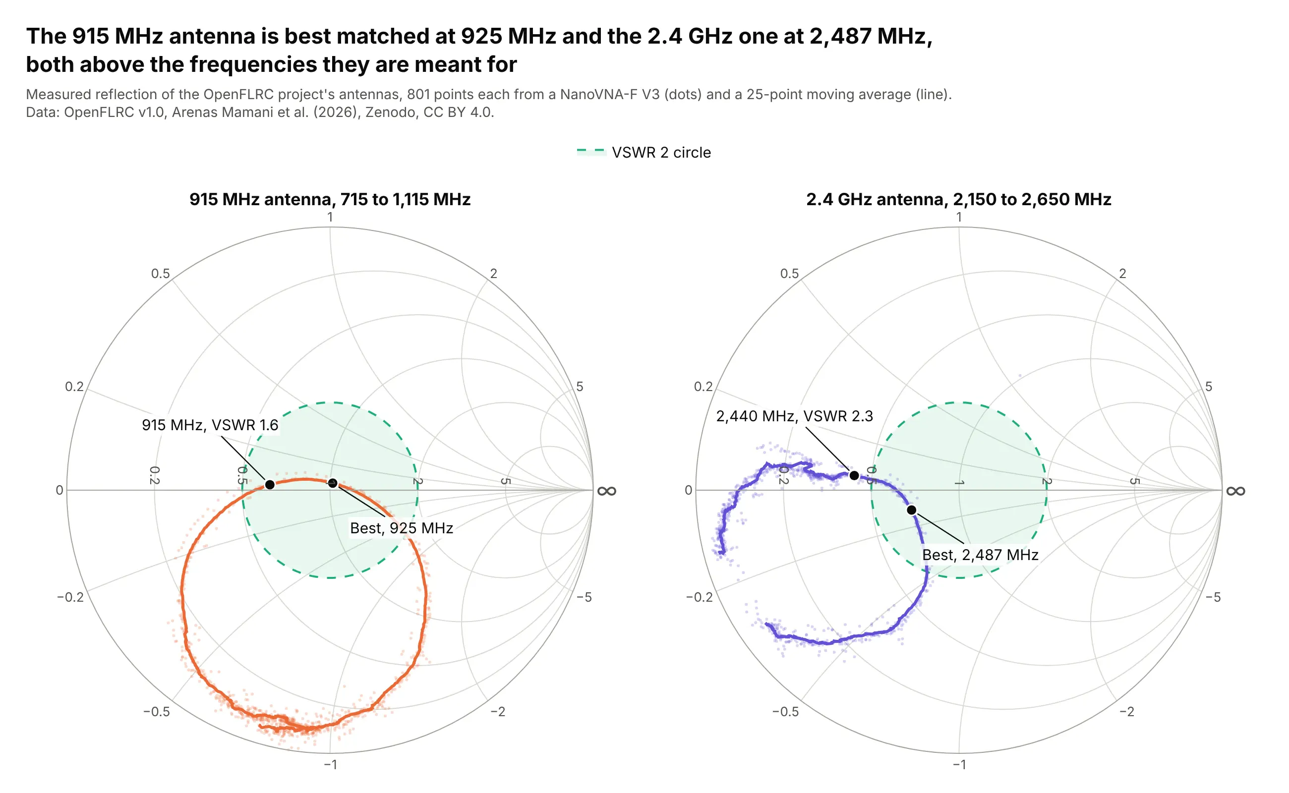
Two Smith charts side by side for the 915 MHz and 2.4 GHz antennas, each with raw dots, a moving-average line and a green VSWR 2 circle; the 915 MHz antenna's best match is at 925 MHz and the 2.4 GHz one's at 2,487 MHz, with VSWR 1.6 at 915 MHz and 2.3 at 2,440 MHz

The same project's 915 MHz antenna is best matched at 925 MHz and its 2.4 GHz antenna at 2,487 MHz, so both are tuned slightly high. At 2,440 MHz the 2.4 GHz antenna's VSWR is 2.3, outside the VSWR 2 circle. Data: OpenFLRC v1.0, Zenodo, CC BY 4.0.

Tip: give each antenna its own Smith subplot with the same VSWR circle, rather than overlaying curves that cross.

Get the data from the OpenFLRC v1.0 dataset on Zenodo (doi 10.5281/zenodo.21159006, CC BY 4.0), the NanoVNA
sweeps 21_09_30.s1p and 21_17_55.s1p in measurements/phase4_antenna_characterisation, and shape them into a
table (columns: antenna, freq_mhz, gamma_re, gamma_im).

Build two plotly Smith charts side by side (subplot "smith" and "smith2"): raw points faint, a 25-point moving
average as the line, a dashed VSWR 2 circle, and the best match and the operating frequency labeled on each.

3. An L-network matching the transistor's input

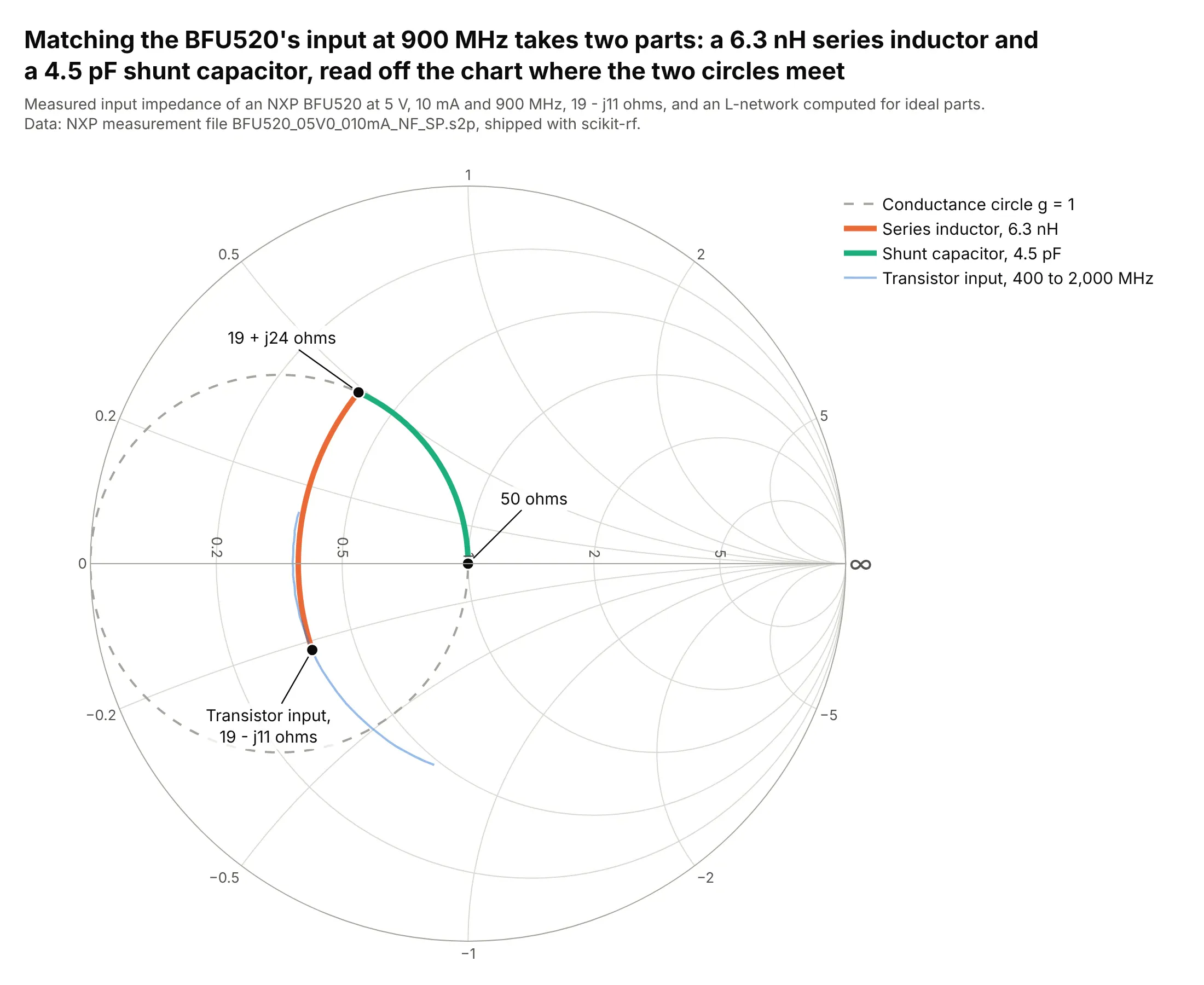
Smith chart of the BFU520's input at 900 MHz, 19 - j11 ohms, with an orange arc up its constant-resistance circle to 19 + j24 ohms on a dashed unit conductance circle, then a green arc along that circle to the 50 ohm center

Matching the BFU520's input at 900 MHz takes a 6.3 nH series inductor and a 4.5 pF shunt capacitor, read off the chart where the constant-resistance circle meets the unit conductance circle. The values are computed for ideal parts from the measured input impedance. Data: NXP measurement file, shipped with scikit-rf.

Tip: Plotly's grid draws impedance circles, so draw the admittance (conductance) circle you need as an extra dashed trace with z = 1 / (g + jb).

Get the data from scikit-rf's documentation, the NXP file BFU520_05V0_010mA_NF_SP.s2p (measured S-parameters
of a BFU520 transistor at 5 V and 10 mA, 400 to 2,000 MHz), and shape it into a table (columns: freq_mhz,
param, gamma_re, gamma_im).

Build a plotly Smith chart that designs an L-network at 900 MHz: the S11 point, a series-inductor arc along
its constant-resistance circle to the g = 1 circle, a shunt-capacitor arc to the center, the g = 1 circle
dashed, and the inductor and capacitor values in the legend.

4. Noise figure circles

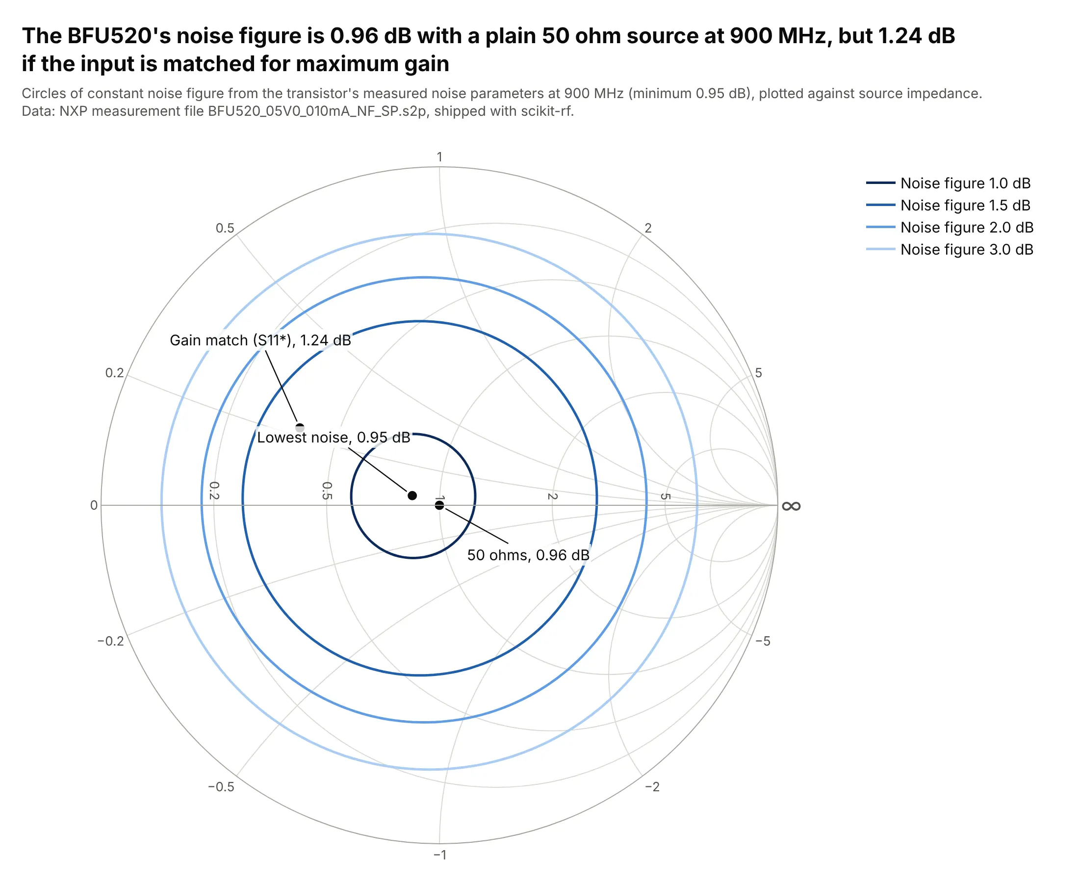
Smith chart of four nested blue circles of constant noise figure, 1.0, 1.5, 2.0 and 3.0 dB, around the BFU520's lowest-noise point near the center, with 50 ohms marked at 0.96 dB and the gain-match point marked at 1.24 dB

At 900 MHz the BFU520's noise figure is 0.96 dB with a plain 50 ohm source, almost its 0.95 dB minimum, but 1.24 dB if the input is matched for maximum gain. The circles come from the transistor's measured noise parameters. Data: NXP measurement file, shipped with scikit-rf; textbook noise-circle formulas (as in Pozar, Microwave Engineering).

Tip: draw computed circles as ordinary Scattersmith line traces in one hue, darker for the better values.

Get the data from scikit-rf's documentation, the NXP file BFU520_05V0_010mA_NF_SP.s2p, and shape its noise
block into a table (columns: freq_mhz, nfmin_db, gopt_re, gopt_im, rn_norm) and its S-parameters into another
(columns: freq_mhz, param, gamma_re, gamma_im).

Build a plotly Smith chart of constant noise figure circles at 900 MHz for 1.0, 1.5, 2.0 and 3.0 dB, with
the optimum source, 50 ohms and the conjugate of S11 marked and their noise figures labeled.

5. Stability circles

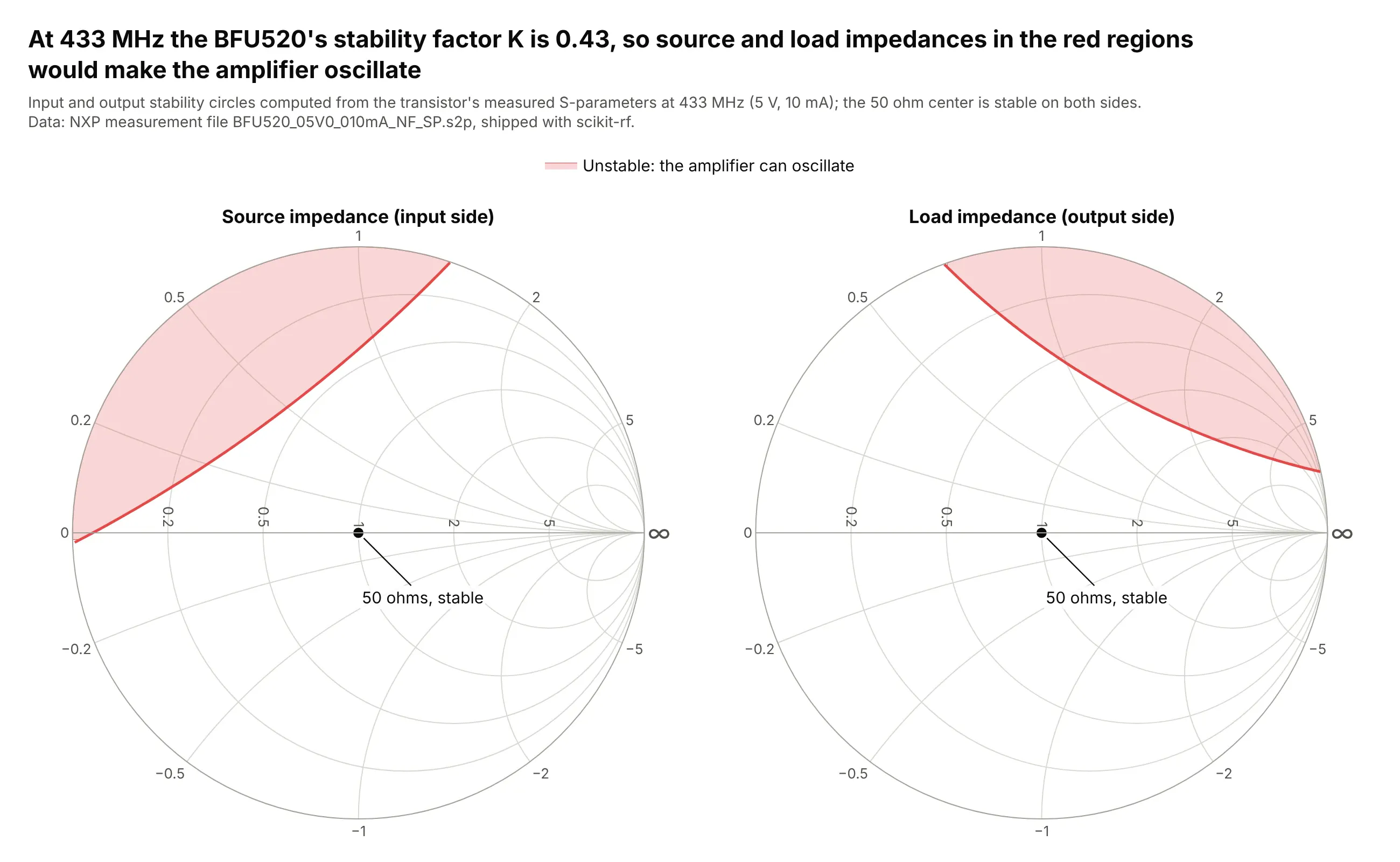
Two Smith charts for the source and load sides of the BFU520 at 433 MHz, each with a red shaded region at the top edge marking impedances that would make the amplifier oscillate, and the 50 ohm center marked as stable

At 433 MHz the BFU520's stability factor K is 0.43, below 1, so some source and load impedances would make an amplifier oscillate. The red regions show which ones, on the same chart the matching networks are drawn on. Data: NXP measurement file, shipped with scikit-rf; textbook stability-circle formulas (as in Pozar, Microwave Engineering).

Tip: shade only the part of each stability circle that falls on the chart with fill="toself", and say which side is unstable.

Get the data from scikit-rf's documentation, the NXP file BFU520_05V0_010mA_NF_SP.s2p, and shape it into a
table (columns: freq_mhz, param, gamma_re, gamma_im).

Build two plotly Smith charts side by side for 433 MHz: the input and output stability circles, the part of
each circle inside the chart shaded red as unstable, the 50 ohm center marked, and K in the title.

6. Four ports of a hybrid coupler

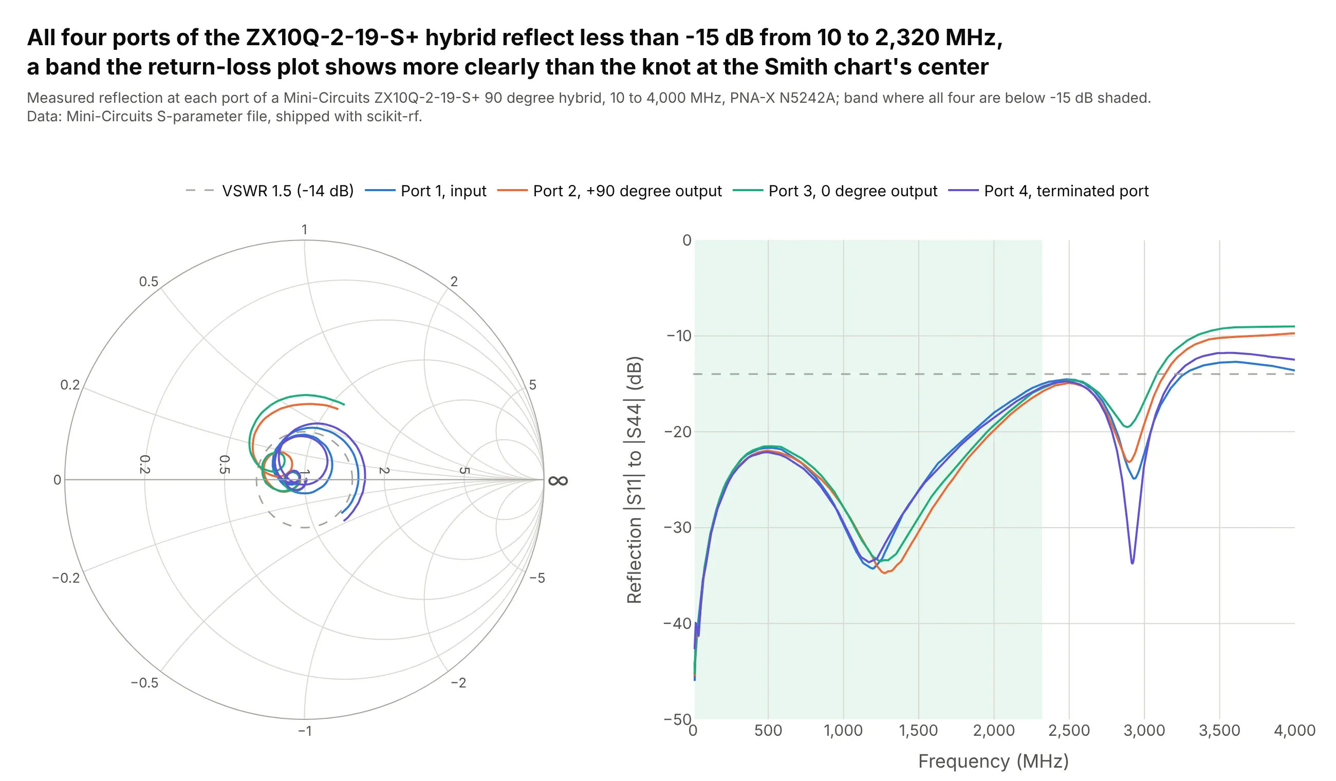
A Smith chart of the four port reflections of a Mini-Circuits ZX10Q-2-19-S+ hybrid, small loops around the center inside a dashed VSWR 1.5 circle, next to a line chart of the same four reflections in dB from 10 to 4,000 MHz with the band below -15 dB shaded up to 2,320 MHz

All four ports of the ZX10Q-2-19-S+ hybrid stay below -15 dB of reflection from 10 to 2,320 MHz. On the Smith chart that's a small knot around the center, so a return-loss plot beside it gives the band and the numbers. Data: Mini-Circuits S-parameter file, shipped with scikit-rf.

Tip: put a Smith chart and ordinary axes in one figure by giving layout.smith.domain and xaxis.domain different parts of the width.

Get the data from scikit-rf's documentation, the Mini-Circuits file
MiniCircuits_ZX10Q-2-19-S+___Plus25degC.s4p (a 90 degree hybrid measured on a PNA-X, 10 to 4,000 MHz), and
shape it into a table (columns: freq_mhz, param for S11, S22, S33, S44, gamma_re, gamma_im, mag_db).

Build a plotly figure with a Smith chart on the left and |S| in dB against frequency on the right, the same
color per port in both, a VSWR 1.5 circle and line, and the band where all four are below -15 dB shaded.

7. The same filter at two temperatures

Smith chart of the LFCN-2352+ filter's input reflection from 20 to 30 GHz at +25 C in blue and +125 C in red, two nearly parallel spirals, with each one's -3 dB point marked: 24.90 GHz at +25 C and 24.48 GHz at +125 C

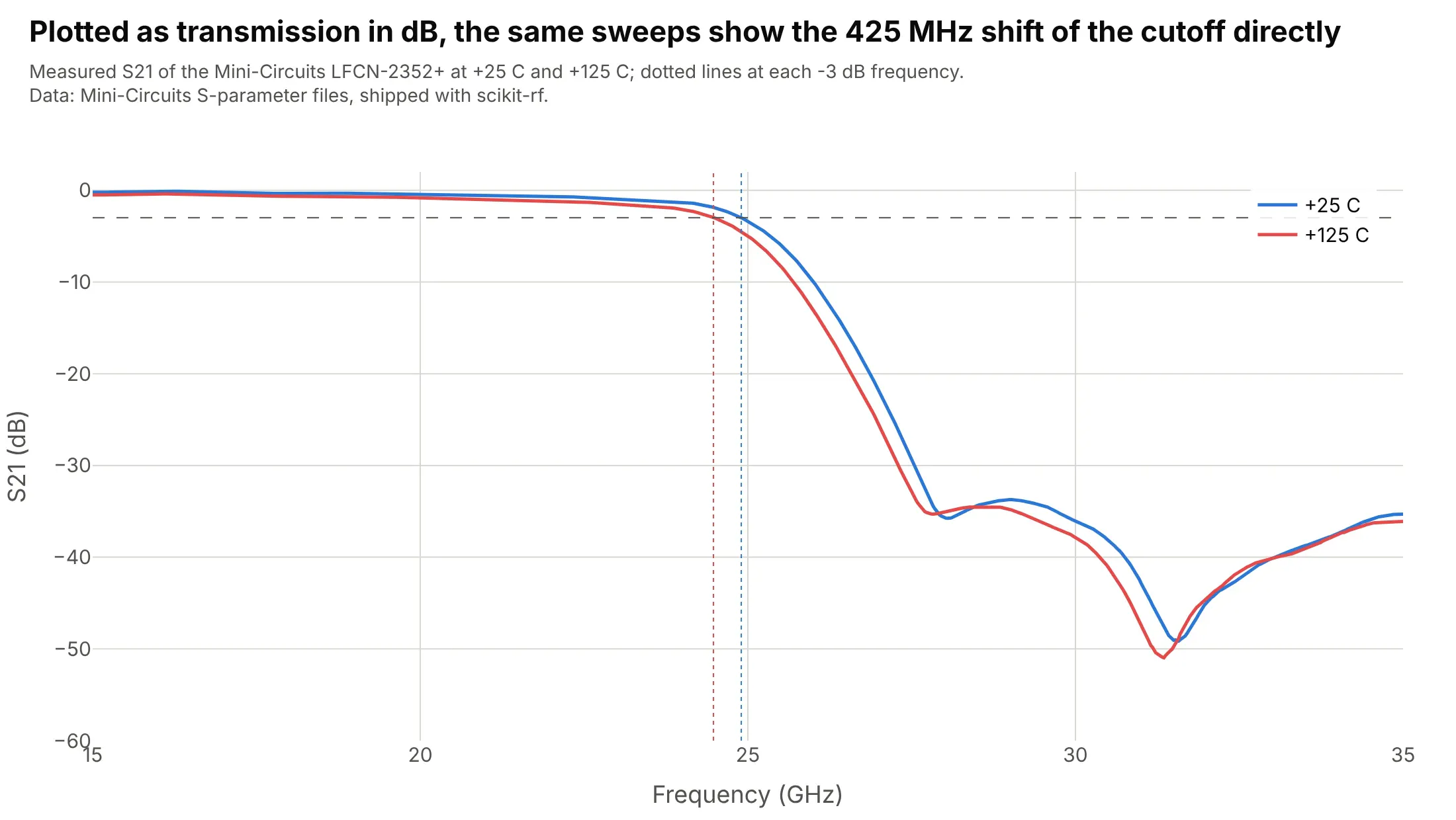
Heating the LFCN-2352+ filter from +25 C to +125 C moves its -3 dB edge 425 MHz lower, from 24.9 to 24.475 GHz, while its input impedance follows almost the same path. Data: Mini-Circuits S-parameter files at +25 C and +125 C, shipped with scikit-rf.

Tip: overlay two conditions on one Smith chart and mark the same event, here the -3 dB point, on both.

Get the data from scikit-rf's test data, the Mini-Circuits files LFCN-2352+_Plus25degC.s2p and
LFCN-2352+_Plus125degC.s2p (a low-pass filter measured at two temperatures), and shape them into a table
(columns: temperature, freq_mhz, param, gamma_re, gamma_im, mag_db).

Build a plotly Smith chart of S11 from 20 to 30 GHz at both temperatures, blue and red, with the frequency
where S21 falls through -3 dB marked on each curve.

Another way to see it: the cutoff itself is a transmission number, so S21 in dB against frequency shows the 425 MHz shift directly.

S21 in dB against frequency from 15 to 35 GHz at +25 C and +125 C, the red curve falling through -3 dB 425 MHz before the blue one