Carpet Plots - A Complete Guide

TL;DR

• A carpet plot shows how one result depends on two inputs by drawing a skewed grid: one family of lines for each value of the first input, another for each value of the second, and the result on the vertical axis. You read a value where two lines cross, and interpolate between them.
• Carpet plots are also known as cheater plots when the horizontal axis is a meaningless "cheater" axis, and as lattice plots when a third input adds more carpets. They are similar to contour plots, 3D surface plots and heatmaps, which show the same kind of data in other ways.
• Aerospace engineers use them for trade studies, most famously to size an aircraft from its wing loading (weight per wing area) and thrust-to-weight ratio, and they are standard for engine and compressor maps and for composite laminate stiffness.
• You can make a carpet plot with Plotly from a go.Carpet trace, then put points and lines on it with go.Scattercarpet and contours with go.Contourcarpet. The code is below.

What is a carpet plot?

Carpet plots look like this:

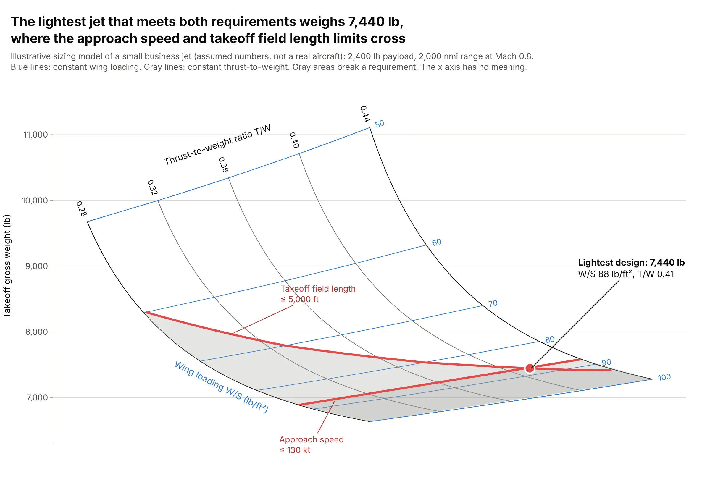
Data: computed from an illustrative sizing model of a small business jet with assumed numbers (2,400 lb payload, 2,000 nautical miles at Mach 0.8), not a real aircraft.

How do you read a carpet plot? In the example above, notice these things:

• Each crossing of a blue and a gray line is one candidate airplane. The blue lines hold the wing loading (W/S, takeoff weight divided by wing area, in lb per square foot) constant, the gray lines hold the thrust-to-weight ratio (T/W, engine thrust divided by weight) constant, and the height of the crossing is the takeoff gross weight that design ends up at.
• Moving down a gray line, toward a higher wing loading and so a smaller wing, the jet gets lighter: at T/W 0.36 it weighs 10,343 lb with a wing loading of 50 and 6,943 lb at 100. Moving along a blue line toward more thrust makes it heavier, because bigger engines weigh more.
• The horizontal axis has no meaning and is hidden. Each line of constant T/W is shifted sideways so the two families of lines cross at a readable angle; that shift is the "cheater" axis.
• The red lines are requirements: a takeoff field length of at most 5,000 ft needs more thrust as the wing gets smaller, and an approach speed of at most 130 knots caps the wing loading at 88. Everything in gray breaks one of them, so the lightest airplane that meets both, 7,440 lb, sits where the two lines cross.

It's often used for charts like these:

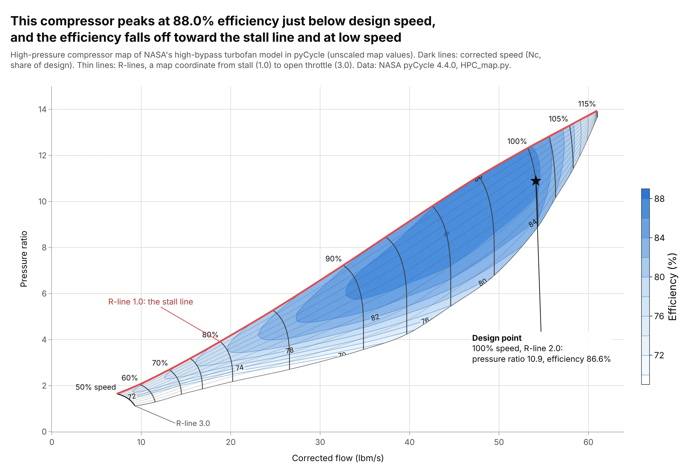
Engine and compressor maps. A compressor map is a true carpet with meaningful axes: lines of constant shaft speed cross lines of constant R-line (a map coordinate from the stall line to open throttle), and a contour carpet adds efficiency, which peaks at 88.0% in this map. Data: the high-pressure compressor map in pyCycle, the engine cycle code of the National Aeronautics and Space Administration (NASA), Apache 2.0 license.

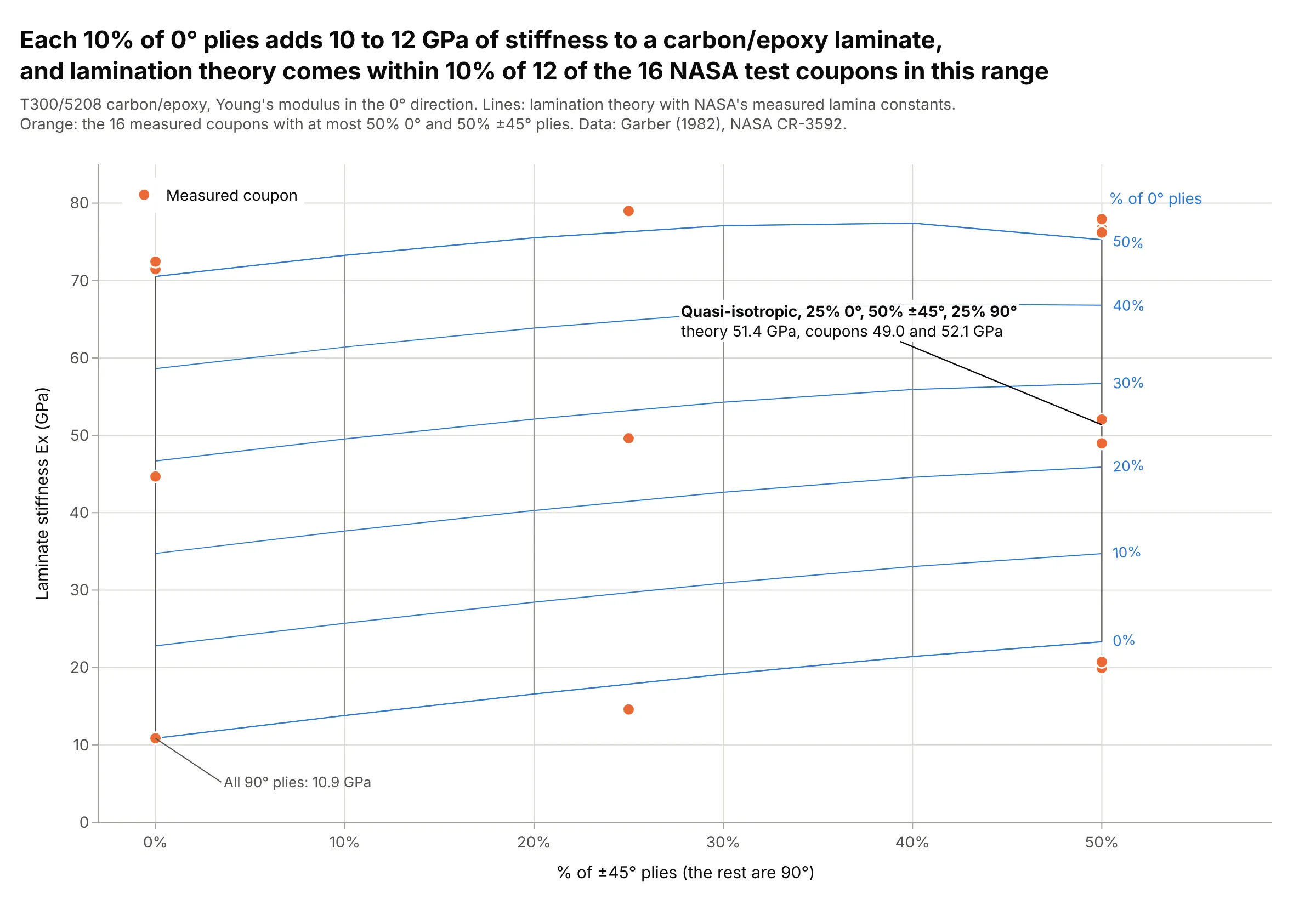
Composite laminates, the classic materials use. Designers of carbon fiber parts pick a ply mix from carpets like this one, where each 10% of 0° plies adds 10 to 12 GPa of stiffness, and lamination theory comes within 10% of 12 of the 16 NASA test coupons in range. Data: Garber (1982), NASA Contractor Report 3592, lamina constants and Table V.

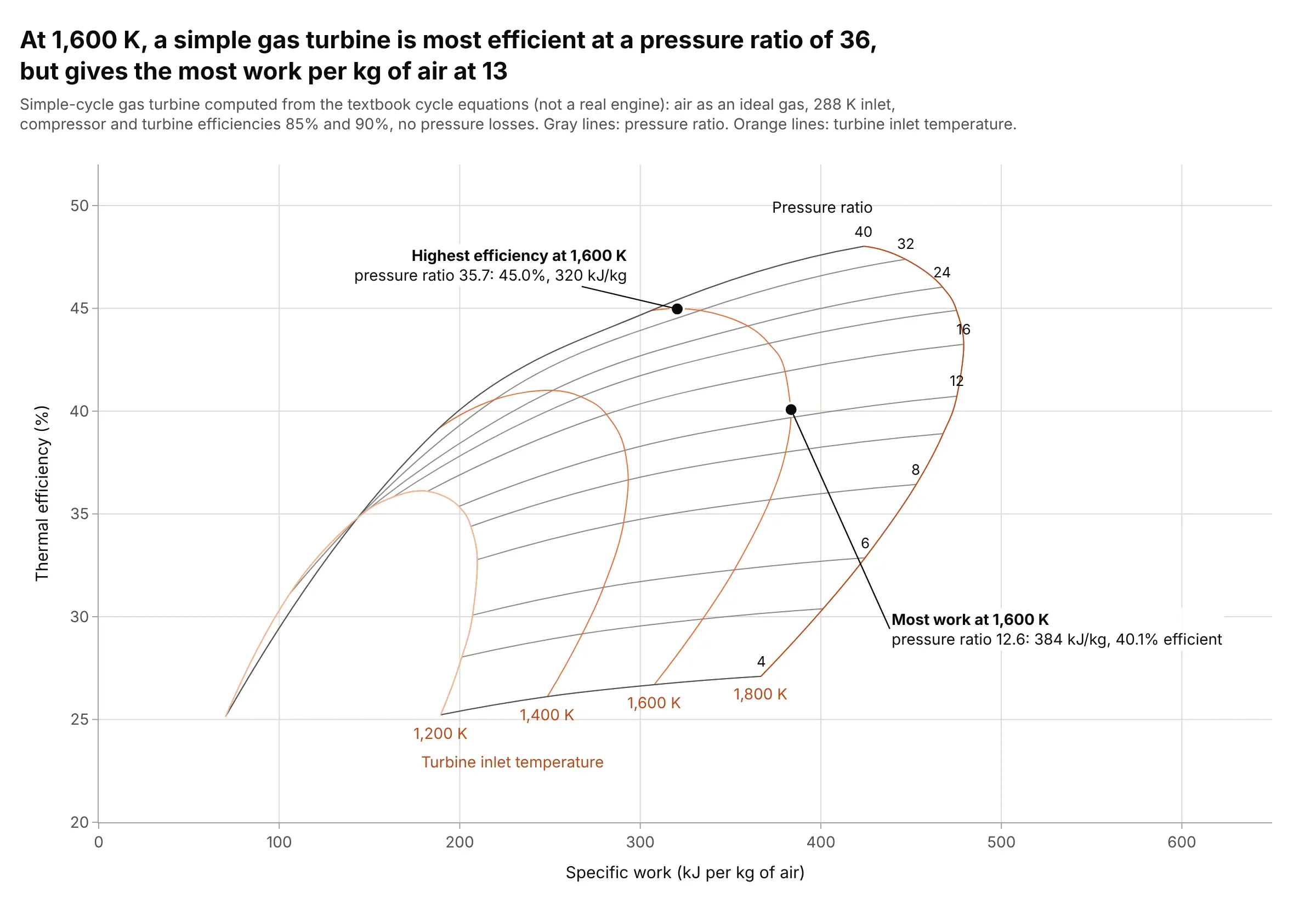
Engine cycle design, the textbook use. At a turbine inlet temperature of 1,600 K, this simple gas turbine is most efficient (45.0%) at a pressure ratio of 36 but delivers the most work per kilogram of air (384 kJ) at 13, a trade-off the carpet shows in one view. Data: computed from the textbook cycle equations with component efficiencies of 85% and 90%, not a real engine.

How to read a carpet plot

A carpet plot shows a function of two inputs, y = f(a, b), on a flat page. It is easier to read than it looks once you see how it is built from an ordinary line chart.

From a family of curves to a carpet

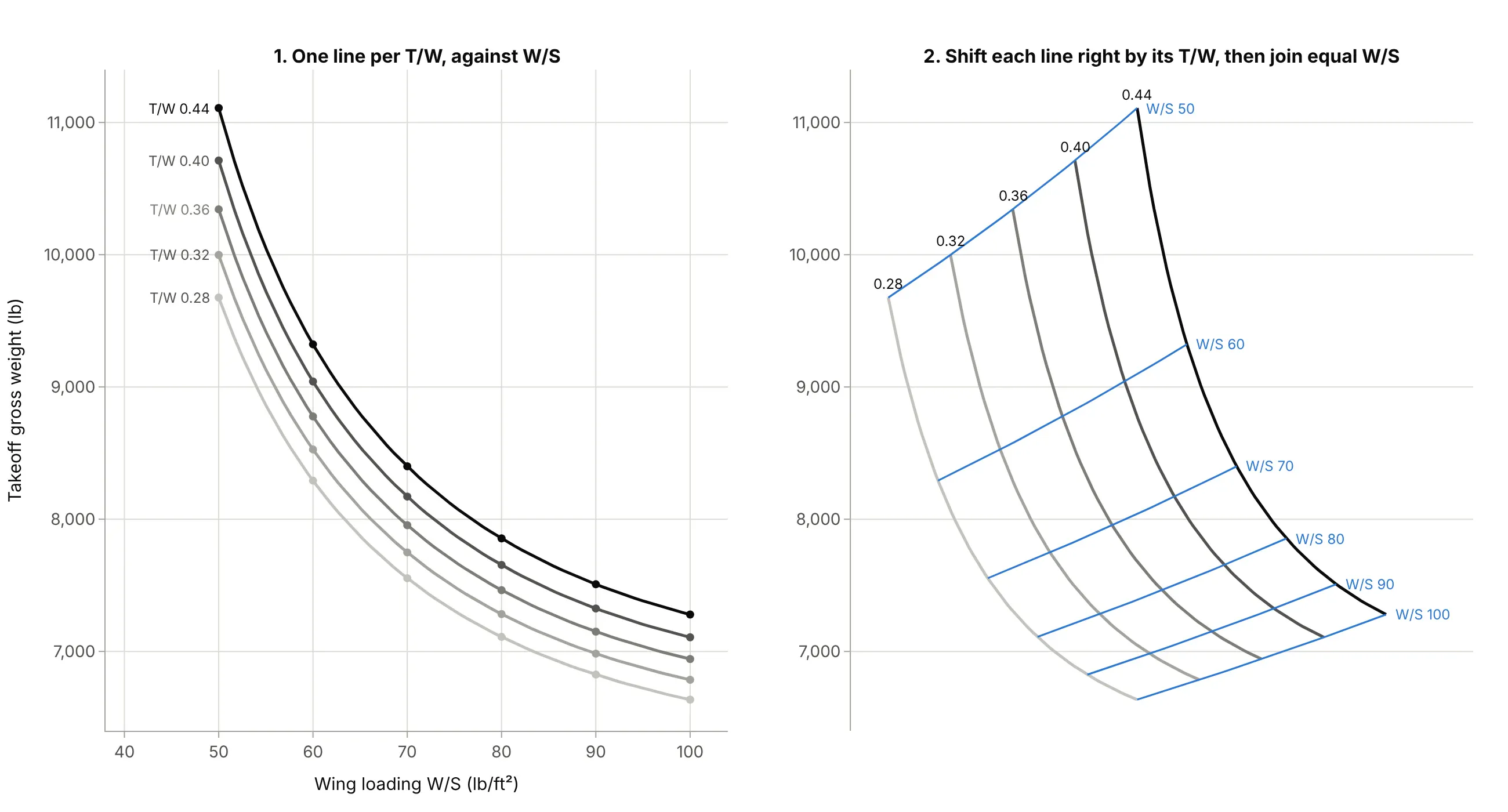
The usual way to draw y = f(a, b) is a family of curves: y against a, with one line for each value of b. When the lines are close together, as here, it is hard to tell which is which and harder to estimate a value between two lines. A carpet plot shifts each curve sideways by an amount proportional to its b value, then joins the points with equal a by a second set of lines:

Data: the illustrative sizing model from the main example (assumed numbers).

Nothing about y changes: every point is at the same height as before. The horizontal position is now a mix of a and b with no unit, which is why it is called a cheater axis and is usually hidden. What you gain is that both inputs are lines you can read, and every crossing is a grid point.

Reading a value between the lines

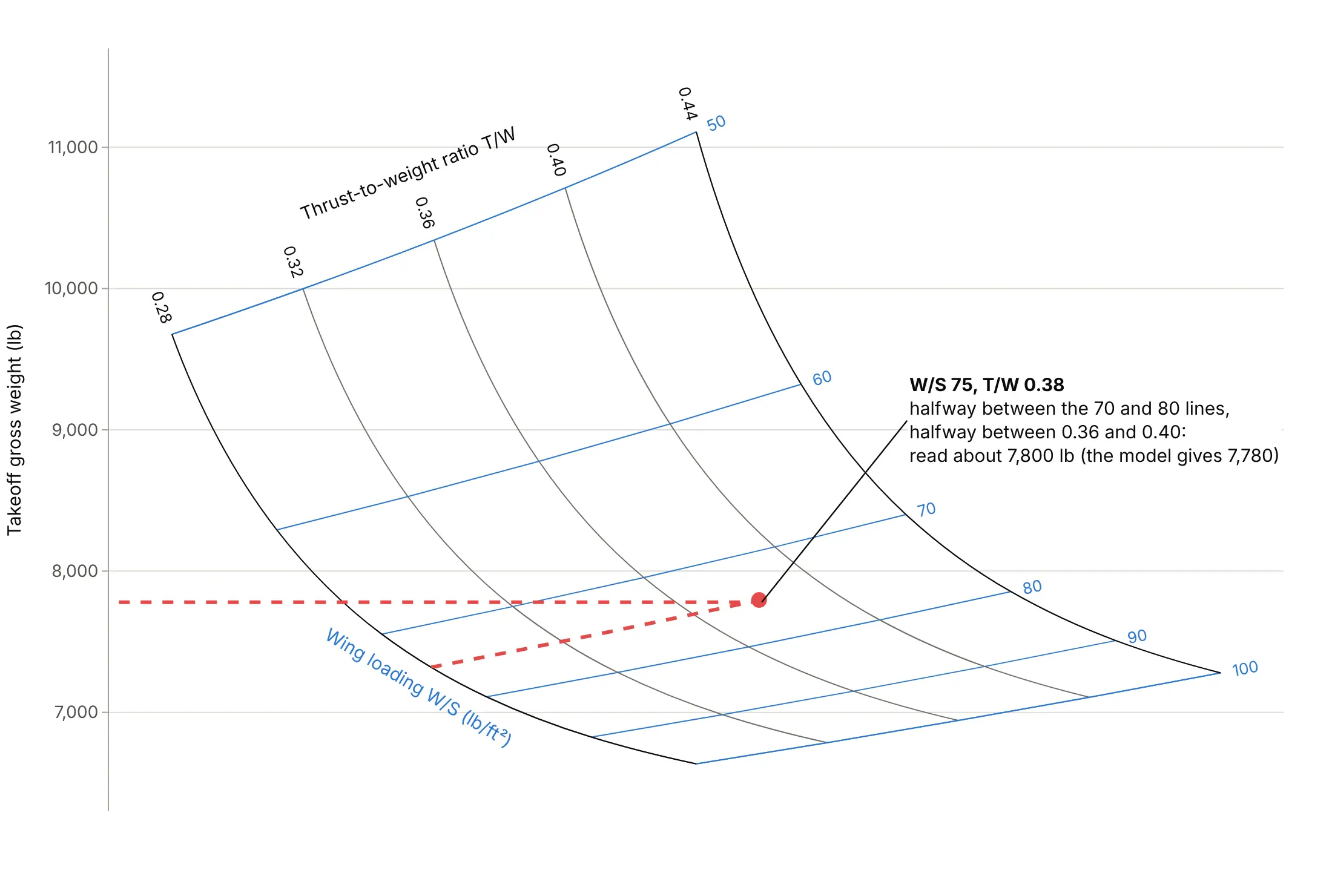
To read a design that is not on a line, find its place between the lines of each family and read the height straight across to the vertical axis:

Data: the illustrative sizing model from the main example (assumed numbers).

A wing loading of 75 and a T/W of 0.38 sit halfway between the 70 and 80 lines and halfway between 0.36 and 0.40, which reads as about 7,800 lb. The model gives 7,780 lb, and linear interpolation between the four corners of that cell gives 7,811 lb, so reading by eye loses less than 1%. More accurate interpolation is the main advantage of a carpet over a contour plot or a 3D surface, where a value between two contours or on a tilted surface has to be guessed.

Cheater plots and true carpet plots

When the result depends on two inputs and you have one output, the horizontal axis is a cheater axis and the carpet's skew is a choice: a steeper shift spreads the lines out, a gentler one makes the carpet narrower. When there are two outputs, such as efficiency and work for an engine, or pressure ratio and flow for a compressor, both axes mean something and the carpet's shape is fixed by the data. Wikipedia calls these a cheater plot (three variables) and a true carpet plot (four variables). True carpets can fold over themselves when two designs give the same pair of outputs, as the 1,200 K line does in the gas turbine example above.

Contour carpets and constraint lines

A third output can go on the same grid as contour lines (a "carpet with isolines"), like the compressor efficiency above, or the fuel weight in the examples below. Requirements that depend on the inputs, such as a field length or a speed limit, go on as lines in input coordinates, and the carpet bends them into place. In Plotly, go.Contourcarpet draws contours and go.Scattercarpet draws points and lines, both given in a and b, so you never convert them to x and y yourself.

A short history

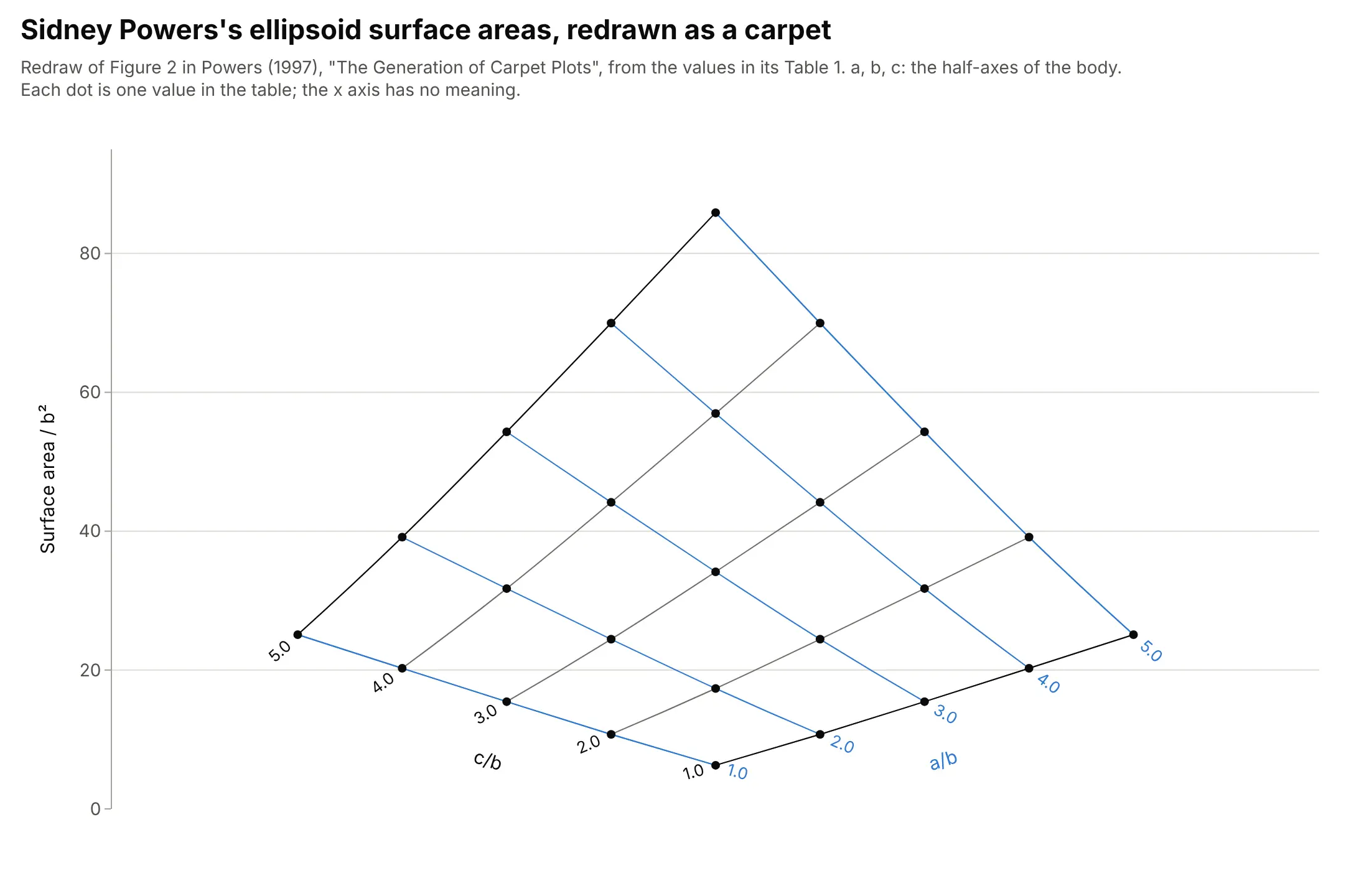
Carpet and lattice plots were in use in British aeronautics by the 1940s. R. Tatham's 1953 note in The Aeronautical Journal credits them to R. F. Sargent of the National Physical Laboratory and cites A. H. Yates, who described them with examples from aerodynamic and engine performance data in Aircraft Engineering in 1946; Tatham used them for structures data sheets and found interpolation easier and more accurate (Tatham 1953, as summarized on Cambridge Core). They became a standard tool of aircraft design for sizing trade studies, and a 1997 note by Sidney Powers on how to draw them, included in W. H. Mason's aircraft design course at Virginia Tech, uses the surface area of ellipsoids as its example, redrawn here:

Data: Table 1 of Sidney A. Powers, "The Generation of Carpet Plots" (1997), redrawn with Plotly.

Plotly added the carpet, scattercarpet and contourcarpet traces in plotly.js 1.26.0, released in April 2017.

Alternatives to a carpet plot

Here's the same sizing data drawn five ways. Some are better for the question, some worse, some just different:

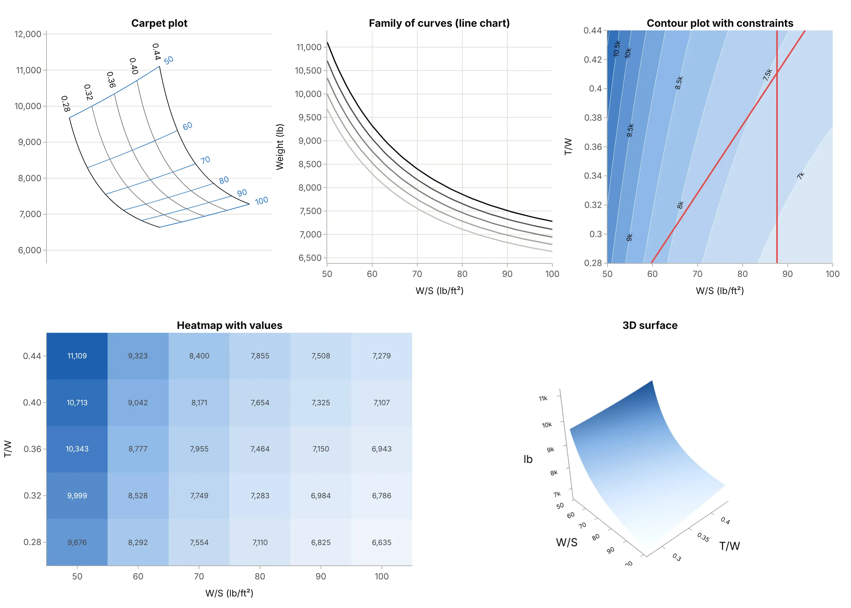
• Family of curves (works too, for a few lines). It's a line chart everyone can read, but the curves bunch together, and values between two curves are guesswork.
• Contour plot (better for finding the optimum). With the inputs on real axes, constraints become simple lines and the best feasible point is easy to see; this is the view aircraft designers call a thumbprint plot. Reading an exact weight means interpolating between contours. See our contour plot guide.
• Heatmap with values (better for exact numbers). A heatmap with the numbers printed is a table with color, precise at the grid points but with no way to interpolate or to draw constraints across it.
• 3D surface (worse on paper, different on screen). A 3D surface shows the shape well when you can rotate it, but no value can be read off a static view.
• Carpet plot (better for reading values for any pair of inputs). Both inputs are lines you can follow and interpolate between, and constraints and isolines fit on top, which is why trade studies use it.

For many cases at once, such as a carpet per Mach number, small multiples of carpets keep each one readable.

How to make a carpet plot

With AI

ChatGPT, Claude Code, GitHub Copilot, Cursor and other AI tools are excellent at writing Plotly code. Name Plotly in the prompt, and say which variable is a, which is b, and what goes on the axes:

With Plotly Studio

Plotly Studio is a desktop app where you point an AI at a dataset and it builds charts and a Dash app around your questions. Ask for a carpet plot the same way:

Show a carpet plot of pressure ratio against corrected flow from this compressor map, with one line per corrected speed and one per R-line, efficiency as labeled contours on the carpet, and the stall line in red.

Make a carpet plot in Python or JavaScript

This is the code AI tools write under the hood. A carpet takes the two inputs as a and b and the result as a 2D y with one row per b value. Leave out x and Plotly builds the cheater axis for you (its skew is set by cheaterslope); pass x as a second 2D array for a true carpet. This draws Powers's table from the history section and marks one point on it by its inputs:

To add contours, put a go.Contourcarpet(a=a, b=b, z=z, carpet="c") with the same carpet id before the carpet trace. In JavaScript, plotly.js uses the same three trace types:

Share it

Every Plotly chart has a Share chart button (the cloud icon in its toolbar) that uploads it to Plotly Cloud and gives you a link. Only you can see it until you change its visibility.

For a live app, put the chart in a Dash app and publish it with the Plotly Cloud CLI. Coding agents can run these commands for you:

If your data has to stay in your own cloud or data center, publish to Dash Enterprise instead.

Dos and don'ts

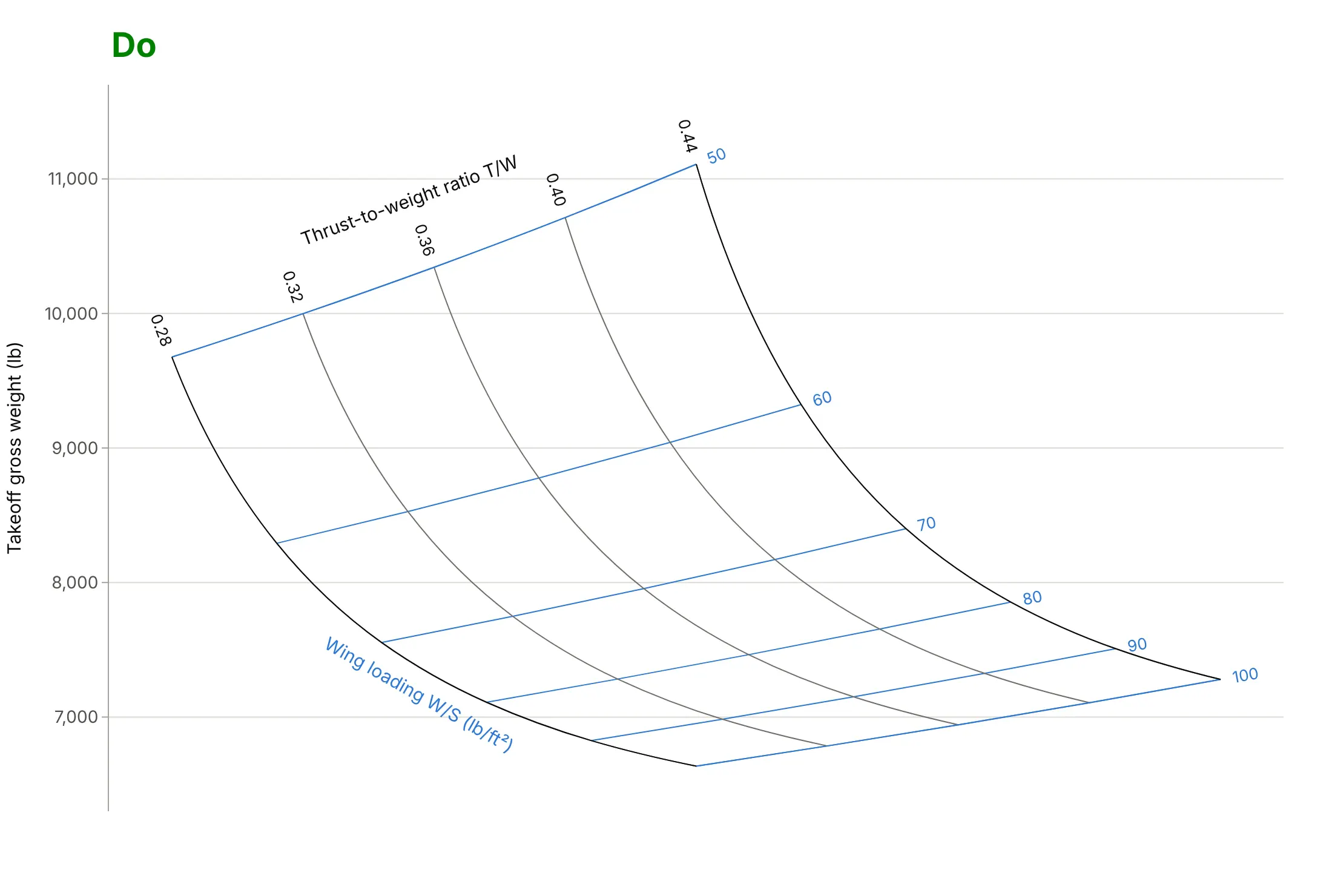
A carpet plot only works if readers can tell which line is which and know not to read the horizontal axis. Here is the sizing carpet both ways, with the same colors.

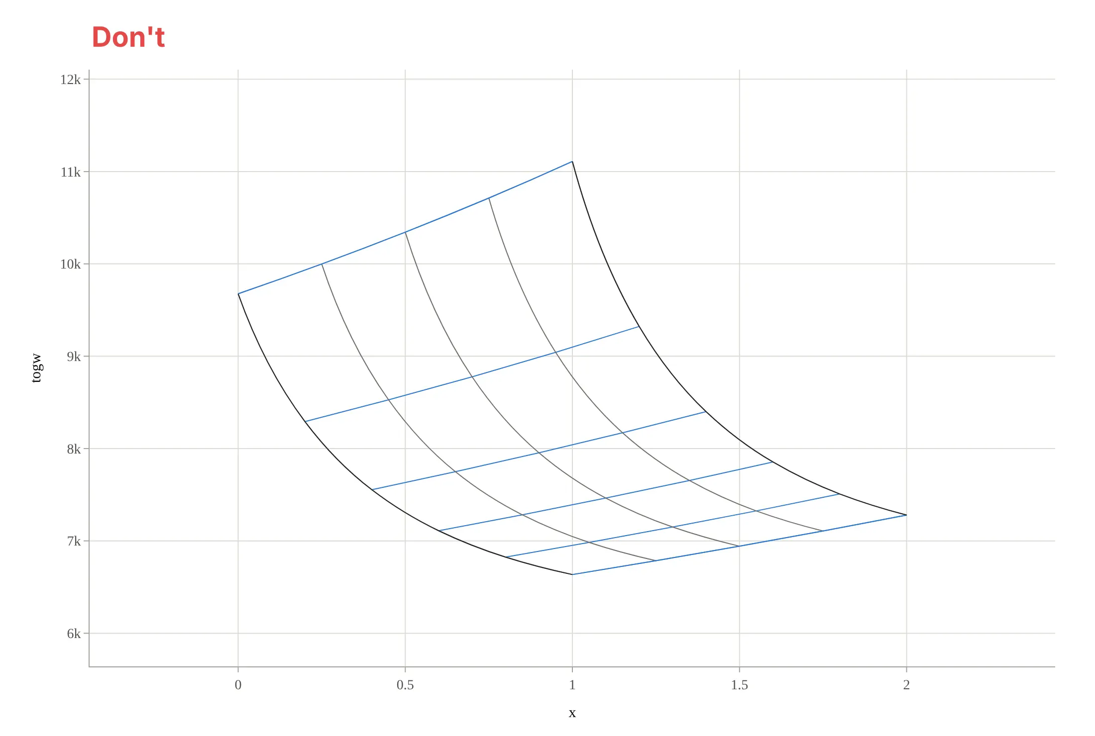
Don't show the cheater axis with numbers and a title (readers will try to read it), leave both families of lines unlabeled, use raw column names like "togw" and abbreviated numbers like "9k", and switch to a serif font:

Do hide the cheater axis, label every line with its value on the carpet's edges and name each family with its unit, and format the result axis with a name, a unit and full numbers:

Checklist

Do

• Label both families of lines, with values at the ends and the variable name and unit once.
• Hide the cheater axis, or say on the chart that it has no meaning.
• Use two distinct colors or weights for the two families, and keep constraint lines in a third, strong color.
• Choose a grid fine enough that straight-line interpolation between lines is close to the real value, and say on the chart which inputs are tabulated and which are interpolated.
• Say whether the data are measured, tabulated or computed from a model, and with which assumptions.

Don't

• Read a value off the horizontal axis of a cheater plot.
• Let smoothing (the smoothing option) bend a coarse grid into curves that overshoot the data; use smoothing=0 when the grid is coarse or the lines fold.
• Put more than about eight lines in each family on a printed carpet; label every other line instead.
• Use a carpet for data that are not on a full grid of the two inputs; fill the grid or use a scatter plot.

Options to customize

A carpet plot in Plotly is a go.Carpet trace, plus go.Scattercarpet and go.Contourcarpet traces that refer to it by its carpet id. These are the options that matter most; the full lists are in the carpet, scattercarpet and contourcarpet references and the carpet plot, carpet scatter and carpet contour tutorials.

1. a, b: the two inputs, as 1D lists (or 2D arrays the same shape as y). Each value becomes one line of the carpet.
2. y and x: the 2D results, one row per b value. Leave out x for a cheater plot; give it for a true carpet with a meaningful horizontal axis.
3. cheaterslope: how far each successive b line is shifted sideways in a cheater plot; change it, or its sign, to open up a carpet whose lines cross at a shallow angle.
4. carpet: an id that scattercarpet and contourcarpet traces use to find their carpet; needed when a figure has more than one carpet.
5. aaxis, baxis: the carpet's own axes: title, tickmode="array" with tickvals, tickformat, tickprefix, ticksuffix, and showticklabels ("start", "end", "both" or "none") for which edge carries the labels.
6. aaxis.gridcolor, gridwidth, startlinecolor, endlinecolor, minorgridcount: line colors and weights for each family, the carpet's edges, and extra unlabeled lines between the labeled ones.
7. aaxis.smoothing: 0 for straight segments between grid points, up to 1.3 for splines; 1 looks smooth but can overshoot a coarse grid.
8. go.Scattercarpet(a=..., b=..., carpet=...): markers, lines, text and filled regions placed by their input values, for constraints, design points and reading paths.
9. go.Contourcarpet(a=..., b=..., z=..., carpet=...) with contours.coloring ("fill", "lines" or "none") and contours.showlabels: isolines of a third quantity on the carpet.
10. layout.xaxis.visible=False: hides the cheater axis (Plotly hides it by default when x is left out).

More carpet plot examples

Six more carpet plots, each with its source, the technique that makes it work, and a prompt to rebuild it. Two use measured or published data, and four are computed from standard equations.

1. Density altitude: entering a cheater plot with two inputs

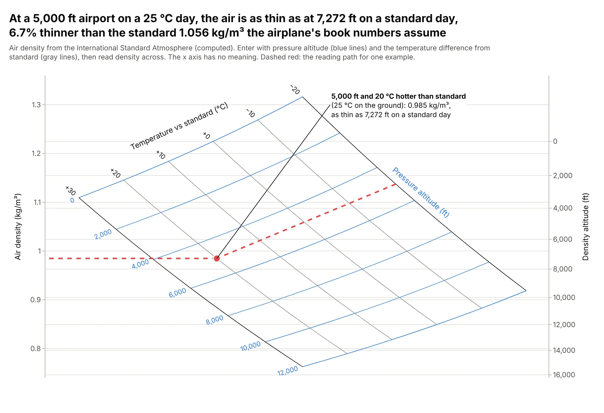
On a 25 °C day at a 5,000 ft airport, 20 °C warmer than standard, the air has a density of 0.985 kg/m³, the same as at 7,272 ft on a standard day and 6.7% less than the airplane's book numbers at 5,000 ft assume. Pilots call this the density altitude, and performance charts like this one are read exactly along the dashed path. Data: computed from the International Standard Atmosphere (ISA) equations.

Tip: draw the reading path in a strong color and add a second axis in the units people decide with, here density altitude in feet.

2. Fuel weight as isolines on the sizing carpet

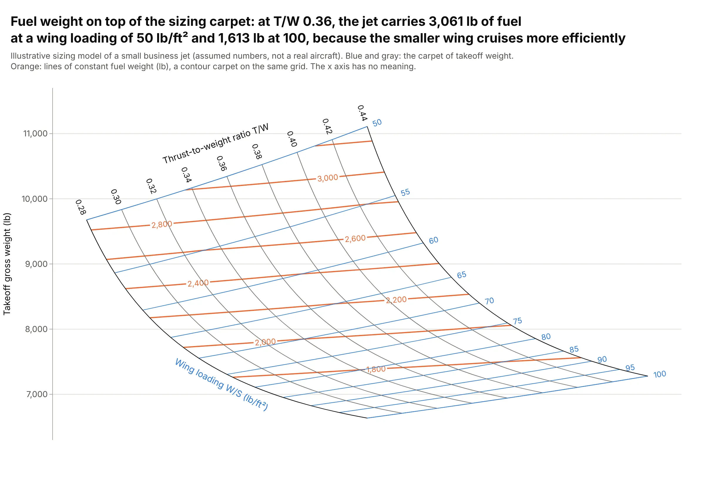
A contour carpet adds a third output to the sizing carpet: at a thrust-to-weight of 0.36, the jet carries 3,061 lb of fuel with a wing loading of 50 lb/ft² and 1,613 lb at 100, because the smaller wing flies closer to its best lift-to-drag ratio in cruise. The fuel lines cross the wing loading lines at a shallow angle: the wing sets most of the fuel, and a bigger engine adds some through the heavier airplane. Data: computed from the illustrative sizing model (assumed numbers).

Tip: set contours.coloring="none" so the isolines sit on the carpet without a fill that hides its lines.

3. Two carpets show the effect of a third input

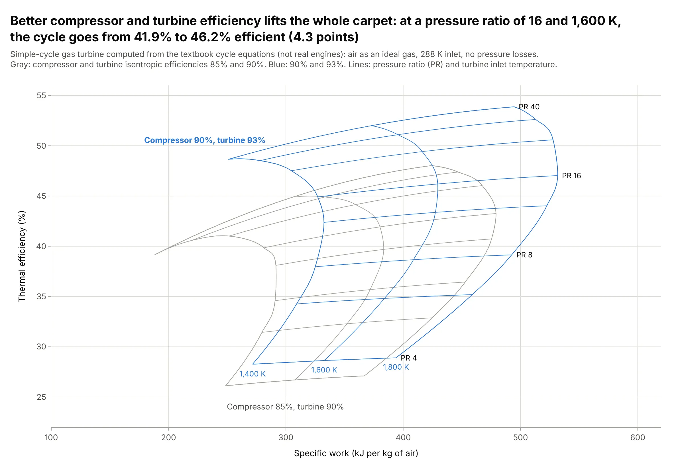
Raising the compressor's isentropic efficiency from 85% to 90% and the turbine's from 90% to 93% moves the whole carpet up and to the right: at a pressure ratio of 16 and 1,600 K, the cycle goes from 41.9% to 46.2% efficient and from 380 to 429 kJ of work per kilogram of air. Drawing a carpet per value of a third input is the idea behind lattice plots. Data: computed from the textbook cycle equations, not real engines.

Tip: draw the reference carpet in gray and label only the one you want readers to use.

4. Pressure around an airfoil on a curved mesh

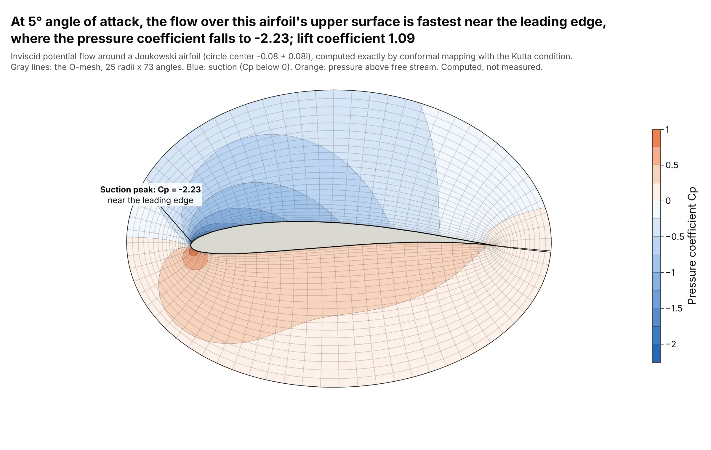
Computational fluid dynamics (CFD) results live on curved meshes that wrap around a body, and go.Carpet draws such a mesh from its two index directions, here distance from the surface and angle around it. On this airfoil at 5° angle of attack, the flow is fastest just behind the leading edge on the upper surface, where the pressure coefficient falls to -2.23, and the lift coefficient is 1.09. Data: computed exactly for inviscid flow with the Joukowski transform, not measured.

Tip: give the carpet the mesh's x and y and contour the solution with go.Contourcarpet; no regridding is needed.

5. Stocks, bonds and bills since 1928

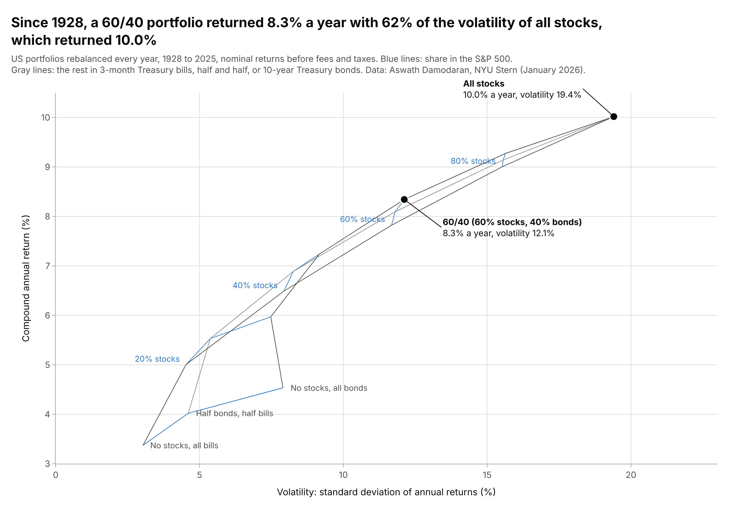
From 1928 to 2025, a portfolio of 60% S&P 500 stocks and 40% 10-year Treasury bonds, rebalanced every year, returned 8.3% a year with 62% of the volatility of all stocks, which returned 10.0%. The carpet folds near 40% stocks, where a mix of stocks and bonds and a mix with more stocks and bills give about the same risk and return. Data: Aswath Damodaran, NYU Stern, annual returns 1928 to 2025.

Tip: use smoothing=0 on a true carpet that folds, so the lines go straight between the computed portfolios.

6. Drug dosing regimens against an exposure target

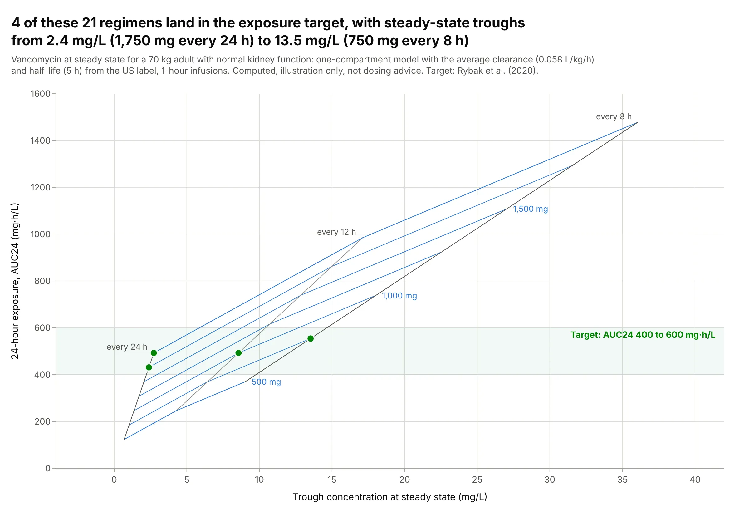
For a 70 kg adult with average kidney function, four of these 21 regimens put the 24-hour exposure (the area under the concentration curve, AUC24) in the 400 to 600 mg·h/L target, with steady-state troughs from 2.4 mg/L (1,750 mg every 24 hours) to 13.5 mg/L (750 mg every 8 hours). The same exposure can come with very different troughs, which is why pharmacists look at both. Data: computed with a one-compartment model from the average clearance and half-life in the Pfizer vancomycin label, target from Rybak et al. (2020); an illustration, not dosing advice.

Tip: shade the target range as a band behind the carpet and mark the grid points inside it.