
Chris Parmer
November 15, 2026
Phase Diagrams - A Complete Guide
TL;DR
- A phase diagram is a map of which phase (solid, liquid, gas or a mix) a material is in at each temperature and pressure, or, for an alloy or a mixture, at each temperature and composition. Its lines mark where two phases coexist at equilibrium, its triple point is where three do, and the boiling line ends at the critical point, beyond which liquid and gas are no longer different.
- Phase diagrams are also known as equilibrium diagrams, and a one-substance diagram is called a pressure-temperature (P-T) diagram. A two-component version, drawn as temperature against composition, is a binary phase diagram, and a three-component one is a ternary plot. Pressure is usually on a logarithmic axis, because the boundaries span many orders of magnitude.
- Chemists, materials scientists and chemical engineers read them to choose process conditions. Examples include supercritical carbon dioxide (CO2) for coffee decaffeination and carbon capture pipelines, freeze-drying of biologics, liquefied natural gas (LNG), refrigerants, steel heat treatment, solder alloys and distillation.
- You can make a phase diagram with Plotly from go.Scatter lines computed from reference equations or a thermodynamic database, with filled polygons for the regions and markers for the triple and critical points. The code is below.
What is a phase diagram?
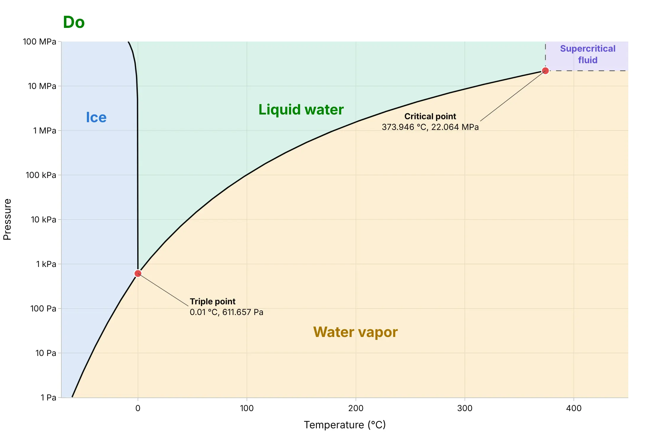
Phase diagrams look like this:
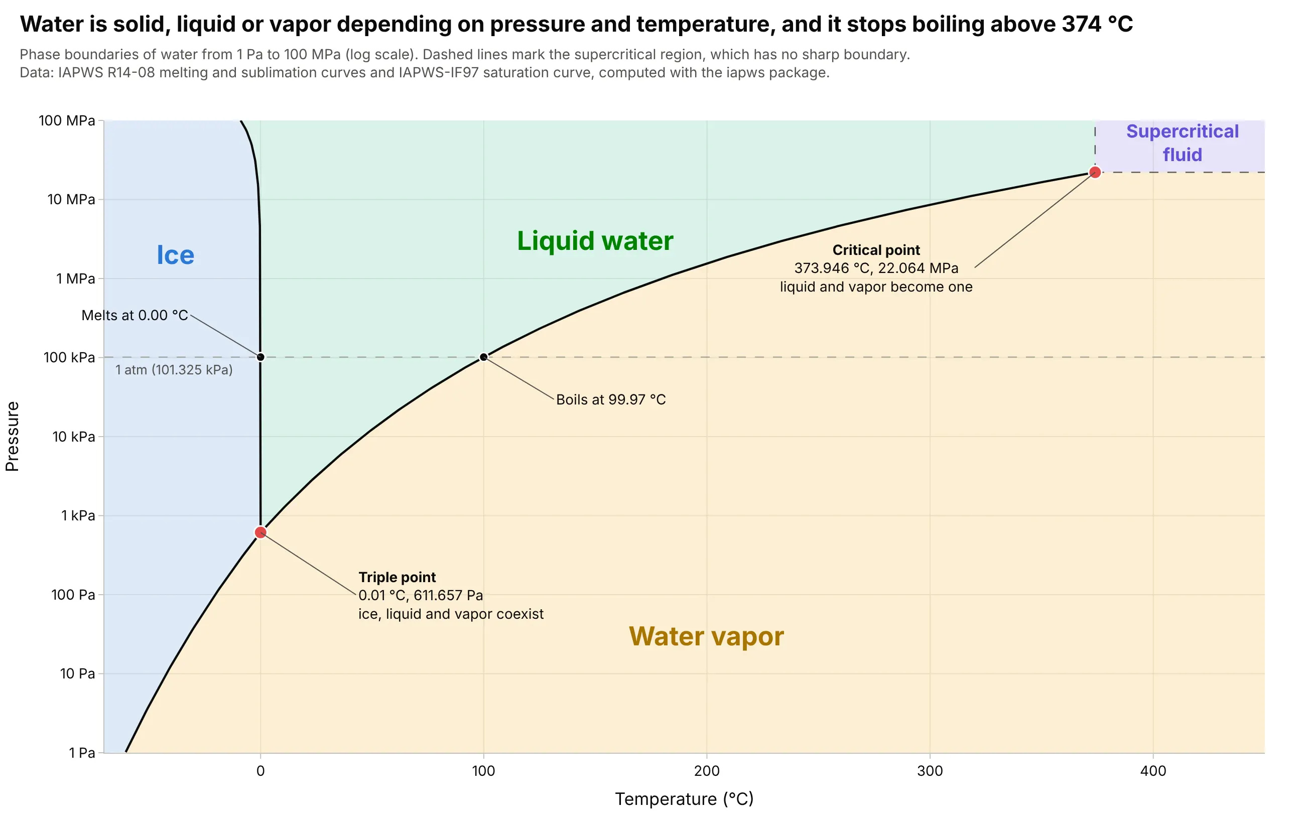
Data: boundaries computed with the iapws Python package, which implements the reference equations of the International Association for the Properties of Water and Steam (IAPWS): the melting and sublimation curves and the IAPWS-IF97 saturation curve.
How do you read a phase diagram? In the example above, notice these things:
- Each tinted area is one phase of water, and the black lines are where two phases are in equilibrium and can exist side by side. At 1 atm (a standard atmosphere, 101.325 kPa), walking across the diagram from left to right crosses the melting line at 0.00 degrees C and the boiling line at 99.97 degrees C, which is the familiar freezing and boiling of water.
- The melting line leans to the left, which is unusual, because ice is less dense than liquid water and so melts at a lower temperature when it is squeezed: -0.7 degrees C at 10 MPa and -8.9 degrees C at 100 MPa. The carbon dioxide chart below leans to the right, as it does for most substances.
- The triple point at 0.01 degrees C and 611.657 Pa (0.006 atm) is the single temperature and pressure where ice, liquid water and vapor coexist. Below that pressure liquid water cannot exist at any temperature, so ice turns straight into vapor, which is how freeze-drying works.
- The boiling line stops at the critical point, 373.946 degrees C and 22.064 MPa. Above both values liquid and vapor merge into one supercritical fluid, and the dashed lines that bound it are a convention and not a phase change. The pressure axis is logarithmic, so each gridline is ten times the one below, which is the only way to fit 611.657 Pa and 22.064 MPa on one chart.
It's often used for charts like these:
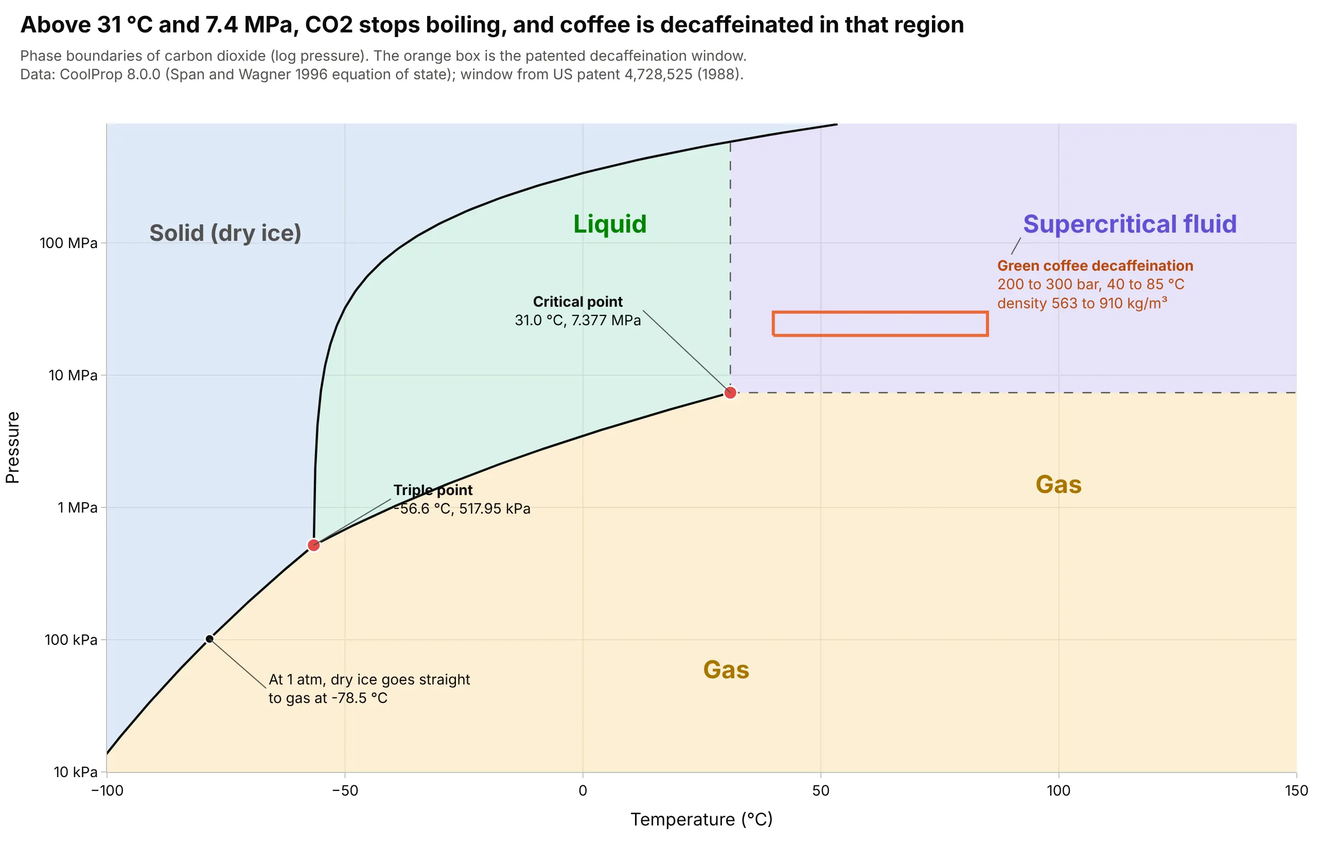
Supercritical carbon dioxide extraction. Carbon dioxide's triple point pressure is 517.95 kPa, 5.1 times atmospheric pressure, so dry ice cannot melt in open air and sublimes at -78.5 degrees C instead. A coffee decaffeination patent (US 4,728,525) works in the supercritical region at 200 to 300 bar and 40 to 85 degrees C, where the CO2 has the density of a liquid, 563 to 910 kg/m³. Data: CoolProp 8.0.0 with the Span and Wagner (1996) equation of state; the process window is from US patent 4,728,525 (Toro and Quijano, 1988).
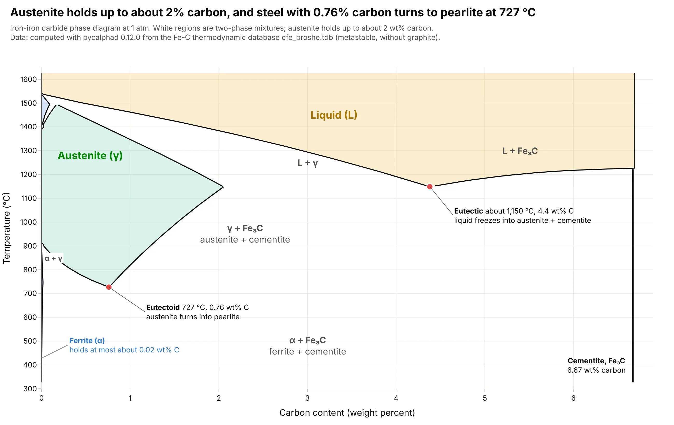
The iron-carbon diagram, the classic of metallurgy. Every carbon steel is read off this chart, which shows that steel with 0.76 weight percent (wt%) carbon turns from austenite into pearlite at 727 degrees C, and that austenite can dissolve about 2 wt% carbon at most (2.03 wt% at 1,146 degrees C according to Wikipedia, 2.05 wt% in the computed diagram). Data: computed with pycalphad 0.12.0 from an iron-carbon thermodynamic database file (cfe_broshe.tdb, the metastable iron-cementite system, which ships with pycalphad's tests).
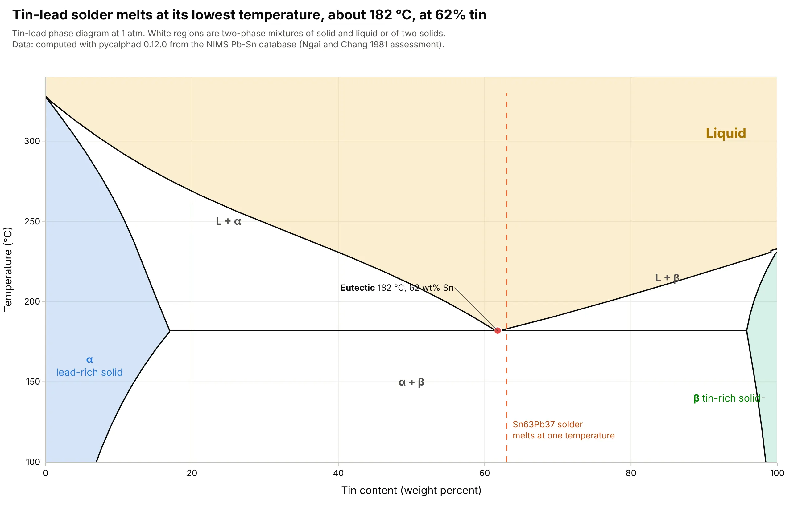
Solder alloys, the textbook eutectic. In a binary diagram a eutectic is the one composition that melts at a single temperature, the lowest in the system, and the computed tin-lead eutectic is 182 degrees C at 62 wt% tin. Wikipedia gives 183 degrees C for the 63 wt% tin solder (Sn63Pb37), and the European Union's Restriction of Hazardous Substances (RoHS) directive, in force since July 1, 2006, pushed electronics toward lead-free tin-silver-copper alloys, whose ternary eutectic is 217 degrees C and which are drawn on a ternary plot. Data: computed with pycalphad 0.12.0 from the Japanese National Institute for Materials Science (NIMS) tin-lead database (pbsn.tdb, from the Ngai and Chang 1981 assessment).
How to read a phase diagram
A phase is a region of a material that is uniform in composition and structure, such as ice, liquid water or water vapor. Different crystal structures of one solid count as different phases, which is why iron has ferrite and austenite. A phase diagram records which phases are stable at equilibrium, meaning after the material has had enough time to settle, so it describes where a material is heading and not always where a fast process leaves it.
Lines, areas and points: the phase rule
Josiah Willard Gibbs published the phase rule in his paper "On the Equilibrium of Heterogeneous Substances" (1875 to 1878). It says that the number of things you can change freely (the degrees of freedom, F) equals the number of components (C) minus the number of phases present (P) plus 2, or F = C - P + 2. For water, C = 1, so inside a single-phase area F = 2, and you can change temperature and pressure independently. On a line two phases coexist, F = 1, and fixing the temperature fixes the pressure, which is why water at 100 degrees C boils at exactly one pressure. At the triple point three phases coexist and F = 0, so nothing can change. A binary phase diagram is usually drawn at constant pressure, which removes one degree of freedom (F = C - P + 1), so a eutectic, where a liquid and two solids coexist, is also a point with F = 0.
The supercritical region and the logarithmic axis
Along the boiling line, the liquid and the vapor above it become more alike as temperature and pressure rise, until at the critical point they have the same density and the line ends. Past it there is a single supercritical fluid whose density can be tuned from gas-like to liquid-like by changing the pressure, which is what makes it useful as a solvent. The lines on a pressure-temperature diagram change by factors of millions, from 611.657 Pa at water's triple point to 22.064 MPa at its critical point, so pressure is drawn on a log axis, and the tick labels are better written with units (kPa, MPa) than as powers of ten.
Composition axes, liquidus and solidus
A binary diagram puts composition on the x axis, as weight percent (wt%) or as a mole fraction, and temperature on the y axis, at one pressure. The liquidus is the line above which the mixture is entirely liquid and the solidus is the line below which it is entirely solid, and between them liquid and solid coexist as a slushy mix. A solvus is the equivalent line between two solid regions. The point where the liquidus lines of two components meet at the lowest melting temperature is the eutectic, and the equivalent point where one solid turns into two other solids on cooling is a eutectoid. For a mixture of liquids, such as ethanol and water, the same two lines are called the bubble point (where the first vapor appears) and the dew point (where the last liquid disappears).
The tie line and the lever rule
To find out what a mixture contains at a given temperature, draw a horizontal tie line through its composition and temperature, from one boundary of the two-phase region to the other. The ends of the tie line give the compositions of the two phases. The lever rule gives how much of each there is, by treating the tie line as a lever balanced on the alloy's composition. The share of one phase is the length of the lever arm on the far side divided by the whole line, so the phase whose composition lies nearer the alloy is the larger one.
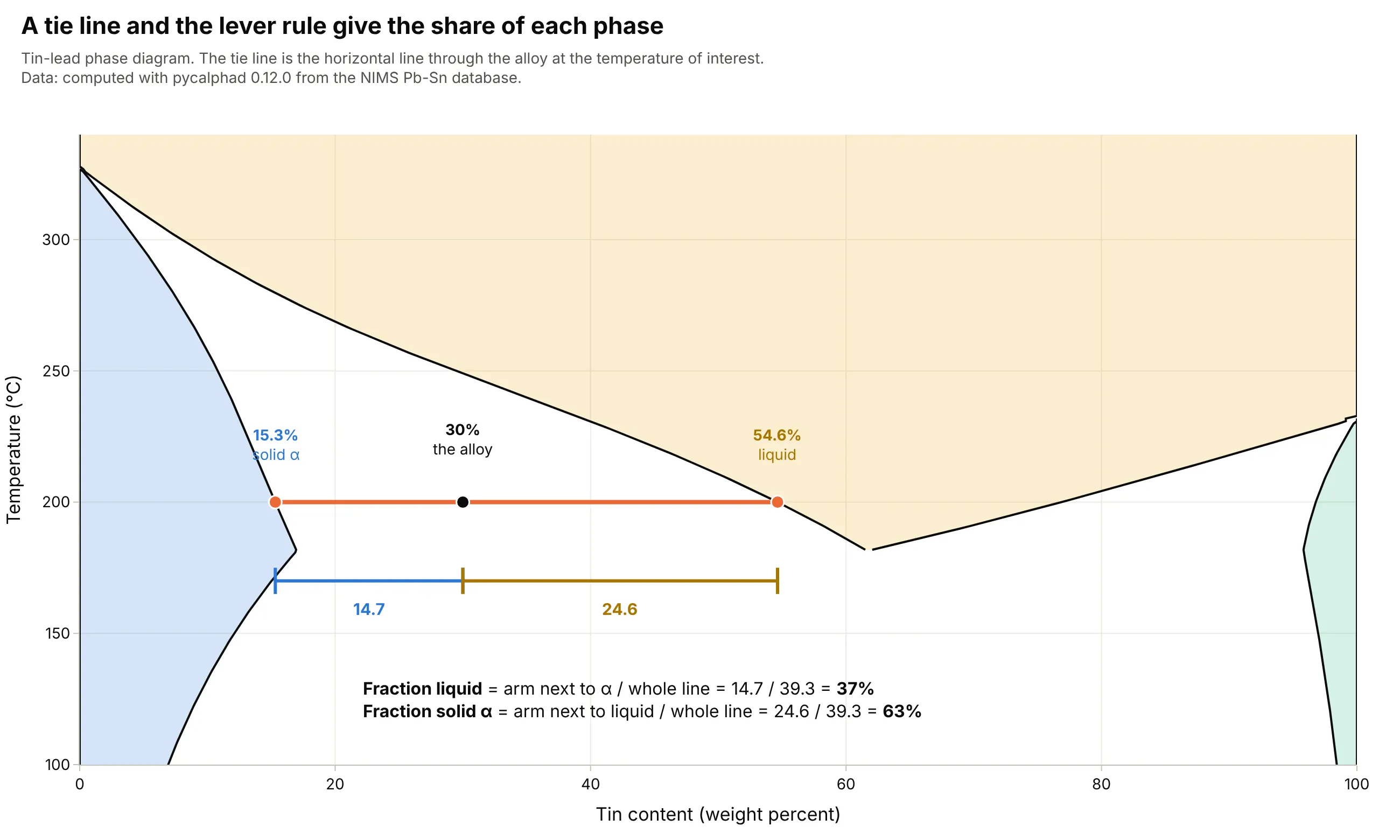
Data: computed with pycalphad 0.12.0 from the NIMS tin-lead database. At 200 degrees C a 30 wt% tin alloy lies 14.7 wt% from the solid and 24.6 wt% from the liquid, so it is 14.7 / 39.3 = 37% liquid and 63% solid.
The iron-carbon diagram in a few lines
Iron and carbon form a few phases that appear throughout steel. Ferrite is iron with almost no carbon (at most about 0.02 wt%, per Wikipedia), austenite is the high-temperature form of iron that dissolves up to about 2 wt% carbon, and cementite (Fe3C) is the hard compound iron carbide, at 6.67 wt% carbon. When austenite with 0.76 wt% carbon cools below 727 degrees C it turns into pearlite, a layered mix of ferrite and cementite, which is the eutectoid reaction. Carbon steels are usually taken to have less than about 2 wt% carbon, close to the austenite limit, and Wikipedia gives 0.76 wt% carbon and 727 degrees C for the eutectoid.
Where the lines come from
For a pure substance, the lines are the solutions of an equation of state, a fitted formula that gives pressure, density and energy for every temperature, and reference-quality ones exist for water, carbon dioxide and more than a hundred other fluids. For alloys they come from CALPHAD (CALculation of PHAse Diagrams), a method that stores a fitted Gibbs energy (the energy that every phase tries to minimize) for each phase in a thermodynamic database file, and finds the stable phases at every temperature and composition by minimizing the total. This guide uses iapws for water, CoolProp for carbon dioxide and other fluids, pycalphad for the alloys, and the thermo package's activity models for mixtures of liquids.
A short history
In 1869 Thomas Andrews showed that carbon dioxide cannot be liquefied by pressure alone above about 31 degrees C, a limit he named the critical point, and Wikipedia quotes his estimate of 30.92 degrees C against a modern value of 30.98. His Bakerian Lecture (published in Philosophical Transactions of the Royal Society, volume 159) plotted pressure against volume at several temperatures, and the picture below shows the same kind of figure redrawn with today's equation of state:
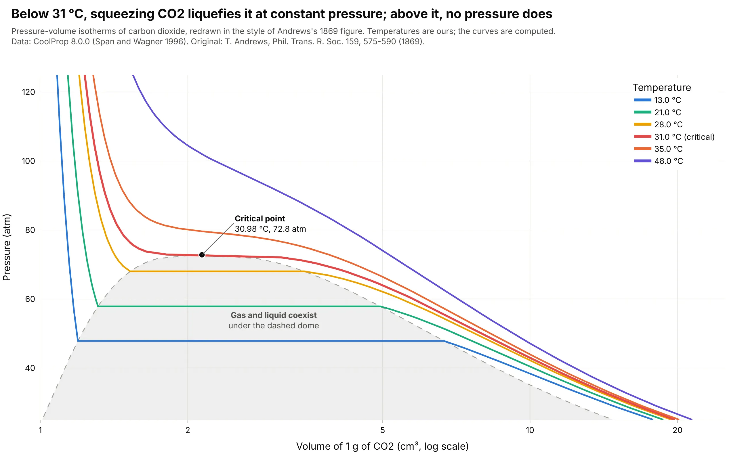
Data: computed with CoolProp 8.0.0 (Span and Wagner 1996). The temperatures are ours, not Andrews's, and the curves are computed and are not his measurements.
Gibbs's phase rule followed in 1875 to 1878, and the binary and iron-carbon diagrams of the late 1800s and early 1900s became the working tools of metallurgists. Today most of them are computed from thermodynamic databases and not drawn from experiments by hand.
Alternatives to a phase diagram
Here's the same carbon dioxide drawn six ways. Some are better for the question, some worse, some just different:
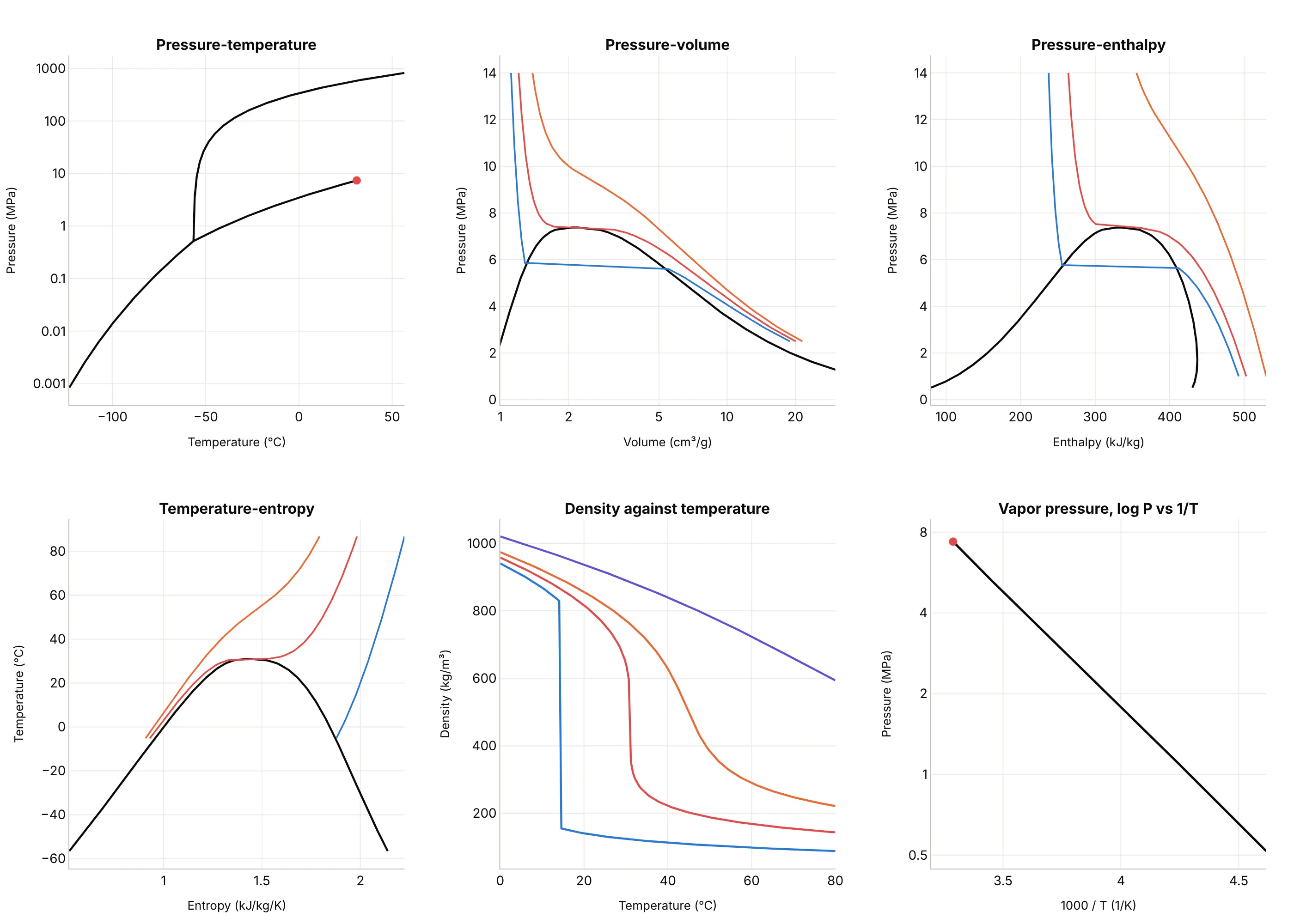
- Pressure-temperature phase diagram (the best map of phases). It answers which phase a material is in and where the boundaries and the critical and triple points are, but it hides how much volume, energy or entropy changes along the way.
- Pressure-volume isotherms (works too). The Andrews picture shows the coexistence dome and how the flat section shrinks to a point at the critical isotherm, which is useful for equations of state, though it has no solid phase.
- Pressure-enthalpy diagram (better for refrigeration). Refrigeration engineers use it because the heat added or removed in a compressor, condenser or evaporator is a horizontal distance on it.
- Temperature-entropy diagram (better for power cycles). Turbine and steam-cycle engineers use it because the work and heat of a cycle are areas on it.
- Density against temperature (different). A line chart shows a supercritical fluid's density tuning smoothly with temperature while the 5 MPa line drops at once at its boiling point, but it carries no phase boundaries.
- Vapor pressure on a log axis against 1/T (better for extrapolating). The saturation line is nearly straight, so a regression line fits it and gives the vapor pressure outside the measured range, which is how the Antoine equation (a three-parameter vapor pressure fit) works, but it has no other phases.
When the density or another property is the thing to see across the whole plane, a heatmap or contour plot under the phase boundaries works well, as in the carbon capture example below. For moist air, the same idea of a physics grid behind the data is the psychrometric chart.
How to make a phase diagram
With AI
ChatGPT, Claude Code, GitHub Copilot, Cursor and other AI tools are excellent at writing Plotly code. Name Plotly in the prompt, and ask for the boundaries to come from a reference library so the physics is right:
Make a plotly phase diagram of water: temperature in degrees C on x and pressure on a log y axis from 1 Pa to 100 MPa.- Compute the boundaries with the iapws package: the boiling line with iapws.iapws97._PSat_T, and the sublimationand melting lines of ice Ih with iapws._iapws._Sublimation_Pressure and _Melting_Pressure.- Fill the regions (ice, liquid, vapor, supercritical fluid) with light tints and draw the boundaries as heavy lines.- Mark the triple point (273.16 K, 611.657 Pa) and the critical point (647.096 K, 22.064 MPa) with labeled markers.- Label the pressure ticks with units (Pa, kPa, MPa), and draw the supercritical boundaries as thin dashed lines.- Check: at 1 atm (101325 Pa) water should boil at 99.97 C.
With Plotly Studio
Plotly Studio is a product for creating data visualizations and Dash apps and for analyzing data with AI, available as a desktop app or embedded in Dash apps. Ask for a phase diagram the same way:
Draw the pressure-temperature phase diagram of this fluid on a log pressure axis, with the saturation line computed from CoolProp, the triple and critical points labeled, and a dropdown to switch between fluids.
Make a phase diagram in Python or JavaScript
This is the code AI tools write under the hood. You can make a phase diagram with Plotly from go.Scatter lines computed from reference equations, with a log y axis. This function returns a go.Figure of the water diagram, and the examples in this guide add filled regions and annotations to the same idea:
import numpy as npimport plotly.graph_objects as gofrom iapws import _iapws, iapws97 # the iapws package implements the IAPWS reference equationsT_TRIPLE, T_CRIT = 273.16, 647.096 # kelvindef water_phase_diagram():"""Water's pressure-temperature phase diagram from the IAPWS reference equations, as a go.Figure."""t_boil = np.linspace(T_TRIPLE, T_CRIT, 300)t_sub = np.linspace(210, T_TRIPLE, 200)t_melt = np.linspace(251.165, T_TRIPLE, 200)curves = {"Boiling (liquid and vapor)": (t_boil, [iapws97._PSat_T(t) * 1e6 for t in t_boil]), # IAPWS-IF97"Sublimation (ice and vapor)": (t_sub, [_iapws._Sublimation_Pressure(t) * 1e6 for t in t_sub]), # IAPWS R14"Melting (ice and liquid)": (t_melt, [_iapws._Melting_Pressure(t) * 1e6 for t in t_melt]), # IAPWS R14}fig = go.Figure()for name, (t, p) in curves.items():fig.add_trace(go.Scatter(x=np.array(t) - 273.15, y=p, mode="lines", name=name, line=dict(width=3)))for name, t, p in (("Triple point", T_TRIPLE, 611.657), ("Critical point", T_CRIT, 22.064e6)):fig.add_trace(go.Scatter(x=[t - 273.15], y=[p], mode="markers+text", text=[name], textposition="top left",marker=dict(size=11, color="#e34948"), showlegend=False))fig.update_yaxes(type="log", title_text="Pressure (Pa)") # pressure spans many orders of magnitude, so use a log axisfig.update_xaxes(title_text="Temperature (°C)")return figwater_phase_diagram().show()
The iapws package (pip install iapws) returns pressures in MPa, hence the factor of 1e6. For other fluids, CoolProp (pip install CoolProp) gives the saturation line with PropsSI("P", "T", t, "Q", 0, "CO2") (pressure at temperature t on the boiling line, where the vapor fraction Q is 0), and for alloys, pycalphad computes a binary diagram from a thermodynamic database file. To fill regions, add a closed polygon with fill="toself", as the examples do.
In JavaScript, plotly.js draws the same diagram. This version codes the three IAPWS equations directly, so it needs no library:
<div id="chart"></div><script src="https://cdn.plot.ly/plotly-4.1.1.min.js"></script><script>// Water's phase boundaries from IAPWS correlations; pressures in Pa, temperatures in kelvinconst Tt = 273.16, Pt = 611.657, Tc = 647.096;const sublimation = T => { // IAPWS R14, ice and vaporconst th = T / Tt;const s = -21.2144006 * Math.pow(th, 0.333333333e-2) + 27.3203819 * Math.pow(th, 1.20666667) - 6.1059813 * Math.pow(th, 1.70333333);return Pt * Math.exp(s / th);};const melting = T => { // IAPWS R14, ice Ih and liquid (251.165 to 273.16 K)const th = T / Tt;return Pt * (1 + 0.119539337e7 * (1 - Math.pow(th, 3)) + 0.808183159e5 * (1 - Math.pow(th, 25.75)) + 0.33382686e4 * (1 - Math.pow(th, 103.75)));};const boiling = T => { // IAPWS-IF97 saturation pressureconst n = [0.11670521452767e4, -0.72421316703206e6, -0.17073846940092e2, 0.12020824702470e5, -0.32325550322333e7,0.14915108613530e2, -0.48232657361591e4, 0.40511340542057e6, -0.23855557567849, 0.65017534844798e3];const th = T + n[8] / (T - n[9]);const A = th * th + n[0] * th + n[1], B = n[2] * th * th + n[3] * th + n[4], C = n[5] * th * th + n[6] * th + n[7];return 1e6 * Math.pow(2 * C / (-B + Math.sqrt(B * B - 4 * A * C)), 4);};const range = (a, b, k) => Array.from({length: k}, (_, i) => a + (b - a) * i / (k - 1));const line = (name, T, f) => ({x: T.map(t => t - 273.15), y: T.map(f), mode: "lines", name, line: {width: 3}});Plotly.newPlot("chart", [line("Boiling (liquid and vapor)", range(Tt, Tc, 300), boiling),line("Sublimation (ice and vapor)", range(210, Tt, 200), sublimation),line("Melting (ice and liquid)", range(251.165, Tt, 200), melting),{x: [Tt - 273.15, Tc - 273.15], y: [Pt, 22.064e6], mode: "markers+text", text: ["Triple point", "Critical point"],textposition: "top left", marker: {size: 11, color: "#e34948"}, showlegend: false}], {width: 1000, height: 650, xaxis: {title: {text: "Temperature (°C)"}}, yaxis: {type: "log", title: {text: "Pressure (Pa)"}}});</script>
Share it
Every Plotly chart has a Share chart button (the cloud icon in its toolbar) that uploads it to Plotly Cloud and gives you a link. Only you can see it until you change its visibility.
For a live app, put the chart in a Dash app and publish it with the Plotly Cloud CLI. Coding agents can run these commands for you:
pip install "dash[cloud]"plotly user loginplotly app publish
If your data has to stay in your own cloud or data center, publish to Dash Enterprise instead.
Dos and don'ts
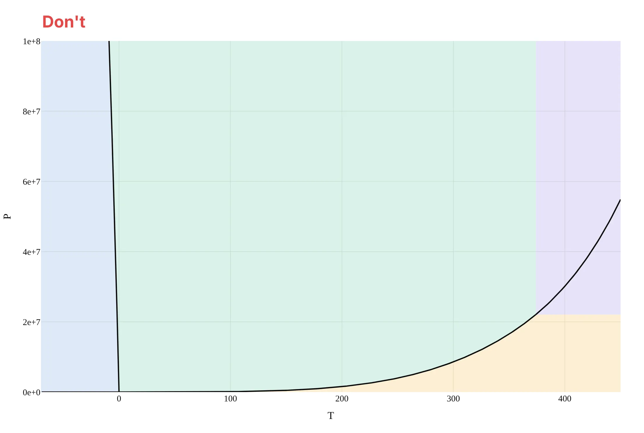
Most phase diagrams that are hard to read squeeze the interesting boundaries into one corner, or leave out the points and labels a reader needs to trust them. Here is the water diagram both ways, with the same regions and colors.
Don't use a linear pressure axis in raw pascals, which squeezes the melting, sublimation and boiling lines and the triple point into the bottom edge, carry the boiling line on past the critical point as if water still boiled there, leave the regions and the triple and critical points unlabeled, name the axes "T" and "P" without units, and keep a serif font:
Do put pressure on a log axis with units, stop the boiling line at the critical point, label the regions, mark and label the triple and critical points, and use clear axis titles:
Checklist
Do
- Put pressure on a log axis when the boundaries span decades, and label the ticks with units.
- End the liquid-gas line at the critical point, and draw the supercritical boundaries as dashed lines to show they are a convention.
- Label every region and mark the triple and critical points with their values.
- Say what the boundaries were computed from (an equation of state, a thermodynamic database or measurements) and at what pressure a binary diagram was drawn.
- For a binary diagram, label the two-phase regions, mark the eutectic with its temperature and composition, and say whether composition is in weight percent or mole fraction.
Don't
- Draw a phase diagram from a handful of remembered points by hand when a reference equation or database exists.
- Read a diagram as a guarantee for fast processes, because it describes equilibrium and a quenched or fast-cooled material can end up in a different state.
- Mix weight percent and mole fraction on one chart, or leave out the pressure of a binary diagram.
- Use the pure-water diagram for salty or impure water, whose boundaries move.
More phase diagram examples
Seven more phase diagrams, each with its source, the technique that makes it work and a prompt to rebuild it. They come from energy, pharmaceuticals, refrigeration, metallurgy and chemical engineering.
1. A carbon capture pipeline stays in one dense phase because it runs well above 7.4 MPa
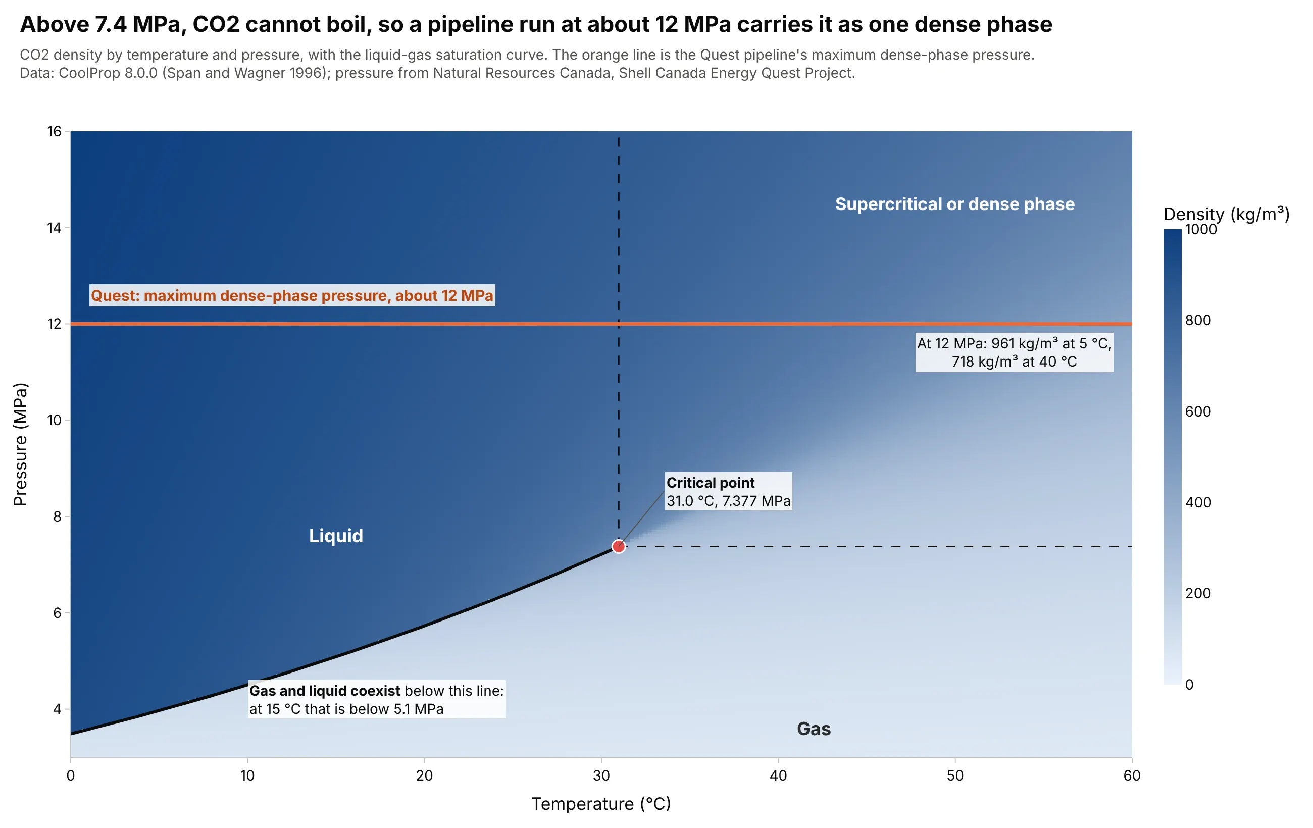
Carbon capture and storage (CCS) moves captured CO2 to an underground store, and Natural Resources Canada describes the Quest project in Alberta, which stores more than 1 million tonnes of CO2 a year about 2 km underground, as running a pipeline of up to about 12 MPa in dense phase. That is well above the 7.377 MPa critical pressure, so the CO2 cannot boil into bubbles at any temperature, and its density at 12 MPa ranges from 961 kg/m³ at 5 degrees C to 718 at 40 degrees C. Data: CoolProp 8.0.0 (Span and Wagner 1996); pressure from Natural Resources Canada, Shell Canada Energy Quest Project.
Tip: draw the saturation line heavy and end it in a marked critical point, so readers see which side of it a pipeline's pressure has to stay on.
Get the data from the CoolProp Python package (pip install CoolProp; PropsSI("D", "T", t, "P", p, "CO2") gives density inkg/m3 from the Span and Wagner equation of state) on a grid of temperature 0 to 60 C and pressure 3 to 16 MPa.Make a plotly heatmap of CO2 density with pressure in MPa on y, the saturation line from PropsSI("P", "T", t, "Q", 0, "CO2")up to the critical point (31.0 C, 7.377 MPa) drawn heavy, a horizontal line at 12 MPa, and the density at 12 MPaat 5 C and 40 C labeled.
2. Freeze-drying works below water's triple point, where ice turns straight into vapor
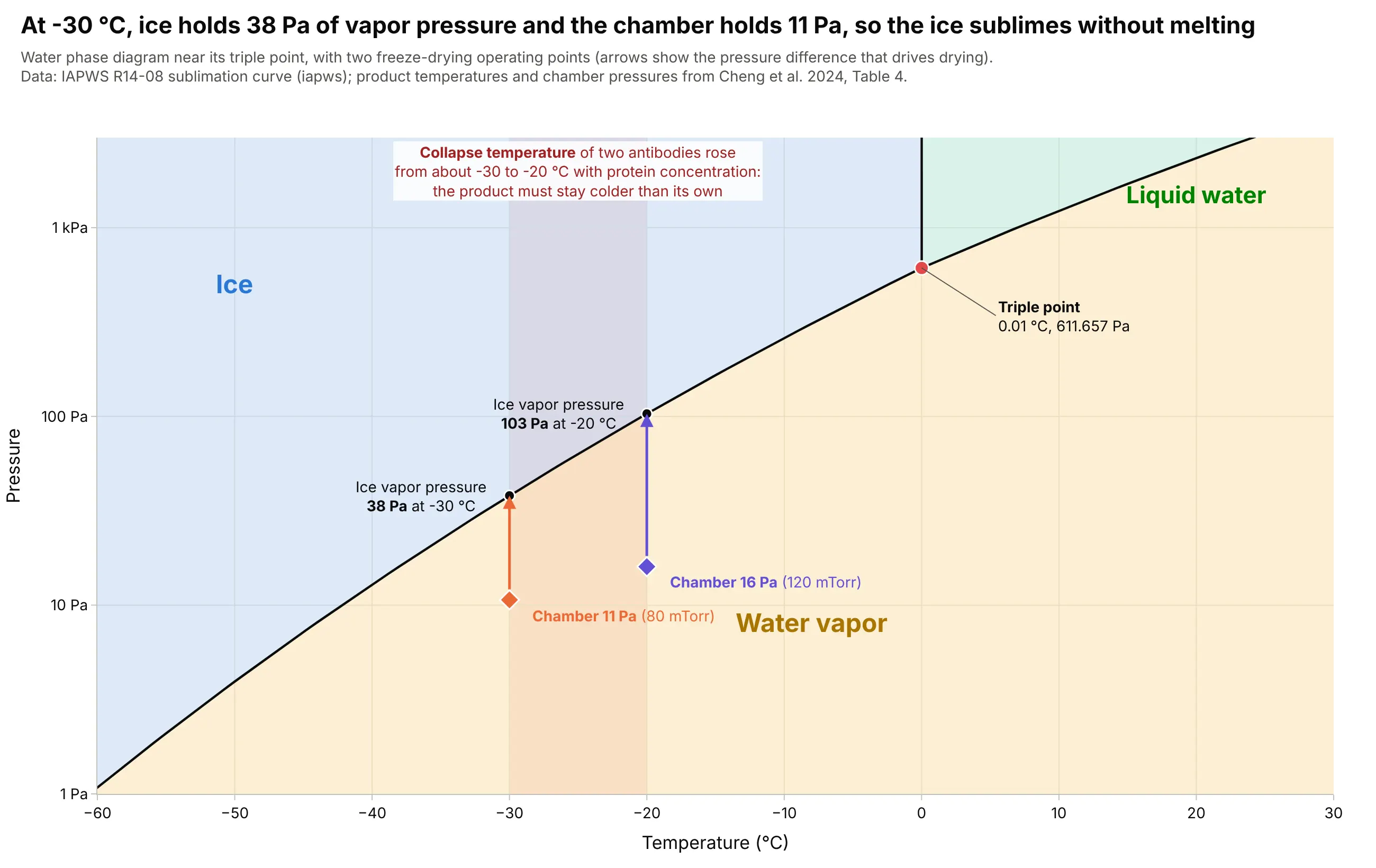
In freeze-drying, a frozen drug product sits in a vacuum chamber below water's triple point (611.657 Pa), so its ice sublimes without melting. At a product temperature of -30 degrees C, ice holds 38 Pa of vapor pressure while the chamber is held at 11 Pa (80 millitorr, mTorr), and that difference moves the water out. The product has to stay below its collapse temperature (the temperature at which the dried cake loses its structure), which a 2024 review says rose from about -30 to about -20 degrees C for two monoclonal antibodies as the protein concentration increased. Data: IAPWS sublimation curve; the operating pairs of -30 degrees C with 80 mTorr and -20 degrees C with 120 mTorr are from Cheng et al. 2024, Antibody Therapeutics 8(1):13-25, Table 4.
Tip: zoom the water diagram to the sublimation line and draw an arrow from the chamber pressure up to the ice's vapor pressure, because that gap is what drives drying.
Get the data from the iapws Python package (iapws._iapws._Sublimation_Pressure(T) in MPa and _Melting_Pressure for ice Ih,iapws.iapws97._PSat_T for the boiling line) over -60 to 30 C, and from Table 4 of Cheng et al. 2024, "Practical advice in thedevelopment of a lyophilized protein drug product" (Antibody Therapeutics 8(1)): product temperature -30 C with chamberpressure 80 mTorr, and -20 C with 120 mTorr (1 mTorr = 0.1333 Pa).Make a plotly phase diagram of water on a log pressure axis from 1 Pa to 3 kPa with light tinted regions, the triple pointmarked, and for each operating pair an arrow from the chamber pressure to the ice's vapor pressure at that temperature.Shade the band from -30 to -20 C as the collapse temperatures.
3. A methane mixture with ethane boils over a range of temperatures, and not at one
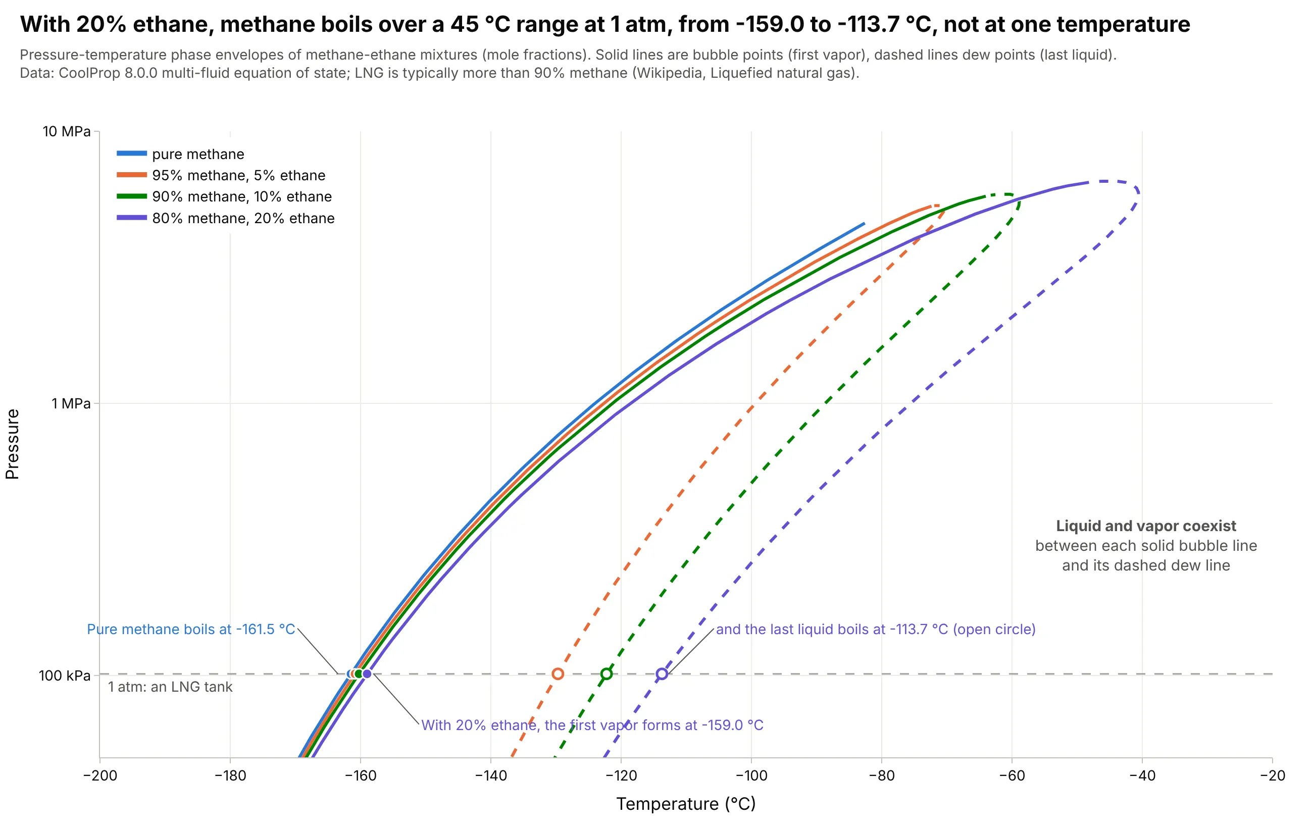
LNG is natural gas cooled to about -162 degrees C so that it is a liquid near atmospheric pressure, and it is mostly methane with some ethane. A pure substance boils on a single line, but a mixture has a bubble-point line where the first vapor appears and a dew-point line where the last liquid disappears, so with 20% ethane, methane at 1 atm starts to boil at -159.0 degrees C and finishes at -113.7, while pure methane boils at -161.5. Data: CoolProp 8.0.0 multi-fluid equation of state for the methane-ethane mixtures; LNG composition and temperature from Wikipedia.
Tip: draw the bubble line solid and the dew line dashed in the same color for each mixture, and mark the 1 atm points on both.
Get the data from the CoolProp Python package (pip install CoolProp): for the mixtures "Methane&Ethane" at methane molefractions 0.95, 0.90 and 0.80, call AbstractState("HEOS", "Methane&Ethane"), set_mole_fractions, build_phase_envelope("")and get_phase_envelope_data() for T, p and Q (Q = 1 is the dew line and Q = 0 the bubble line), and the saturation line ofpure Methane (columns: mixture, line, T_C, P_Pa).Make a plotly phase envelope chart with temperature in C on x (-200 to -20) and pressure on a log y axis from 50 kPa to10 MPa, bubble lines solid and dew lines dashed, one color per mixture, a gray dashed 1 atm line, and the bubble and dewtemperatures at 1 atm marked.
4. Carbon dioxide's critical point is below a hot day, so it runs transcritical
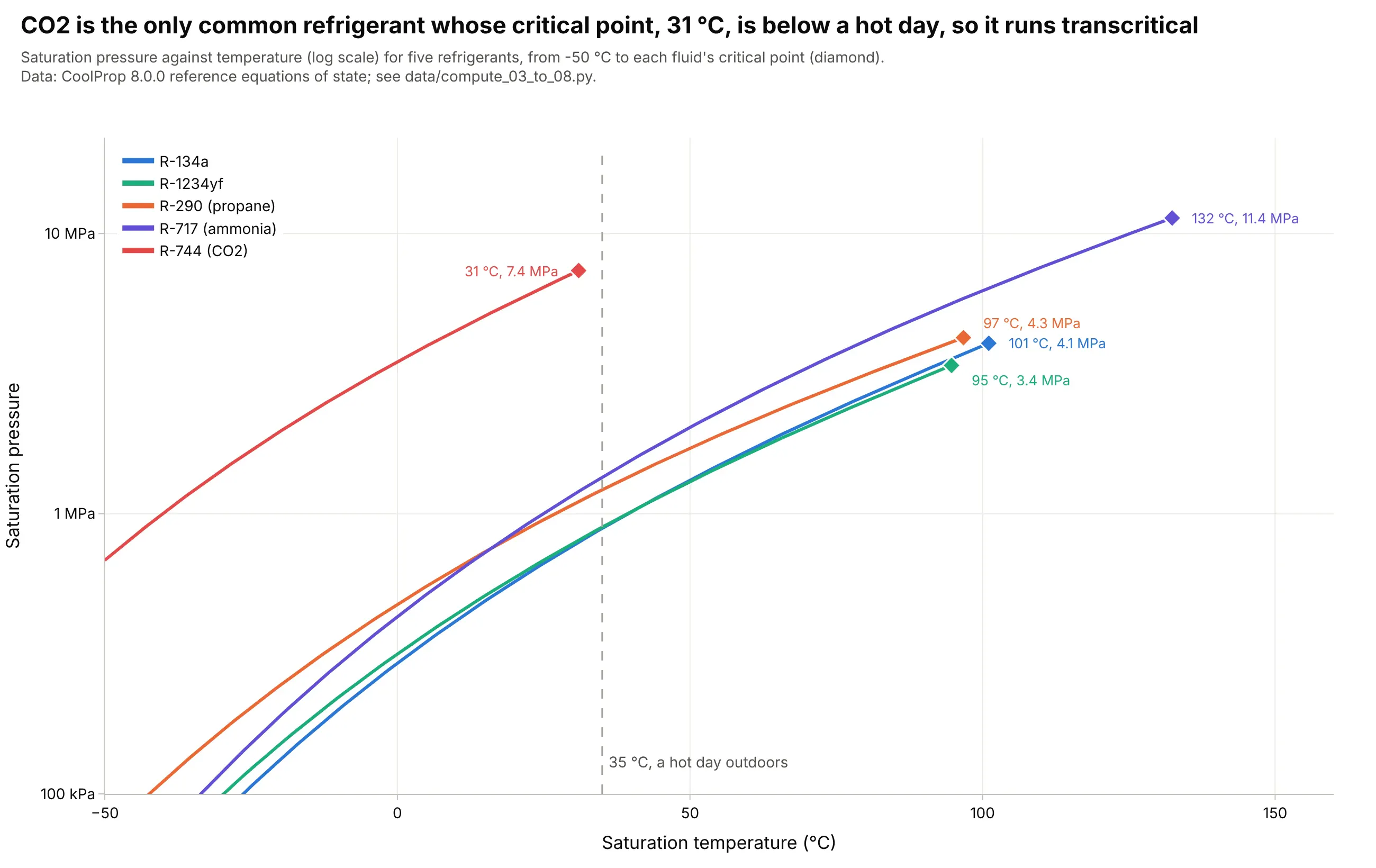
A refrigeration cycle condenses its working fluid on the saturation line, so the line has to reach the outdoor temperature. Four common refrigerants (R-134a, R-1234yf, propane and ammonia) end at critical points between 95 and 132 degrees C, but carbon dioxide (R-744) ends at 31 degrees C, so on a 35 degrees C day it cannot condense and the cycle runs transcritical, with gas cooling at a pressure above 7.4 MPa. Data: CoolProp 8.0.0 reference equations of state, from -50 degrees C to each fluid's critical point.
Tip: end each line in a marker and a label at its critical point, so the reader sees where condensing stops.
Get the data from the CoolProp Python package (pip install CoolProp; PropsSI("P", "T", t, "Q", 0, fluid) for thesaturation pressure, PropsSI("Tcrit", fluid) and PropsSI("pcrit", fluid) for the critical point) for the fluids R134a, R1234yf,Propane, Ammonia and CO2 from -50 C to their critical temperatures (columns: fluid, T_C, P_Pa).Make a plotly chart with temperature on x and pressure on a log y axis (100 kPa to 22 MPa), one line per fluid, a diamondmarker with a label (temperature, pressure) at each critical point, and a dashed vertical line at 35 C.
5. Each extra 0.1 percent of carbon in a steel adds about 14 points of pearlite
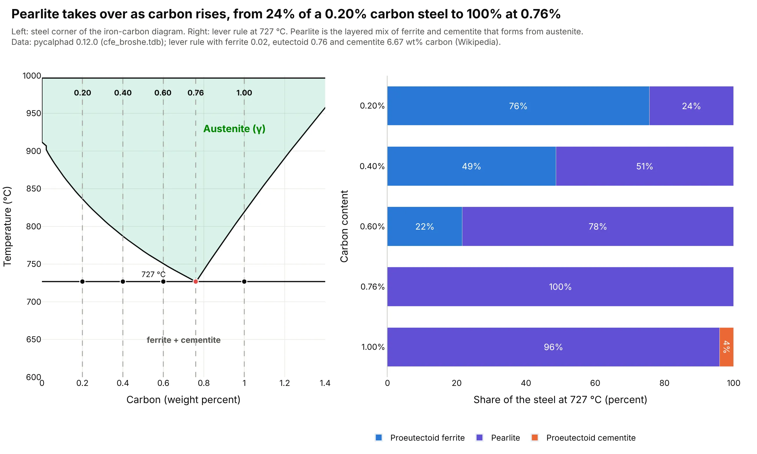
The lever rule turns the iron-carbon diagram into a microstructure. Just below 727 degrees C, a steel with 0.20 wt% carbon is 76% ferrite and 24% pearlite, one with 0.60 wt% is 22% ferrite and 78% pearlite, and one with exactly 0.76 wt% is all pearlite, so each extra 0.1 wt% of carbon in this range adds about 14 percentage points of hard pearlite. Data: diagram computed with pycalphad 0.12.0 (cfe_broshe.tdb); lever rule with the compositions given by Wikipedia, about 0.02 wt% carbon for ferrite and 6.67 wt% for cementite (Cementite) and 0.76 wt% for the eutectoid (Pearlite).
Tip: put the steels as vertical lines on the diagram next to a stacked bar of what the lever rule gives, so readers connect the line they chose with its microstructure.
Get the data from the pycalphad Python package (pip install pycalphad; Database("cfe_broshe.tdb") from pycalphad's testdatabases, phases LIQUID, BCC_A2, FCC_A1 and CEMENTITE_D011, equilibrium over carbon 0 to 25 at% and 900 to 1900 K) asweight percent carbon boundaries of the austenite field (columns: phase, T_C, wt_min, wt_max).Make a plotly figure with two panels. Left, the austenite field from 600 to 1,000 C and 0 to 1.4 wt% carbon, a line at727 C and dashed verticals at 0.20, 0.40, 0.60, 0.76 and 1.00. Right, horizontal stacked bars for those carbon contents withthe share of proeutectoid ferrite (0.76 - C) / (0.76 - 0.02), pearlite and proeutectoid cementite (C - 0.76) / (6.67 - 0.76).
6. Ethanol and water boil together near 88 mole percent ethanol, which stops distillation
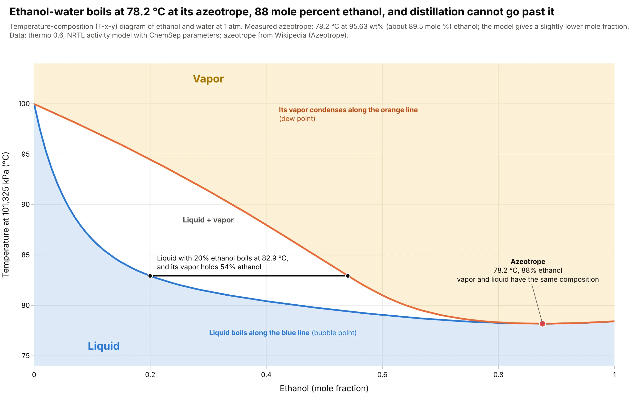
The two lines of a temperature-composition diagram show how much richer in ethanol the vapor is than the liquid it boils from, and a tie line shows it: liquid with 20 mole percent ethanol boils at 82.9 degrees C and gives vapor with 54% ethanol. The lines touch at the azeotrope, the composition where vapor and liquid are identical, so no amount of distillation goes past it. The measured value is 78.2 degrees C at 95.63 wt% ethanol (about 89.5 mole percent), and the model puts it at 87.6 mole percent. Data: thermo 0.6, a non-random two-liquid (NRTL) activity model with ChemSep parameters and Design Institute for Physical Properties (DIPPR) vapor pressures; measured azeotrope from Wikipedia.
Tip: draw a tie line at one composition, because it shows what the two curves mean faster than any caption.
Get the data from the thermo Python package (pip install thermo; ChemicalConstantsPackage.from_IDs(["ethanol", "water"]),an NRTL model from IPDB.get_ip_asymmetric_matrix("ChemSep NRTL", ...), GibbsExcessLiquid and FlashVL) as the bubble-pointand dew-point temperatures at 101325 Pa for ethanol mole fractions 0 to 1 (columns: x_ethanol, T_bubble_C, T_dew_C, y_ethanol).Make a plotly T-x-y diagram with the bubble line in blue, the dew line in orange, light tinted liquid and vapor regions, atie line at x = 0.20, and the azeotrope (the minimum of the bubble line) marked with its temperature and composition.
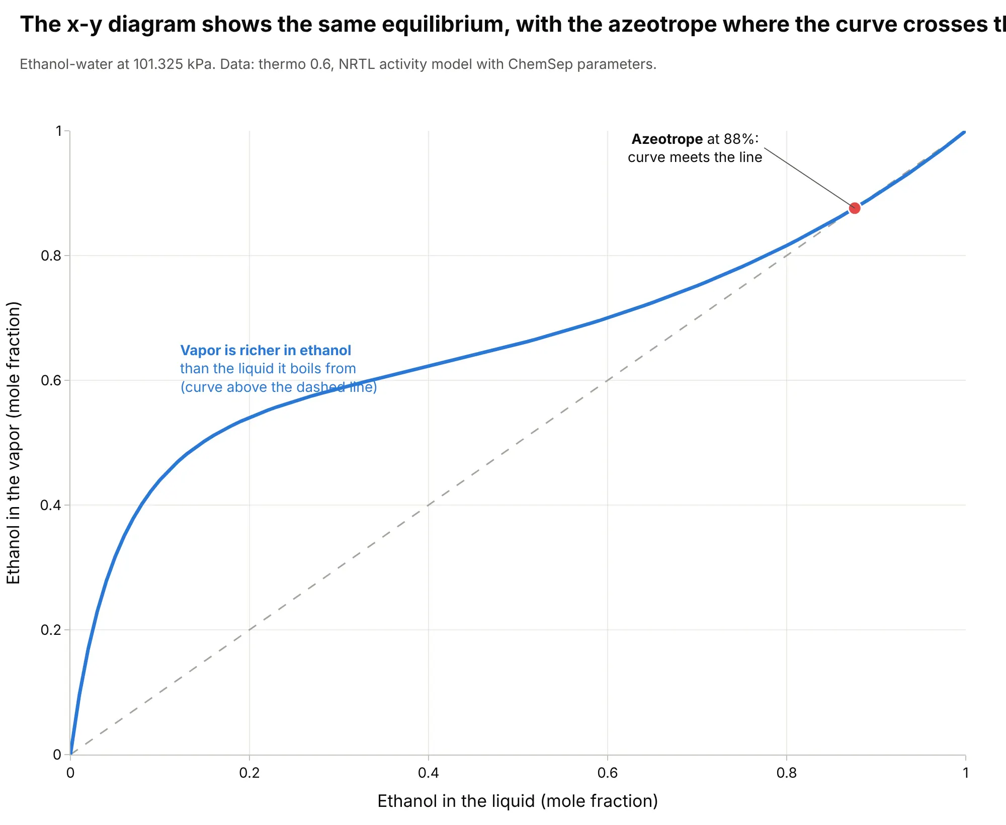
Another way to see it: chemical engineers often draw the same equilibrium as an x-y diagram, vapor composition against liquid composition, where the curve crosses the diagonal at the azeotrope.
7. Above 22.064 MPa, water never boils, which is how supercritical power plants work
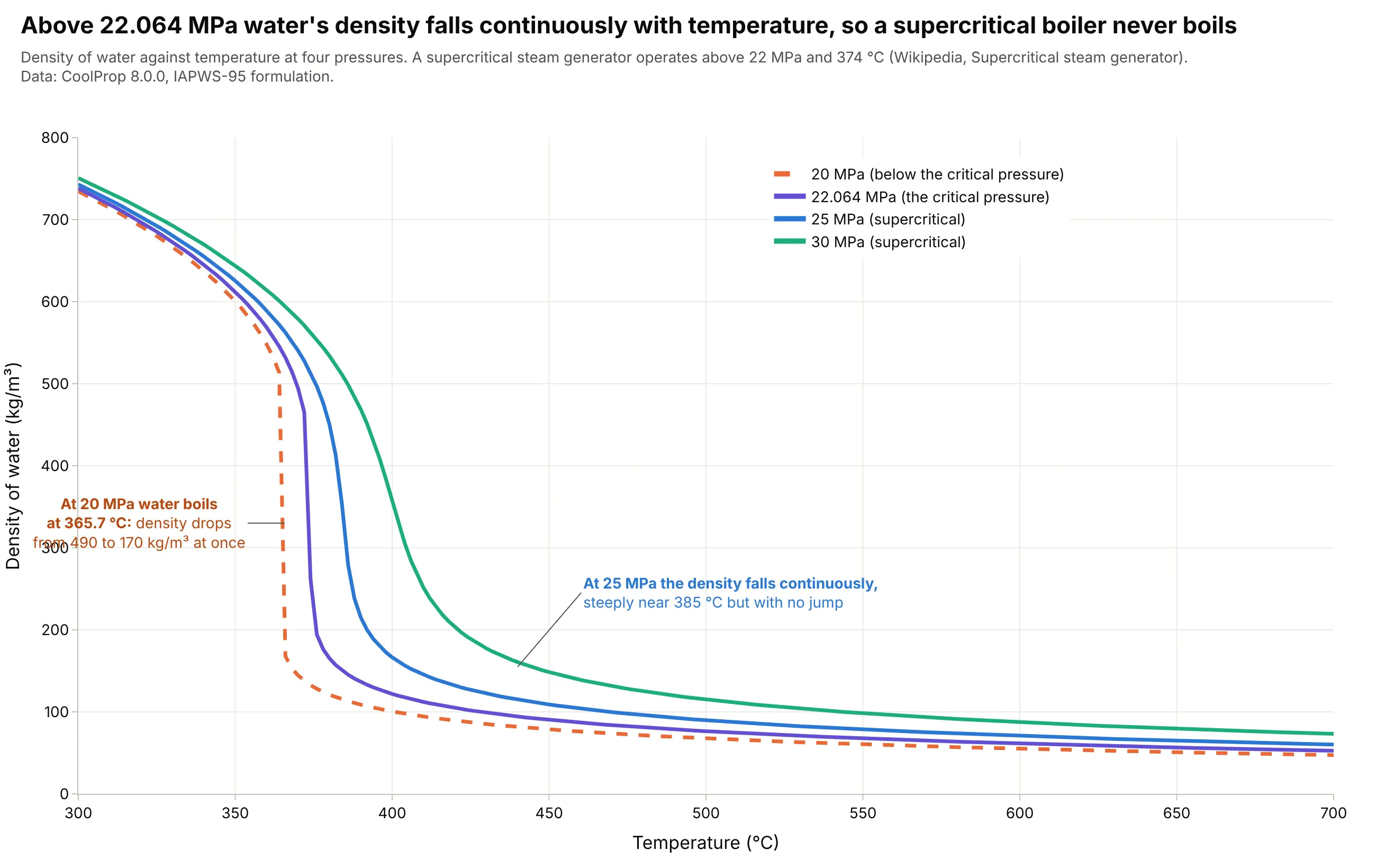
At 20 MPa, below the critical pressure, water boils at 365.7 degrees C and its density drops from 490 to 170 kg/m³ at once. At 25 MPa the density falls continuously, with its steepest drop near 385 degrees C, so a supercritical steam generator, which operates above 22 MPa and 374 degrees C, has no boiling and no separate steam and water. Data: CoolProp 8.0.0 (IAPWS-95 formulation); operating conditions from Wikipedia, Supercritical steam generator.
Tip: draw the subcritical pressure dashed and the supercritical pressures solid, so the jump stands out against the smooth curves.
Get the data from the CoolProp Python package (pip install CoolProp; PropsSI("D", "T", t, "P", p, "Water") gives density inkg/m3 from the IAPWS-95 formulation) for pressures 20, 22.064, 25 and 30 MPa over 300 to 700 C (columns: P_MPa, T_C,density_kg_m3).Make a plotly line chart with temperature on x and density on y, one line per pressure with the 20 MPa line dashed, and anannotation at the 20 MPa boiling point (365.7 C) with the density before and after.
FAQ
Options to customize
A phase diagram in Plotly is a set of lines and filled polygons, so these are the options that matter most. The full lists are in the scatter trace reference, the axes documentation and the text and annotations documentation.
- fig.update_yaxes(type="log", tickvals=[...], ticktext=[...]): a logarithmic pressure axis with tick labels that carry units (Pa, kPa, MPa).
- go.Scatter(mode="lines", hoverinfo="skip"): one trace per phase boundary, so hovering only shows your data.
- go.Scatter(fill="toself", fillcolor=...): a tinted region from a closed polygon of boundary points.
- line=dict(width=..., dash="dash"): heavy solid boundaries for phase changes and thin dashed lines for conventions such as the supercritical boundaries.
- go.Scatter(mode="markers+text") or fig.add_annotation(...): labeled triple, critical and eutectic points.
- fig.add_annotation(ax=, ay=, arrowhead=): leader lines from a label to a point, and arrows such as the pressure difference in freeze-drying (use xref="x", yref="y", axref="x", ayref="y" for data coordinates).
- fig.add_vrect(x0=, x1=) and fig.add_hline(y=): a process window, a limit temperature or the 1 atm line.
- go.Heatmap(x=, y=, z=) with colorscale: a property such as density over the whole temperature-pressure plane, under the boundaries. See the heatmap guide.
- fig.update_xaxes(type="log"): a logarithmic volume axis for pressure-volume isotherms.
- make_subplots(rows=2, cols=3): several views of the same substance, as in the alternatives figure. See the small multiples guide.